arX

iv:2

103.

0905

3v3

[m

ath.

DS]

7 J

un 2

021

Immune response in SARS-CoV-2 epidemics: A

fractional-order modelJoao P. S. Maurıcio de Carvalho1,*

1Faculty of Sciences, University of Porto, Rua do Campo Alegre s/n, Porto 4169-007, Portugal*up200902671@up.pt

ABSTRACT

Severe acute respiratory syndrome coronavirus 2 (SARS-CoV-2) is a highly contagious virus responsible for coronavirus

disease 2019 (CoViD-19). The symptoms of CoViD-19 are essentially reflected in the respiratory system, although other

organs are also affected. More than 2.4 million people have died worldwide due to this disease. Despite CoViD-19 vaccines

are already being administered, alternative treatments that address the immunopathology of the infection are still needed.

For this end, a deeper knowledge on how human immune system responds to SARS-CoV-2 is required. In this study, we

propose a non-integer order model to understand the dynamics of cytotoxic T lymphocytes in the presence of SARS-CoV-2.

We calculated the basic reproduction number and analysed the values of the model parameters in order to understand which

ones inhibit or enhance the progression of the infection. Numerical simulations were performed for different values of the

order of the fractional derivative and for different proliferation functions of cytotoxic T lymphocytes.

Introduction

In 2019, the novel coronavirus, responsible for CoViD-19, had its first outbreak in Wuhan, China1. Since then SARS-CoV-2

has reached 219 countries and territories having infected more than 100 million people, thus becoming a global pandemic and

causing more than 2.5 million deaths worldwide2–4. The main symptoms of the disease are cough, respiratory distress and

fever5. The most affected people are elderly and adults over 60 years old and/or those with comorbidities, such as obesity,

diabetes, oncological diseases, heart problems, among others6–8.

Currently, almost two years after the first outbreak, the appearance of vaccines to try to immunise the population is still

not a fast enough method to prevent the virus to spread9,10. It is becoming increasingly important to try to understand how the

immune system reacts to SARS-CoV-2 in order to find alternatives while non-priority people are not vaccinated2,11,12.

Many mathematicians have proposed several models describing the dynamics of CoViD-19 in the population13–16. How-

ever, the literature in mathematical modelling concerning SARS-CoV-2 and immune system is very limited. All the same,

there are some studies showing the dynamics of the new coronavirus in human organism, showing how healthy cells react to

the presence of the virus responsible for CoViD-19.

Literature on SARS-CoV-2 dynamics and a review of CTL proliferation functions

Wang et al.17 proposed and studied mathematical models to analyse the interaction between SARS-CoV-2, cells and immune

responses. The results of the numerical simulations allowed the authors to conclude that both anti-inflammatory treatments

and antiviral drugs combined with interferon are effective in decreasing the recovery time of individuals and in reducing the

viral plateau phase. Chatterjee et al.18 built a model to understand the dynamics of cytotoxic T lymphocytes (CTL) in the

presence of SARS-CoV-2 and in the presence of an immunostimulant drug administered at regular intervals. The authors

concluded that effective therapy can be achieved if the dosage regimen is well matched to the need of the individuals. Also,

Bairagi et al.19 proposed a model for the dynamics of an organism’s immune response to infection. The CTL response to

infection is considered to be a function of infected cells and CTL – we will call them CTL proliferation functions. The four

functions proposed and studied by the authors were:

f1(I,C) = qIC : CTL proliferation depends both on infected cells density and CTLs population;

f2(I,C) = qI : CTL production is assumed to depend on infected cells density only;

f3(I,C) =qIC

εC+ 1: CTL expansion saturates as the number of CTL grows to relatively high numbers. The level at which

CTL expansion saturates is expressed in the parameter ε;

f4(I,C) =qI

a+ εI: saturated type CTL production rate, where a is

the half-saturation constant,

and I(t) and C(t) represent the population of infected cells and CTL, respectively. In this paper, we will analyse above

functions adapted to SARS-CoV-2 infection.

Introducing fractional calculusFractional order (FO) models have been increasingly highlighted in the literature over the last few years, due to their higher

accuracy in describing non-linear phenomena20–22. The advantage of these models over models of integer order equations

consists in the number of degrees of freedom. Consequently, their comprehension covers a more extensive understanding

regarding their dynamic behaviours. In recent times, there has been a growing interest to model epidemiological systems via

non-integer order equations, and in the last two years and by virtue of circumstances, in modelling CoViD-1923–25.

Article structureFor all these reasons mentioned above, we built a FO model for the dynamics of SARS-CoV-2 in the presence of our body’s

immune response. In Section 1 we describe the proposed model and analyse some its properties about it. In Section 2 we

computed the different equilibrium states of the model and studied the basic reproduction number. In Section 3 we outline

some simulations of our dynamical system for different parameter values and for different proliferation functions. Finally, in

Section 4 we draw the conclusions about our work.

1 The model

We analyse a FO model that consists of four compartments: healthy cells susceptible to infection, T (t), infected cells, I(t),SARS-CoV-2, V (t), and cytotoxic T lymphocytes (CTL), C(t) (see Table 1). Let

Λ ={

(λ ,β ,µ ,k,δ ,N,c,q,σ ,ε,a) ∈ (R+)11}

be the set of parameters of our model. The proliferation rate of healthy cells is given by λ α . Healthy cells are infected by the

virus at a rate β α . The natural death rate of healthy and infected cells is given by µα and δ α , respectively. The term Nδ α I

represents the production of new viruses by infected cells during their lifetime. The viruses are cleared from the body at a rate

of cα . CTLs are produced through the proliferation functions fn(I,C), where f1 = qα IC, f2 = qαI, f3 = qαIC/(εC+ 1) and

f4 = qαI/(a+ εI)19. We consider qα to be the proliferation rate of CTL. The level of saturation of CTL expansion is given

by εα . Parameter aα is the half-saturation constant. The natural death rate of CTL is given by σα . Also, 0 < α ≤ 1 is the

order of the fractional derivative. The description and value of these parameters can be found in Table 3. The system of FO

equations is

dα T

dtα= λ α −β αVT − µαT

dα I

dtα= β αVT − kαIC− δ αI

dαV

dtα= Nδ α I − cαV

dαC

dtα= fn(I,C)−σαC.

(1)

We apply the principle of a FO derivative proposed by Caputo, i.e.

dα y(t)

dtα = I p−αy(p)(t), t > 0,

where p = [α] is the α-value rounded up to the nearest integer, y(p) is the p -th derivative of y(r) and I p1 is the Riemann-

Liouville operator, given by

2/13

I p1z(t) =1

Γ(p1)

∫ t

0(t − t ′)p1−1z(t ′)dt ′,

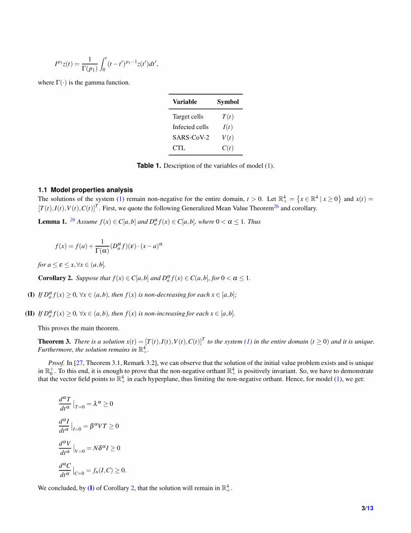
where Γ(·) is the gamma function.

Variable Symbol

Target cells T (t)

Infected cells I(t)

SARS-CoV-2 V (t)

CTL C(t)

Table 1. Description of the variables of model (1).

1.1 Model properties analysis

The solutions of the system (1) remain non-negative for the entire domain, t > 0. Let R4+ =

{

x ∈ R4 | x ≥ 0

}

and x(t) =

[T (t), I(t),V (t),C(t)]T . First, we quote the following Generalized Mean Value Theorem26 and corollary.

Lemma 1. 26 Assume f (x) ∈C[a,b] and Dαa f (x) ∈C[a,b], where 0 < α ≤ 1. Thus

f (x) = f (a)+1

Γ(α)(Dα

a f )(ε) · (x− a)α

for a ≤ ε ≤ x,∀x ∈ (a,b].

Corollary 2. Suppose that f (x) ∈C[a,b] and Dαa f (x) ∈C(a,b], for 0 < α ≤ 1.

(I) If Dαa f (x) ≥ 0, ∀x ∈ (a,b), then f (x) is non-decreasing for each x ∈ [a,b];

(II) If Dαa f (x) ≥ 0, ∀x ∈ (a,b), then f (x) is non-increasing for each x ∈ [a,b].

This proves the main theorem.

Theorem 3. There is a solution x(t) = [T (t), I(t),V (t),C(t)]T to the system (1) in the entire domain (t ≥ 0) and it is unique.

Furthermore, the solution remains in R4+.

Proof. In [27, Theorem 3.1, Remark 3.2], we can observe that the solution of the initial value problem exists and is unique

in R+0 . To this end, it is enough to prove that the non-negative orthant R4

+ is positively invariant. So, we have to demonstrate

that the vector field points to R4+ in each hyperplane, thus limiting the non-negative orthant. Hence, for model (1), we get:

dα T

dtα

∣

∣

T=0= λ α ≥ 0

dα I

dtα

∣

∣

I=0= β αV T ≥ 0

dαV

dtα

∣

∣

V=0= Nδ α I ≥ 0

dαC

dtα

∣

∣

C=0= fn(I,C)≥ 0.

We concluded, by (I) of Corollary 2, that the solution will remain in R4+.

3/13

2 Equilibria, basic reproduction number and sensitivity analysis

Throughout this section, we will be using fn(I,C) = f1(I,C) throughout this section. We will compute the following equi-

librium points of the model (1): (i) disease-free equilibria; (ii) CTL response-free equilibria; (iii) SARS-CoV-2 endemic

equilibria and study the basic reproduction number.

2.1 Disease-free equilibriaA disease-free equilibria of the model (1) is obtained via imposing I = V = C = 0. Let X0 be the disease-free equilibrium

point. Then,

X0 = (T0, I0,V0,C0) =

(

λ α

µα,0,0,0

)

.

2.2 Basic reproduction numberIn a cellular scenario, the basic reproduction number R0, is the number of secondary infections due to a single infected cell

in a susceptible healthy cell population28. Through [28, Lemma 1] the basic reproduction number can be obtained by the

following expression:

R0 = ρ(

FV−1)

, (2)

where F is the matrix of the new infection terms, V is the matrix of the remaining terms and ρ is the spectral radius of the

matrix FV−1. Thus, we get:

F =

0 β α T0

0 0

, V =

δ α 0

−Nδ α cα

.

Then, using (2) we compute R0 as:

R0 =β α T0Nδ α

(kαC0 + δ α)cα=

β αλ α

µαcαN. (3)

2.3 CTL response-free and SARS-CoV-2 endemic equilibriaThe following results show us that there is a region where a CTL response-free and SARS-CoV-2 endemic equilibria coexist.

Lemma 4. If R0 > 1, then a CTL response-free equilibria exists.

Proof. If we impose C = 0 in model (1) we get the following equilibria:

X1 = (T1, I1,V1,C1)

=

(

cα

Nβ α,

Nβ α λ α − cα µα

Nβ α δ α,

Nβ α λ α − cα µα

β αcα,0

)

.

It is clear that all cells and virus populations are non-negative. In this case it is easy to verify that T1 > 0 and C1 = 0. In order

to I1 and V1 we have (Nβ α λ α − cα µα)/(Nβ α δ α )> 0 and (Nβ α λ α − cα µα)/(β αcα)> 0, respectively. So, if

Nβ α λ α − cα µα > 0 ⇔ Nβ α λ α > cα µα (3)⇔ R0 > 1, (4)

then I1,V1 > 0. Therefore a CTL response-free equilibria exists.

We set the following real constant will be useful in the upcoming results:

ϕ0 = 1+A, (5)

where A = σα Nβ α δ α/(qαcα µα). Since A > 0, then ϕ0 > 1.

4/13

Lemma 5. If R0 > ϕ0, then a SARS-CoV-2 endemic and CTL response-free equilibria coexist.

Proof. Similar to Lemma 4, we compute the endemic equilibrium point of system (1) and we get

X2 = (T2, I2,V2,C2),

where

T2 =λ αcα qα

σα Nβ α δ α + cα µα qα

I2 =σα

qα

V2 =Nδ α σα

qα cα=

Nδ α

cαI2

C2 = B[

qα (Nβ α λ α − cα µα)−σαNβ α δ α]

,

and B = δ α/ [(σα Nβ α δ α + cα µα qα)kα ]> 0. It is clear that T2, I2,V2 > 0. Since B > 0, if

qα (Nβ α λ α − cα µα)−σαNβ α δ α > 0

⇔ qα Nβ α λ α − qαcα µα −σαNβ α δ α > 0

⇔ qα (Nβ α λ α − cα µα)> σα Nβ α δ α

⇔ Nβ α λ α − cα µα >σα Nβ α δ α

qα

⇔Nβ α λ α − cα µα

cα µα>

σα Nβ α δ α

qα cα µα

(3)⇔ R0 > 1+

σα Nβ α δ α

qαcα µα(6)

(5)⇔ R0 > ϕ0, (7)

then C2 > 0. Hence, condition (7) provides a SARS-CoV-2 endemic equilibria. Moreover, looking at expressions (4) and

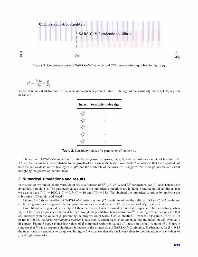
(6), we can easily verify that a CTL response-free and a SARS-CoV-2 endemic equilibria coexist. Figure 1 illustrates this

coexistence.

2.4 Sensitivity analysisSensitivity indices are a useful tool for understanding the impact that a particular parameter, p, has on the relative behaviour

of a variable, v. It is calculated through partial derivatives, using the following expression29:

γvp =

∂v

∂ p×

p

v,

where v is a differentiable function. In our case, it is important and extremely helpful to find the signs of the sensitivity indices

of R0 given in (3). In this way, we can point out which parameters contribute to the increase in viral load and which slow

down its spread. Thus, for R0, comes that

5/13

CTL response-free equilibria

SARS-CoV-2 endemic equilibria

1 ϕ00 R0

Figure 1. Coexistence space of SARS-CoV-2 endemic and CTL response-free equilibria for R0 > ϕ0.

γR0p =

∂R0

∂ p×

p

R0

.

To perform this calculation we use the value of parameters given in Table 3. The sign of the sensitivity indices of R0 is given

in Table 2.

Index Sensitivity index sign

γR0

β α +

γR0

λ α +

γR0N +

γR0

µα −

γR0

cα −

Table 2. Sensitivity indices for parameters of model (1).

The rate of SARS-CoV-2 infection, β α , the bursting size for virus growth, N, and the proliferation rate of healthy cells,

λ α , are the parameters that contribute to the growth of the virus in the body. From Table 2 we observe that the magnitude of

both the natural death rate of healthy cells, µα , and the death rate of the virus, cα , is negative. So, these parameters are useful

in fighting the growth of the viral load.

3 Numerical simulations and results

In this section we simulated the variation of R0 as a function of β α , µα , cα , N and λ α parameters (see (3)) and sketched the

dynamics of model (1). The parameter values used in the numerical simulations are in Table 3 and the initial conditions that

we assumed are T (0) = 1000, I(0) = 0, V (0) = 10 and C(0) = 333. We obtained the numerical solutions by applying the

subroutine of Diethelm and Freed32.

Figures 2 – 5 show the effect of SARS-CoV-2 infection rate, β α , death rate of healthy cells, µα , SARS-CoV-2 death rate,

cα , bursting size for virus growth, N, and proliferation rate of healthy cells, λ α , on the value of R0, for α = 1.

From literature in general, when R0 < 1 then the disease tends to slow down until it disappears. On the contrary, when

R0 > 1 the disease spreads further and further through the population being considered28. In all figures we can observe that

R0 increases with the value of β , promoting the progression of SARS-CoV-2 infection. However, in Figure 2 , for β < 0.2or for µ > 0.25, the basic reproduction number is less than 1, which leads us to conclude that the infection will eventually

disappear. Figure 3 suggests that low values of β combined with high values of c result in a small value of R0. Figure 4

suggests that N has no apparent significant influence of the progression of SARS-CoV-2 infection. Furthermore, for β < 0.15

the infection has a tendency to disappear. In Figure 5 we can see that R0 has lower values for combinations of low values of

β and high values of λ .

6/13

0.05 0.05 0.05 0.05 0.05

0.25

0.25

0.25

0.25

0.25

0.5

0.5

0.5

0.5

0.5

0.5

0.75

0.75

0.75

0.75

0.75

0.75

1

1

1

1

1

1

1.5

1.5

1.5

1.5

2

2

2

2.5

2.5

3

34

0.05 0.1 0.15 0.2 0.25 0.30

0.1

0.2

0.3

0.4

0.5

0.6

0.7

0.8

0.9

110-3

Figure 2. Effect of SARS-CoV-2 infection rate, β , and death rate of healthy cells, µ , on the basic reproduction number R0.

Initial conditions and parameter values are given in the text and in the Table 3, respectively, except for β and µ . We consider

α = 1.

0.05 0.05 0.05 0.05 0.05

0.250.25 0.25 0.25 0.25

0.5

0.50.5

0.50.5

0.75

0.75

0.750.75

0.75

1

1

1

11

1

1.5

1.5

1.5

1.5

1.51.5

2

2

2

2

2

2

2.5

2.5

2.5

2.5

2.5

3

3

3

3

3

4

4

4

1 1.2 1.4 1.6 1.8 2 2.2 2.4 2.6 2.8 30

0.1

0.2

0.3

0.4

0.5

0.6

0.7

0.8

0.9

110-3

Figure 3. Effect of SARS-CoV-2 infection rate, β and SARS-CoV-2 death rate, c, on the basic reproduction number R0.

Initial conditions and parameter values are given in the text and in the Table 3, respectively, except for β and c. We consider

α = 1.

7/13

0.05 0.05 0.05 0.05 0.05

0.25 0.25 0.25 0.25 0.25

0.5 0.5 0.5 0.5 0.5

0.75 0.75 0.75 0.75 0.75

11

1 1 1 1

1.51.5

1.51.5 1.5

22

22

22

2.52.5

2.52.5

2.5

3

3

3

33

3

4

4

4

4

4

4

10 10.5 11 11.5 12 12.5 13 13.5 14 14.50

0.1

0.2

0.3

0.4

0.5

0.6

0.7

0.8

0.9

110-3

Figure 4. Effect of SARS-CoV-2 infection rate, β , and bursting size for virus growth, N, on the basic reproduction number

R0. Initial conditions and parameter values are given in the text and in the Table 3, respectively, except for β and N. We

consider α = 1.

0.05 0.05 0.05 0.05 0.05

0.250.25 0.25 0.25 0.25

0.50.5

0.5 0.5 0.5

0.75

0.750.75

0.750.75

1

1

1

11

1

1.5

1.5

1.5

1.5

1.51.5

2

2

2

2

2

2

2.5

2.5

2.5

2.5

2.5

2.5

3

3

3

3

3

3

4

4

4

4

5 6 7 8 9 10 11 12 13 14 150

0.1

0.2

0.3

0.4

0.5

0.6

0.7

0.8

0.9

110-3

Figure 5. Effect of SARS-CoV-2 infection rate, β , and proliferation rate of healthy cells, λ , on the basic reproduction

number R0. Initial conditions and parameter values are given in the text and in the Table 3, respectively, except for β and λ .

We consider α = 1.

8/13

Parameter Symbol Value Reference

Proliferation rate of healthy cells λ α 10 cells mm−3 19

SARS-CoV-2 infection rate β α 0.001 virions mm3 day−α 30

Bursting size for virus growth N 10− 2500 virions cell−1 19

Proliferation rate of CTL qα 0.2 19

Elimination rate of infected cells by CTL kα 0.7 cells 19

Natural death rate of healthy cells µα 0.01 day−α 19

Natural death rate of infected cells δ α 1 day−α 31

Natural death rate of CTL σα 0.08 cells day−α 19

Death rate of virus cα 3 day−α 19

Level of saturation of CTL expansion ε 0.01 cells 19

Half-saturation constant a 120 cells 19

Table 3. Parameter values used in numerical simulations of model (1).

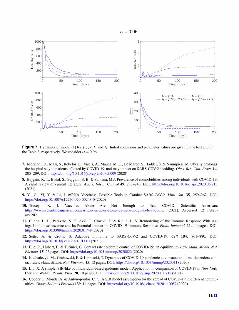
In Figures 6 – 8 we consider four different immune functions fn(I,C), specifically f1(I,C) = qαIC, f2(I,C) = qαI,

f3(I,C) = qα IC/(εC + 1) and f4(I,C) = qα I/(a+ εI), and different values of α (see figure legends). For all proliferation

functions the system presents the same asymptotic behaviour converging to an endemic state. However, it can be noted that the

number of SARS-CoV-2 infected cells and the viral load are higher when we consider the proliferation function f4. It is also

possible to notice that for the proliferation function f4, there is a higher number of infected cells. This may be a consequence

of the weak immune response (see CTL subplot). This weak immune response is also reflected in the viral load, which is also

higher for f4. The opposite is true for f1. As the immune response is stronger, the number of infected cells and the viral load

is lower. This dynamic occurs for all values of the order of the fractional derivative, α , with the particularity that the lower its

value, the less severe is the epidemic state.

4 Conclusion

In this study, a FO model for the dynamics of SARS-CoV-2, responsible for CoViD-19, was analysed together with the human

immune response, in particular CTL. The research essentially consisted of three key points:

(I): Theoretical analysis of the model to find a region where two equilibrium states can coexist.

(II): Influence that the parameters of the model have on the progression of the virus within human organism.

(III): Analysis of the immune response that human body is able to provide in the presence of SARS-CoV-2.

Regarding the coexistence of two equilibrium states, we found that under particular conditions, namely for R0 > φ0, a

CTL response-free and a SARS-CoV-2 endemic equilibria coexist (see Figure 1).

With respect to the basic reproduction number, R0, we concluded through analysis of sensitivity indices and numerical

simulations that the SARS-CoV-2 infection rate, β , has a significant impact on the decrease of healthy cells in human body.

This leads to an increase in the viral load. However, simulations have revealed that when β < 0.2, then R0 < 1, which leads

us to conclude that the infection will tend to disappear. So human body will be healthy again and free of infection.

With regard to the analysis of the immune response to infection, we simulated the model for four CTL proliferation

functions:

f1(I,C) = qα IC, f2(I,C) = qαI, f3(I,C) =qα IC

εC+ 1, f4(I,C) =

qα I

a+ εI.

We concluded that the saturated type CTL production rate, f4, is the function that most worsens the endemic state of

infection, although all CTL proliferation functions asymptotically converge towards an endemic equilibrium. Furthermore,

we verified that CTL proliferation functions that trigger stronger immune responses, such as f1 and f3, lead to fewer infected

9/13

0 50 100 150 2000

200

400

600

800

1000

0 50 100 150 2000

2

4

6

8

10

0 50 100 150 2000

500

1000

1500

= 1

0 50 100 150 2000

100

200

300

400

Figure 6. Dynamics of model (1) for f1, f2, f3 and f4. Initial conditions and parameter values are given in the text and in

the Table 3, respectively. We consider α = 1.

cells and a less pronounced viral load. All these conclusions about the immune response to SARS-CoV-2, are consistent with

the different values of the FO derivative, α . However, the lower the value of α , the lower the endemic state of the infection.

The conclusions drawn from these models are extremely important in the conception of control programs and strategic

interventions in developed and developing countries. This could help policy makers to devise strategies to reduce heavy

economical and social burden of SARS-CoV-2 infection in the world.

Considering the scarce information relating the dynamics of SARS-CoV-2 and the immune system, we were able to obtain

solid results that may contribute to the understanding of the disease and its mechanisms of action from a mathematical point

of view. We hope in the near future to present an improved version of this model, based on more biochemical information

regarding parameter values. Additionally, we plan to include the effect of vaccination at a cellular level to study how the

immune system is reinforced and what the impact is on other cells.

References

1. Hu, B., Guo, H., Zhou, P. & Shi, Z. L. Characteristics of SARS-CoV-2 and COVID-19. Nat. Rev. Microbiol. 19, 141–154,

DOI: https://doi.org/10.1038/s41579-020-00459-7 (2021)

2. Vitiello, A., Ferrara, F., Pelliccia, C., Granata, G. & La Porta, R. Cytokine storm and colchicine potential role in fighting

SARS-CoV-2 pneumonia. Ital. J. Med. 14, 88–94, DOI: https://doi.org/10.4081/itjm.2020.1284 (2020)

3. World Health Organization (WHO): https://covid19.who.int (2021). Accessed 1 March 2021

4. Worldometers: https://www.worldometers.info/coronavirus/countries-where-coronavirus-has-spread/ (2021). Accessed 1

March 2021

5. Sun, J., He, W. T., Wang, L., Lai, A., Ji, X., Zhai, X., Li, G., Suchard, M. A., Tian, J., Zhou, J., Veit, M. & Su,

S. COVID-19: Epidemiology, Evolution, and Cross-Disciplinary Perspectives. Trends Mol. Med0 26, 483–495, DOI:

https://doi.org/10.1016/j.molmed.2020.02.008 (2020)

6. Rothan, H. A. & Byrareddy, S. N. The epidemiology and pathogenesis of coronavirus disease (COVID-19) outbreak. J

Autoimmun. 109, 4 pages, DOI: https://doi.org/10.1016/j.jaut.2020.102433 (2020)

10/13

0 50 100 150 2000

200

400

600

800

1000

0 50 100 150 2000

2

4

6

0 50 100 150 2000

200

400

600

800

1000

= 0.96

0 50 100 150 2000

100

200

300

400

Figure 7. Dynamics of model (1) for f1, f2, f3 and f4. Initial conditions and parameter values are given in the text and in

the Table 3, respectively. We consider α = 0.96.

7. Moriconi, D., Masi, S., Rebelos, E., Virdis, A., Manca, M. L., De Marco, S., Taddei, S. & Nannipieri, M. Obesity prolongs

the hospital stay in patients affected by COVID-19, and may impact on SARS-COV-2 shedding. Obes. Res. Clin. Pract. 14,

205–209, DOI: https://doi.org/10.1016/j.orcp.2020.05.009 (2020)

8. Bajgain, K. T., Badal, S., Bajgain, B. B. & Santana, M.J. Prevalence of comorbidities among individuals with COVID-19:

A rapid review of current literature. Am. J. Infect. Control 49, 238–246, DOI: https://doi.org/10.1016/j.ajic.2020.06.213

(2021)

9. Yi, C., Yi, Y. & Li, J. mRNA Vaccines: Possible Tools to Combat SARS-CoV-2. Virol. Sin. 35, 259–262, DOI:

https://doi.org/10.1007/s12250-020-00243-0 (2020)

10. Tracey, K. J. Vaccines Alone Are Not Enough to Beat COVID. Scientific American.

https://www.scientificamerican.com/article/vaccines-alone-are-not-enough-to-beat-covid/ (2021). Accessed 12 Febru-

ary 2021

11. Cunha, L. L., Perazzio, S. F., Azzi, J., Cravedi, P. & Riella, L. V. Remodeling of the Immune Response With Ag-

ing: Immunosenescence and Its Potential Impact on COVID-19 Immune Response. Front. Immunol. 11, 11 pages, DOI:

https://doi.org/10.3389/fimmu.2020.01748 (2020)

12. Sette, A. & Crotty, S. Adaptive immunity to SARS-CoV-2 and COVID-19. Cell 184, 861–880, DOI:

https://doi.org/10.1016/j.cell.2021.01.007 (2021)

13. Elie, R., Hubert, E. & Turinici, G. Contact rate epidemic control of COVID-19: an equilibrium view. Math. Model. Nat.

Phenom. 15, 25 pages, DOI: https://doi.org/10.1051/mmnp/2020022 (2020)

14. Kochanczyk, M., Grabowski, F. & Lipniacki, T. Dynamics of COVID-19 pandemic at constant and time-dependent con-

tact rates. Math. Model. Nat. Phenom. 15, 12 pages, DOI: https://doi.org/10.1051/mmnp/2020011 (2020)

15. Liu, X. A simple, SIR-like but individual-based epidemic model: Application in comparison of COVID-19 in New York

City and Wuhan. Results Phys. 20, 10 pages, DOI: https://doi.org/10.1016/j.rinp.2020.103712 (2021)

16. Cooper, I., Monda, A. & Antonopoulos, C. G. A SIR model assumption for the spread of COVID-19 in different commu-

nities. Chaos, Solitons Fractals 139, 14 pages, DOI: https://doi.org/10.1016/j.chaos.2020.110057 (2020)

11/13

0 50 100 150 2000

200

400

600

800

1000

0 50 100 150 2000

1

2

3

0 50 100 150 2000

200

400

600

= 0.92

0 50 100 150 2000

100

200

300

400

Figure 8. Dynamics of model (1) for f1, f2, f3 and f4. Initial conditions and parameter values are given in the text and in

the Table 3, respectively. We consider α = 0.92.

17. Wang, S., Pan, Y., Wang, Q., Miao, H., Brown, A. N. & Rong, L. Modeling the viral dynamics of SARS-CoV-2 infection.

Math. Biosci. 328, 12 pages, DOI: https://doi.org/10.1016/j.mbs.2020.108438 (2020)

18. Chatterjee, A. N. & Al Basir, F. A Model for SARS-CoV-2 Infection with Treatment. Comput. Math. Methods Med. 2020,

11 pages, DOI: https://doi.org/10.1155/2020/1352982 (2020)

19. Bairagi, N. & Adak, D. Dynamics of cytotoxic T-lymphocytes and helper cells in human immunodeficiency virus

infection with Hill-type infection rate and sigmoidal CTL expansion. Chaos, Solitons Fractals 103, 52–67, DOI:

https://doi.org/10.1016/j.chaos.2017.05.036 (2017)

20. Muresan, C. I., Dutta, A., Dulf, E. H., Pinar, Z., Maxim, A. & Ionescu, C. M. Tuning algorithms

for fractional order internal model controllers for time delay processes. Int. J. Control 89, 579–593, DOI:

https://doi.org/10.1080/00207179.2015.1086027 (2016)

21. Sweilam, N. H., Hasan, M. M. A. & Baleanu, D. New studies for general fractional financial models of awareness and

trial advertising decisions. Chaos Solitons Fractals 104, 772–784, DOI: https://doi.org/10.1016/j.chaos.2017.09.013 (2017)

22. Valério, D., Trujillo, J. J., Rivero, M., Machado, J. A. T. & Baleanu, D. Fractional calculus: a survey of useful formulas.

Eur. Phys. J. Spec. Top. 222, 1827–1846, DOI: https://doi.org/10.1140/epjst/e2013-01967-y (2013)

23. Shah, K., Arfan, M., Mahariq, I., Ahmadian, A., Salahshour, S. & Ferrara, M. Fractal-Fractional Math-

ematical Model Addressing the Situation of Corona Virus in Pakistan. Results Phys. 19, 12 pages, DOI:

https://doi.org/10.1016/j.rinp.2020.103560 (2020)

24. Awais, M., Alshammari, F. S., Ullah, S., Khan, M. A. & Islam, S. Modeling and simulation of the novel coronavirus in

Caputo derivative. Results Phys. 19, 9 pages, DOI: https://doi.org/10.1016/j.rinp.2020.103588 (2020)

25. Aba Oud, M. A., Ali, A., Alrabaiah, H., Ullah, S., Khan, M. A. & Islam, S. A fractional order mathematical model

for COVID-19 dynamics with quarantine, isolation, and environmental viral load. Adv. Differ. Equ. 2021, 19 pages, DOI:

https://doi.org/10.1186/s13662-021-03265-4 (2021)

26. Odibat, Z. M. & Shawagfeh, N. T. Generalized Taylor’s formula. Appl. Math. Comput. 186, 286–293, DOI:

https://doi.org/10.1016/j.amc.2006.07.102 (2007)

12/13

27. Lin, W. Global existence theory and chaos control of fractional differential equations. J. Math. Anal. Appl. 332, 709–726,

DOI: https://doi.org/10.1016/j.jmaa.2006.10.040 (2007)

28. van den Driessche, P. & Watmough, J. Reproduction numbers and sub-threshold endemic equilibria for compartmental

models of disease transmission. Math. Biosci. 180, 29–48, DOI: https://doi.org/10.1016/S0025-5564(02)00108-6 (2002)

29. Chitnis, N., Hyman, J. M. & Cushing, J. M. Determining important parameters in the spread of malaria through the

sensitivity analysis of a mathematical model. Bull. Math. Biol. 70, 1272–1296, DOI: https://doi.org/10.1007/s11538-008-

9299-0 (2008)

30. Tang, S., Ma, W. & Bai, P. A Novel Dynamic Model Describing the Spread of the MERS-CoV and the Expression of

Dipeptidyl Peptidase 4. Math. Methods Med. 2017, 6 pages, DOI: https://doi.org/10.1155/2017/5285810 (2017)

31. Gonçalves, A., Bertrand, J., Ke, R., Comets, E., de Lamballerie, X., Malvy, D., Pizzorno, A., Terrier, O., Calatrava, M. R.,

Mentré, F., Smith, P., Perelson, A. S. & Guedj, J. Timing of Antiviral Treatment Initiation is Critical to Reduce SARS-CoV-2

Viral Load. DOI: https://doi.org/10.1101/2020.04.04.20047886 (2020)

32. Diethelm, K. & Freed, A. D. The FracPECE Subroutine for the Numerical Solution of Differential Equations of Fractional

Order. In: Heinzel S, Plesser T. (eds.) orschung und wissenschaftliches Rechnen: Beitrage zum Heinz-Billing-Preis 1998,

pp. 57–71. (1999)

Acknowledgements

Thanks to Beatriz Moreira-Pinto for sharing her biological knowledge, extremely important for the development of this work.

13/13