Embed Size (px)
Citation preview

UNIVERSIDADE DE SÃO PAULOINSTITUTO DE FÍSICA DE SÃO CARLOS
Vinicius Henrique Aurichio
Immersed-interface methods in the presence of shockwaves
São Carlos
2019


Vinicius Henrique Aurichio
Immersed-interface methods in the presence of shockwaves
Thesis presented to the Graduate Programin Physics at the Instituto de Física de SãoCarlos, Universidade de São Paulo, to obtainthe degree of Doctor in Science.
Concentration area: Basic Physics
Advisor: Prof. Dr. Attilio CucchieriCo-advisor: Profa. Dra. Maria Luiza Bam-bozzi de Oliveira
Original version
São Carlos2019

I AUTHORIZE THE REPRODUCTION AND DISSEMINATION OF TOTAL ORPARTIAL COPIES OF THIS DOCUMENT, BY CONVENCIONAL OR ELECTRONICMEDIA FOR STUDY OR RESEARCH PURPOSE, SINCE IT IS REFERENCED.
Aurichio, Vinicius Henrique Immersed-interface methods in the presence of shockwaves / Vinicius Henrique Aurichio; advisor AttilioCucchieri; co-advisor Maria Luísa Bambozzi de Oliveira --São Carlos 2019. 85 p.
Thesis (Doctorate - Graduate Program in Física Básica) -- Instituto de Física de São Carlos, Universidade de SãoPaulo - Brasil , 2019.
1. Immersed-interface methods. 2. Navier-Stokesequations. 3. Shock waves. I. Cucchieri, Attilio,advisor. II. de Oliveira, Maria Luísa Bambozzi, co-advisor. III. Title.

FOLHA DE APROVAÇÃO
Vinícius Henrique Auríchio
Tese apresentada ao Instituto de Física de São Carlos da Universidade de São Paulo para obtenção do título de Doutor em Ciências. Área de Concentração: Física Básica.
Aprovado(a) em: 03/05/2019
Comissão Julgadora Dr(a). Attilio Cucchieri
Instituição: (IFSC/USP)
Dr(a). Paulo Celso Greco Junior
Instituição: (EESC/USP)
Dr(a). Leonardo Paulo Maia
Instituição: (IFSC/USP)
Dr(a). Murilo Francisco Tomé
Instituição: (ICMC/USP)
Dr(a). José Antônio Silveira Gonçalves
Instituição: (UFSCar/São Carlos)


To Krissia, who always believed I could do it.And to our cats, Marie and Erwin, that were always looking.


ACKNOWLEDGEMENTS
I did not write this thesis alone and I must express my gratitute to those thatsupported me along the way. I am sure this list will be far from comprehensive and thatmy words will not give them the appropriate level of recognition, but I will try my bestjust as they did for me.
I would like to thank both of my advisors, Prof. Attilio Cucchieri and Profa. MariaLuiza Bambozzi de Oliveira for all the time they dedicated to guiding me in this PhD. Icould always just walk in their rooms to discuss any topic, related to my PhD or not, andI would be welcome. It was from those conversations that everything in this thesis wasborn. They would proofread all my texts, even when I sent them just one day before adeadline. Their comments always transformed my OK texts in excellent texts. Thank youvery much for everything.
When I first entered my room in the Physics department as a PhD candidate Iimmediatly made a new friend. Cesar Uliana and I could talk about anything and neverget bored or tired of one another. It was also through him that I met many of the friendsI made during my PhD: Renata, Paulo Eduardo, Tiago, Ágide and Carlos. They would allcome to our room after lunch to drink coffee and chat, and very often that would be thebest part of my day. Our coffee group kept growing to the point where we all could notfit in my small room and we had to find a larger one. That is how I got closer to JoséRicardo, José Teixeira and Naidel, three more in this great group of friends. The littletime we shared everyday made everything better.
From my first year as an Undergraduate student until today I have been practicingkung-fu. I have met hundreds of people during the training sessions and learned a lotabout myself through all of them. I enjoyed kung-fu so much that I became the responsibleprofessor in São Carlos, after Danilo—who was teaching me at the time—had to leave thecity to work. Once I became a professor I had the honor to teach great students. Gustavo,Natalia, Michelle, Gabriel Fabiano, Gabriel Lopes, Nicolas and Sérgio Zanchetta wouldalways learn fast and happily replace me in class, whenever I needed some extra time towrite a piece of code, or send an abstract at the last minute.
About one year ago I had to move from São Carlos and work. This was a bigchange and, at times, it seemed to me I would not be able to finish my PhD. But I ama very lucky person after all. My immediate bosses, Henrique and Ricardo, were veryunderstanding whenever I had to take a day-off to attend to academic activities and alsowhenever I arrived like a zombie at work after a sleepless night writing this thesis. Manyof my co-workers have academic degrees of their own and understood what I was going

through from experience, and all of them encouraged me to proceed. José Vitor, Thais,Giulia, Gabriel, Caio, Julia, Mariana, Verna, Wesley, Afonso, Daniela San Juan, DanielaSaito, André, Priscila, Regiane, thank you very much for your support.
Marta, Thereza, André, Paulo Matias and Joseana, you are all amazing people. Iknow you all for more than a decade now and our friendship never gets old. André andPaulo, most of what I know about computers came from being in touch with you throughthese years. Marta, Thereza and Joseana, you have seem me whole and broken, and helpedthrough every step of the way. Thank you.
Krissia, I dedicated this thesis to you and that is not nearly enough to show mygratitude towards you. You are much more than my wife. You and I know that withoutyou, even with all the support everyone else gave me, I would not have finished this thesis.We taught each other more than I thought possible and I am sure we have still to learn alot more together.
Finally, I acnkowledge CNPq for the financial support in my PhD scholarship.

“Look ma, no wiggles!.”Gino Moretti


ABSTRACT
AURICHIO, V. H. Immersed-interface methods in the presence of shockwaves. 2019. 85p. Thesis (Doctor in Science) - Instituto de Física de São Carlos,Universidade de São Paulo, São Carlos, 2019.
Fluid motion has always been of great importance for humanity since much of our progresshas been related to our understanding of fluid dynamics and to our control over the fluidssurrounding us. In particular, the experimental techniques and the methods for numericalsimulation developed during the last century allowed for great progresses both in creatingnew technologies and in improving old ones. Despite the great importance of experimentaltechniques, measuring all properties of a fluid throughout the whole domain, withoutintefering with the flow to be studied, is impossible. Also, building models even in scaleis usually expansive. Both of these reasons have driven the development of numericalmethods to the point they became an invaluable tool for fluid dynamic studies and themain tool for developing engineering solutions. If numerical methods are to be of anyuse, though, they have to correctly describe the problem geometry as well as capture therich dynamics in a variety of flow situations, such as turbulence, boundary-layers andshock-waves. This thesis addresses two of these problems. In particular, I show modifiedversions of two immersed-interface methods to describe the geometry, simplifying theirimplementations with no impact to their applicability. I also introduce two methodsfor handling shock-waves: first aiming to minimize computational costs, then improvingshock-wave resolution without increasing the number of grid points.
Keywords: Immersed-interface methods, Navier-Stokes equations, shock waves.


RESUMO
AURICHIO, V. H. Métodos de interface imersa na presença de ondas dechoque. 2019. 85p. Tese (Doutorado em Ciências) - Instituto de Física de São Carlos,Universidade de São Paulo, São Carlos, 2019.
O movimento dos fluidos sempre foi de grande importância para a humanidade, dadoque muito de nosso progresso esteve intimamente relacionado a um entendimento maisprofundo de fluidodinâmica e de como controlar os flúidos ao nosso redor. Em particular,os métodos experimentais e de simulação computacional, desenvolvidos no último século,nos permitiram grandes avanços na criação de novas tecnologias e na otimização das jáexistentes. Apesar de sua grande importância, as dificuldades de se mensurar todas aspropriedades de um flúido em todo o espaço, sem interferir com o comportamento dofluxo, além dos custos de se elaborar experimentos em tamanho real ou em escala, fez comque cada vez mais os métodos numéricos se tornassem uma importante ferramenta noestudo da fluido dinâmica e a principal ferramenta para o desenvolvimento de soluções deengenharia. Porém, para efetivamente substituir experimentos, os métodos numéricos temque ser capazes de corretamente descrever a geometria do problema, além de capturaremtodo tipo de comportamento apresentado pelos flúidos, como turbulência, camada limitee ondas de choque. Esta tese busca contribuir com dois destes desafios. Em particular,mostro versões modificadas de métodos de interface imersa para a descrição da geometria,simplificando as implementações originais sem prejudicar sua aplicabilidade. Tambémabordo métodos para tratar ondas de choque: primeiro buscando minimizar o esforçocomputacional e depois buscando aumentar a resolução do choque sem precisar refinar amalha computacional.
Palavras-chave: Métodos de interface imersa, equações de Navier-Stokes, ondas dechoque.


LIST OF FIGURES
Figure 1 – von Kármán vortices. Even though a mountain in an island (hundredsof meters) and a small cylinder (few centimeters) have different scales,the flow around the body in both systems exhibit the same vortexpattern, the so-called von Kármán vortex sheet. The occurrence of thiseffect depends mainly on the Reynolds number of the flow, one of thecharacteristic values obtained by combining the reference values of thesystem. . . . . . . . . . . . . . . . . . . . . . . . . . . . . . . . . . . . 30
Figure 2 – Examples of body-fitted meshes around a NACA0012 airfoil. Structuredmeshes are topologically equivalent to a Cartesian grid. Multiblockmeshes combine multiple structured meshes to adapt to more com-plex geometries. Finally, unstructured meshes partition the domain inarbitrarily-shaped non-overlapping pieces. . . . . . . . . . . . . . . . . 34
Figure 3 – Regular grid with ∆x spacing. Dashed lines are at the mid-point betweentwo consecutive grid points. The labels are simplified, so a point markedwith i should be interpreted as being at position xi. . . . . . . . . . . 37
Figure 4 – The function in blue has a discontinuity at a point between xi and xi+1,marked by the dashed red line. The discontinuity is at a distance η∆xfrom xi. The points at either side of the discontinuity are marked green. 39
Figure 5 – A simplified view of (fig 4). The discontinuity is shown as a red dot withtwo green dots inside and the function is omitted. This representationwill be useful later as it can be used for any type of discontinuity, suchas those originating from immersed bodies and shock waves. . . . . . . 39
Figure 6 – Two discontinuities surrounding the point xi. The first is at a distanceε∆x from xi−1. The second is at a distance η∆x from xi. . . . . . . . . 40
Figure 7 – Two discontinuities surrounding points xi and xi+1. This is similar to(fig 6) but with two regular points in between the discontinuities. . . . 40
Figure 8 – A Cartesian grid with a blue curve representing the interface between asolid region and the fluid. The blue line is the result of the interpolationof the blue points. . . . . . . . . . . . . . . . . . . . . . . . . . . . . . 43
Figure 9 – The ghost-point construction. The cyan dots are the mirror image ofthe red dots with respect to the interface. The black squares are themidpoint between the red and cyan points. The shaded regions markthe regions in which the bilinear interpolations are constructed. . . . . 44

Figure 10 – The same interface as in (fig 8), but with the crossings between theinterface and the grid lines marked in red. These points are the sametype of discontinuity represented in (fig 5), but I have omitted theinternal green dots for simplicity. . . . . . . . . . . . . . . . . . . . . . 47
Figure 11 – Different causes for shock-wave formation. In every case, flow variablesbecome discontinuous at the shock-layer. . . . . . . . . . . . . . . . . 49
Figure 12 – A shock wave separating high- and low-pressure regions. In the vicinityof the dashed rectangle we consider only the flow component normal tothe shock interface. The shock-wave velocity w is positive in the normaldirection facing the high-pressure region. In (b) we have a more detailedview of the dashed rectangle, including the sizes hy, hax, hbx of each side. 50
Figure 13 – Discretization of a step function. The discontinuity between xi−1 and ximakes it impossible for uni−1 = uni to apply, even when the grid is refined. 53
Figure 14 – Panel (a) shows a solid body (segment BC) in a high-Mach numberflow (V∞/c∞ > 1). The body abscissa b is a given fixed function. Theshock abscissa s is a function of time and y that we want to determine.A coordinate transformation f : (x, y) → (ζ, Y ) maps the physicaldomain in (a) into the computational domain in (b). . . . . . . . . . . 56
Figure 15 – Solution for the flow around a circular cylinder body obtained using theboundary shock-fitting method (the x and y coordinates are rescaled byR = ln ρ). The dots and the dashed line were obtained by Belotserkivskii1
and were used for comparison by Abbett and Moretti.2 . . . . . . . . . 56
Figure 16 – Two moving pistons generating shock-waves. The thick solid lines showthe pistons paths and the shock paths. The point in the space-timediagram where shock-waves are formed can be found analytically and aremarked as hollow circles. The dashed lines are the contact discontinuitiesand the thin solid lines are lines of constant velocity. . . . . . . . . . . 58
Figure 17 – Schematic representation of Riemann variables following the characteris-tics lines in the space-time diagram. Black solid lines represent constantR1 and gray dashed lines represent constant R2. The blue line at thebottom is the dependency domain of the blue circle. . . . . . . . . . . 59
Figure 18 – Schematic representation of R2 Riemann variable following the charac-teristics lines in the space-time diagram near a shock. The black solidline represent the shock path at the transition between a supersonicregion (to the left) and a subsonic region (to the right). . . . . . . . . 61

Figure 19 – The solid line is a plot of the function defined by (eqn 4.48). The functionis almost linear for all M > 1 values. Also, Σ > 1 if and only if M > 1.The dashed line is the function defined in (eqn 4.50) and is used as afirst guess in the iterative procedure. Here, we considered γ = 7/5 for adiatomic gas. . . . . . . . . . . . . . . . . . . . . . . . . . . . . . . . . 62
Figure 20 – Two characteristic lines carrying R2 with slopes λ(a)2 , λ
(b)2 starting at
points xi, xi+1 respectively. After a time t∗ the lines meet. If ∆t > 0.22t∗
we include a tentative shock between xi and xi+1 and keep it if it isstrong enough. . . . . . . . . . . . . . . . . . . . . . . . . . . . . . . . 63
Figure 21 – Initial conditions for the standard Sod’s shock-tube problem. On theleft side of the membrane the fluid has ρL = 1.0, uL = 0, pL = 1.0,while it has ρR = 0.125, uR = 0, pR = 0.1 on the right side. The valuesof e are a direct consequence of the others quantities. . . . . . . . . . . 65
Figure 22 – Exact results for Sod’s shock-tube problem at t = 1. Three mainstructures are evidenced in gray from left to right: an expansion fan, acontact discontinuity, and a shock-wave. . . . . . . . . . . . . . . . . . 66
Figure 23 – Results of Sod’s shock-tube problem simulated using flux-splitting tech-nique. Some dissipative effects are evident across the contact disconti-nuity and the shock wave. . . . . . . . . . . . . . . . . . . . . . . . . . 67
Figure 24 – Sod’s shock-tube problem simulated using WENO convection scheme.The numerical solution is closer to the exact solution and the disconti-nuities are resolved withing fewer mesh points in comparison to (fig 23).. . . . . . . . . . . . . . . . . . . . . . . . . . . . . . . . . . . . . . . . 67
Figure 25 – Sod’s shock-tube problem simulated using the hybrid method. Thesolution is almost identical to the one obtained using WENO method,but the use of a computationally inexpensive method in the continuousregions makes it run about four times faster then a WENO simulation. 68
Figure 26 – The three solutions discussed are compared on the same plot. The colorsare the same as in (fig 23), (fig 24) and (fig 25): flux-splitting in blue,WENO in red, and the hybrid method in green. The difference betweenthe red and green curves is minimal. . . . . . . . . . . . . . . . . . . . 69

Figure 27 – Density profile of a floating-shock reflecting from a wall (black dashedline). The initial conditions are such that ρl = 8/3, ul = 5/4, pl = 45/14to the left of the shock, and ρr = 1, ur = 0, pr = 5/7 to the right of it.From top to bottom the panels show: the system’s initial conditions,the shock approaching the wall, the system moments after the shockinteracts with the wall, the shock moving away from the wall. Boththe shock and the wall boundaries are described by the same basedata-structure and are treated identically when computing numericalderivatives. . . . . . . . . . . . . . . . . . . . . . . . . . . . . . . . . . 70
Figure 28 – Navier-Stokes simulation of a cylinder of unit diameter at Mach numberMa = 0.5, Reynolds number Re = 500, and Prandtl number Pr = 1,performed on a 400 × 200 regular Cartesian grid over the domain[0, 10]×[−2.5, 2.5]. The top and bottom domain boundaries are adiabaticno-slip walls. The left domain boundary is a subsonic inlet with aparabolic velocity profile. The right domain boundary is a subsonicoutlet. The cylinder is described using Ghias IIM and convection isperformed using a simple central-differencing scheme for all derivatives.Time evolution is obtained using the third-order accurate Runge-Kuttascheme of section 2.5.6. The accumulation of numerical errors leads toan unphysical checkerboard pattern in the density field, visible in thecenter of the figure. . . . . . . . . . . . . . . . . . . . . . . . . . . . . 71
Figure 29 – Navier-Stokes simulation of a unit diameter cylinder under the sameconditions used in (fig 28) except for the convective terms discretizationscheme. Using WENO scheme for the convective terms controls theoscillations appearing in (fig 28) resulting in a physically acceptablesolution. . . . . . . . . . . . . . . . . . . . . . . . . . . . . . . . . . . 72
Figure 30 – Navier-Stokes simulation of a unit diameter cylinder under the same con-ditions used in (fig 28) adding a filtering step. The filtering smoothes thesolution by damping the high-frequency components, thus eliminatingthe checkerboard pattern from (fig 28). . . . . . . . . . . . . . . . . . 73
Figure 31 – Navier-Stokes simulation of a unit diameter cylinder under the sameconditions considered in (fig 30) except for the immersed-interfacemethod used to describe the cylinder. Here, the simulation was performedusing Karagiozis boundary description and the results are similar butnot identical to those obtained in (fig 30), due to the difference inboundary conditions at the interface. The blue jagged pattern visiblenear the interface is an artifact of plotting and it is not related to thesimulation results. . . . . . . . . . . . . . . . . . . . . . . . . . . . . . 74
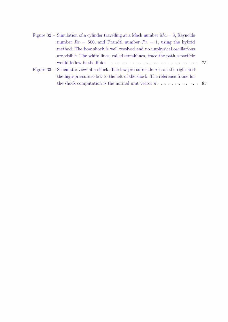
Figure 32 – Simulation of a cylinder travelling at a Mach number Ma = 3, Reynoldsnumber Re = 500, and Prandtl number Pr = 1, using the hybridmethod. The bow shock is well resolved and no unphysical oscillationsare visible. The white lines, called streaklines, trace the path a particlewould follow in the fluid. . . . . . . . . . . . . . . . . . . . . . . . . . 75
Figure 33 – Schematic view of a shock. The low-pressure side a is on the right andthe high-pressure side b to the left of the shock. The reference frame forthe shock computation is the normal unit vector n. . . . . . . . . . . . 85


LIST OF SYMBOLS
x ≡ x1 y ≡ x2 Cartesian coordinates
∆x, ∆y Grid spacing in x and y directions respectively
xi Coordinate x = xmin + i∆x
yi Coordinate y = ymin + i∆y
φi Quantity φ evaluated at position x = xi
φi,j Quantity φ evaluated at position x = xi, y = yi
φni Quantity φ evaluated at position x = xi and time t = tn
Cp Specific heat at constant pressure
Cv Specific heat at constant volume
γ = Cp/Cv Heat capacity ratio
δ = (γ − 1)/2 Convenient definition
κ Thermal condutivity
µ Viscosity
ρ Fluid density
u ≡ u1, v ≡ u2 Velocity in the x and y directions respectively
T Temperature
e = CvT Internal energy (ideal gas)
p = (γ − 1)ρe Pressure (ideal gas)
E = ρ(e+ (u2 + v2)/2) Total energy
τxx ≡ τ11, τxy ≡ τ12, τyx ≡ τ21, τyy ≡ τ22 Viscous stress tensor components
qx ≡ q1, qy ≡ q2 Heat flux in the x and y directions respectively
c =√γp/ρ Speed of sound (ideal gas)
S = 1γ(γ−1) ln (p/ργ) Entropy (ideal gas)
Re = ρwL/µ Reynolds number for some velocity w and reference length L

Pr = Cpµ/κ Prandtl number
Ma = w/c Mach number for some velocity w
δij Kronecker delta
CONTENTS
1 INTRODUCTION . . . . . . . . . . . . . . . . . . . . . . . . . . . . 25
2 NUMERICAL SIMULATIONS OF FLUIDS . . . . . . . . . . . . . . 292.1 Navier-Stokes equations . . . . . . . . . . . . . . . . . . . . . . . . . . 292.2 Discretizations . . . . . . . . . . . . . . . . . . . . . . . . . . . . . . . 322.2.1 Truncation errors . . . . . . . . . . . . . . . . . . . . . . . . . . . . . . . 322.2.2 Spatial discretization . . . . . . . . . . . . . . . . . . . . . . . . . . . . . 332.2.2.1 Finite difference (FD) methods . . . . . . . . . . . . . . . . . . . . . . . . 332.2.2.2 Finite volume (FV) methods . . . . . . . . . . . . . . . . . . . . . . . . . 332.2.2.3 Finite element (FE) methods . . . . . . . . . . . . . . . . . . . . . . . . . 332.2.3 Temporal integration . . . . . . . . . . . . . . . . . . . . . . . . . . . . . 332.2.3.1 Explicit time-integration methods . . . . . . . . . . . . . . . . . . . . . . 342.2.3.2 Implicit time-integration methods . . . . . . . . . . . . . . . . . . . . . . 342.3 Filtering . . . . . . . . . . . . . . . . . . . . . . . . . . . . . . . . . . . 352.4 Shock detectors . . . . . . . . . . . . . . . . . . . . . . . . . . . . . . . 352.5 Methods used in this thesis . . . . . . . . . . . . . . . . . . . . . . . . 352.5.1 Flux splitting . . . . . . . . . . . . . . . . . . . . . . . . . . . . . . . . . 352.5.2 Weighted essentially non-oscillatory method (WENO) . . . . . . . . . . . . 362.5.3 Finite differences . . . . . . . . . . . . . . . . . . . . . . . . . . . . . . . 382.5.3.1 Regular points . . . . . . . . . . . . . . . . . . . . . . . . . . . . . . . . 392.5.3.2 Irregular points . . . . . . . . . . . . . . . . . . . . . . . . . . . . . . . . 392.5.3.3 Upwind methods . . . . . . . . . . . . . . . . . . . . . . . . . . . . . . . 412.5.4 Filtering . . . . . . . . . . . . . . . . . . . . . . . . . . . . . . . . . . . . 412.5.5 Shock detector . . . . . . . . . . . . . . . . . . . . . . . . . . . . . . . . 412.5.6 Runge-Kutta integration . . . . . . . . . . . . . . . . . . . . . . . . . . . 42
3 IMMERSED-INTERFACE METHODS . . . . . . . . . . . . . . . . . 433.1 Boundary description . . . . . . . . . . . . . . . . . . . . . . . . . . . . 433.2 Ghias method . . . . . . . . . . . . . . . . . . . . . . . . . . . . . . . . 443.2.1 Bilinear interpolation . . . . . . . . . . . . . . . . . . . . . . . . . . . . . 453.3 Karagiozis method . . . . . . . . . . . . . . . . . . . . . . . . . . . . . 46
4 SHOCK WAVES . . . . . . . . . . . . . . . . . . . . . . . . . . . . . 494.1 Rankine-Hugoniot jump conditions . . . . . . . . . . . . . . . . . . . 494.2 Numerical methods to handle shock waves . . . . . . . . . . . . . . . 524.2.1 Conservative and non-conservative methods . . . . . . . . . . . . . . . . . 52

4.2.2 The role of shock detectors . . . . . . . . . . . . . . . . . . . . . . . . . . 544.3 Principles of shock-fitting . . . . . . . . . . . . . . . . . . . . . . . . . 544.3.1 Boundary shock-fitting . . . . . . . . . . . . . . . . . . . . . . . . . . . . 554.3.2 Floating shock-fitting . . . . . . . . . . . . . . . . . . . . . . . . . . . . . 574.4 A shock-fitting method for integrating Euler equations . . . . . . . . 574.4.1 Lambda scheme . . . . . . . . . . . . . . . . . . . . . . . . . . . . . . . . 584.4.2 Shock computations . . . . . . . . . . . . . . . . . . . . . . . . . . . . . 604.4.3 Shock detection . . . . . . . . . . . . . . . . . . . . . . . . . . . . . . . . 62
5 RESULTS . . . . . . . . . . . . . . . . . . . . . . . . . . . . . . . . . 655.1 One-dimensional simulations . . . . . . . . . . . . . . . . . . . . . . . 655.1.1 Shock-capturing . . . . . . . . . . . . . . . . . . . . . . . . . . . . . . . 665.1.2 Shock-fitting . . . . . . . . . . . . . . . . . . . . . . . . . . . . . . . . . 685.2 Two-dimensional simulations . . . . . . . . . . . . . . . . . . . . . . . 695.2.1 Immersed-interface methods . . . . . . . . . . . . . . . . . . . . . . . . . 695.2.2 High-speed flows . . . . . . . . . . . . . . . . . . . . . . . . . . . . . . . 71
6 CONCLUSIONS . . . . . . . . . . . . . . . . . . . . . . . . . . . . . 77
REFERENCES . . . . . . . . . . . . . . . . . . . . . . . . . . . . . . 79
APPENDIX 83
APPENDIX A – A WORKED SHOCK-COMPUTATION EXAMPLE 85

25
1 INTRODUCTION
Fluids are fundamental in our everyday lives: our bodies are composed of about70% water, we constantly breath air, Earth has most of its surface covered by water,and learning to manipulate water to irrigate crops enabled humans to settle and buildsocieties.3 For millennia, most of human understanding of fluids came from the necessity totransport them to specific areas, be it for agriculture, for human and cattle consumption,or for flood protection. This only changed when the Greek scientist Archimedes, in hiswork On Floating Bodies, introduced the law of buoyancy, also known as Archimedes’Principle. After him, various complex tools were created to manipulate fluids: waterpumps were studied in Alexandria around 120 BC under Ptolemies, Roman aqueductsefficiency was studied by Sextus Julius Frontinus around 90 DC, and the study of specificweights, automatic controls, plug valves by Islamic engineers led to the development ofmathematical theories of ratios and infinitesimals.
Significant progress was made on the theory of fluids when the Renaissance began.Leonardo da Vinci took rich notes while observing the movement of fluids, which foresawthe conservation of mass in one-dimensional steady flow. Galileo’s disciples BenedettoCastelli and Evangelista Torricelli applied the discoveries of their master to study themotion of rivers and canals, as well as the velocity of a water jet coming from the bottomof a vessel. These works summarized years of observation and enabled further progressin the theory of fluid motion. In 1663, a treatise by Blaise Pascal on the equilibrium ofliquids4 was published after his death, effectively elevating hydrostatics to a science. Pascaldeveloped simple proofs to the laws of the equilibrium of fluids that were amply confirmedby experiments. Also Sir Isaac Newton turned his attention to the movement of fluids. Inhis work Philosophiae Naturalis Principia Mathematica, while trying to understand whatmade fluids slow down, Newton concluded that the sheer stress, on an interface tangentto the direction of flow, is proportional to the velocity gradient. This particular form ofthe sheer stress is called Newton’s viscosity law, and fluids which obey this law are calledNewtonian fluids.
Leonhard Euler published the general form of the continuity equation and of themomentum equation in 1757.5 This allowed for a full description of the movement ofincompressible fluids. Let us recall that these equations were among the first partialdifferential equations to be written down. The last equation of fluid motion, the energyconservation equation, was derived 59 years later by Laplace and together with Euler’sequations of fluid dynamics allow to fully describe the movement of inviscid fluids.
Euler’s equations had an obvious flaw that made it of limited use for engineeringthough: it did not account for viscosity. In 1752, Jean le Rond d’Alembert showed that

26
Euler’s equations implied that immersed objects, moving at constant speed relative to thefluid, would not experience drag, in direct contradiction with experiments and experience.This is known as d’Alambert’s paradox and, until a solution was found, theoretical fluidmechanics and engineering were developed separately.
Even though Newton introduced the basic ideas of a mathematical formulationfor viscous effects, it was only in 1822 that Claude-Louis Navier introduced the correctterm in the momentum equation.6 Navier derived the dissipative term from intermolecularforces, but his derivation was valid only for incompressible fluids. In 1845, George GabrielStokes finally derived the same equation as Navier, only this time in a way valid forcompressible fluids as well. This equation, representing the momentum dynamics in aNewtonian dissipative medium, is know as the Navier-Stokes equation. When bundledwith the mass conservation equation and the energy equation (including the dissipativeeffects as well), they are collectively known as the Navier-Stokes equations. Analyticalsolutions to the full equations are available for a few cases, but a general solution is notknown.
Boundary-Layer theory is an interesting approach to study fluid dynamics ana-lytically. In this method, the flow far from an immersed-body is computed using Euler’sequations, since the viscous terms are negligible compared to the convective terms. Nearthe body, on the contrary, the flow is dominated by viscous effects and different solutionsneed to be found in this limit. Finally, a prescription for matching both solutions is used tocompute the flow in the whole domain. Analytical solutions can only take us so far, though.To study flows in complex geometries, such as those of interest in engineering, numericalsolutions had to be constructed. Various methods have been developed to generate suchsolutions and the impact they had in our world is impossible to overestimate. Numericalsolutions to the Navier-Stokes equations have been successfully used (to mention a fewapplications) to improve the aerodynamics of cars and airplanes by reducing drag andimproving lift, to ameliorate the hydrodynamics of boats and submarines, to design betterwater pumps and valves. Modified versions of the equations have also been used to studyreactive flows, plasma moving under magnetic fields—such as in fusion reactors, stars andinterstellar space—, granular media and non-Newtonian fluids.
Yet another challenge appears when dealing with high-speed flows: shock-waves canform. Pressure and density gradients can increase more and more as the fluid velocity getslarger, which can lead to discontinuities. These discontinuities then have to be appropriatelyhandled both numerically and analytically. Shock-waves are found in front of high-speedprojectiles and intercontinental ballistic missiles, and are the destructive drive of high-explosives. Then, it is no surprise that much of the research on shock-waves were sponsoredby military branches. There are also less belligerent applications to shock-waves, though.

27
Shock waves are used, for example, for kidney stones treatment7 and for some types oftendinopathy.8
In this thesis, I will describe methods that allow us to account for immersed solidbodies in a simulation, and the modifications demanded by the presence of shock waves inthe fluid flow. To this end, I will first introduce the main numerical methods used to studyfluid flows in chapter 2. Then I will address two of the many problems that arise in thenumerical study of fluids. First, in chapter 3, I will show methods capable of describingcomplex geometries, which are at the same time simple to implement, capable of handlingmoving boundaries, and parallelizable. Second, in chapter 4, I will describe the manyways shock-waves can be handled, giving special attention to the shock-fitting method. Inchapter 5 I show some numerical results obtained using the techniques introduced in theprevious chapters and I conclude the thesis in chapter 6 by summarizing my work.


29
2 NUMERICAL SIMULATIONS OF FLUIDS
Developing a numerical method for fluid simulation is difficult, as will be discussedin this chapter and in the next two. In particular, the non-linear nature of the governingequations of motion—the Navier-Stokes equations—creates a coupling between smallnumerical errors and the desired solution which, if not appropriately treated, can lead tounstable or unphysical solutions. An example of these types of effects will be shown in (fig28).
Here, I will first recall the Navier-Stokes equations and write them as two equivalentsets of differential equations. Then, I will discuss how numerical methods can be classifiedwith respect to both their spatial and temporal discretization. I will discuss also the topicof filtering, which helps to deal with numerical errors when using a central differencingscheme for spatial discretization. In section 2.4, in order to avoid differentiating acrossshock-wave discontinuities, I will introduce shock detectors. Finally, in the last part ofthis chapter, I will present the specific methods used in this thesis: central and upwindfinite-difference schemes, weighted essentially non-oscillatory method (WENO), a filtermethod and a shock-detector method.
2.1 Navier-Stokes equations
The Navier-Stokes equations describe the motion of heat-conducting viscous fluids.When studying these equations, it is useful to cast them in non-dimensional form.9 Thisis achieved by writing any dimensional variable φ as φφ∗, where φ is an adimensionalquantity, and φ∗ is a dimensional reference value. For instance, the density ρ∗ of dry air atstandard temperature and pressure (STP) conditions is 1.2754kg/m3. If we use this densityas our reference, we can obtain the adimensional density ρ for any value of the dimensionaldensity ρ as ρ = ρ/ρ∗. The reference values can then be combined into three dimensionlessconstants that are characteristic of the system being considered: the Reynolds number Re,the Prandtl number Pr and the freestream Mach number Ma∞. The Reynolds numberRe = ρ∗v∗L∗/µ∗ depends on the reference values of density ρ∗, velocity v∗, length L∗ andviscosity µ∗ and is usually interpreted as the ratio between inertial (convective) forces(ρ∗v∗) and viscous (dissipative) forces (µ∗/L∗). The Prandtl number Pr = Cpµ
∗/k dependson the heat capacity at constant pressure Cp, the viscosity µ∗ and the thermal conductivityk, and is defined as the ratio of viscous diffusion rate to the thermal diffusion rate. Thefreestream Mach number Ma∞ = v∗/c∞ is the ratio between the reference velocity v∗ andthe speed of sound c∞ computed from the reference values for temperature, density andvelocity. This adimensionalization procedure has two benefits: any bounds derived for thestability of the numerical methods will depend only on the characteristic constants, not

30
(a) Vortices near an island. (b) Vortices near a cylinder.
Figure 1 – von Kármán vortices. Even though a mountain in an island (hundreds of meters) anda small cylinder (few centimeters) have different scales, the flow around the body inboth systems exhibit the same vortex pattern, the so-called von Kármán vortex sheet.The occurrence of this effect depends mainly on the Reynolds number of the flow, oneof the characteristic values obtained by combining the reference values of the system.Source: (a) EARTH OBSERVATORY 10 (b) VAN DYKE 11.
on the actual reference values; it also becomes evident that solutions of the equations aredependent only on the characteristic constants. From the second statement it follows thatsystems with different sizes can have identical dynamics as long as their characteristicconstants are the same, as the example shown in (fig 2).
In their original version, the Navier-Stokes equations are written in terms of fluid’sdensity ρ, the velocity components ui, the total energy E, the pressure p, the heat-fluxcomponents qi and the stress-tensor components τij.6,12 In non-dimensional form, their2D version are written as9
∂ρ
∂t+ ∂
∂xj(ρuj) = 0 (2.1)
∂
∂t(ρui) + ∂
∂xj(ρuiuj + pδij − τji) = 0, i = 1, 2 (2.2)
∂E
∂t+ ∂
∂xj(ujE + ujp+ qj − uiτij) = 0, (2.3)
where the implied summation over repeated indices is used. Also, the characteristicconstants are incorporated to the definitions of τij and qi, so this form of the Navier-Stokesequations is the same for every system. The equations are in conservation form and theydescribe the mass conservation (eqn 2.1), the momentum conservation (eqn 2.2), and theenergy conservation (eqn 2.3). Note that there are more variables than equations, so wehave to combine the Navier-Stokes equations with the constitutive relations of the fluid of

31
interest, which in our case are
p = (γ − 1)ρe (2.4)
qj = − µ
(γ − 1)Ma2∞RePr
∂T
∂xj(2.5)
τij = 2µRe
Sij (2.6)
Sij = 12
(∂ui∂xj
+ ∂uj∂xi
)− 1
3∂uk∂xk
δij, (2.7)
where δij is the Kronecker delta. From the above equations we see that this fluid is anideal gas (eqn 2.4), obeys the Fourier law for heat transfer by conduction (eqn 2.5), isNewtonian (eqn 2.6), and has negligible bulk viscosity, which yields a viscous strain tensorwith a simple form (eqn 2.7).
It is useful to define the vectors
U =
ρ
ρu
ρv
E
(2.8)
F =
ρu
ρu2 + p
ρuv
(E + p)u
(2.9) G =
ρv
ρuv
ρv2 + p
(E + p) v
(2.10)
FD =
0τxx
τxy
τxxu+ τxyv − qx
(2.11) GD =
0τyx
τyy
τyxu+ τyyv − qy
(2.12)
so that (eqn 2.1), (eqn 2.2), and (eqn 2.3) can be summarized as
∂U
∂t+ ∂F
∂x+ ∂G
∂y= ∂FD
∂x+ ∂GD
∂y. (2.13)
The vectors F and G are called the fluid’s x and y fluxes respectively, while FD and GD
contain the dissipative terms.
When studying shock-waves in chapter 4 it will be convenient to use an alternativeform of the Navier-Stokes equations. This form can be obtained from the first one by aseries of variable changes. Instead of using the density ρ, the velocities u and v, and thetotal energy E, this form uses the sound speed c, the velocities u and v, and the entropy

32
S. Then, using δ = (γ − 1)/2, the Navier-Stokes equation become13
1δ
∂c
∂t+ 1δui∂c
∂xi− c∂S
∂t− cui
∂S
∂xi= 2δc
γp
(∂qi∂xi
+ ∂
∂xi(ujτij)
)(2.14)
∂ui∂t
+ uj∂ui∂xj
+ c
δ
(∂c
∂x1+ ∂c
∂x2
)− c2
(∂S
∂x1+ ∂S
∂x2
)= 1ρ
∂τij∂xj
, i = 1, 2 (2.15)
∂S
∂t+ ui
∂S
∂xi= 1γp
(∂qi∂xi
+ ∂
∂xi(ujτij)
). (2.16)
2.2 Discretizations
To obtain numerical solutions for the Navier-Stokes equations, presented in the lastsection, there are various possible approaches. For the purpose of this thesis it will sufficeto consider Eulerian methods—in which we describe the fluid properties in fixed points inspace—capable of simulating compressible high-speed flows. This means I will not describeLagrangian methods (e.g. Smoothed Particle Hydrodynamics14)—where the fluid particlesare tracked individually and no grid is necessary—, nor the Lattice Boltzmann method15
(suited for low Mach number, incompressible flows), nor spectral methods16 (not suitedfor flows with discontinuities such as shock waves).
2.2.1 Truncation errors
An important concept when studying numerical approximations is the truncationerror. A numerical solution obtained by any method will almost always differ from the exactsolution to the problem, and so it is necessary to measure how large is the error introducedby the approximations. Besides the absolute value of the error, different discretizationmethods have different convergence ratios with respect to refining the discretization. Tomake these ideas more concrete, let f(x) be an infinitely differentiable function, andD(f, xi) = F (fi−k, . . . , fi+m), k,m ∈ N an approximation for the first derivative, definedon a regular grid, with spacing ∆x, and evaluated at x = xi. The difference between thereal derivative and the proposed approximation is given by
df
dx
∣∣∣∣∣x=xi−D(f, xi) = TE(D) =
+∞∑m=l
αmdm+1f
dxm+1 (∆x)m, (2.17)
with αm ∈ R, l ∈ N. As shown above, the truncation error TE(D) of the approximationgiven by D can be written as a power series of the grid width ∆x. Notice that, as the gridis refined, ∆x goes to zero and so the approximation converges to the real value of thederivative. Moreover, the error term is dominated by (∆x)l, the first term in the seriesexpansion, and this determines the convergence rate of this particular approximation.It is then said that the discretization D has a truncation error of order (∆x)l, or, in ashorthand notation, that TE(D) = O
((∆x)l
). As a consequence, the discretization D
itself is said to have order l.

33
2.2.2 Spatial discretization
For the purpose of this thesis I only consider three categories of spatial discretization:finite difference, finite volume, and finite element methods.
2.2.2.1 Finite difference (FD) methods
Finite difference methods, as the name implies, approximate the spatial derivativesby differences. The points used in the discretization must form a grid, regular or not, asin (fig 2a). The accuracy of the approximation is related to the number of points used toreconstruct the derivatives. All methods employed in this thesis belong to this categoryand a more detailed description will be given in section 2.5.3.
2.2.2.2 Finite volume (FV) methods
In finite volume methods, the space is partitioned in arbitrarily shaped, non-overlapping pieces called cells. Although it is possible to combine cells of different shapes,it is usual to consider one specific shape (triangles or quadrilaterals are the most commonchoices in 2D). This allows for much more flexible meshes as shown in (fig 2b) and (fig 2c).Instead of directly computing the derivatives as in the finite difference methods, we usethe divergence theorem to pose the question differently: the rate of change of a quantitywithin a cell equals the net flux across its boundaries, so if we compute the fluxes atthe boundaries we can obtain the variation in the flow variables. The accuracy of a FVdiscretization is related to the reconstruction of the fluxes at the cells interfaces.
2.2.2.3 Finite element (FE) methods
The same meshes used in FV methods can be used to perform computations usingthe finite element methods. Here, the pieces covering the space are called elements insteadof cells. The flow-variable values are computed at some points in the element (the nodes),which allows their values at all points inside each element to be computed by interpolation.The compatibility relations between neighboring elements is given by the Navier-Stokesequations, resulting in a set of algebraic equations that must be solved at each time step.The accuracy in a FE discretization is related to the number of nodes in each element,which in turn determines the degree of the interpolating function used, as well as to thesize of each element.
2.2.3 Temporal integration
Once the space is discretized using one of the previous schemes, it is necessary tochoose a method to compute the time evolution of the Navier-Stokes equations. At anytime t of the computation the values of all flow variables φ(t) will be known and we wouldlike to determine their values at t+ ∆t, i.e. φ(t+ ∆t). There are two families of methods

34
(a) Structured mesh. (b) Multiblock mesh. (c) Unstructured mesh.
Figure 2 – Examples of body-fitted meshes around a NACA0012 airfoil. Structured meshes aretopologically equivalent to a Cartesian grid. Multiblock meshes combine multiplestructured meshes to adapt to more complex geometries. Finally, unstructured meshespartition the domain in arbitrarily-shaped non-overlapping pieces.Source: (a) JAVADI 17, (b) MANISHA 18, (c) CHEN 19
that we cover next. To this end, consider the differential equationdφ
dt= F(φ(t), t), (2.18)
where F is an arbitrary function depending on φ and t.
2.2.3.1 Explicit time-integration methods
In an explicit time-integration methods, the values of φ(t+ ∆t) depend only on thevalues of φ at previous times.20 Therefore, given φ(t) (and possibly φ(t−∆t), φ(t− 2∆t)etc), the values of φ(t+ ∆t) are immediately computable. The simplest explicit method isdue to Euler, usually called Euler method. If we apply it to (eqn 2.18) we obtain
φ(t+ ∆t)− φ(t)∆t = F(φ(t), t) (2.19)
φ(t+ ∆t) = φ(t) + ∆t F(φ(t), t). (2.20)
Notice that (eqn 2.20) explicitly gives us the value of φ(t+ ∆t).
2.2.3.2 Implicit time-integration methods
Implicit time-integration methods require the solution of an equation to obtainφ(t+ ∆t).20 This equation is sometimes linear, and it is then solvable using exact methods,such as Gaussian elimination, but it can also be non-linear and some approximation mightbe needed. The simplest implicit method is also due to Euler, the so-called backward Eulermethod, which when applied to (eqn 2.18) results in
φ(t+ ∆t)− φ(t)∆t = F(φ(t+ ∆t), t+ ∆t) (2.21)
φ(t+ ∆t) = φ(t) + ∆t F(φ(t+ ∆t), t+ ∆t). (2.22)
Note that, in contrast to explicit methods, it is not possible, in general, to obtain anexplicit expression for φ(t+ ∆t) from (eqn 2.22).

35
2.3 Filtering
Finite-difference schemes with central stencils (central-difference schemes) areinteresting because, as a consequence of their symmetry, there are no even derivativesin the truncation error, and so they have no numerical dissipation. This, however, leadsto instabilities,21 as there are no mechanism to control the growth of numerical errors.The errors can accumulate and the numerical solution becomes unphysical. A possiblesolution to this issue is to introduce filtering, a mechanism through which the highestfrequencies are attenuated. It is important to realize that the appeal of a central-differencescheme is precisely its zero-dissipation nature and that filtering introduces an artificialmechanism that is similar to dissipation to control the numerical errors. This means thatthe filtering mechanism must be chosen carefully, otherwise there will be no advantage inusing a central-difference scheme.
2.4 Shock detectors
Under certain circumstances the flow variables may develop discontinuities—suchas gradient discontinuities, contact discontinuities, and shock-waves—due to the transitionfrom subsonic to supersonic flow. It is important to detect the formation of these disconti-nuities early in the simulation in order to avoid taking numerical derivatives across them.Indeed, not only the numerical result would be unphysical, as the information can onlytravel one-way across shock-waves, but also oscillations would form, as a consequence ofthe Gibbs phenomenon. 22–24 Shock detectors are methods that can detect sharp variationsin the function, so that in regions with sharp variations an appropriate method can thenbe used.
2.5 Methods used in this thesis
After this short overview of numerical discretizations, I will detail the numericalapproximations used in this thesis. All the spatial discretizations are in the finite-differencecategory, and the time discretization used is a member of the Runge-Kutta family ofmethods.
2.5.1 Flux splitting
Two of the methods that follow depend on a separation of the flux F (G) into twocomponents, representing waves travelling along the positive and negative directions of

36
the x(y)-axis. Steger and Warming25 described a method to compute one such separationfor an ideal gas. Defining the general flux F as
F [λ1, λ3, λ4; k1, k2] = ρ
2γ
2(γ − 1)λ1 + λ3 + λ4
2(γ − 1)λ1u+ λ3(u+ ck1) + λ4(u− ck1)
2(γ − 1)λ1v + λ3(v + ck2) + λ4(v − ck2)
(γ − 1)λ1(u2 + v2) + λ32 [(u+ ck1)2 + (v + ck2)2]
+λ42 [(u− ck1)2 + (v − ck2)2] + (3−γ)(λ3+λ4)
2(γ−1)
, (2.23)
where
λ1 = k1u+ k2v (2.24)
λ3 = λ1 + c (2.25)
λ4 = λ1 − c, (2.26)
and considering
λ±1 = λ1 ± |λ1|2 (2.27)
λ±3 = λ3 ± |λ3|2 (2.28)
λ±4 = λ4 ± |λ4|2 , (2.29)
then we can write
F+ = F[λ+
1 , λ+3 , λ
+4 ; k1 = 1, k2 = 0
](2.30)
F− = F[λ−1 , λ
−3 , λ
−4 ; k1 = 1, k2 = 0
](2.31)
G+ = F[λ+
1 , λ+3 , λ
+4 ; k1 = 0, k2 = 1
](2.32)
G− = F[λ−1 , λ
−3 , λ
−4 ; k1 = 0, k2 = 1
]. (2.33)
One can verify that F = F+ + F− and G = G+ +G−, where F and G are the xand y fluxes defined in (eqn 2.9) and (eqn 2.10).
2.5.2 Weighted essentially non-oscillatory method (WENO)
Introduced by Liu, Shu and Osher26 the weighted essentially non-oscillatory method(WENO) is a popular method to compute numerical solutions of the Navier-Stokesequations, since it is capable of yielding high-order of accuracy, of handling shock-wavesand it is not very difficult to implement.

37
i i+1 i+2i-1i-2 i+3
i+1/2i-1/2i-3/2 i+3/2 i+5/2
Figure 3 – Regular grid with ∆x spacing. Dashed lines are at the mid-point between two con-secutive grid points. The labels are simplified, so a point marked with i should beinterpreted as being at position xi.Source: By the author.
I will illustrate the WENO procedure by considering the x derivative of onecomponent φ of the F+ flux. The first step is to define the following expression
∂φ
∂x
∣∣∣∣∣x=xi+1/2
= Φi+1/2 − Φi−1/2
∆x , (2.34)
which is exact as long as a suitable expression for Φ is determined. We then proceedto construct three approximations for Φi+1/2, obtained by interpolating values of Φ atdifferent grid points:
Φ(1)i+1/2 = 1
3φi−2 −76φi−1 + 11
6 φi (2.35)
Φ(2)i+1/2 = −1
6φi−1 + 56φi + 1
3φi+1 (2.36)
Φ(3)i+1/2 = 1
3φi + 56φi+1 −
16φi+2. (2.37)
Notice that the above approximations are not symmetrical with respect to the pointxi+1/2, but show a bias towards the left. This is because F+ corresponds to right-runningwaves, and so the left region is the origin of these waves. These interpolations are obtainedusing second degree polynomials and have third order accuracy. It is possible to combinethe three of them and obtain a fifth order interpolation, and this is what the essentiallynon-oscillatory method (ENO) does. The WENO method adds an extra step so thatinterpolations are only made using regions where the flow is continuous, avoiding thedegradation of the accuracy. To achieve this it is necessary to compute three smoothnessindicators for the region considered, i.e.
β1 = 1312 (φi−2 − 2φi−1 + φi)2 + 1
4 (φi−2 − 4φi−1 + 3φi)2 (2.38)
β2 = 1312 (φi−1 − 2φi + φi+1)2 + 1
4 (φi−1 − φi−1)2 (2.39)
β3 = 1312 (φi − 2φi+1 + φi+2)2 + 1
4 (φi+2 − 4φi+1 + 3φi)2 . (2.40)
The next step will create ponderators that will make a particular approximationmore important than the others if it is in a smoother region. These ponderators (afterthe next step) are identical to those obtained in the ENO method if the three regions are

38
equally smooth. The ponderators σ are
σ1 = 110
1(β1 + ε)2 (2.41)
σ2 = 35
1(β2 + ε)2 (2.42)
σ3 = 310
1(β3 + ε)2 , (2.43)
where ε is a small number (e.g. 10−30) to avoid a division by zero. Also, the sigmas arenormalized to create the final ponderators ω
ω1 = σ1
σ1 + σ2 + σ3(2.44)
ω2 = σ2
σ1 + σ2 + σ3(2.45)
ω3 = σ3
σ1 + σ2 + σ3. (2.46)
Finally the approximated value of Φi+1/2 can be obtained as
Φi+1/2 = ω1Φ(1)i+1/2 + ω2Φ(2)
i+1/2 + ω3Φ(3)i+1/2. (2.47)
This procedure is repeated with the adequate shift to obtain Φi−1/2 and (eqn 2.34) is thenused to obtain ∂φ/∂x.
A similar calculation can be employed to compute all four components of thederivative of the flux vector F+. We must also compute the derivative of F− followingessentially the same procedure. It suffices to note that if we reverse the x-axis, the F−
waves are now running in the same direction of the reversed axis, so we can repeat exactlythe same procedure. Of course, as there is no essential difference between the x and y axis,it is trivial that the same procedure applies also to G±.
2.5.3 Finite differences
Sometimes the WENO method described above is not necessary or it is not practical.Simple problems do not need its adaptative behaviour, and it might be too slow for theapplication, because of the number of operations necessary to compute it. Finite differencesmethods are reasonable alternatives in these cases. I will consider two categories of points:regular and irregular. Points in the fluid bulk are in the former category, and points nearinterfaces are in the latter one.

39
Figure 4 – The function in blue has a discontinuity at a point between xi and xi+1, marked bythe dashed red line. The discontinuity is at a distance η∆x from xi. The points ateither side of the discontinuity are marked green.Source: By the author.
Figure 5 – A simplified view of (fig 4). The discontinuity is shown as a red dot with two greendots inside and the function is omitted. This representation will be useful later as itcan be used for any type of discontinuity, such as those originating from immersedbodies and shock waves.Source: By the author.
2.5.3.1 Regular points
For a flow variable φ, the second-order accurate first and second derivatives arecalculated as
∂φ
∂x
∣∣∣∣∣x=xi
= 12∆x (φi+1 − φi−1) +O((∆x)2) (2.48)
∂2φ
∂x2
∣∣∣∣∣x=xi
= 1(∆x)2 (φi+1 − 2φi + φi−1) +O((∆x)2), (2.49)
in the case of a regular point at x = xi.
2.5.3.2 Irregular points
If the expressions in (eqn 2.48) and (eqn 2.49) are applied to the function in figure(fig 4) at xi+1 the result is non-zero in both cases, but clearly the function is constant tothe right of the discontinuity, and the analytical result is zero for both derivatives. Also,the O((∆x)2) truncation error derived for the expressions above is only valid where thefunction being derived is smooth. Indeed, the actual error when taking a derivative acrossa discontinuity is O(1). It is then necessary to derive special expressions to compute thederivatives near discontinuities.

40
Figure 6 – Two discontinuities surrounding the point xi. The first is at a distance ε∆x from xi−1.The second is at a distance η∆x from xi.Source: By the author.
Denoting the value to the left of the discontinuity as φld and the value to the rightas φrd, a first-order expression for the first derivative, at a point with a discontinuity to it’sleft, e.g. xi+1 in (fig 4), or to it’s right, is given by
∂φ
∂x
∣∣∣∣∣l
x=xi= 1
(1 + (1− η))∆x (φi+1 − φrd) +O(∆x) (2.50)
∂φ
∂x
∣∣∣∣∣r
x=xi= 1
(1 + η)∆x(φld − φi−1
)+O(∆x). (2.51)
The expression for a second derivative with a discontinuity to it’s left is
∂2φ
∂x
∣∣∣∣∣l
x=xi= 2
(2− η)(3− η)(∆x)2 (φrd − (3− η)φi+1 + (2− η)φi+2) +O(∆x). (2.52)
Another possibility is that two discontinuities surround the point where the deriva-tive is being computed as in (fig 6). The expression obtained for the first derivative is then
∂φ
∂x
∣∣∣∣∣x=xi
= 1((1− ε) + η)∆x
(φldη − φ
rdε
)+O(∆x), (2.53)
where φrdε is the value to the right of the discontinuity to the left of xi, and φrdη is thevalue to the left of the discontinuity to the right of xi. For stability reasons this derivativeis only computed if (1− ε) + η > 1, otherwise it is set to zero. The second derivative isalways set to zero in this configuration.
Figure 7 – Two discontinuities surrounding points xi and xi+1. This is similar to (fig 6) but withtwo regular points in between the discontinuities.Source: By the author.
A final case to consider is shown in (fig 7). The first derivatives are computed using(eqn 2.50) and (eqn 2.51), but the second derivative must be computed using
∂2φ
∂x
∣∣∣∣∣x=xi
= 4((2 + η − ε) ∆x)2
(φrdε − 2
(η + ε
2 (φi+1 − φi))
+ φdη
). (2.54)

41
2.5.3.3 Upwind methods
We can explore further25 the flux-splitting method introduced in section 2.5.1.Let’s consider only the flux component F+ for a moment. As mentioned, the flux F+
represent waves travelling from left-to-right along the x-axis. We can incorporate thisphysical interpretation into the numerical method by computing one-sided (or biased)derivatives of F+, favoring the direction where the waves are coming from. This can beinterpreted as a mean to enforce the correct dependency domain at a given point. Onlythe region from where the waves are coming (i.e. upwind from the point) will influence it.Of course the same arguments are equally applicable to the F− component. The simplestapproximation for the convective term derived from this idea is
∂F
∂x
∣∣∣∣∣x=xi
= F+i − F+
i−1∆x + F−i+1 − F−i
∆x . (2.55)
2.5.4 Filtering
As mentioned in section 2.3, when applying FD methods based on central-differences,the numerical errors accumulate due to the lack of numerical dissipation, and high-frequencyunphysical oscillations are generated. This effect is enhanced when the Reynolds numberis high, as the system’s dissipation is low. However, if a filtering operation is applied to thegrid before each timestep, this unphysical oscillations can be controlled and a reasonablenumerical solution can be obtained. Here, I chose to apply the filter introduced by Vasilyev27 to control the oscillations. In this case, a filtered flow variable φ is computed as
φi = − 116φi−1 + 1
4φi−1 + 58φi + 1
4φi+1 −116φi+2 (2.56)
φi = + 116φi−1 + 3
4φi + 38φi+1 −
14φi+2 + 1
16φi+3 (2.57)
φi = +1516φi + 1
4φi+1 −38φi+2 + 1
4φi+3 −116φi+4, (2.58)
where (eqn 2.56) is to be used in the fluid bulk, and (eqn 2.57) and (eqn 2.58) nearthe domain boundaries. No special treatment is necessary near discontinuities due toshock-waves.
2.5.5 Shock detector
Two different methods were used to detect shocks. In this chapter I will onlydescribe one of them, leaving the other to chapter 4. In 2016, Bambozzi and Pires 28
introduced a shock-detector capable of detecting discontinuities not only in the function,but in any of it’s derivatives. The shock detector works by comparing the approximationobtained using all the grid points with the approximation obtained using, say, only theodd grid points. If the function is sufficiently smooth, both approximations will be verysimilar, but if there is a discontinuity they will be different. Let F (n)
∆x denote the n− th

42
derivative of function F approximated using all grid points, and F (n)2∆x the same derivative
approximated using only the odd numbered grid points. The shock detector∗ comparesthese approximations by computing
Sd = log2
(2∆x)2∣∣∣F (2)
2∆x
∣∣∣+ (2∆x)3∣∣∣F (3)
2∆x
∣∣∣(∆x)2
∣∣∣F (2)∆x
∣∣∣+ (∆x)3∣∣∣F (3)
∆x
∣∣∣ . (2.59)
The value of Sd is enough to infer the function continuity since
Sd ≈
2, if F is continuous up to it’s 1st derivative
p, if F has a jump in it’s p < 2 derivative.(2.60)
2.5.6 Runge-Kutta integration
Runge-Kutta methods are a family of iterative methods, used to compute ap-proximate solutions for the time-evolution of systems described by ordinary differentialequations. This family includes both explicit and implicit methods. In particular, the Eulermethod and the backward Euler method of section 2.2.3 are examples of Runge-Kuttamethods. The system time evolution in every simulation in this thesis is computed usingthe following third-order explicit method
∂φ
∂t= F(φ(t), t) (2.61)
k1 = F(φ(t), t) (2.62)
k2 = F(φ(t) + ∆t2 k1, t+ ∆t
2 ) (2.63)
k3 = F(φ(t)−∆tk1 + 2∆tk2, t+ ∆t) (2.64)
φ(t+ ∆t) = φ(t) + ∆t6 (k1 + 4k2 + k3) . (2.65)
Here F is a generic function. In particular, if we identify φ with U from (eqn 2.8) and use
F(φ(t), t) = −∂F∂x− ∂G
∂y+ ∂FD
∂x+ ∂GD
∂y(2.66)
we can time-evolve the Navier-Stokes equations.
∗ This is not the shock-detector version used in28, but the same results apply to this one.

43
3 IMMERSED-INTERFACE METHODS
In 1952, Hyman 29 introduced a method to solve elliptic equations using an arbitraryinterface embedded in the domain with a Cartesian grid-based discretization. This methodwas further developed and is now well established in the works of Leveque30, Li31,32 andZhong.33 These fictitious domain methods present two advantages: first, numerical solverscan be made very efficient by leveraging the regularity from the underlying Cartesiangrid and second, introducing new arbitrary interfaces is inexpensive in comparison withremeshing.
In 1971, Charles Peskin was studying the blood flow in the heart. He developed anumerical method 34 to simulate the presence of a moving, flexible immersed boundary toaccount for the presence of a leaflet in a heart valve. Peskin’s method was the first workto apply the ideas from Hyman’s work to fluid dynamical problems, creating a class ofmethods known as immersed-boundary methods (IBM). In this method, the boundarymovement is coupled to the fluid movement using a distributed force that spreads theboundary influence to neighbouring points, making the interface diffuse. Other methods,such as those used by Ghias35 and Karagiozis,36compute the effects of the interface atits exact position keeping the interface sharp. I will describe how these last two methodswork in this chapter.
3.1 Boundary description
Consider the solid-fluid interface in (fig 8). The interface is described as series ofmarker points, shown as blue dots in the figure, that are later interpolated. In this thesis,
Fluid
Solid
Figure 8 – A Cartesian grid with a blue curve representing the interface between a solid regionand the fluid. The blue line is the result of the interpolation of the blue points.Source: By the author.

44
Fluid
Solid
Figure 9 – The ghost-point construction. The cyan dots are the mirror image of the red dotswith respect to the interface. The black squares are the midpoint between the red andcyan points. The shaded regions mark the regions in which the bilinear interpolationsare constructed.Source: By the author.
I have used cubic splines to obtain the blue curve. See ref.37 for a detailed explanation onhow splines are computed.
Both Karagiozis and Ghias methods are identical up to this point. I will nowdescribe how each proceed from this point.
3.2 Ghias method
Ghias employs a ghost-point based method to account for immersed interfaces. Theeffect of the boundary is substituted by flow-variable values, attributed to some pointsinside the immersed bodies (the ghost points).
Before further discussing the advantages and disadvantages of this method, let’ssee in detail how the ghost-points values are obtained. Using (fig 9) as a reference:
• For each point inside the body with at least one neighbour in the fluid (the ghostpoints, marked as red circles) compute the point on the boundary that is closest toit (the boundary intercepts, marked as black squares);
• Compute the mirror image of the ghost point with respect to the boundary intercept(the image points, marked as cyan circles);
• For each image point, determine the four grid points closest to it. If one of suchpoints is a ghost point, replace it for it’s corresponding boundary intercept. Theshaded quadrilateral regions are formed connecting the four points obtained for eachimage point in the figure;

45
• Compute the flow variables at the image points using a bilinear interpolation (detailedin section 3.2.1) constructed using the four points obtained in the last step;
• Use the values at the image points and their corresponding boundary intercepts toextrapolate the ghost-point values.
The method I have described has an important difference when compared to theoriginal paper.35 I substitute the ghost points for their boundary intercept at the thirdstep. Ghias only makes this substitution when the neighbouring ghost point is the onecorresponding to the image point, such as in the leftmost shaded region. He later uses aniterative method to solve the coupled equations. I find the method I employed easier toimplement and it also produces good results.
This procedure keeps the computational grid regular everywhere making the useof irregular derivatives unnecessary, and makes it easy to use powerful methods—suchas the WENO method—in combination with it. On the downside, however, computingsuitable values for the ghost points needs a bilinear interpolation and an extrapolation,and there is also a significant increase in the overall computational geometry complexity.The computational geometry steps required to determine both the image points and theinterpolation weights also makes the handling moving boundaries more involved.
Now that we know how to compute the flow variables at the ghost points, we cantime-evolve the system. For each Runge-Kutta substep:
• Compute the flow variables at the grid points;
• Compute the fluxes at all grid points using derivatives for regular points;
• Time-evolve the solution using the computed fluxes.
Notice that it is not necessary to recompute the fluxes this time.
3.2.1 Bilinear interpolation
As mentioned at the end of chapter 2 I will describe the bilinear interpolation35
used to compute the flow variables values at the image points. We consider a function ofthe form
Φ(x, y) = a+ bx+ cy + dxy, (3.1)
where the values of a, b, c, d are obtained from the four image-point neighbours. Rememberthat some of the neighbours might be boundary-intercept points, and that at these pointsa Neumann boundary condition can be enforced. When that is the case, we do not havedirect access to the function value at the neighbour point, but only to it’s normal derivativeat that point.

46
I will first describe how to obtain the coefficients when the function values areknown at all four points. This situation arises when either all four neighbours of the imagepoint are fluid points, or the boundary conditions being enforced are Dirichlet boundaryconditions.To this end, write
1 x1 y1 x1y1
1 x2 y2 x2y2
1 x3 y3 x3y3
1 x4 y4 x4y4
a
b
c
d
=
Φ1
Φ2
Φ3
Φ4
, (3.2)
where xi, yi are the coordinates x and y of the image-point neighbours and Φi is thefunction value at that point. Once solved, (eqn 3.2) yields the four coefficients a, b, c, dand it is possible to compute Φ(x, y) at the image point. If the boundary is static, thecoordinates xi, yi are fixed and the square matrix on the left hand side of (eqn 3.2) canbe inverted once at the start of the computation and stored to be reused.
Let’s now consider the case of Neumann boundary conditions. Suppose withoutloss of generality that the fourth neighbour of an image point is a boundary-interceptpoint and that the boundary condition
~n · ~∇Φ = Ψ (3.3)
is to be enforced. Careful manipulation of the equations will lead to the new system ofequations
1 x1 y1 x1y1
1 x2 y2 x2y2
1 x3 y3 x3y3
0 nx ny nxy4 + nyx4
a
b
c
d
=
Φ1
Φ2
Φ3
Ψ
(3.4)
where nx, ny are the components of the outward-normal unit vector at the boundary point.Once again, if the boundary is static the matrix can be inverted once at the beginning ofthe computation and stored to be reused.
3.3 Karagiozis method
Instead of constructing auxiliary points as in Ghias method, Karagiozis utilizes theboundary explicitly in his method. Karagiozis method begins marking the points wherethe interpolated interface crosses the grid lines as shown in (fig 10). Then, it enforcesDirichlet or Neumann boundary conditions on the flow variables at these points, and thatis how the immersed interface is accounted for in the simulation.
Dirichlet boundary conditions are used to enforce the no-slip condition for viscousflows, and to fix the body temperature. Remember from (fig 5) that each discontinuity hasan internal structure, so enforcing Dirichlet boundary conditions is as simple as setting

47
Fluid
Solid
Figure 10 – The same interface as in (fig 8), but with the crossings between the interface and thegrid lines marked in red. These points are the same type of discontinuity representedin (fig 5), but I have omitted the internal green dots for simplicity.Source: By the author.
the internal values appropriately. Density values at the boundary are obtained using alinear extrapolation from the neighboring points.
Consider the discontinuity in (fig 5). To compute the density ρ to the left (ρld) ofand to the right (ρrd) of the discontinuity we use
ρld = ρi + (ρi − ρi−1) η (3.5)
ρrd = ρi+1 + (ρi+1 − ρi+2) (1− η). (3.6)
Now that we have a procedure to enforce the boundary conditions we can computethe time evolution of the system. For each Runge-Kutta substep:
• Enforce all boundary conditions;
• Compute the fluxes at all grid points using derivatives for regular points;
• Recompute the fluxes at points near immersed interfaces using derivatives for irregularpoints;
• Time-evolve the solution using the computed fluxes.
In this chapter I showed two methods to describe solid bodies embedded in fluidusing immersed-interfaces that are suitable for numerical simulations of fluids. In the nextchapter I will introduce another type of discontinuity: shock waves.

49
4 SHOCK WAVES
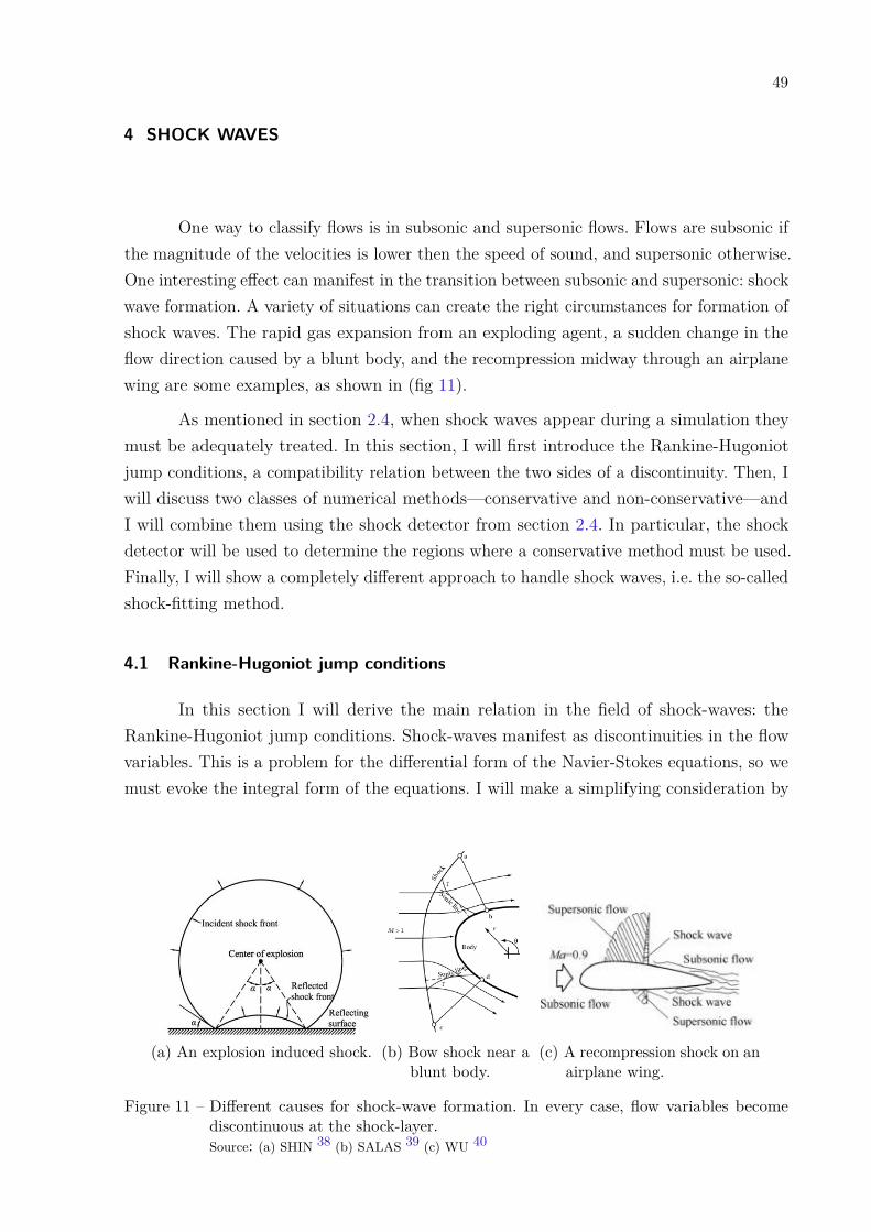
One way to classify flows is in subsonic and supersonic flows. Flows are subsonic ifthe magnitude of the velocities is lower then the speed of sound, and supersonic otherwise.One interesting effect can manifest in the transition between subsonic and supersonic: shockwave formation. A variety of situations can create the right circumstances for formation ofshock waves. The rapid gas expansion from an exploding agent, a sudden change in theflow direction caused by a blunt body, and the recompression midway through an airplanewing are some examples, as shown in (fig 11).
As mentioned in section 2.4, when shock waves appear during a simulation theymust be adequately treated. In this section, I will first introduce the Rankine-Hugoniotjump conditions, a compatibility relation between the two sides of a discontinuity. Then, Iwill discuss two classes of numerical methods—conservative and non-conservative—andI will combine them using the shock detector from section 2.4. In particular, the shockdetector will be used to determine the regions where a conservative method must be used.Finally, I will show a completely different approach to handle shock waves, i.e. the so-calledshock-fitting method.
4.1 Rankine-Hugoniot jump conditions
In this section I will derive the main relation in the field of shock-waves: theRankine-Hugoniot jump conditions. Shock-waves manifest as discontinuities in the flowvariables. This is a problem for the differential form of the Navier-Stokes equations, so wemust evoke the integral form of the equations. I will make a simplifying consideration by
(a) An explosion induced shock. (b) Bow shock near ablunt body.
(c) A recompression shock on anairplane wing.
Figure 11 – Different causes for shock-wave formation. In every case, flow variables becomediscontinuous at the shock-layer.Source: (a) SHIN 38 (b) SALAS 39 (c) WU 40

50
(a) Schematic shock wave (b) Detailed view
Figure 12 – A shock wave separating high- and low-pressure regions. In the vicinity of the dashedrectangle we consider only the flow component normal to the shock interface. Theshock-wave velocity w is positive in the normal direction facing the high-pressureregion. In (b) we have a more detailed view of the dashed rectangle, including thesizes hy, hax, hbx of each side.Source: By the author.
ignoring the dissipative terms at the position of the shock. This is justified, considering thatshock-waves are found in flows with a high Reynolds number and therefore the influenceof the dissipative terms is relatively small. From now on in this chapter I will take thedissipative terms qi and τij to be zero.
Notice that all components of the Navier-Stokes equations can be written as
∂φ
∂t+ ∂f
∂x+ ∂g
∂y= ∂φ
∂t+ ~∇ · ~H = 0 (4.1)
where φ, f and g are the components of the vectors in (eqn 2.8), (eqn 2.9) and (eqn 2.10)respectively, and ~H = fx+ gy. Consider the region marked by the dashed rectangle in(fig 12) to be infinitesimal and that the only discontinuity in the flow is due to the shockwave. Using a coordinate system with the x axis normal to the shock interface, near thedashed rectangle, we write the integral form of the equation as
d
dt
∫∫rectangle
φ dx dy = −∫∫
rectangle
~∇ · ~H dx dy (4.2)
= −[(fb − fa)hy +
((gta − gba
)hax +
(gtb − gbb
)hbx)]
+O(h2),
where I employed the divergence theorem to go from the first to the second line andh, in the error term, stands for anyone of the lengths. Also, the lengths hax and hbx arethe rectangle’s width to either side of the shock, and hy it the rectangle’s height. Thesubscripts a and b in the flux components f and g indicate if they are computed in the low-or high-pressure region, respectively. Also, the superscripts t and b in g indicate if the flux

51
is computed on the top or bottom side of the rectangle respectively. We now manipulatethe left hand side of (eqn 4.2). If we keep the outer limits of the rectangle fixed, i.e hy andhax + hbx are constant, but allow for the shock-wave to move we can write
d
dt
∫∫rectangle
φ dx dy = d
dt
[(φah
axhy + φbh
bxhy
)+O
(h3)]
(4.3)
=(dφadt
hax + φadhaxdt
+dφbdthbx + φb
dhbxdt
+O (h))hy.
Also, notice thatdhaxdt
= −dhbx
dt= w. (4.4)
Combining 4.2, 4.3 and 4.4, we obtain
w (φa − φb) + dφadt
hax + dφbdthbx = (fa − fb)−
gta − gbahy
hax −gtb − gbbhy
hbx +O(h)
= (fa − fb)−dgady
hax −dgbdyhbx +O(h), (4.5)
where we took the limit hy → 0 and used the continuity of g to identify the terms on theright hand side as derivatives. Taking the limit as hax and hbx go to zero, we finally obtain
w (φa − φb) = fa − fb. (4.6)
This is known as the Rankine-Hugoniot jump condition of a conservation law. Replacingthe specific values of φ and f found in Euler equations, we obtain
w (ρa − ρb) = ρaua − ρbub (4.7)
w (ρaua − ρbub) =(ρau
2a + pa
)−(ρbu
2b + pb
)(4.8)
w (ρava − ρbvb) = ρauava − ρbubvb (4.9)
w (Ea − Eb) = (Ea + pa)ua −(E2b + pb
)ub. (4.10)
By multiplying 4.7 by vb and subtracting 4.9 from it, we find
wρa (vb − va) = ρaua (vb − va) (4.11)
va = vb, (4.12)
where we have to impose the condition 4.12 in order to make (eqn 4.11) valid in general. Thecombination of (eqn 4.7), (eqn 4.8), (eqn 4.10) and (eqn 4.12) are the Rankine-Hugoniotjump conditions for Euler equations. They are the fundamental relations in the shock-wavetheory and will be the basis of the shock-fitting method described in section 4.3

52
Had we used the alternative form of the Navier-Stokes presented in 2.14, 2.15 and2.16, we would have obtained the equivalent jump conditions53
cb = ca
√(γM2 − δ) (1 + δM2)
(1 + δ)M (4.13)
ub = ua + ca1−M2
(1 + δ)M (4.14)
Sb = Sa + 12δγ
[ln γM
2 − δ1 + δ
− γ ln (1 + δ)M2
1 + δM2
](4.15)
vb = va (4.16)
M = ua − wca
, (4.17)
where M is the relative shock Mach number.
4.2 Numerical methods to handle shock waves
4.2.1 Conservative and non-conservative methods
Terminology can be confusing when using this classification. The components ofthe Navier-Stokes equations are conservation laws, so what is meant by a non-conservativemethod? Conservative methods are derived from the equations put in divergence form,while non-conservative methods are derived from the equations after the chain rule hasbeen applied to expand the derivatives into more terms. The methods derived from thedivergence form automatically guarantees the conservation of fluxes through a particularcontrol volume, and are thus called conservative methods. On the contrary, this is notexactly guaranteed when the method is derived from the expanded equations, and that iswhy they are called non-conservative methods.
To compare conservative and non-conservative methods I will consider the 1-DBurgers equation, which is a limiting case of the Navier-Stokes equations, i.e.
∂u
∂t+ u
∂u
∂x= 0 (4.18)
∂u
∂t+ 1
2∂u2
∂x= 0. (4.19)
Analytically, (eqn 4.18) and (eqn 4.19) are equivalent. However, (eqn 4.18) is in non-conservative form, and (eqn 4.19) is in conservative form. Moreover, consider the followingupwind discretizations (for u ≥ 0)
un+1i − uni
∆t + uniuni − uni−1
∆x = 0 (4.20)
un+1i − uni
∆t + 12
(uni )2 −(uni−1
)2
∆x = 0. (4.21)

53
Figure 13 – Discretization of a step function. The discontinuity between xi−1 and xi makes itimpossible for uni−1 = uni to apply, even when the grid is refined.Source: By the author.
It is clear that it is impossible to reduce one equation to the other. Let’s now manipulatethe second term on the left-hand side of (eqn 4.21):
12
(uni )2 −(uni−1
)2
∆x = 12
(uni + uni−1
) (uni − uni−1
)∆x
= ¯uni+ 1
2
uni − uni−1∆x (4.22)
¯uni+ 1
2= uni + uni−1
2 . (4.23)
Thus, the term obtained in (eqn 4.21) equals to the second term in (eqn 4.20) if and onlyif uni = uni−1. Let us note that, for a continuous function,
uni−1 = uni −∆x ∂u∂x
∣∣∣∣∣x=xi
+O((∆x)2
). (4.24)
Therefore, even though (eqn 4.20) and (eqn 4.21) are inequivalent, they will convergeto the same solution in the limit ∆x → 0 if u is continuous. On the other hand, if u isdiscontinuous this argument is no longer valid. Indeed, looking at the simple example in(fig 13) it is clear that, even taking the continuum limit, uni−1 and uni will never be equal.Analytically, the derivative in (eqn 4.24) becomes ill-defined at the discontinuity in thelimit ∆x→ 0, so it is not possible to justify the equality of (eqn 4.21) and (eqn 4.20).
As I have shown, in the presence of a discontinuity, discretizations (eqn 4.20) and(eqn 4.21) give different results, and so it is natural to ask which of them is the correct onein this case. To answer this question we must use another physical condition to justify achoice.∗ In this case, we look for a violation of the second-law of Thermodynamics. It turnsout that (eqn 4.21) is the discretization that yields the physically correct solution and so weshould always apply it near discontinuities. This is a general result: the physically relevantsolutions of hyperbolic partial differential equations are obtained from the conservativeform of the equations.41 Another natural question to ask is where does the solution obtainedusing (eqn 4.20) comes from. Both solutions are in fact weak solutions of (eqn 4.18). For a∗ This has the same rationale as evoking causality to choose the retarded potentials as the
physically acceptable solution in electrodynamics.

54
more in-depth discussion on the topic of weak solutions, refer to the excellent book byRandal J. LeVeque.41
It is well known that conservative methods effectively reduce to first-order accuracyat the shock-position.42 As a consequence, in this case, the effects of numerical dissipationare larger and they smooth out the discontinuity across a few grid points. To describe thiseffect, it is said that the shock is captured within a narrow region, motivating anothername for this type of method: shock-capturing methods. As a final check, we can derivethe Rankine-Hugoniot jump condition (eqn 4.6) for Burgers’ equation and obtain thespeed of the discontinuity:
w (ul − ur) = u2l − u2
r
2 (4.25)
w = ul + ur2 . (4.26)
If we use (eqn 4.21) in a numerical simulation we verify that the obtained shock speed isindeed the one predicted by (eqn 4.26).
4.2.2 The role of shock detectors
In the previous section I have shown that conservative methods must be used neara shock-wave. Yet, sometimes, it can be useful to employ a non-conservative method,such as the finite-difference schemes of section 2.5.3, to take advantage of their lowercomputational cost. By using the shock detector discussed in section 2.4 we can selectivelyapply conservative methods (e.g. WENO), near shock-waves, and a finite-difference method,everywhere else. In the simulations I present in chapter 5 I also applied the filter introducedin section 2.3 to control unphysical oscillations.
The overall algorithm employed can be schematized as follows:
• Before each timestep:
- Use shock detector to find discontinuities in the flow;
- Filter all flow variables;
• At all Runge-Kutta substeps:
- Compute fluxes using finite-differences discretization, in shock-free regions, andWENO, near shock waves.
4.3 Principles of shock-fitting
Shock-capturing methods became popular for the simplicity of their implementation,even though the shock is spread over a region which is orders of magnitude larger than theactual physical shock. As computational power became less of an issue nowadays, people
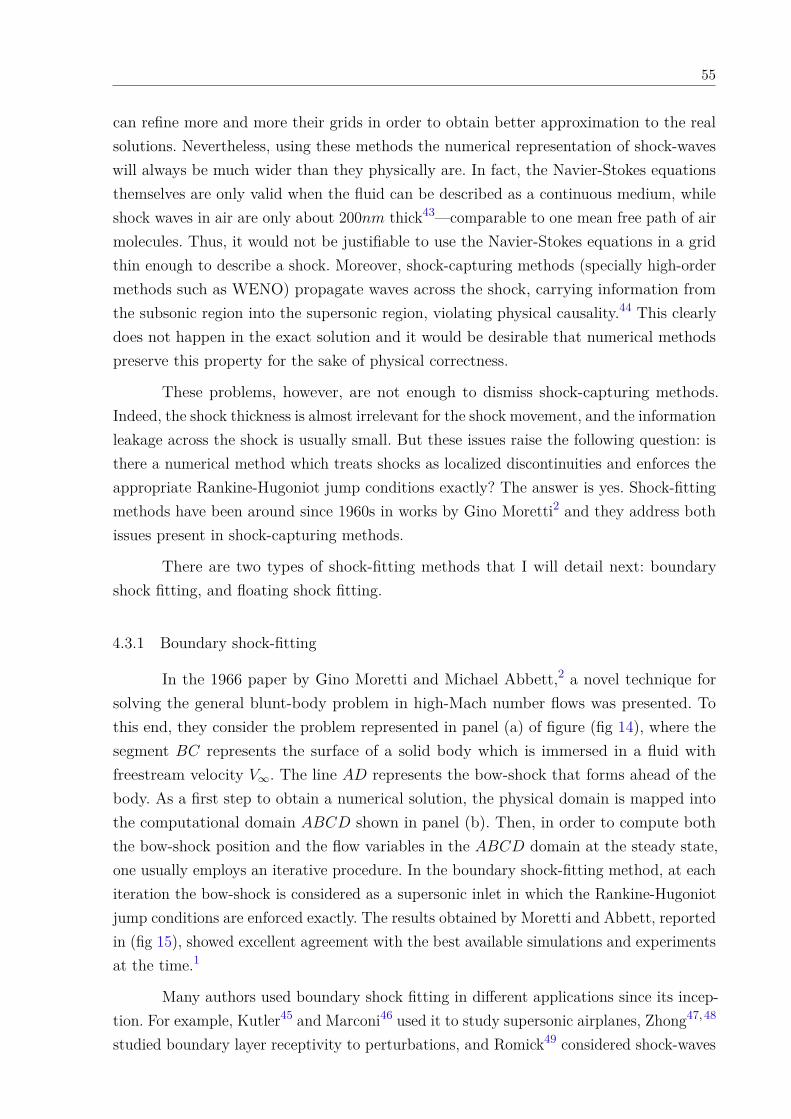
55
can refine more and more their grids in order to obtain better approximation to the realsolutions. Nevertheless, using these methods the numerical representation of shock-waveswill always be much wider than they physically are. In fact, the Navier-Stokes equationsthemselves are only valid when the fluid can be described as a continuous medium, whileshock waves in air are only about 200nm thick43—comparable to one mean free path of airmolecules. Thus, it would not be justifiable to use the Navier-Stokes equations in a gridthin enough to describe a shock. Moreover, shock-capturing methods (specially high-ordermethods such as WENO) propagate waves across the shock, carrying information fromthe subsonic region into the supersonic region, violating physical causality.44 This clearlydoes not happen in the exact solution and it would be desirable that numerical methodspreserve this property for the sake of physical correctness.
These problems, however, are not enough to dismiss shock-capturing methods.Indeed, the shock thickness is almost irrelevant for the shock movement, and the informationleakage across the shock is usually small. But these issues raise the following question: isthere a numerical method which treats shocks as localized discontinuities and enforces theappropriate Rankine-Hugoniot jump conditions exactly? The answer is yes. Shock-fittingmethods have been around since 1960s in works by Gino Moretti2 and they address bothissues present in shock-capturing methods.
There are two types of shock-fitting methods that I will detail next: boundaryshock fitting, and floating shock fitting.
4.3.1 Boundary shock-fitting
In the 1966 paper by Gino Moretti and Michael Abbett,2 a novel technique forsolving the general blunt-body problem in high-Mach number flows was presented. Tothis end, they consider the problem represented in panel (a) of figure (fig 14), where thesegment BC represents the surface of a solid body which is immersed in a fluid withfreestream velocity V∞. The line AD represents the bow-shock that forms ahead of thebody. As a first step to obtain a numerical solution, the physical domain is mapped intothe computational domain ABCD shown in panel (b). Then, in order to compute boththe bow-shock position and the flow variables in the ABCD domain at the steady state,one usually employs an iterative procedure. In the boundary shock-fitting method, at eachiteration the bow-shock is considered as a supersonic inlet in which the Rankine-Hugoniotjump conditions are enforced exactly. The results obtained by Moretti and Abbett, reportedin (fig 15), showed excellent agreement with the best available simulations and experimentsat the time.1
Many authors used boundary shock fitting in different applications since its incep-tion. For example, Kutler45 and Marconi46 used it to study supersonic airplanes, Zhong47,48
studied boundary layer receptivity to perturbations, and Romick49 considered shock-waves

56
(a) A blunt body in a high-Mach number flow. (b) Computational domain repre-sentation after a coordinatetransformation.
Figure 14 – Panel (a) shows a solid body (segment BC) in a high-Mach number flow (V∞/c∞ > 1).The body abscissa b is a given fixed function. The shock abscissa s is a function of timeand y that we want to determine. A coordinate transformation f : (x, y)→ (ζ, Y )maps the physical domain in (a) into the computational domain in (b).Source: (a) and (b) ABBETT 2
Figure 15 – Solution for the flow around a circular cylinder body obtained using the boundaryshock-fitting method (the x and y coordinates are rescaled by R = ln ρ). The dotsand the dashed line were obtained by Belotserkivskii1 and were used for comparisonby Abbett and Moretti.2Source: ABBETT 2

57
emanating from high-explosives detonations. Modern implementations of this method, seeZhong48 and Romick49, introduced improved grid descriptions, new ways to compute shockvelocities using the Rankine-Hugoniot jump conditions, and can also simulate the fulltime evolution of the system. Yet, they are conceptually the same as the one implementedby Abbett and Moretti in 1966. In Rawat and Zhong’s paper 50 there is a comparison ofvarious boundary shock-fitting methods.
Let us stress that boundary shock fitting solves two important problems thatshock-capturing methods have. First, the shock is sharp, as there is no need for numericaldissipation across the domain boundary, and the correct jump conditions are appliedexactly. Second, there is no computational power wasted on the supersonic region of theflow, where all flow variables are constant. Computations are only made where necessary.
It is not always possible to identify shock waves with a domain boundary though.A second type of shock fitting was also developed by Moretti51 and that is the topic of thenext section.
4.3.2 Floating shock-fitting
Soon after developing the boundary shock-fitting method, Moretti went further anddeveloped methods capable of tracking the shock discontinuities. First, in 1969, he studiedpiston-driven flows,51 where a gas initially at rest in a tube is suddenly compressed by amoving piston. These settings are simple enough to allow for analytical solutions which canthen be compared to the numerical results. Also the resulting flow itself is relatively simple:two regions separated by a single shock-wave. This means the numerical method employedcan also be relatively simple. Moretti ends this paper stating that the treatment of flowswith multiple shocks will be found in another paper. Indeed, two years later he publishedthe aptly named paper Complicated one-dimensional flows, 52 where he showed that histechnique could handle multiple shocks, shock-shock interactions, shock-reflections andcontact discontinuities without introducing any oscillations. One of his results is presentedin (fig 16), where two moving pistons create colliding shock-waves.
Moretti continued to improve the shock-fitting method until he retired from aca-demic work. The last section in this chapter presents a simplified version of his 1983 and1987 papers on this technique.53,54
4.4 A shock-fitting method for integrating Euler equations
The mathematical structure of Euler equations is richer than what we have exploredso far. Indeed, I mentioned that flux-splitting procedures represent waves travelling indifferent directions, but this fact was not further used. Next I will explore the method ofcharacteristics for Euler equations.

58.,-»—
'-• -
15
1 EH
2
2
H
o
<
H
o
H
<
<
EH
§ H
>
O
o
CJ
g
Q
en w
2
>
o
o
E-i ft
H
2
o &
H
w §
1
^
Ei
U
>H
P
(0 Q
Q
•J W
<;
u
u
&
H
o ft
•*• o
ft 1 ft
H
1-5
§
-JC»
CM <
Ü
H
öd I
27
v
Figure 16 – Two moving pistons generating shock-waves. The thick solid lines show the pistonspaths and the shock paths. The point in the space-time diagram where shock-wavesare formed can be found analytically and are marked as hollow circles. The dashedlines are the contact discontinuities and the thin solid lines are lines of constantvelocity.Source: MORETTI52
4.4.1 Lambda scheme
The lambda scheme55 was introduced in 1979 by Moretti as an alternative toMacCormack’s method.56 I will not use the lambda scheme in any simulations reported inchapter 5, but it is useful to understand how the mathematical structure of Euler equationscan be explored to construct a numerical method.
As shown below, the lambda scheme is based on the Euler equations written interms of Riemann variables, so I start by deriving them. Consider the one-dimensionalform of (eqn 2.14), (eqn 2.15) and (eqn 2.16) with zero dissipation (qi = τij = 0):
1δ
∂c
∂t+ 1δu∂c
∂x− c∂S
∂t− cu∂S
∂x= 0 (4.27)
∂u
∂t+ u
∂u
∂x+ c
δ
∂c
∂x− c2∂S
∂x= 0 (4.28)
∂S
∂t+ u
∂S
∂x= 0. (4.29)
By defining
R1 = c
δ+ u, R2 = c
δ− u, λ1 = u+ c, λ2 = u− c, (4.30)

59
Figure 17 – Schematic representation of Riemann variables following the characteristics lines inthe space-time diagram. Black solid lines represent constant R1 and gray dashedlines represent constant R2. The blue line at the bottom is the dependency domainof the blue circle.Source: By the author.
we can rewrite (eqn 4.27), (eqn 4.28) and (eqn 4.29) as
∂R1
∂t+ λ1
(∂R1
∂x− c∂S
∂x
)− c∂S
∂t= 0 (4.31)
∂R2
∂t+ λ2
(∂R2
∂x− c∂S
∂x
)− c∂S
∂t= 0 (4.32)
∂S
∂t+ u
∂S
∂x= 0. (4.33)
The R1, R2 in (eqn 4.30) are known as Riemann variables. To understand their meaning,let’s first consider a simple case. For an isentropic flow (constant S) we obtain
∂R1
∂t+ λ1
∂R1
∂x= 0 (4.34)
∂R2
∂t+ λ2
∂R2
∂x= 0 (4.35)
with (eqn 4.33) being trivially satisfied. Then the Riemann variable R1(2) is simply beingconvected by the term ∂R1(2)/∂x. This implies that R1 and R2 are constant along thecharacteristic lines
dx
dt= λ1,
dx
dt= λ2, (4.36)
respectively. In this case R1 and R2 are called Riemann invariants. As we started withthree equations, we must also obtain three groups of characteristics. The third of themare the particle paths defined by
dx
dt= u, (4.37)
along which S is constant (in fact, in this simple case S is constant everywhere, at alltimes).
Consider the blue circle in (fig 17). The values of the Riemann variables at the bluecircle are entirely determined by the initial conditions at the domain region marked bythe blue line. The Riemann variables are therefore the fundamental information carriers inEuler equations. This is true even when the flow is no longer isentropic. By computing

60
the Riemann variables R1, R2 at any time after the initial conditions we can reconstructthe original flow variables c, u. The paths where R1, R2 are constant are not obtainedusing the simple expressions in (eqn 4.36), but the interpretation remains the same: theRiemann variable R1(2) is convected by the non-linear term ∂R1(2)/∂x− c ∂S/∂x in thepresence of the source term c ∂S/∂t.
The core of the lambda scheme is that it accounts for the above results whendiscretizing the equations of motion (eqn 4.31), (eqn 4.32) and (eqn 4.33). The scheme hasthe form of a predictor-corrector method and so it is divided in two steps. To compute atime-step from a time-level n to n + 1, for the case u > 0, the first step in the lambdascheme is computing the values fni defined as
(f1)ni =− 12∆x
([(λ1)ni + (λ1)ni−1
] [(R1)ni − (R1)ni−1
]−[(cλ1)ni + (cλ1)ni−1
] [Sni − Sni−1
])(4.38)
(f2)ni =− 12∆x
([(λ2)nj + (λ2)nj′
] [(R2)nj − (R2)nj′
]−[(cλ2)nj + (cλ2)nj′
] [Snj − Snj′
])(4.39)
(f3)ni =− 12∆x
[uni + uni−1
] [Sni − Sni−1
], (4.40)
where the sites i, j, j′ are such that j = i if λ2 > 0, j = i+1 if λ2 < 0 and j′ = j−1. Similarexpressions are obtained when u < 0. We then update the variables to an intermediatetime-level n+ 1/2 using
Sn+1/2i = Sni + (f3)ni
∆t2 (4.41)
(R1)n+1/2i = (R1)ni + [cni (f3)ni + (f1)ni ] ∆t
2 (4.42)
(R2)n+1/2i = (R2)ni + [cni (f3)ni + (f2)ni ] ∆t
2 . (4.43)
This allows to compute fn+1/2i using the intermediate values just obtained. Next, we
compute the values F n+1/2i to be used in the correction step considering the relations
(F1)n+1/2i = 2 (f1)n+1/2
i − (f1)ni−1 (4.44)
(F2)n+1/2i = 2 (f2)n+1/2
i − (f2)nj (4.45)
(F3)n+1/2i = 2 (f3)n+1/2
i − (f3)ni−1 , (4.46)
where j = i− 1 if λ2 > 0 and j = i + 1 if λ2 < 0. Finally, we use (eqn 4.41), (eqn 4.42)and (eqn 4.43) with n+ 1/2 instead of n, and F n+1/2
i instead of fni , to obtain the updatedvariables Sn+1, Rn+1
1 and Rn+12 .
4.4.2 Shock computations
In (fig 17) one can see that characteristics lines of constant R1 or R2 never crossesanother line of the same family. Of course, it is inadmissible for a point in a continuous
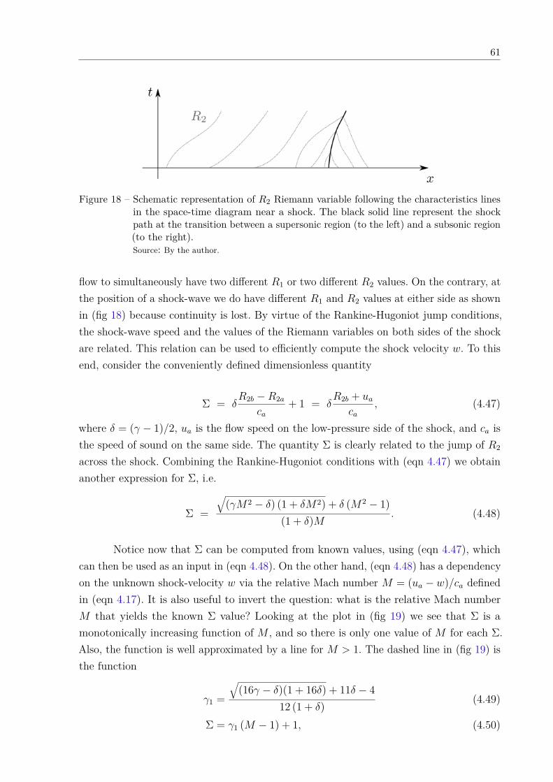
61
Figure 18 – Schematic representation of R2 Riemann variable following the characteristics linesin the space-time diagram near a shock. The black solid line represent the shockpath at the transition between a supersonic region (to the left) and a subsonic region(to the right).Source: By the author.
flow to simultaneously have two different R1 or two different R2 values. On the contrary, atthe position of a shock-wave we do have different R1 and R2 values at either side as shownin (fig 18) because continuity is lost. By virtue of the Rankine-Hugoniot jump conditions,the shock-wave speed and the values of the Riemann variables on both sides of the shockare related. This relation can be used to efficiently compute the shock velocity w. To thisend, consider the conveniently defined dimensionless quantity
Σ = δR2b −R2a
ca+ 1 = δ
R2b + uaca
, (4.47)
where δ = (γ − 1)/2, ua is the flow speed on the low-pressure side of the shock, and ca isthe speed of sound on the same side. The quantity Σ is clearly related to the jump of R2
across the shock. Combining the Rankine-Hugoniot conditions with (eqn 4.47) we obtainanother expression for Σ, i.e.
Σ =
√(γM2 − δ) (1 + δM2) + δ (M2 − 1)
(1 + δ)M . (4.48)
Notice now that Σ can be computed from known values, using (eqn 4.47), whichcan then be used as an input in (eqn 4.48). On the other hand, (eqn 4.48) has a dependencyon the unknown shock-velocity w via the relative Mach number M = (ua − w)/ca definedin (eqn 4.17). It is also useful to invert the question: what is the relative Mach numberM that yields the known Σ value? Looking at the plot in (fig 19) we see that Σ is amonotonically increasing function of M , and so there is only one value of M for each Σ.Also, the function is well approximated by a line for M > 1. The dashed line in (fig 19) isthe function
γ1 =
√(16γ − δ)(1 + 16δ) + 11δ − 4
12 (1 + δ) (4.49)
Σ = γ1 (M − 1) + 1, (4.50)

62
Figure 19 – The solid line is a plot of the function defined by (eqn 4.48). The function is almostlinear for all M > 1 values. Also, Σ > 1 if and only if M > 1. The dashed line is thefunction defined in (eqn 4.50) and is used as a first guess in the iterative procedure.Here, we considered γ = 7/5 for a diatomic gas.Source: By the author.
which coincides with the value given by (eqn 4.48) at M = 1 and M = 4.
We can now compute w with a simple iterative procedure:
(a) Compute Σ using (eqn 4.47);
(b) Obtain M from (eqn 4.50);
(c) Use M to compute Σ from (eqn 4.48) and denote it as Σ1;
(d) Update M by adding (Σ− Σ1)/γ1 to it;
(e) Iterate (c) and (d) until |Σ− Σ1| < ε, where ε is the desired accuracy;
(f) Compute w from the obtained M .
Typically only five iterations of the procedure are necessary to obtain an accuracy of 10−6.After w and M have been computed, the Rankine-Hugoniot jump conditions are simple toenforce as we can use (eqn 4.13), (eqn 4.14) and (eqn 4.15) to compute the values at thehigh-pressure side from those at the low-pressure side and the computed M . The R2 valueon the high-pressure side will be the same as before the update, but R1 and S do nothave to be preserved. Notice that in this procedure the values on the high-pressure sidechange the shock-speed w, but have no influence over the values on the low-pressure side,respecting the domain of dependency. A worked example using this procedure is shown inappendix A.
4.4.3 Shock detection
The method presented in section 2.4 detects shocks by comparing how well a regionis described by different interpolating polynomials. This means a shock will be numericallydetected shortly before being fully developed. A different method based on the ideas
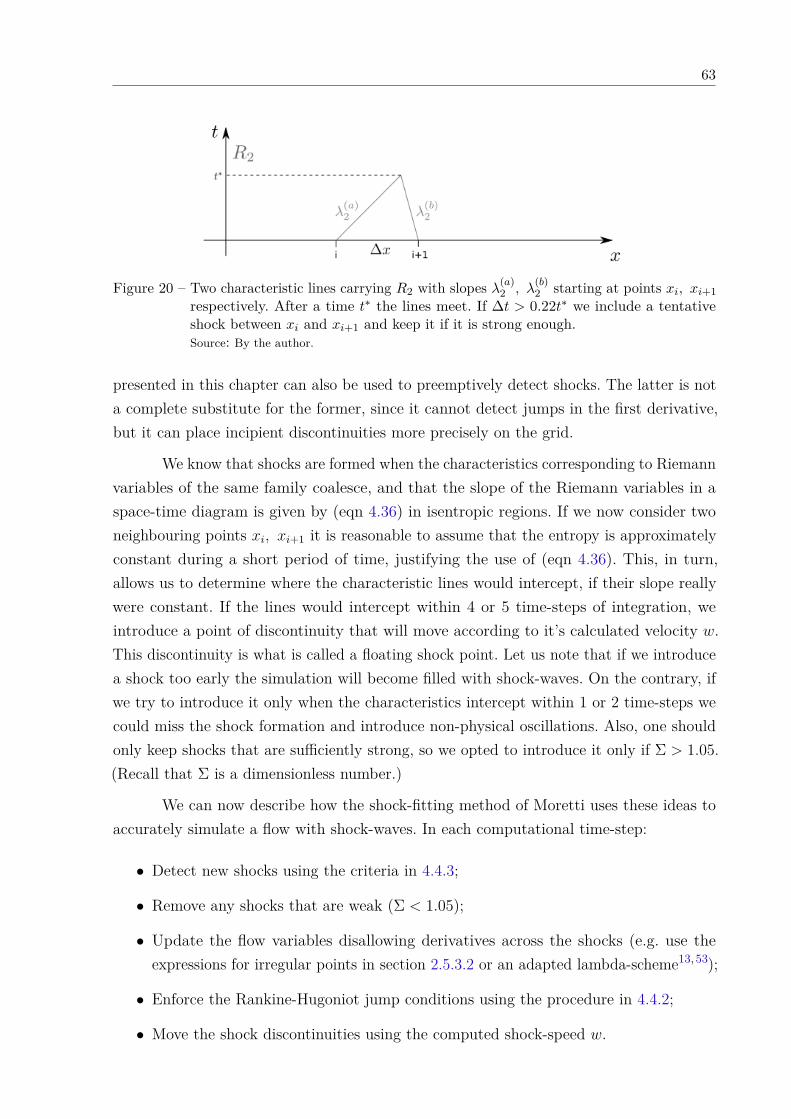
63
Figure 20 – Two characteristic lines carrying R2 with slopes λ(a)2 , λ
(b)2 starting at points xi, xi+1
respectively. After a time t∗ the lines meet. If ∆t > 0.22t∗ we include a tentativeshock between xi and xi+1 and keep it if it is strong enough.Source: By the author.
presented in this chapter can also be used to preemptively detect shocks. The latter is nota complete substitute for the former, since it cannot detect jumps in the first derivative,but it can place incipient discontinuities more precisely on the grid.
We know that shocks are formed when the characteristics corresponding to Riemannvariables of the same family coalesce, and that the slope of the Riemann variables in aspace-time diagram is given by (eqn 4.36) in isentropic regions. If we now consider twoneighbouring points xi, xi+1 it is reasonable to assume that the entropy is approximatelyconstant during a short period of time, justifying the use of (eqn 4.36). This, in turn,allows us to determine where the characteristic lines would intercept, if their slope reallywere constant. If the lines would intercept within 4 or 5 time-steps of integration, weintroduce a point of discontinuity that will move according to it’s calculated velocity w.This discontinuity is what is called a floating shock point. Let us note that if we introducea shock too early the simulation will become filled with shock-waves. On the contrary, ifwe try to introduce it only when the characteristics intercept within 1 or 2 time-steps wecould miss the shock formation and introduce non-physical oscillations. Also, one shouldonly keep shocks that are sufficiently strong, so we opted to introduce it only if Σ > 1.05.(Recall that Σ is a dimensionless number.)
We can now describe how the shock-fitting method of Moretti uses these ideas toaccurately simulate a flow with shock-waves. In each computational time-step:
• Detect new shocks using the criteria in 4.4.3;
• Remove any shocks that are weak (Σ < 1.05);
• Update the flow variables disallowing derivatives across the shocks (e.g. use theexpressions for irregular points in section 2.5.3.2 or an adapted lambda-scheme13,53);
• Enforce the Rankine-Hugoniot jump conditions using the procedure in 4.4.2;
• Move the shock discontinuities using the computed shock-speed w.


65
5 RESULTS
In this chapter, I present results obtained using some of the methods discussed inthis thesis. In no way this is a complete set of the possible results obtainable from theideas presented so far, but it is, in my opinion, a succinct demonstration of the power ofthe methods presented.
All simulations were performed on an Intel(R) Core(TM) i5-3450 CPU @ 3.10GHzusing three cores. Typical execution time for the one-dimensional simulations was 10seconds, and for the two-dimensional simulations it was about 2 hours.
5.1 One-dimensional simulations
I will first present some results for one-dimensional simulations. For this I willuse a standard test-case: Sod’s shock-tube problem.57 This problem is an instance of theRiemann problem, where two fluid regions of different densities and pressures are initiallyat rest separated by a membrane. When the membrane is removed the dynamics starts and,with the initial conditions of Sod’s shock-tube problem shown in (fig 21), a shock-waveappears. Using Euler’s equations this problem is exactly solvable through an iterativeprocedure and the solution at t = 1 can be seen in (fig 22).
Figure 21 – Initial conditions for the standard Sod’s shock-tube problem. On the left side of themembrane the fluid has ρL = 1.0, uL = 0, pL = 1.0, while it has ρR = 0.125, uR =0, pR = 0.1 on the right side. The values of e are a direct consequence of the othersquantities.Source: By the author.

66
Figure 22 – Exact results for Sod’s shock-tube problem at t = 1. Three main structures areevidenced in gray from left to right: an expansion fan, a contact discontinuity, and ashock-wave.Source: By the author.
We can now compare the results obtained for the same initial conditions usingdifferent numerical methods presented in this thesis. In particular, I will show resultsobtained using three different shock-capturing methods and results obtained using theshock-fitting method of chapter 4. A grid extending from x = −5 to x = 5 with a spacing∆x = 0.05 was used in all simulations in this section.
5.1.1 Shock-capturing
In (fig 23) I show the results obtained using the upwind flux-splitting methodpresented in 2.5.3.3. The first-order derivatives used introduce an error proportional to thesecond-derivative of the flux components. This means that regions where sharp gradientssuddenly appear, such as in contact discontinuities and shock-waves, are damped by thesecond-derivatives in the error term.
The numerical dissipation introduced by the simple first-order upwind method islarge and makes it impractical for the accuracy requirements of most practical problems.The WENO method introduces numerical dissipation in a more controlled way, as itcontinuously switches between a fifth-order method, where the flow variables change slowly,and a first-order method, in regions where they change rapidly. The result of the simulationis show in (fig 24). In particular, the WENO simulation shows a shock-wave capturedwithin fewer mesh points then in the results in (fig 23).
The main problem of the WENO method is that it is more computationallydemanding than the simple upwind method, or than methods based on central differences.As the error term in the simple upwind method is dominated by a second-order derivative,

67
Figure 23 – Results of Sod’s shock-tube problem simulated using flux-splitting technique. Somedissipative effects are evident across the contact discontinuity and the shock wave.Source: By the author.
Figure 24 – Sod’s shock-tube problem simulated using WENO convection scheme. The numericalsolution is closer to the exact solution and the discontinuities are resolved withingfewer mesh points in comparison to (fig 23).Source: By the author.

68
Figure 25 – Sod’s shock-tube problem simulated using the hybrid method. The solution is almostidentical to the one obtained using WENO method, but the use of a computationallyinexpensive method in the continuous regions makes it run about four times fasterthen a WENO simulation.Source: By the author.
this can be used in regions where the flow is smooth, since in this case the error is negligible.Therefore, one should use a method, such as the shock-detector method described in 2.5.5,that can determine the smoothness of a flow region in order to differentiate where theWENO method is necessary and where it is not. This can reduce execution time with littleto no impact on the overall method’s numerical accuracy. Let us recall that the shockdetector is able to determine the maximum derivative order Sd that can be consideredcontinuous in a region, when reconstructed using the function values at the grid points.Thus, we can use Sd as a smoothness indicator in order to decide in which regions thelower order method is acceptable. In (fig 25) we can see the results using a hybrid method,combining WENO and an upwind-biased FD scheme. Clearly they are almost identical tothose obtained using only the WENO method, but were obtained in four times less time,even considering the overhead of detecting the shocks.
To see how small is the difference between the WENO and hybrid methods, andhow they differ from the flux-splitting method I plot all three results in (fig 26).
5.1.2 Shock-fitting
Now I will show an example using the shock-fitting technique, described in section4.3.2, combined with the immersed-interface method of section 3.3. This simple proof-of-concept simulation shows the compatibility of these methods. Let us stress that thisis the first instance of a simulation using simultaneously both a shock-fitting and animmersed-interface approach.

69
Figure 26 – The three solutions discussed are compared on the same plot. The colors are thesame as in (fig 23), (fig 24) and (fig 25): flux-splitting in blue, WENO in red, and thehybrid method in green. The difference between the red and green curves is minimal.Source: By the author.
In (fig 27) we can see the density profile of a shock, with relative Mach numberM = 2, moving towards a fixed adiabatic wall (first panel). After that, the shock moveswithout spreading (second panel) and reflects from the wall (third panel). Finally, afterthe collision, the shock continues to move in the opposite direction, again without anynumerical dissipation (fourth panel).
5.2 Two-dimensional simulations
The study of one-dimensional systems such as Sod’s shock-tube in the previoussection is instructive, but not of much practical use. In this section I will show how someof the ideas presented in one-dimension can be applied to two-dimensional problems. Iwill also show examples using both immersed-interface methods described in chapter 3.All simulations in this section use the full Navier-Stokes equations.
5.2.1 Immersed-interface methods
In many points throughout this thesis I mentioned that there are many pitfalls insolving the Navier-Stokes equations. Most times an inappropriate method will generateinfinite values, or negative pressures and ultimately result in a crash, but that is not alwaysthe case. In (fig 28) we can see one such case where the simulation yields wrong resultswithout breaking down completely. This simulation uses the Ghias method, explainedin section 3.2, to describe the immersed-interface. The issue is that, when combinedwith a central-differencing scheme, as done here, numerical errors accumulate due to anodd-even decoupling between the pressure and velocity fields. Indeed, the pressure values

70
Figure 27 – Density profile of a floating-shock reflecting from a wall (black dashed line). Theinitial conditions are such that ρl = 8/3, ul = 5/4, pl = 45/14 to the left of the shock,and ρr = 1, ur = 0, pr = 5/7 to the right of it. From top to bottom the panels show:the system’s initial conditions, the shock approaching the wall, the system momentsafter the shock interacts with the wall, the shock moving away from the wall. Boththe shock and the wall boundaries are described by the same base data-structureand are treated identically when computing numerical derivatives.Source: By the author.
at odd-numbered points depend on the velocity values at the even-numbered points andvice-versa. Moreover, in these settings the viscosity is too low to ensure the coupling ofeven and odd points through the second-order derivatives. This checkerboard pattern is awell known problem in fluid simulations and a clear indication of unphysical behaviour.
On the other hand, if we use a different convection scheme, such as WENO, we canavoid the odd-even decoupling to once again obtain a physically correct solution. Indeed,in (fig 29) we can see that, when using the WENO method, the checkerboard pattern isno longer present and the solution is indeed physically acceptable.
However, using WENO or any other convection scheme is not the only way ofeliminating the unphysical oscillations. Indeed, if we apply the filter method of section2.5.4 we recouple the values of odd- and even-numbered points, avoiding the high-frequencyoscillations in the checkerboard pattern. In (fig 30) we show the result obtained using thesame central-differencing scheme considered in (fig 28) combined with this filter.
It is interesting to point out that the change in convection scheme and the use offiltering did not require any changes in the immersed-interface method being used.
As a final example in this section I also simulate the same cylinder using central-differences convection and filtering, but using Karagiozis IIM, described in 3.3, for the

71
Figure 28 – Navier-Stokes simulation of a cylinder of unit diameter at Mach number Ma = 0.5,Reynolds number Re = 500, and Prandtl number Pr = 1, performed on a 400× 200regular Cartesian grid over the domain [0, 10] × [−2.5, 2.5]. The top and bottomdomain boundaries are adiabatic no-slip walls. The left domain boundary is a subsonicinlet with a parabolic velocity profile. The right domain boundary is a subsonic outlet.The cylinder is described using Ghias IIM and convection is performed using a simplecentral-differencing scheme for all derivatives. Time evolution is obtained using thethird-order accurate Runge-Kutta scheme of section 2.5.6. The accumulation ofnumerical errors leads to an unphysical checkerboard pattern in the density field,visible in the center of the figure.Source: By the author.
boundary description instead of Ghias IIM. The results in (fig 31) are not completelycomparable to the others, since the Karagiozis IIM uses Dirichlet boundary conditions forthe temperature whereas Ghias IIM uses Neumann boundary conditions. Nevertheless, wecan see similar results to those obtained in (fig 30).
5.2.2 High-speed flows
I now extend the results of the hybrid method, used to obtain (fig 25), from one totwo dimensions, as introduced by myself in a recent conference.58 In particular, we detectshocks on each grid line and grid column as if they were one-dimensional grids. If a pointhas been marked as discontinuous in either direction, all convective terms are computedusing the WENO method, while, if it was considered smooth, all convective terms arecomputed using a central-difference scheme. Dissipative terms are always computed usingcentral differences. Similar to the one-dimensional version, this hybrid method selectively

72
Figure 29 – Navier-Stokes simulation of a unit diameter cylinder under the same conditionsused in (fig 28) except for the convective terms discretization scheme. Using WENOscheme for the convective terms controls the oscillations appearing in (fig 28) resultingin a physically acceptable solution.Source: By the author.
employs the more expansive WENO method where it is necessary, thus lowering the timerequired to run the simulation. The result is reported in (fig 32)

73
Figure 30 – Navier-Stokes simulation of a unit diameter cylinder under the same conditions usedin (fig 28) adding a filtering step. The filtering smoothes the solution by dampingthe high-frequency components, thus eliminating the checkerboard pattern from (fig28).Source: By the author.

74
Figure 31 – Navier-Stokes simulation of a unit diameter cylinder under the same conditionsconsidered in (fig 30) except for the immersed-interface method used to describe thecylinder. Here, the simulation was performed using Karagiozis boundary descriptionand the results are similar but not identical to those obtained in (fig 30), due to thedifference in boundary conditions at the interface. The blue jagged pattern visiblenear the interface is an artifact of plotting and it is not related to the simulationresults.Source: By the author.

75
Figure 32 – Simulation of a cylinder travelling at a Mach number Ma = 3, Reynolds numberRe = 500, and Prandtl number Pr = 1, using the hybrid method. The bow shockis well resolved and no unphysical oscillations are visible. The white lines, calledstreaklines, trace the path a particle would follow in the fluid.Source: By the author.

77
6 CONCLUSIONS
In the present thesis I have studied immersed-interface methods and methods tohandle shock-waves. The original topic of my thesis was high-performance implementationsof computational fluid dynamics methods, but it changed throughout the years. Never-theless, my study was always guided by the search for numerical methods amenable tooptimizations, such as those based on Cartesian grids, which are suitable building blocksfor high-performance computing. In particular, in this thesis, I proposed two versions ofIIMs simplifying their original implementations. Also, I have shown how one can use ashock-detector to combine a computationally-demanding shock-capturing method with afast non-conservative method, in order to reduce simulations run-time. Finally, I combineda shock-fitting method and an IIM. Such combination can accurately position a shock-waveon the grid and account for shock-shock and shock-wall interactions using fewer gridpoints. Next, I will summarise the main results and suggest ways in which this work canbe continued.
The first new result in this thesis was the simulation using a hybrid method reportedin (fig 25). By using a shock-detector to switch between WENO method and a FD scheme,I obtained almost identical results as the ones computed using WENO method exclusively,but in less time. I have also extended this result to two dimensions in (fig 32). There aresome minor disadvantages to this method, though. First, depending on the combinationof methods employed almost all points in the grid are marked as discontinuous and allbenefits are lost. Second, it is not obvious what should be the shock-detector sensitivity, i.e.the value of Sd that triggers the switching, so there is a tunable parameter to be adjusted.
In this work, Ghias immersed-interface method had it’s ghost-point computationssimplified, eliminating the iterative procedure originally employed when the values at oneghost-point depended directly on another’s value. This simplification did not impact themethod’s applicability compared to the original one. I showed that it can immediately becombined with both filtering methods and shock-detectors, as well as with different con-vection schemes. The main disadvantage of this IIM is the expansive computation requiredto handle moving boundaries, as the ghost-points must be determined and all image-pointpositions must be recomputed at each timestep. Karagiozis IIM, on the other hand, canhandle moving boundaries easily, as there are no auxiliary structures, e.g. image points,that need to be recomputed due to the interface moving. The original implementation ofthis second IIM required an implicit computation to obtain the dissipative terms near theinterface, but I showed that it suffices to use the second-order derivatives described insection 2.5.3.2.

78
In chapter 4 the main topic was shock waves and how they can be treated bothanalytically and numerically. I proceeded to show an alternative approach that imposes theRankine-Hugoniot jump conditions exactly: the floating shock-fitting method introducedby Gino Moretti. Moretti’s method is relatively unknown and I believe it deserves moreattention, so I joined the efforts of his close collaborators to spread it. To give mycontribution to the development of floating shock-fitting methods, I showed that the IIMcreated by Karagiozis is compatible with Moretti’s method. Indeed, both methods use thesame type of structure to mark discontinuities on the grid lines. It has been the first timea shock-fitting method was combined with an IIM. The next obvious step is to extend theresults to two dimensions.
This thesis has been my contribution to the development of fluid dynamics sim-ulation, specially by showing the viability of the shock detector of section 2.5.5 for twodimensional problems and the combination of shock-fitting and immersed interface methodsin section 5.1.2.

79
REFERENCES
1 BELOTSERKOVSKII, O. M. Flow past a circular cylin-der with a detached shock wave. 1959. Available from:<https://apps.dtic.mil/dtic/tr/fulltext/u2/607641.pdf>. Accessible at: 23 Jan.2018.
2 ABBETT, M. et al. A time-dependent computational method for blunt body flows.AIAA Journal, v. 4, n. 12, p. 2136–2141, 1966. doi: 10.2514/3.3867.
3 HALL, A.E.; CANNELL, G.H.; LAWTON, H.W. Agriculture in Semi-AridEnvironments. New York: Springer, 2011. (Ecological studies, 34).
4 PASCAL, B. Traités de l’equilibre des liqueurs et de la pesanteur de lamasse de l’air . Paris: Gauthier-Uillars, 1663. 258 p.
5 EULER, L. Principes généraux du mouvement des fluides. Mémoires de l’Académiedes Sciences de Berlin, v. 11, p. 274–315, 1757.
6 NAVIER, C. L. Memoire sur les lois du mouvement des fluides. Mémoires del’Académie des sciences de l’Institute de France, v. 6, p. 389–440, 1822.
7 SACKMANN, M. et al. Shock-wave lithotripsy of gallbladder stones. New Englandjournal of medicine, v. 318, n. 7, p. 393–397, 1988. doi: 10.1056/NEJM198802183180701.
8 SPEED, C. et al. Extracorporeal shock wave therapy for plantar fasciitis. a doubleblind randomised controlled trial. Journal of Orthopaedic Research, v. 21, n. 5, p.937–940, 2003. doi: 10.1016/S0736-0266(03)00048-2.
9 PLETCHER, R. et al. Computational fluid mechanics and heat transfer, 2nded. Washington: Taylor & Francis, 1997.
10 OBSERVATORY, E. von Karman Vortices. 2002. Available from <https://earthobservatory.nasa.gov/images/2613/von-karman-vortices>. Accessible at: 10 Dec.2018.
11 DYKE, M. V. An album of fluid motion. California: Parabolic Press, 1982.
12 STOKES, G. G. On the theories of the internal friction of fluids in motion.Transactions of the Cambridge Philosophical Society, VIII, p. 287–305, 1845.
13 NASUTI, F. et al. Analysis of unsteady supersonic viscous flows by a shock-fittingtechnique. AIAA Journal, v. 34, n. 7, p. 1428–1434, 1996. doi: 10.2514/3.13249.
14 GINGOLD, R. A. et al. Smoothed particle hydrodynamics: theory and application tonon-spherical stars. Monthly Notices of the Royal Astronomical Society, v. 181,n. 3, p. 375–389, 1977. doi: 10.1093/mnras/181.3.375.
15 CHEN, S. et al. Lattice Boltzmann method for fluid flows. Annual review of fluidmechanics, v. 30, n. 1, p. 329–364, 1998. doi: 10.1146/annurev.fluid.30.1.329.

80
16 HUSSAINI, M. Y. et al. Spectral methods in fluid dynamics. Annual Review ofFluid Mechanics, v. 19, n. 1, p. 339–367, 1987. doi: 10.1146/annurev.fl.19.010187.002011.
17 JAVADI, A. et al. Modification of k-epsilon turbulent model using kineticenergy–preserving method. Numerical Heat Transfer, v. 68, n. 6, p. 554–577, 2015.doi: 10.1080/10407790.2015.1065145.
18 MANISHA, P. Multiblock mesh. 2014. Available from <https://manisha059.files.wordpress.com/2014/01/super-fine-mesh.png>. Accessible at: 16 Mar. 2019.
19 CHEN, X. Unstructured mesh. 2011. Available from <https://www.msi.umn.edu/~chenxy/images/msh4.gif>. Accessible at: 18 Mar. 2019.
20 MORTON, K. et al. Numerical solution of Partial differential equations. NewYork: Cambridge University Press, 2005.
21 ANDERSON, J. et al. Computational fluid dynamics: an introduction. NewYork: Springer Berlin Heidelberg, 2013.
22 GIBBS, J. W. Fourier’s series. Nature, v. 59, n. 1522, p. 200, 1898. doi:10.1038/059200b0.
23 . Fourier’s series. Nature, v. 59, n. 1539, p. 606, 1899. doi: 10.1038/059606a0.
24 CARSLAW, H. S. A historical note on gibbs’ phenomenon in fourier’s series andintegrals. Bulletin of the American Mathematical Society, v. 31, n. 8, p. 420–424,1925. doi: 10.1090/S0002-9904-1925-04081-1.
25 STEGER, J. L. et al. Flux vector splitting of the inviscid gasdynamic equations withapplication to finite-difference methods. Journal of Computational Physics, v. 40, p.263–293, 1981. doi: 10.1016/0021-9991(81)90210-2.
26 LIU, X.-D. et al. Weighted essentially non-oscillatory schemes. Journal ofcomputational physics, v. 115, p. 200–212, 1994. doi: 10.1006/jcph.1994.1187.
27 VASILYEV, O. V. et al. A general class of commutative filters for LES in complexgeometries. Journal of Computational Physics, v. 146, n. 1, p. 82–104, 1998. doi:10.1006/jcph.1998.6060.
28 OLIVEIRA, M. L. B. de et al. Analysis of a high-order finite difference detector fordiscontinuities. International Journal of Computer Mathematics, v. 94, n. 2, p.676–689, 2016. doi: 10.1080/00207160.2015.1124100.
29 HYMAN, M. A. Non-iterative numerical solution of boundary-value problems.Applied Scientific Research B, Springer, v. 2, n. 1, p. 325–351, 1952. doi:10.1007/BF02919780.
30 LEVEQUE, R. J. et al. The immersed interface method for elliptic equationswith discontinuous coefficients and singular sources. SIAM Journal on NumericalAnalysis, v. 31, n. 4, p. 1019–1044, 1994.
31 LI, Z. The immersed interface method: a numerical approach for partialdifferential equations with interfaces. 1994. 172 p. Ph. D. Thesis (Philosophy) – Universityof Washington, Washington, 1994.

81
32 LI, Z. An overview of the immersed interface method and its applications. TaiwaneseJournal of Mathematics, v. 7, n. 1, p. 1–49, 2003. doi: 10.11650/twjm/1500407515.
33 ZHONG, X. A new high-order immersed interface method for solving elliptic equationswith imbedded interface of discontinuity. Journal of Computational Physics, v. 225,n. 1, p. 1066–1099, 2007. doi: 10.1016/j.jcp.2007.01.017.
34 PESKIN, C. Flow patterns around heart valves: A numerical method. Journal ofComputational Physics, v. 10, n. 2, p. 252–271, 1972. doi: 10.1016/0021-9991(72)90065-4.
35 GHIAS, R. et al. A sharp interface immersed boundary method for compressibleviscous flows. Journal of Computational Physics, v. 225, n. 1, p. 528–553, 2007. doi:10.1016/j.jcp.2006.12.007.
36 KARAGIOZIS, K. et al. A low numerical dissipation immersed interface method forthe compressible Navier-Stokes equations. Journal of Computational Physics, v. 229,n. 3, p. 701–727, 2010. doi: 10.1016/j.jcp.2009.10.005.
37 WEISSTEIN, E. W. Cubic spline. Available from <http://mathworld.wolfram.com/CubicSpline.html>. Accessible at: 26 Jan. 2019.
38 SHIN, J. et al. Reflection coefficients and reflected scaled impulses from detonations ofhigh explosives as a function of angle of incidence. Journal of Structural Engineering,v. 143, n. 7, p. 04017043, jul 2017. doi: 10.1061/(asce)st.1943-541x.0001766.
39 SALAS, M. D. A shock-fitting primer. Boca Raton: CRC Press, 2017. (Chapman& Hall/CRC Applied Mathematics & Nonlinear Science).
40 WU, Z. et al. Review of shock wave detection method in CFD post-processing.Chinese Journal of Aeronautics, v. 26, n. 3, p. 501–513, jun 2013. doi:10.1016/j.cja.2013.05.001.
41 LEVEQUE, R. J. et al. Numerical Methods for Conservation Laws. Basel:Birkhäuser, 2005.
42 GOTTLIEB, S. et al. Recovering high-order accuracy in WENO computations ofsteady-state hyperbolic systems. Journal of Scientific Computing, v. 28, n. 2-3, p.307–318, 2006. doi: 10.1007/s10915-006-9078-8.
43 TALBOT, L. et al. Measurement of shock wave thickness by the electron beamfluorescence method. Physics of Fluids, v. 9, n. 4, p. 633, 1966. doi: 10.1063/1.1761728.
44 MORETTI, G. Thirty-six years of shock fitting. Computers & Fluids, v. 31, p.719–723, 2002. doi: 10.1016/S0045-7930(01)00072-X.
45 KUTLER, P. et al. Multishocked, three-dimensional supersonic flowfields with realgas effects. AIAA Journal, v. 11, n. 5, p. 657–664, 1973. doi: 10.2514/3.50505.
46 MARCONI, F. et al. Computation of three dimensional flows about aircraftconfigurations. Computer & Fluids, v. 1, n. 2-3, p. 185–195, 1973. doi: 10.1016/0045-7930(73)90017-0.

82
47 ZHONG, X. High-order finite-difference schemes for numerical simulation ofhypersonic boundary-layer transition. Journal of Computational Physics, v. 144,n. 2, p. 662–709, 1998. doi: 10.1006/jcph.1998.6010.
48 . Leading-edge receptivity to free-stream disturbance waves for hypersonic flowover a parabola. Journal of Fluid Mechanics, v. 441, n. 2001, p. 315–367, 2001. doi:10.1017/S0022112001004918.
49 ROMICK, C. M. et al. High-order shock-fitted detonation propagation in highexplosives. Journal of Computational Physics, v. 332, p. 210–235, 2017. doi:10.1016/j.jcp.2016.11.049.
50 RAWAT, P. S. et al. On high-order shock-fitting and front-tracking schemes fornumerical simulation of shock-disturbance interactions. Journal of ComputationalPhysics, v. 229, n. 19, p. 6744–6780, 2010. doi: 10.1016/j.jcp.2010.05.021.
51 MORETTI, G. A Critical Analysis of Numerical Techniques: ThePiston-Driven Inviscid Flow. A critical analysis of numerical techniques: thepiston-driven inviscid flow. New York, 1969. Available from: <https://apps.dtic.mil/dtic/tr/fulltext/u2/693037.pdf>. Accessible at: 23 Jan. 2019.
52 . Complicated one-dimensional flows. New York, 1971. Available from:<https://pdfs.semanticscholar.org/147b/c8d5c79c30c572aac99b31fa689904b7696f.pdf>.Accessible at: 23 Jan. 2019.
53 MORETTI, G. et al. An improved lambda-scheme for one-dimensional flows.Washington: National Aeronautics and Space Administration, 1983. (NASA contractorreport, 3712).
54 MORETTI, G. A technique for integrating two-dimensional Euler equations.Computers and Fluids, v. 15, n. 1, p. 59–75, 1987. doi: 10.1016/0045-7930(87)90005-3.
55 . The λ-scheme. Computers & Fluids, v. 7, n. 3, p. 191–205, 1979. doi:10.1016/0045-7930(79)90036-7.
56 MACCORMACK, R. The effect of viscosity in hypervelocity impact cratering.In: AERODYNAMIC TESTING CONFERENCE, 4., 1969. doi: 10.2514/6.1969-354.
57 SOD, G. A. A survey of several finite difference methods for systems of nonlinearhyperbolic conservation laws. Journal of Computational Physics, v. 27, n. 1, p. 1–31,1978. doi: 10.1016/0021-9991(78)90023-2.
58 AURICHIO, V. H. et al. An immersed interface method for high mach number flowsIn: CONGRESSO BRASILEIRO DE FLUIDODINÂMICA COMPUTACIONAL, 2., 2018.Rio de Janeiro. Anais... Rio de Janeiro: Galoa, 2018. doi: 10.17648/cbcfd-83728.

Appendix


85
APPENDIX A – A WORKED SHOCK-COMPUTATION EXAMPLE
I will show how the procedure described in 4.4.2 is used to enforce the Rankine-Hugoniot jump conditions. We will consider the same initial conditions used in (fig 27),i.e. ρa = 1, ua = 0, pa = 5/7 and ρb = 8/3, ub = 5/4, pb = 45/14, and use (fig 33) as areference. As before, we set γ = 7/5 which implies δ = (γ− 1)/2 = 1/5. Using these values,we obtain ca = 1 and cb = 3
√3/4. To compute Σ we first compute the Riemann variable
R2b = cbδ− ub = 15
√3
4 + 54 , (A.1)
and then we obtain Σ using (eqn 4.47), i.e.
Σ = δR2b + ua
ca= 3√
3 + 14 . (A.2)
We have to remember that Σ is computed in a reference frame directed from the low-pressure side a towards the high-pressure side b, so that the velocity ub had it’s signflipped. If we use the iterative procedure in 4.4.2 to determineM we obtainM = 2. Indeed,substituting M = 2 in (eqn 4.48) we find the same value for Σ as in (eqn A.2). Notice thatto obtain M we used only one quantity from the high-pressure side b, namely R2b, and soany other combination of ρb, ub and pb resulting in the same value of R2b would give thesame value forM . UsingM = 2 we can now obtain the shock-velocity w = uA−Mca = −2.Again, recall that the reference frame is reversed, so the shock is moving from left to right.Finally, using (eqn 4.7), (eqn 4.8) and (eqn 4.10) we can compute the values for ρb, ub andpb from the flow-variable values in a and w. In this example, they would be the same as inthe initial conditions.
Figure 33 – Schematic view of a shock. The low-pressure side a is on the right and the high-pressure side b to the left of the shock. The reference frame for the shock computationis the normal unit vector n.Source: By the author.