1

IMF arrangements, politics and the timing of stabilizations *

Francisco José Veiga**

Núcleo de Investigação em Políticas Económicas (NIPE)

Universidade do Minho

Abstract

This paper analyses the effects of International Monetary Fund (IMF) arrangements on

the timing of inflation stabilization programs. Essentially, we test the hypothesis that

IMF aid accelerates stabilization using probit and proportional hazards models. As in

theoretical models, results are mixed: larger withdrawals of the amounts agreed to seem

to hasten stabilization, but there is weak evidence that IMF arrangements lead to greater

delays. Concerning other effects, greater fragmentation of the political system delays

stabilization while higher inflation tends to hasten it. Other political and economic

variables do not seem to have significant effects on the timing of stabilizations.

Keywords: IMF, stabilization, timing, politics.

* The author wishes to express his gratitude for the financial support of the Portuguese Foundation for Science and Technology (FCT) under research grant POCTI/32491/ECO/2000. This paper also benefited from the efficient research assistance of Vítor Castro and Paula Martins. ** Francisco José Veiga Escola de Economia e Gestão, Universidade do Minho P-4710-057 Braga - Portugal Tel: +351-253604534; Fax: +351-253676375; E-mail: fjveiga@eeg.uminho.pt

2

1. Introduction

This paper analyses the effects of International Monetary Fund (IMF)

arrangements on the decision to implement stabilization programs in countries suffering

from chronic inflation. Essentially, we test the hypothesis that IMF aid accelerates

stabilization. By providing financial means that may allow the reduction of inflation

without incurring politically unacceptable economic costs, foreign aid can hasten

stabilization. But, since aid can also reduce the costs of inflation, it may eventually

delay the necessary reforms. This is likely to happen when the most influential interest

groups do not agree on the need for reform or on how it should be conducted. Thus, the

effects of aid may depend on the timing of its announcement and its transfer.

In this paper, the information available since the late 1950s on IMF

arrangements with 10 countries that suffered from chronic inflation is used to construct

a series of variables describing amounts agreed to and the timing of announcements and

transfers. Several political and economic variables are also included in the estimations:

degree of fragmentation of the political system, ideological orientation of the

government, time in office, whether the political system is a democracy or a

dictatorship, inflation rate, government budget balance, GDP growth, stock of foreign

exchange reserves, etc.

Probit and proportional hazards models are used to evaluate the effects of those

explanatory variables on the probability of starting a stabilization program in a situation

of high inflation. Results are mixed: although the percentage drawn of the amounts

agreed to is positively related to the speed of implementation of a stabilization program,

the existence of an arrangement with the IMF may delay it. The amounts agreed to and

the duration of the arrangements do not seem to matter. As found in Veiga (2000),

greater fragmentation of the political system delays stabilization while higher inflation

3

tends to hasten it. Other political and economic variables do not seem to have

significant effects.

2. Delayed Stabilization

One intriguing fact that is common to countries that have suffered from chronic

inflation is that they followed unsustainable monetary and fiscal policies for long

periods of time. Even when policymakers recognized that these policies were

suboptimal, they tended to take too long to reverse them and implement the necessary

stabilization programs.

Assuming an unreasonable degree of myopia or irrationality of policymakers is

not a desirable way to explain delays, as it offers no constructive explanation of the

phenomenon. Thus, one can either assume that the timing of stabilizations is the rational

and deliberate choice of a policymaker maximizing a social welfare function, or that

policy choices result from negotiations between contending interest groups and delays

are caused by difficulty in reaching agreements. The rest of this section describes some

of the models based on these assumptions.1

Orphanides (1996) presents a model in which the delay and abandonment of a

stabilization program are possible decisions of a policymaker who tries to maximize a

social welfare function. A program can be delayed when more favourable initial

conditions are expected, or abandoned when the expected gains of reducing inflation are

lower than stabilization costs. In this model, a more severe inflation is likely to hasten

stabilization and, if a prospective reform is to be accomplished via the management of

the exchange rate, the level of foreign reserves (subject to stochastic shocks) will be a

1 For more complete descriptions of these models see Drazen (1996) and Veiga (2000).

4

critical factor. Thus, low levels of foreign reserves may result in delayed or abandoned

stabilization programs.

Alesina and Drazen (1991) present a political economy model in which delays

of stabilizations result when two groups with conflicting interests do not agree on the

distribution of the costs of stabilization. This “war of attrition” ends when one of the

groups concedes, that is, accepts paying a higher proportion of the taxes needed to

eliminate the deficit. In this model, one important factor leading to delays is the degree

of political polarization among interest groups. Drazen and Grilli (1993) and Hsieh

(2000) extend this model, emphasizing the possible benefits of adverse exogenous

shocks or crises that may hasten stabilization. In this context, very high inflation results

in higher costs of delaying stabilization, which should lead to its earlier implementation.

Political instability and polarization are the key factors leading to an excessive

use of seigniorage in the model of Cukierman, Edwards and Tabellini (1992). When

incumbent policymakers face a small probability of re-election and have different

preferences from the prospective winners, they are induced to delay reform and leave an

inefficient tax system to their successors. Their empirical results show that countries

with more unstable political systems tend to rely more on seigniorage.

Interest groups are generally represented by political parties. Thus, fragmented

political systems, generally with many parties represented in parliament, tend to be

associated with a high degree of political polarization and instability.2 In the models

discussed above, this would lead to greater delays of stabilizations.

To the best of our knowledge, Veiga (2000) represents the only attempt at

empirically testing these models. This paper identifies several testable hypotheses of the

2 Mainwaring and Scully (1995, pp. 28-33) argue that the most polarized political systems in Latin

America are also the most fragmented.

5

models explaining stabilization delays and tests them for 10 countries that suffered from

chronic inflation. The main conclusions are that higher fragmentation of the political

system leads to delays of stabilizations, while higher inflation hastens them. These

results provide evidence in favour of Alesina and Drazen (1991), Cukierman, Edwards

and Tabellini (1992), Drazen and Grilli (1993), and Hsieh (2000). Little or no evidence

is found of political business cycles, partisan effects, or of Orphanides’ (1996)

hypothesys that the timing of stabilization depends of the level of foreign reserves.

In a different approach, that focuses on the results of implemented programs,

Ball and Rausser (1995) investigate the effects of the key variables of the above-

mentioned models on the success of stabilization. They conclude that political

repression is not effective, political instability is detrimental, severe crises enhance the

political consensus needed for reform, and that IMF support can undermine the

credibility of stabilization programs.

3. The effects of foreign aid

The economics literature does not present a consensual view of the effects of

external aid on the timing of stabilization. On one hand, the inflow of foreign currency

will reduce the costs of stabilization and increase its probability of success, inducing

policymakers to stabilize sooner. But, on the other hand, financial assistance also

reduces the costs of living with high inflation, possibly leading to greater delays.

Orphanides (1996) analyzes the effects of external aid and conditionality in his

model. When a program is already under way, aid can increase the willingness of the

government to conclude it successfully. If the government is contemplating the

implementation of a stabilization, then programs that would be optimally delayed may

now start sooner, and programs that would start even without aid will now have a

6

greater probability of success or become less painful. The tradeoff between the

probability of success and the cost of adjustment could then be a rationale for

conditionality. Finally, the expectation of external aid in the future would lead to greater

delays of stabilizations or to the abandonment of programs already under way.

Casella and Eichengreen (1996) introduce foreign aid into the Alesina and

Drazen (1991) model. Since they assume that aid is not extended instantaneously upon

the advent of high inflation, its effects hinge precisely on the issue of timing. They find

that aid that is agreed upon and announced early and dispensed rapidly can hasten

stabilization, while aid offered late will have the opposite effect. In a “war of attrition”

game, aid announced early accelerates the transmission of information, leading to an

earlier concession by the loser, while aid that is announced late in the game will only

serve to provide the interest groups with additional resources that allow them to keep

fighting for a longer period of time. Furthermore, long intervals between the

announcement and the disbursement of aid will tend to increase delays. This happens

because the announcement of aid provides an incentive to postpone concessions until

financial assistance arrives. The greater the amount of the transfer, the more important it

is to get the timing right. They conclude that only aid that is decided and transferred

early enough will surely increase welfare in the receiving country.

Hsieh (2000) also analyzes the effects of foreign aid in a framework similar to

that of Alesina and Drazen (1991). He concludes that foreign aid is counterproductive

because, by reducing the costs of further delay, it will decrease the probability of an

agreement.

According to Dornbusch, Sturzenegger and Wolf (1990), external support can

contribute to the credibility of a program in two ways. First, external parties can

monitor the execution of the program when conditionality is imposed. Second, the

7

foreign exchange transferred will increase the probability of success of exchange rate

based stabilizations. Although they claim that the effectiveness of external aid is still an

open issue, they conclude that it critically eases the adjustment. Thus, by decreasing the

costs of stabilization, external support leads to its earlier implementation.

Although conditionality increases the credibility and reduces the delays of

stabilizations in the above models, Rodrik (1989) developed an imperfect information

model in which conditional assistance from international financial institutions can

undermine the credibility of reforms or stabilizations. He considers a framework in

which economic agents are unable to distinguish between a truly reform-minded

government and one that may reform just to secure the much desired foreign assistance.

In such case, the simple announcement of reform is not informative. This means that the

reform-minded government will have to go much further in order to reveal its true type

and secure some credibility for the stabilization. The increased costs of stabilization

may eventually lead to greater delays of credible stabilizations.3

Dreher and Vaubel (2001) argue that IMF lending causes moral hazard and

political business cycles. With respect to the former, they find that money growth and

budget deficits are higher the less a country has exhausted its borrowing potential in the

IMF and the more credit it has received from it. Thus, IMF support will not help

inflation stabilization. The IMF generates political business cycles by conceding more

credits in the democratic recipient countries in pre-election and post-election years.

3 Empirical results obtained by Ball and Rausser (1995) do not offer a final conclusion regarding the

effect of foreign assistance on the credibility and ultimate success of stabilization programs. Nevertheless,

they find weak evidence that countries receiving IMF support tend to have greater difficulty stabilizing.

8

4. The Data

The dataset is composed of quarterly data from the first quarter of 1957 to the

fourth quarter of 1999, for 10 countries that experienced chronic inflation and

implemented stabilization programs some time in this period. The 27 stabilization plans

considered are listed in Table 1, which also indicates the quarter of implementation, the

type, and the number of consecutive quarters of high inflation that preceded each

stabilization.

<< Insert Table 1 around here >>

The first major issue to solve when constructing the dataset was to determine

when a stabilization program had been implemented. The method consisted in searching

the economics literature for information on the starting dates of important stabilizations

undertaken in countries suffering from chronic inflation. 4 The second issue was to

determine when inflation was “high”, that is, when a stabilization program was clearly

necessary. Inflation was considered high when it was over twice the average inflation

rate of the last 10 years (and above 25%) or greater than or equal to 100%.

The list of IMF arrangements with the 10 countries included in the sample is

presented in Table 2, and the variables used in the estimations shown in this paper are

described in Table 3. The remaining variables, those that were never or seldom

statistically significant, are listed in Table 4. Since quarterly data are not always

available for some of the countries studied, straight- line interpolation was used to

generate quarterly data. The variables for which interpolation was used are real GDP

4 The major references were: Bruno, et al. (1988), Bruno, et al. (1991), Calvo and Végh (1999),

Hoffmaister and Végh (1996), Kiguel and Leviatan (1992), Pastor (1992), and Végh (1992).

9

growth and Fiscal Balance as a percentage of the GDP. Even after interpolating annual

data for these variables there are still a few missing values.

<< Insert Tables 2, 3 and 4 around here >>

5. Empirical Evidence

In this section, probit and proportional hazards models are used to evaluate the

effects of a number of variables on the probability of starting an inflation stabilization

program, in a situation of high inflation. Each inflation spell contains all the consecutive

quarters of high inflation, until a stabilization plan was implemented or inflation simply

ceased to be high. For each quarter and inflation spell the dependent variable (STAB)

takes the value of one if a stabilization plan was implemented in that quarter, and zero

otherwise. If no stabilization is implemented, STAB takes the value of zero for all the

observations in that inflation spell. The explanatory variables are related to the

countries’ political systems, macroeconomic fundamentals, and arrangements of

financial assistance from the IMF.

I start by assuming that the conditional probability that a stabilization program is

implemented at time t given that it has not been implemented before (the hazard rate)

depends only on the explanatory variables. It does not change autonomously over time

and any variation must be due to the independent variables. The explanatory variables

used in the estimations whose results are shown in the paper include:

- Frag=1 and Frag=2: dummies for the fragmentation of the political system;

- Ln(Inf): log of growth in CPI since the same quarter of the previous year;

10

- Control variables not directly related to the models described above:

- FB/GDP: Fiscal Balance as a percentage of GDP;

- GDP: real GDP growth since same quarter of previous year;

- Several variables related to arrangements with the IMF;

- Country dummies, in order to control for fixed effects.

These variables are described in Table 3. The macroeconomic variables were lagged

because the start of a stabilization program could affect their contemporaneous values.

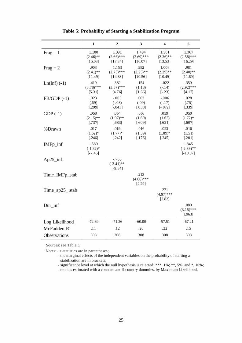
Table 5 shows the results of the five most representative estimations of the

probit model that we performed. Since the estimated coefficients are not easily

interpretable, the marginal effects of the independent variables on the dependent

variable, STAB, are also reported. They are the effects of one-unit changes in the

explanatory variables on the probability of starting a stabilization program (expressed in

percentage points) evaluated at the mean of the data. For dummy variables, they

correspond to the change in probability when the dummy changes from 0 to 1. T-

statistics for the null of no effect and the significance levels at which the null

hypotheses are rejected are also reported.

<< Insert Table 5 about here >>

Results clearly support the hypothesis that a lower fragmentation of the political

system increases the probability of starting a stabilization program (reduces delays).

Frag=1 and Frag=2 are always statistically significant and the estimated coefficients

have the expected signs. Furthermore, the estimated coefficient of Frag=1 is always

greater than that of Frag=2, as expected. This also indicates that authoritarian regimes

that did not allow political parties tend to stabilize faster. Since the most fragmented

11

political systems are generally the most unstable and polarized, these results clearly

support the conclusions of the political conflict models of Alesina and Drazen (1991)

and Cukierman, Edwards and Tabellini (1992).5

The first lag of the natural logarithm of inflation, Ln(Inf(-1)), is statistically

significant and has a positive coefficient in three estimations, providing weak support

for the benefit of crises models of Drazen and Grilli (1993) and Hsieh (2000). That is,

stabilization tends to be implemented sooner as inflation gets higher. As for the control

variables, FB/GDP(-1) is not statistically significant in the estimations shown, and

GDP(-1) has the expected sign but is statistically significant only in three estimations.

Thus, the fiscal balance does not seem to have much effect on the timing of

stabilizations, while faster GDP growth may hasten stabilization.

Some variables related to IMF arrangements were tried, with those that usually

turned out as statistically significant being described in Table 3 and included in the

estimations shown in Table 5. The percentage of the amount agreed upon with the IMF

that was drawn in a given quarter (%Drawn) is marginally statistically significant in

three estimations and has a positive sign, as expected. This implies that transferring a

large part of what was promised to a given country tends to hasten stabilization. But,

many other variables related to the amount agreed or drawn (described in Table 4) were

never or seldom statistically significant when included in the same regressions.6 Thus,

the evidence for an effect of the amounts agreed or drawn on the timing of stabilizations

is relatively weak.

5 The other political variables mentioned in Table 2 were not statistically significant when included in the

estimations. Thus, there is no support for the hypothesis that authoritarian regimes in general stabilize

faster, for partisan effects, and for political business cycles.

6 These and other results not reported in this paper are available from the author upon request.

12

An interesting result is that the existence of an arrangement with the IMF during

the current inflation spell seems to increase delays: IMFp_inf is statistically significant

and has a negative sign. When this dummy variable is equal to 1 (in the entire inflation

spell), the probability of starting a stabilization in a given quarter is reduced by 7,45

percentage points (see column 1). Ap25_inf is statistically significant and has a negative

sign. This means that the probability of starting a stabilization program also decreases

when at least 25% of the amount agreed is drawn during the current inflation spell.

These results are in line with Hsieh (2000) that argues that foreign aid is

counterproductive. But, IMFp_infq and AP25_infq, which are equal to one if the IMF

arrangement or the withdrawal occurred in the same quarter or in previous quarters of

the current inflation spell (see Table 4), are never statistically significant. Furthermore,

several other variables related to the existence or the start of an IMF program in a given

quarter or time interval (also described in Table 4), are not statistically significant. Thus,

there is at most weak evidence that the existence of an IMF arrangement increases

delays.

Contrary to our expectations, the probability of starting a stabilization increases

with the time that goes from the start of an IMF arrangement to the implementation of a

stabilization. Time_IMFp_stab is statistically significant and has a positive sign. The

same happens with Time_ap25_stab, which gives the number of quarters since at least

25% of the amount agreed was drawn until a stabilization program was implemented.

These results indicate that countries do not tend to stabilize as soon as they reach

agreement with the IMF or draw 25% of the amount agreed.

The time that goes from the onset of high inflation to the start of an IMF

arrangement or the withdrawal of 25% of the amount agreed (Time_inf_IMFp and

Time_inf_ap25) do not seem to matter. The same can be said about the time elapsed

13

between the start of an IMF arrangement and the withdrawal of 25% of the amount

agreed (Time_IMFp_ap25). These results (not shown here) are not in line with the

model of Casella and Eichengreen (1996) that attributes great importance to the timing

of the announcement and transfer of financial assistance.

Finally, the longer the number of consecutive quarters of high inflation, the

greater is the probability of starting a stabilization program: Dur_inf is statistically

significant and has a positive sign. Since the accumulated costs of high inflation grow

with the passage of time, some interest groups will eventually reach the point when the

costs of conceding are lower than those of living with high inflation, as predicted in the

Alesina and Drazen (1991) “war of attrition” model.

Table 6 shows the results when only Exchange Rate Based Stabilizations are

considered. Given the very important role of external reserves in this type of programs,

it is possible that financial assistance from the IMF becomes more important. The main

differences in comparing Tables 5 and 6 is that Ln(Inf) is no longer statistically

significant, total reserves as a percentage of imports (TR/Imp) is significant in three

estimations,7 and %Drawn is now highly statistically significant. In sum, when only

exchange rate based stabilizations are considered, the benefit of crises model of Drazen

and Grilli (1993) and Hsieh (2000) receives less empirical support, Orphanides’s (1996)

model receives weak support, as our proxy for the stock of reserves (TR/Imp) becomes

statistically significant in some estimations, and the other conclusions remain essentially

the same.

7 It should be mentioned that this variable is never statistically significant in the estimations for all 27

stabilizations (21 ERBS + 6 MBS). That is why it was excluded from the estimations shown in tables 5, 7

and 8.

14

<< Insert Table 6 around here >>

A considerable number of robustness tests not reported here was performed.

First, quarterly growth of CPI was used instead of growth of CPI since the same quarter

of the previous year. Second, growth of money since the same quarter of the previous

year was used instead of growth of the CPI. Third, current account balance as a

percentage of GDP, growth in exports, and growth in imports were added to the list of

explanatory variables, either one at a time or together. Finally, alternative definitions of

high inflation were used. The main conclusions of the analysis are unchanged in these

alternative estimations.

Probit with time dummies

As shown in tables 5 and 6, the probability of starting a stabilization plan is also

affected by the duration of high inflation: Dur_inf is statistically significant and has a

positive sign, indicating that the probability of starting a stabilization program tends to

increase with the number of consecutive quarters of high inflation.

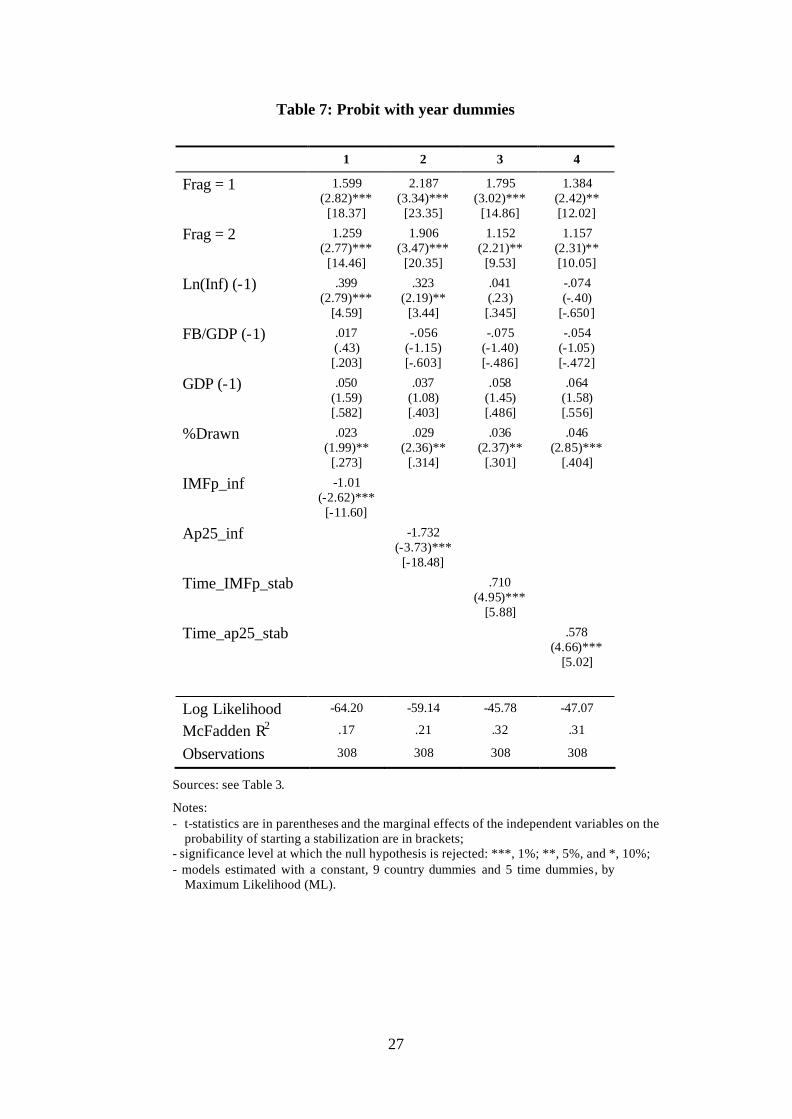
The possibility that the passage of time affects the hazard rate can also be

incorporated into the probit model by including a set of dummy variables accounting for

the duration of high inflation in the set of explanatory variables.8 In the present case, six

year dummies were created and five were included in the list of independent variables.9

8 See Allison (1982) for an example with a Logit model. He also compares the results of two Logit

models, with one assuming that the hazard rate does not change autonomously over time, and the other

relaxing that constraint by adding year dummies to the list of regressors.

9 Since the data set is composed of quarterly data, the inclusion of quarterly dummies reflecting the

duration of high inflation before stabilization would be ideal, but that was not possible because for many

15

Results are shown in Table 7.10 They are very similar to those of Table 4, with

the exception that %Drawn becomes more significant. Thus, the main conclusions

remain the same when we account for time effects by including year dummies in the

estimated models.

<< Insert Table 7 around here >>

Proportional hazards model11

While a probit model has the advantage of being easily estimated by most of the

statistical software packages available, it might not be the most correct model to apply

in the present case. Estimated coefficients are not necessarily the discrete-time

equivalent of the underlying continuous-time model and the coefficient vector is not

invariant to the length of the time intervals, meaning that the choice of quarterly data

(instead of monthly or annual data) may affect estimated coefficients.

Prentice and Gloeckler (1978) developed a discrete-time version of the

proportional hazards model that does not suffer from the problems of the probit noted

above. It is expressed as follows:

quarters there were no stabilizations being implemented. This means that the dummies for these quarters

would completely predict the value of the dependent variable (STAB=0). Thus, six yearly dummies were

created instead: 5 for the first five years of high inflation before a stabilization program started, and a 6th

for all the remaining years. The creation of additional year dummies was not possible because these

would totally predict the value of the dependent variable.

10 Since the variable Dur_inf was excluded from the set of regressors, only the results of four estimations

are shown in Table 7.

11 For descriptions of the proportional hazards model, see: Prentice and Gloeckler (1978), Allison (1982),

and Jenkins (1995).

16

( )[ ]P xit t it= − − +1 exp exp 'α β , (1)

where Pit is the probability that the inflation stabilization program i is implemented at

time t, αt is an unspecified function of time, xit is a vector of time-dependent variables

(covariates), and β is a vector of parameters which is unknown. In this model, the

discrete-time estimated coefficients are also estimates of the underlying continuous-time

model and the coefficient vector is invariant to the length of the time interval.

The estimation results obtained using the proportional hazards model are shown

in Table 8. They are similar to those of the probit model with year dummies, but the

levels of statistical significance are generally lower. The main differences occur in the

first and fourth estimations, where GDP(-1) becomes significant, and in the third

estimation, where FB/GDP(-1) is marginally significant. Nevertheless, the conclusions

regarding the support for the testable hypotheses remain essentially the same.

<< Insert Table 8 around here >>

6. Conclusions

The empirical analysis of the effects of IMF financial assistance on the timing of

stabilizations does not provide clear evidence for the hypothesis that aid accelerates

stabilization. Although he higher the percentage drawn of the amounts agreed to the

sooner stabilization will be implemented, several other variables related to the amounts

agreed to or drawn are never or seldom statistically significant. Furthermore, the

existence of an IMF arrangement during the inflation spell seems to reduce the

probability of starting a stabilization program, supporting Hsieh’s, 2000 conclusions.

Also contrary to what was expected, a longer period of time between the start of an IMF

arrangement (or the withdrawal of 25% of the amount agreed) tends to increase that

17

probability. Thus, there is no clear evidence that IMF assistance hastens stabilizations,

nor for the effects of the timing of the arrangements predicted in the model of Casella

and Eichengreen (1996). Obviously, more work is needed in this field. A natural

shortcoming of empirical studies like the present one is that it is practically impossible

to obtain data on expectations regarding the timing and amounts of foreign aid, which

are important elements of the models described in section 3.

Results regarding testable hypotheses of the models of delayed stabilizations

presented in section 2 are clearer. The hypothesis that higher fragmentation of the

political system leads to delays of stabilizations is supported by the results of probit and

proportional hazards models. Since the fragmentation of the political system is

generally associated with political instability and polarization, there is evidence in

favour of the political conflict models of Alesina and Drazen (1991) and Cukierman,

Edwards, and Tabellini (1992). There is also some support for the hypothesis that higher

inflation hastens stabilizations, as suggested by Drazen and Grilli (1993), Orphanides

(1996), and Hsieh (2000). Finally, Orphanides’ (1996) hypothesis that the decision to

implement a stabilization program is essentially based on the available amount of

foreign reserves receives weak support when only the 21 exchange rate based

stabilizations are included in the sample. When all 27 stabilizations are considered, the

stock of reserves does not affect the probability to implement a stabilization program.

In sum, financial assistance from the IMF may not matter much for the timing of

inflation stabilization programs. Actually, empirical results suggest that the structure of

the political system may play a more important role. In more fragmented political

systems, usually the most unstable and polarized, conflicts of interests between political

parties make the approval of new legislation harder and stabilization programs are often

delayed until a serious crisis sets in, regardless of whether financial assistance is

18

received or not. Thus, as suggested by political conflict models, the structure of the

political system may help explain why suboptimal policies are kept for long periods of

time and the necessary corrective actions are not taken.

References

Alesina, A. and A. Drazen, 1991, Why are stabilizations delayed? American Economic

Review 81(5), 1170-1188.

Allison, P.D., 1982, Discrete-time methods for the analysis of event histories, in:

Leinhardt, S., ed., Sociological Methodology. (Jossey-Bass Publishers, San

Francisco, CA) 61-97.

Ball, Richard and Gordon Rausser, 1995, Governance structures and the durability of

economics reforms: evidence from inflation stabilizations. World Development

23(6), 897-912.

Banks, A.C., ed., Political Handbook of the World (McGraw-Hill, New York, NY)

various issues.

Bruno, M., et al., eds., 1988, Inflation Stabilization: The Experience of Israel,

Argentina, Brazil, Bolivia, and Mexico (MIT Press, Cambridge, MA).

Bruno, M., et al., eds., 1991, Lessons of Economic Stabilization and its Aftermath (MIT

Press, Cambridge, MA).

Calvo, G.A. and C.A. Végh, 1999, Inflation stabilization and BOP crises in developing

countries, in Taylor, J.B. and M. Woodford, eds. Handbook of Macroeconomics,

Vol. 1, (Elsevier, Holland), 1531-1614.

Casella, A. and B. Eichengreen, 1996, Can foreign aid accelerate stabilization?

Economic Journal 106, 605-619.

19

Cukierman, A., S. Edwards, and G. Tabellini, 1992, Seigniorage and political

instability. American Economic Review 82(3), 537-555.

Drazen, A., 1996, The political economy of delayed reform. The Journal of Policy

Reform 1(1), 25-46.

Dornbusch, Sturzenegger and Wolf, 1990, Extreme inflation: dynamics and

stabilization. Brookings Papers on Economic Activity 2(1990), 1-64.

Drazen, A. and V. Grilli, 1993, The benefit of crises for economic reforms. American

Economic Review 83(3), 598-607.

Dreher, A. and R. Vaubel, 2001, Does the IMF cause moral hazard and political

business cycles? Evidence from panel data, IVS Working Paper nº 598-01,

University of Mannheim.

Gorvin, I., ed., 1989, Elections Since 1945: A Worldwide Reference Compendium (St.

James Press, Chicago, IL).

Hoffmaister, A.W. and C.A. Végh, 1996, Disinflation and the recession-now-versus-

recession-later hypothesis: Evidence from Uruguay. IMF Staff Papers 43(2),

355-394.

Hsieh, C.T., 2000, Bargaining over reform, European Economic Review 44, 1659-1676.

International Monetary Fund, Annual Report (IMF, Washington D.C.), several issues.

Jenkins, S.P., 1995, Easy estimation for discrete-time duration models. Oxford Bulletin

of Economics and Statistics 57(1), 129-139.

Kiguel, M., and N. Leviatan, 1992, The business cycle associated with exchange rate-

based stabilizations. The World Bank Economic Review 6(2), 279-305.

Mainwaring, S. and T.R. Scully, eds., 1995, Building Democratic Institutions: Party

Systems in Latin America (Stanford University Press, Stanford, CA).

20

McDonald, R.H. and J.M. Ruhl, 1989, Party Politics and Elections in Latin America

(Westview Press, Boulder, CO).

Orphanides, A., 1996, The timing of stabilizations. Journal of Economics Dynamics &

Control 20(1-3), 257-279.

Pastor Jr., M., 1992, Inflation Stabilization & Debt: Macroeconomic Experiments in

Peru and Bolivia (Westview Press, Boulder, CO).

Prentice, R., and L.A. Gloeckler, 1978, Regression analysis of grouped survival data

with application to breast cancer data. Biometrics 34, 57-67.

Rodrik, D., 1989, Promises, promises: credible policy reform via signalling, The

Economic Journal 99, September, 736-772.

Végh, C.A., 1992, Stopping high inflation: An analytical overview. IMF Staff Papers

39(3), 626-695.

Veiga, F.J., 2000, Delays of inflation stabilizations. Economics and Politics 12(3), 275-

295.

World Europa Yearbook (Europa Publications, London, UK), several issues.

21

Table 1: Stabilization Programs

Country Program dates and names

Type Duration of “high” inflation until

stabilization (quarters)

Argentina 1959.3 ERBS 4 1967.2 ERBS 0 1973.3 ERBS 6 1978.4 (Tablita) ERBS 15 1985.2 (Austral) ERBS 15 1990.1 (Bonex) MBS 11 1991.2 (Convertibility) ERBS 1 Bolivia 1985.3 ERBS 14 Brazil 1964:2 ERBS 4 1986:1 (Cruzado) ERBS 25 1990.2 (Collor) MBS 13 1994.3 (Real) ERBS 14 Chile 1975.2 MBS 11 1978.1 (Tablita) ERBS 0 Dominican Republic 1985.2 ERBS 4 1990.3 MBS 11 Israel 1985.3 (Shekel) ERBS 31 Mexico 1976.4 ERBS 0 1988.1 ERBS 8 Peru 1981.3 ERBS 24 1985.4 ERBS 10 1990.3 MBS 11 Turkey 1980.1 ERBS 10 Uruguay 1960.4 MBS 7 1968.2 ERBS 11 1978.4 (Tablita) ERBS 0 1990.4 ERBS 2

Sources: Bruno, et al. (1988), Bruno, et al. (1991), Calvo and Végh (1999), Hoffmaister and Végh (1996), Kiguel and Leviatan (1992), Pastor (1992), and Végh (1992).

Notes: ERBS = Exchange Rate Based Stabilization (21 in this sample); MBS = Money Based Stabilization (6 in this sample).

22

Table 2: IMF arrangements

Country Month and year of IMF arrangements

Argentina: 16 SB 2 EFF

12/58-12/59; 12/59-12/60; 12/60-12/61; 12/61-05/62; 06/62-10/63; 05/67-04/68; 04/68-04/69; 08/76-08/77; 09/77-09/78; 01/83-04/84; 12/84-05/86; 07/87-09/88; 11/89-03/91; 07/91-03/92; 03/92-03/96(EFF); 04/96-01/98; 02/98-03/00 (EFF); 03/00-03/03

Bolivia: 14 SB 1 SAF, 2 ESAF 1 PRGF

11/56-12/57; 12/57-02/59; 05/59-09/60; 07/61-07/62; 08/62-08/63; 09/63-08/64; 09/64-08/65; 09/65-11/66; 12/66-12/67; 12/67-01/69; 01/69-01/70; 01/73-01/74; 02/80-01/81; 06/86-06/87; 12/86-07/88 (SAF); 07/88-05/94 (ESAF); 12/94-09/98 (ESAF); 09/98-09/01(PRGF)

Brazil: 14 SB 1 EFF

06/58-06/59; 05/61-05/62; 01/65-01/66; 02/66-01/67; 02/67-02/68; 04/68-04/69; 04/69-02/70; 02/70-02/71; 02/71-02/72; 03/72-03/73; 03/83-02/86 (EFF); 08/88-02/90; 01/92-08/93; 12/98-12/01

Chile: 15 SB 1 EFF

04/56-03/58; 04/58-03/59; 04/59-12/59; 02/61-02/62; 02/62-02/63; 01/63-01/64; 02/64-01/65; 01/65-01/66; 03/66-02/67; 03/68-02/69; 04/69-04/70; 01/74-01/75; 03/75-03/76; 01/83-01/85; 08/85-08/89 (EFF); 11/89-11/90

Dom. Republic: 5 SB, 1 EFF

12/59-12/60; 08/64-07/65; 01/83-01/85 (EFF); 04/85-04/86; 08/91-03/93; 07/93-03/94

Israel: 3 SB 11/74-02/75; 02/75-02/76; 10/76-10/77

Mexico: 5 SB, 3 EFF

03/59-09/59; 07/61-07/62; 01/77-12/79 (EFF); 01/83-12/85 (EFF); 11/86-04988; 05/89-05/93 (EFF); 02/95-02/97; 07/99-11/00

Peru: 17 SB

4 EFF

02/54-02/58; 02/58-02/59; 03/59-02/60; 03/60-02/61; 03/61-02/62; 03/62-02/63; 03/63-02/64; 03/64-02/65; 04/65-03/66; /03/66-03/67; 08/67-08/68; 11/68-11/69 04/70-04/71; 11/77-09/78; 09/78-08/1979; 08/79-07/1980; 06/82-04/1984 (EFF); 04/84-07/85; 03/93-03/1996 (EFF); 07/96-03/99 (EFF); 06/99-05/02 (EFF)

Turkey: 17 SB

01/61-12/61; 03/62-12/62; 02/63-12/63; 02/64-12/64; 02/65-12/65; 02/66-12/66; 02/67-12/67; 04/68-12/68; 07/69-06/70; 08/70-08/71; 04/78-07/79; 07/79-06/80; 06/80-06/ 83; 06/83-03/84; 04/84-04/85; 07/94-03/96; 12/99-12/2002

Uruguay: 20 SB

06/61-06/62; 10/62-10/63; 06/66-06/67; 03/68-02/69; 05/70-05/71; 06/72-06/73; 05/75-05/76; 08/76-08/77; 09/77-09/78; 03/79-03/80; 05/80-05/81; 07/81-07/82; 04/83-04/85; 09/85-03/87; 12/90-03/92; 07/92-06/93; 03/96-03/97; 06/97-03/99; 03/99-03/00; 05/00-03/2002

Sources: IMF, IMF Annual Report, several issues, and http://www.imf.org.

Notes: When the IMF program is not a stand-by, the facility used is indicated between parentheses. The abbreviations used are the following: SB = Stand-by; EFF = Extended Fund Facility; SAF = Structural Adjustment Facility; ESAF = Enhanced Structural Adjustment Facility; PRGF = Poverty Reduction and Growth Facility

23

Table 3: Descript ion of the main Variables Used and Respective Sources

Political variables:

Dummies for the degree of fragmentation of the political system: Frag = 1 No parties allowed or exclusive one-party systems; Frag = 2 One-party majority parliamentary government; or presidential government, with

the same party in control of the parliament (with an overall majority); Frag > 2 More fragmented political systems.

Type = 1 for a military dictatorship or authoritarian government, and =0 for a democracy.

Orient - Political orientation of the government: 1 conservative, antilabor or antileft government; 2 center-right government or coalition of center-right and center-left parties; 3 center-left government; 4 socialist or populist government.

Right =1 if (Orient=1 or Orient=2), and =0 otherwise.

QLCH - Quarters since last change in government or election

Economic variables:

Ln(Inf) – Natural log of growth of CPI since the same quarter of the previous year

FB/GDP - Fiscal Balance (Government Budget Balance) as a percentage of GDP

GDP - Growth of real GDP since the same quarter of the previous year

TR/Imp - Total Reserves as a percentage of Imports

%Drawn - Percentage drawn of the amount agreed in the current IMF arrangement

IMFp_inf = 1 there is an arrangement with IMF during the current inflation spell, and =0 otherwise

Ap25_inf = 1 if during the current period of high inflation at least 25% of the total amount agreed is drawn, and =0 otherwise

Time_IMFp_stab – quarters from the start of the first IMF program in that inflation spell until stabilization

Time_ap25_stab - quarters since when at least 25% of the total amount agreed has been drawn until stabilization

Dur_inf – number of quarters since the onset of high inflation (duration of high inflation)

Sources: - Political variables: Banks A. ed., Political Handbook of the World, several issues; Gorvin

(1989); McDonald and Ruhl (1989); Mainwaring and Scully (1995); World Europa Yearbook , several issues.

- Economic variables: International Financial Statistics - IMF. Quarterly data on Real GDP was also obtained from IBGE (Brazil), INEGI (Mexico), and Végh (1992), for Chile (1977:1 to 1979:4) and Uruguay (1978:1 to 1983:4). Data on the timing of IMF arrangements was obtained from the IMF Annual Report and on the IMF web page.

24

Table 4: Other Variables related to IMF arrangements

TA_tr – Total amount agreed as a percentage of total reserves minus gold TFC - Total IMF credit and loans outstanding Drawn/tr - Amount drawn as a percentage of total reserves minus gold Drawn/yvar_tr - Amount drawn as a percentage of the yearly variation in total reserves Drawn/ca - Amount drawn as a percentage of the current account balance Drawn/finob - Amount drawn as a percentage of the Overall Balance financing Apdrawn - Accumulated percentage of the amount agreed that was drawn. Ap25 = 1 if at least 25% of the total amount agreed has been drawn, and =0 otherwise Ap50 = 1 if at least 50% of the total amount agreed has been drawn, and =0 otherwise Ap75 = 1 if at least 75% of the total amount agreed has been drawn, and =0 otherwise Apdrawn0 =1 when less than 25% of the total amount agreed has been drawn, and =0 otherwise. Apdrawn25 =1 when the percentage of the total amount agreed that was drawn in between 25% and

50%, and =0 otherwise Apdrawn50 =1 when the percentage of the total amount agreed that was drawn in between 50% and

75%, and =0 otherwise Apdrawn75 =1 when more than 75% of the total amount agreed has been drawn, and =0 otherwise

IMFprogram = 1 if there was an IMF arrangement in the same year, and =0 otherwise

IMFp4 = 1 if there was an IMF arrangement in that quarter or in one of the four previous quarters, and 0 otherwise

IMFp4 = 1 if there was an IMF arrangement in that quarter or in one of the four following quarters, and 0 otherwise

IMFp8 = 1 if there was an IMF arrangement in that quarter or in one of the four previous quarters or in one of the four following quarters, and 0 otherwise

Dur_prog - Duration of the IMF program. Number of quarters from start to finish Time_last - Number of quarters since the end of the last IMF program Time_next - Number of quarters until the start of the next IMF program IMFp_start = 1 if an arrangement with IMF begins in that quarter, and =0 otherwise IMFp_start4 = 1 if an arrangement with IMF begins in that quarter or in any of the four previous

quarters, and =0 otherwise IMFp_start4p = 1 if an arrangement with IMF begins in that quarter or in any of the four following

quarters, and =0 otherwise IMFp_start8 = 1 if an arrangement with IMF begins in that quarter, in any of the four previous

quarters or in any of the four following quarters, and =0 otherwise FA = 1 if the country has an arrangement of any kind with the IMF in that quarter, =0 otherwise Standby = 1 if the country has a Stand-By arrangement with the IMF in that quarter, =0 otherwise Eff =1 if the country has an Extended Fund Facility in that quarter, and =0 otherwise

Imfp_infq = 1 if there is an IMF arrangement in that quarter or in previous quarters of the current inflation spell, and =0 otherwise

Ap25_infq = 1 if the country has drawn at least 25% of the total amount agreed up to that quarter or up to previous quarters of the current period of high inflation, and =0 otherwise

Time_inf_IMFp - quarters from the beginning of high inflation to the start of an IMF program Time_inf_ap25 - quarters from the beginning of high inflation to when at least 25% of the total

amount agreed has been drawn Time_IMFp_ap25 - quarters from the start of an IMF program to when at least 25% of the amount

agreed has been drawn

Sources: see the description at the bottom of Table 3.

25

Table 5: Probability of Starting a Stabilization Program

1 2 3 4 5

Frag = 1 1.188 (2.46)** [15.03]

1.391 (2.66)***

[17.34]

1.494 (2.69)***

[16.07]

1.301 (2.36)** [13.53]

1.367 (2.58)***

[16.29] Frag = 2 .908

(2.41)** [11.49]

1.153 (2.73)***

[14.38]

.982 (2.25)** [10.56]

1.008 (2.29)** [10.49]

.981 (2.40)** [11.69]

Ln(Inf) (-1) .419 (3.78)***

[5.31]

.382 (3.37)***

[4.76]

.154 (1.13) [1.66]

-.022 (-.14) [-.23]

.350 (2.92)***

[4.17] FB/GDP (-1) .023

(.69) [.299]

-.003 (-.08)

[-.041]

.003 (.09) [.038]

-.006 (-.17)

[-.072]

.028 (.75) [.339]

GDP (-1) .058 (2.15)**

[.737]

.054 (1.97)**

[.683]

.056 (1.60) [.609]

.059 (1.63) [.621]

.050 (1.72)* [.607]

%Drawn .017 (1.62)* [.246]

.019 (1.77)* [.242]

.016 (1.39) [.176]

.023 (1.89)* [.245]

.016 (1.51) [.201]

IMFp_inf -.589 (-1.82)* [-7.45]

-.845 (-2.39)** [-10.07]

Ap25_inf

-.765 (-2.41)**

[-9.54]

Time_IMFp_stab

.213 (4.66)***

[2.29]

Time_ap25_ stab

.271 (4.97)***

[2.82]

Dur_inf

.080 (3.15)***

[.963] Log Likelihood -72.69 -71.26 -60.00 -57.51 -67.21

McFadden R2 .11 .12 .20 .22 .15

Observations 308 308 308 308 308

Sources: see Table 3. Notes: - t-statistics are in parentheses;

- the marginal effects of the independent variables on the probability of starting a stabilization are in brackets;

- significance level at which the null hypothesis is rejected: ***, 1%; **, 5%, and *, 10%; - models estimated with a constant and 9 country dummies, by Maximum Likelihood.

26

Table 6: Results for Exchange Rate Based Stabilizations

1 2 3 4 5

Frag = 1 1.105 (2.21)** [11.57]

1.386 (2.55)** [13.99]

1.255 (2.28)** [11.87]

1.075 (1.99)** [10.00]

1.164 (2.23)** [11.80]

Frag = 2 .972 (2.35)** [10.17]

1.287 (2.77)***

[12.99]

.858 (1.88)* [8.11]

.854 (1.89)* [7.94]

.944 (2.19)**

[9.56] Ln(Inf) (-1) .183

(1.46) [1.91]

.109 (.82) [1.10]

-.031 (-.20)

[-.297]

-.161 (-.99)

[-1.50]

.135 (1.03) [1.37]

TR/Imp (-1) .321 (2.32)**

[3.36]

.331 (2.38)**

[3.34]

.095 (.63) [.889]

.096 (.64) [.898]

.238 (1.64)* [2.41]

FB/GDP (-1) .004 (.12) [.049]

-.025 (-.61)

[-.259]

.006 (.17) [.064]

.0001 (.003) [.001]

.017 (.44) [.178]

GDP (-1) .065 (1.97)**

[.684]

.061 (1.78)* [.621]

.055 (1.47) [.525]

.059 (1.54) [.549]

.058 (1.69)* [.592]

%Drawn .030 (2.57)***

[.320]

.035 (2.87)***

[.361]

.027 (2.26)**

[.257]

.033 (2.65)***

[.311]

.029 (2.42)**

[.298] IMFp_inf -.720

(-1.90)* [-7.54]

-.806 (-2.07)**

[-8.17] Ap25_inf

-1.019 (-2.87)***

[-10.28]

Time_IMFp_stab

.177 (3.70)***

[1.67]

Time_ap25_stab

.218 (3.92)***

[2.02]

Dur_inf

.055 (2.08)**

[.559] Log Likelihood -60.76 -58.15 -53.81 -52.77 -58.42

McFadden R2 .09 .11 .14 .15 .11

Observations 308 308 308 308 308

Sources: see Table 3. Notes:

- t-statistics are in parentheses and the marginal effects of the independent variables on the probability of starting a stabilization are in brackets;

- significance level at which the null hypothesis is rejected: ***, 1%; **, 5%, and *, 10%; - models estimated with a constant and 9 country dummies, by Maximum Likelihood (ML); - there are 21 Exchange Rate Based Stabilizations in the sample.

27

Table 7: Probit with year dummies

1 2 3 4

Frag = 1 1.599 (2.82)***

[18.37]

2.187 (3.34)***

[23.35]

1.795 (3.02)***

[14.86]

1.384 (2.42)** [12.02]

Frag = 2 1.259 (2.77)***

[14.46]

1.906 (3.47)***

[20.35]

1.152 (2.21)**

[9.53]

1.157 (2.31)** [10.05]

Ln(Inf) (-1) .399 (2.79)***

[4.59]

.323 (2.19)**

[3.44]

.041 (.23) [.345]

-.074 (-.40)

[-.650] FB/GDP (-1) .017

(.43) [.203]

-.056 (-1.15) [-.603]

-.075 (-1.40) [-.486]

-.054 (-1.05) [-.472]

GDP (-1) .050 (1.59) [.582]

.037 (1.08) [.403]

.058 (1.45) [.486]

.064 (1.58) [.556]

%Drawn .023 (1.99)**

[.273]

.029 (2.36)**

[.314]

.036 (2.37)**

[.301]

.046 (2.85)***

[.404] IMFp_inf -1.01

(-2.62)*** [-11.60]

Ap25_inf

-1.732 (-3.73)***

[-18.48]

Time_IMFp_stab

.710 (4.95)***

[5.88]

Time_ap25_stab

.578 (4.66)***

[5.02]

Log Likelihood -64.20 -59.14 -45.78 -47.07

McFadden R2 .17 .21 .32 .31

Observations 308 308 308 308

Sources: see Table 3.

Notes: - t-statistics are in parentheses and the marginal effects of the independent variables on the

probability of starting a stabilization are in brackets; - significance level at which the null hypothesis is rejected: ***, 1%; **, 5%, and *, 10%; - models estimated with a constant, 9 country dummies and 5 time dummies, by

Maximum Likelihood (ML).

28

Table 8: Proportional Hazards

1 2 3 4

Frag = 1 3.46 (1.78)*

4.628 (2.27)**

3.35 (2.69)***

2.92 (1.99)**

Frag = 2 2.66 (1.66)*

3.812 (2.06)**

2.33 (2.12)**

2.40 (2.03)**

Ln(Inf) (-1) .81 (2.73)***

.607 (2.18)**

-.10 (-.38)

.-.35 (-1.11)

FB/GDP (-1) .018 (.18)

-.168 (-1.14)

-.15 (-1.73)*

-.12 (-1.22)

GDP (-1) .10 (1.78)*

.095 (1.40)

.10 (1.50)

.14 (2.10)**

%Drawn .03 (1.73)*

.047 (2.04)**

.06 (2.57)***

.09 (2.85)***

IMFp_inf -2.23 (-2.09)**

Ap25_inf

-3.659 (-2.84)***

Time_IMFp_stab

1.18 (4.87)***

Time_ap25_stab

1.10 (3.97)***

Log Likelihood -62.15 -56.67 -44.17 -44.22

McFadden R2 .30 .36 .50 .50

Observations 308 308 308 308

Sources: see Table 3.

Notes: - t-statistics are in parentheses; - significance level at which the null hypothesis is rejected: ***, 1%; **,

5%, and *, 10%; - models estimated with a constant, 9 country dummies, and 5 time

dummies, by Maximum Likelihood (ML).