Imdade Chitou, Gilles Dufrénot, Julien Esposito To cite

HAL Id: halshs-03297198https://halshs.archives-ouvertes.fr/halshs-03297198

Preprint submitted on 23 Jul 2021

HAL is a multi-disciplinary open accessarchive for the deposit and dissemination of sci-entific research documents, whether they are pub-lished or not. The documents may come fromteaching and research institutions in France orabroad, or from public or private research centers.

L’archive ouverte pluridisciplinaire HAL, estdestinée au dépôt et à la diffusion de documentsscientifiques de niveau recherche, publiés ou non,émanant des établissements d’enseignement et derecherche français ou étrangers, des laboratoirespublics ou privés.

Linking Covid-19 epidemic and emerging market OAS:Evidence using dynamic copulas and Pareto

distributionsImdade Chitou, Gilles Dufrénot, Julien Esposito

To cite this version:Imdade Chitou, Gilles Dufrénot, Julien Esposito. Linking Covid-19 epidemic and emerging marketOAS: Evidence using dynamic copulas and Pareto distributions. 2021. �halshs-03297198�

https://halshs.archives-ouvertes.fr/halshs-03297198

https://hal.archives-ouvertes.fr

Working Papers / Documents de travail

WP 2021 - Nr 38

Linking Covid-19 epidemic and emerging market OAS: Evidence using dynamic copulas and Pareto distributions

Imdade Chitou Gilles Dufrénot Julien Esposito

1

Linking Covid-19 epidemic and emerging market OAS:

Evidence using dynamic copulas and Pareto distributions 1

Imdade Chitou2, Gilles Dufrénot3, Julien Esposito2

Abstract

This paper investigates the dependence of the Option-Adjusted Spread (OAS) for several ICE BofA

Emerging Markets Corporate Plus Indexes to the outbreaks of the Covid-19 viral pandemics

between March 1, 2020, and April 30, 2021. We investigate whether the number of new cases,

the reproduction rate, death rate and stringency policies have resulted in an increase/decrease

in the spreads. We study the bivariate distributions of epidemiological indicators and spreads to

investigate their concordance using dynamic copula analysis and estimate the Kendall rank-

correlation coefficient. We also investigate the effect of the epidemiological variables on the

extreme values of the spreads by fitting a tail index derived from a Pareto type I distribution. We

highlight the existence of correlations, robust to the type of copulas used (Clayton or Gumbel).

Moreover, we show that the epidemiological variables explain well the extreme values of the

spreads.

Keywords: Covid-19, corporate spreads, pandemics, emerging economies.

JEL CODES: F37; G15; I12

1 This work was supported by French National Research Agency Grant ANR-17-EURE-0020, by the Excellence Initiative of Aix-Marseille University - A*MIDEX, and by a Grant from the Institut Louis Bachelier (Institut Europlace de Finance). 2 Faculty of Economics and Management, Aix-Marseille University. 3Corresponding author: Institut Louis Bachelier, Aix-Marseille Univ., CNRS, AMSE, Marseille, France.

2

1.- Introduction

The aim of this paper is to investigate a recognized, but never tested formally, hypothesis of a

sensitivity of emerging markets corporate spreads to epidemiological indicators of coronavirus

pandemic. Indeed, without studying the effect of epidemiological variables per se, the literature

is usually interested in the impact of Covid-19 through its effects on the decisions of financial

actors. Some authors are interested in the consequences of the crisis health context on the

investors’ choices regarding the fears they may have had about the evolution of the fundamentals

of companies (liquidity, cash flows, lower returns and stock prices, higher volatility, safe heaven

effects, spillovers, etc.). Alternatively, some researchers consider that the epidemic has

generated uncertainty, which they capture by means of aggregate indicators, such as the World

Pandemic Uncertainty index, WPUI, proposed by Ahir et al., 2018, whose effects on spreads,

volatility and returns are analyzed (see also Baker et al., 2020, Narayan and Phan, 2020).

Detailed correlation studies at a daily frequency are rare. However, the kinetics of infectious

diseases can only be adequately captured at this frequency. Moreover, the non-academic press

suggests that investors are sensitive to high-frequency epidemic signals. For example, in its

November 2020 Business news, Reuters noted that U.S. junk bond spreads narrowed on optimism

about Pfizer's COVID-19 vaccine4. Shear et al (2021), study the impact of investors' attention to

the Covid-19 pandemic using daily data of the Google search volume on the word "coronavirus".

They find that investors' enhanced attention to coronavirus resulted into negative returns.

Our paper formally studies the dependence of the Option-Adjusted Spread (OAS) for several ICE

BofA Emerging Markets Corporate Plus Indexes to the outbreaks of the Covid-19 viral pandemics

between March 1, 2020, and April 30, 2021. While an extensive literature has already been

devoted to the Covid-19 consequences on the advanced economies’ debt markets (both

sovereign and corporate), little has been written on emerging countries’ corporate debt markets

in times of Covid-19, despite the increasing weight of emerging countries’ corporate debt in

investors' portfolios over the recent years. We investigate the relationships between the spreads

4 See Kate Duguid (https://www.reuters.com/article/us-usa-credit-idUKKBN27P26W )

https://www.reuters.com/article/us-usa-credit-idUKKBN27P26W

3

and several indicators of the severity of the coronavirus crisis (including governments' public

health interventions during the pandemic).

To do this, we favor an approach based on finance epidemiology. The background idea of this

burgeoning field of research is that, in times of severe infection diseases, corporates' financial

conditions are better monitored by inserting epidemiological indicators and frameworks into

investors' decision models. Several fields of analysis are concerned. Firstly, from a statistical point

of view, the aim is to highlight the existence of correlations or concordances between financial

variables and epidemiological variables. Second, in the field of public health, the study of the links

between biological and financial systems allows authorities to better target public health policies

in response to disease threats, particularly the risks posed to the stability of financial markets. For

example, much of the literature attributes the lull in the corporate markets from April 2020

onwards - after a liquidity crisis in February and March 2020 caused by the epidemic context - to

the Fed's corporate bond purchase programs (see literature review below). But we cannot

exclude that investors were also sensitive to the mitigation policies implemented by governments

around the world at the same time. Third, on the theoretical level, it is possible to link finance

epidemiology and behavioral finance, by studying how investors process epidemiological signals

(see Philipson, 2000).

Our paper proposes an empirical contribution to the existing literature. We investigate whether

epidemiological indicators were correlated with spreads during the coronavirus crisis. More

specifically, we study the role of the following variables: the number of new cases, the

reproduction rate, mortality rate and stringency policies (restrictions on movements and

businesses, attainment policies).

To the best of our knowledge, this is the first paper analyzing the impact of the coronavirus crisis

on emerging market corporate credit risks during the first wave of the epidemics. One paper

which is tied to ours, in its objective, is that of Haroon and Rizvi (2021), although the empirical

framework used is very different. Using financial data, the authors study the effects on returns

and volatility of MSCI indices of 23 emerging countries of changes in indicators tracking the

flattening epidemic curves (increasing/decreasing trend in the number of confirmed coronavirus

4

cases, or in the number of deaths). They use a linear regression model and find that flattening the

epidemic curve was a factor in reducing the risk of illiquidity in the markets.

We propose a different empirical methodology based on several observations. First, both our

spread series and epidemiological indicator series have non-Gaussian distributions (they are

asymmetric and heavy-tailed). This may raise difficulties when trying to measure their correlation

in a standard linear framework, using classical regression methods. We investigate the co-

dependence between the spreads and the epidemiological variables using a dynamic copula

model to derive a general concordance coefficient, i.e. Kendall’s 𝜏. An advantage is to exploit the

information on the degree of correlation between their marginal distributions in a non-Gaussian

framework. Second, we show evidence of non-linear relationships, with threshold effects,

between spreads and their epidemiological determinants. Third, we focus on the largest spreads

and show how the inclusion of epidemiological variables explains the tail indexes of their

conditional distribution by a type I Pareto distribution. In other words, the pandemic variables

played a role in the fact that, during the acute phases of the covid epidemic, the spreads have

reached high levels. We find evidence of the existence of strong correlations between the

epidemic variables and spreads, robust to the type of copulas used (Clayton or Gumbel).

Moreover, we show that the number of new cases explains well the extreme values of the spreads

by a power law typical of a heavy-tailed distribution.

The remainder of the paper is structured as follows. Section 2 presents a brief review of the recent

literature that has attempted to investigate the influence of Covid-19 on corporate spreads.

Section 3 presents some distributional characteristics of our data that suggest strong deviations

from Gaussian distributions. Section 4 contains the analysis based on copulas, and Pareto Law tail

indexes. Finally, Section 5 concludes the paper.

2.- A brief literature review on Covid-19 and corporate spreads

The recent literature has paid little attention to the corporate debt markets of emerging

countries. On the contrary, much of the work has focused on advanced economies, specifically

the United States, to study the effects of the health crisis on corporate bond markets, or corporate

5

credit markets. Unlike the Great Financial Crisis (GFC) of 2007-2009, the epidemic crisis seems to

have affected sovereign spreads less but resulted in a liquidity crisis in the corporate credit

markets. Its spread was halted by rapid intervention by monetary authorities. The effect on

sovereign bonds has been documented in a few recent papers (e.g. Ortmans and Tripier, 2021,

Zaremba et al., 2021). Regarding the effects on corporate spreads, the literature describes either

the liquidity crisis that it caused in the credit markets or the rescue effect of central bank

interventions, notably by the Fed.

Aramonte and Avalos (2020) study the spread of cross-business spreads on corporate funding

markets. They highlight the role of i/ the increase in corporate downgrades by rating agencies in

the sectors most exposed to the health crisis (hotels, energy, retail, entertainment, hospitality,

air transportation), and ii/ the effect on the cash flow of firms borrowing through leveraged loans.

The authors show that Global corporate credit markets came to a sudden halt, in March 2020,

which implied a sharp contraction of issuance. The median spread-to-benchmark accordingly

doubled for new issues between January and April 2020.

Zozlowski et al (2021) compare the evolution of corporate bond spreads on primary and

secondary corporate credit facilities in the United States during the GFC and the Covid-19 crisis

since February 2020. By calibrating a theoretical model of a firm capital structure on micro data,

they interpret the GFC as a persistent shock on firms' liquidity, while the COVID-19 crisis acted as

a temporary cash-flow shock. They observe that, unlike the financial crisis, credit spreads quickly

started to revert trend during the pandemic episode. The authors explain these differences by

the very quick reaction of the monetary authorities, barely three weeks after the beginning of the

crisis, who triggered the Primary and Secondary Market Corporate Credit Facilities program on

March 23, 2020 (whereas the first round of quantitative easing Term Asset-Backed Securities Loan

Facility (TALF) was triggered six months after the beginning of the GFC). Liang (2020) finds the

same conclusion. She shows that investment-grade corporate bond markets have dysfunctioned

since March 2020 (liquidity mismatch phenomenon and huge increase in the demand for liquidity

by holders of corporate bonds as concerns about the virus began to escalate). Using diff-in-diff

analyses and structural estimations, Gislchrist et al. (2020) and Kargar et al. (2021) show that the

second market corporate credit facility (SMCCF) program reduced trade costs and bid-ask spreads

6

and avoided a large-scale crisis. Bordo and Duca (2020) show that by reactivating its commercial

paper funding facility and its corporate bond program, the Fed acted in the same way as during

the GFC by intervening as lender of last resort. The increase in the central bank's balance sheet

was the counterpart of the return of spreads to pre-Covid crisis levels.

Regarding the effects of the Covid-19 crisis on the corporate debt of emerging countries,

academic work is scarce. Non-academic Professional journals report on a massive buyback of

emerging country corporate debt by yield-seeking investors, starting in the second quarter of

2020. Flows to domestic emerging markets in Asia increased as early as November 2020 and have

continued since then. Among the reasons, the success of vaccination and health measures that

have reawakened investors' appetite. Conversely, in Latin America, investors have been more

cautious, because of the greater spread of the epidemic in this region5.

The few formalized academic works on the topic show that the acute phase of the first wave of

the epidemic in the first quarter of 2020 led to a worsening of emerging market debt liquidity that

was illustrated by round-trip transaction costs and larger bid-ask spreads (see Gubareva, 2021).

Using a panel of 17,000 firms in 73 emerging and developing countries, Feyen et al. (2020) show

that a Covid shock that reduces earnings and receivables by 30 percent has the effect of increasing

firms' debt by 28 percentage points and jeopardizes firms' ability to cover their short-term

liabilities and interest expenses in MENA countries, South Asia. This contributes to widening

spreads when these companies seek to refinance during a pandemic.

Our paper contributes to the empirical literature by proposing new statistical analysis frameworks

to highlight some key epidemiological determinants of the Option-Adjusted Spread (OAS) for

several ICE BofA Emerging Markets Corporate Plus Indexes.

5 See the article by Tom Arnold (https://www.reuters.com/article/us-markets-emerging-corpbonds-graphic-idUSKBN2830JX )

https://www.reuters.com/article/us-markets-emerging-corpbonds-graphic-idUSKBN2830JX

https://www.reuters.com/article/us-markets-emerging-corpbonds-graphic-idUSKBN2830JX

7

3.- Data and distributional characteristics of the variables of interest: corporate OAS and

epidemiological variables

3.1.- Distributional characteristics of corporate OAS

We consider a measure of credit risk, i.e. z-spreads minus option costs that are used to correct

for mispricing in option embedded corporate securities. More specifically, our data consists of

daily data on the Option-Adjusted Spread (OAS) for the ICE BofA emerging markets Corporate

Plus Index (Latin America, Asia, Africa & Mena). The spread is defined as the difference between

a weighted average of the constituents bond’s OAS and a spot Treasury curve. The data are

retrieved from FRED, Federal Reserve Bank of St. Louis, over the period from between March 1,

2020, and April 30, 2021.

Our choice of OAS series is motivated by several considerations. First, they can be considered as

a measure of the cost of financing by corporates and therefore as a good predictor of increasing

or decreasing profitability of investments in times of pandemics. Second, in standard theoretical

frameworks of the valuation of embedded options (for instance, Black-Derman-Toy, 1990, Black-

Karasinski, 1991), differences between the theoretical and market prices are due to financial risks,

such as liquidity risks. However, cash flows have suffered from large-scale health shocks that were

substantive enough to induce changes in the term structure of interest rates and to influence the

epidemic risk perception of the issuers and holders of callable, putable and convertible corporate

bonds.

The spread curves in Figure 1 show that, after widening during the first major wave of the

pandemic in March 2021, spreads have steadily decreased since then in Africa & MENA, Latin

America, and Asia. The figure also shows that spreads have been systematically higher in the

Americas region than in the other two regions, and that corporates in Asian countries have

benefited from lower spreads than those in the Africa & MENA region throughout the period.

8

Figure 1

ICE BofA US emerging markets liquid corporate plus index option-adjusted spreads

Source: FRED database (Federal Reserve Economic Data, St. Louis Fed)

Figure 2 shows the distributions of the spreads for each of the regions (histogram and estimated

density using an Epanechnikov kernel). As can be seen, they are non-Gaussian, and all have a long

tail spread to the right (heavy-tailed distributions). This suggests the presence of extreme values

during the period under investigation.

3.1.1.- Some theoretical backgrounds

In the sequel, we show that 3 parametric distributions can be fitted to the OAS: log-normal,

Weibull and Gamma. Before this, we briefly motivate these choices by presenting some

theoretical backgrounds to the modelling of price bonds and interest rate options in

mathematical finance literature.

0

1

2

3

4

5

6

7

8

9

10

Africa & Mena Asia Latin america

9

Option pricing and log-normal distribution: the standard approach in the literature

To motivate the log-normal distribution, we can consider the standard framework proposed in

the Black-Derman-Toy approach and generalized by Blackman-Karasinski. The dynamics of short

rates is described by a stochastic differential equation:

𝑑(𝑙𝑛 𝑟𝑡) = {𝜇(𝑡) +�̇�(𝑡)

𝜎(𝑡)ln(𝑟𝑡)} 𝑑𝑡 + 𝜎(𝑡)𝑑𝑊𝑡, 𝑟(0) = 𝑟0, (1)

where

𝑟𝑡 is short-term interest rate at time t,

𝜇(𝑡) is the value of the underlying asset at option expiry,

𝜎(𝑡) is short rate volatility,

{𝑊𝑡, 𝑡 ≥ 0} is a geometric Brownian motion.

Figure 2

Empirical distributions of OAS using Epanechnikov kernel

(from left to right, Latin America, Asia, Africa & MENA)

Equation (1) implies:

10

𝜎(𝑡) 𝑑𝑢𝑡−𝑑𝜎(𝑡)𝑢𝑡

𝜎(𝑡)2 =𝜇(𝑡)

𝜎(𝑡)𝑑𝑡 + 𝑑𝑊𝑡 , 𝑢𝑡 = ln(𝑟𝑡). (2)

Using the quotient rule, and integration for 𝑢𝑡, we obtain the following soution

𝑢𝑡 =𝑢0

𝜎(0) 𝜎(𝑡) + 𝜎(𝑡) ∫

𝜇(𝑠)

𝜎(𝑠)

𝑡

0 𝑑𝑠 + 𝜎(𝑡)𝑊𝑡 . (3)

If 𝜎(𝑡)𝑊𝑡 is gaussian with mean 0 and variance 𝜎𝑡2/𝑡 (which implies that 𝑢𝑡 is Gaussian), then 𝑟𝑡 =

exp (𝑢𝑡) is log-normal and has

𝐸[𝑟𝑡] = (𝑟0)𝜎(𝑡)/𝜎(0)exp [𝜎(𝑡) ∫𝜇(𝑠)

𝜎(𝑠)𝑑𝑠

𝑡

0] 𝑒𝑥𝑝 [𝜎(𝑡)2 𝑡

2], (3a)

𝑉[𝑟𝑡] = (𝑟0)2𝜎(𝑡)/𝜎(0)exp [2𝜎(𝑡) ∫𝜇(𝑠)

𝜎(𝑠)𝑑𝑠

𝑡

0] 𝑒𝑥𝑝[𝜎(𝑡)2 𝑡][exp(𝜎(𝑡)2 𝑡) − 1]. (3b)

In this case, an explicit formula of the short-term rate is

𝑟𝑡 = (𝑟0)𝜎(𝑡)/𝜎(0)exp [𝜎(𝑡) ∫𝜇(𝑠)

𝜎(𝑠)𝑑𝑠

𝑡

0] 𝑒𝑥𝑝[𝜎(𝑡)𝑊𝑡], (4)

Option pricing and Weibull diffusion processes: example

The standard models based on log-normal distributions have, at least, one caveat. They do not

capture the skewness in the distribution of the underlying prices, which may cause some biases

in the valuation of call and put options. One solution could be to adjust the log-normal distribution

with a corrective skewness term in the equation that governs the dynamics of short rate and

spreads. For instance, a simple way of introducing a Weibull diffusion process for the short rate

is through the following equation:

𝑑𝑟𝑡 = [(𝛼

𝑡) − 𝛽𝑡𝛼] 𝑟𝑡 𝑑𝑡 + 𝜎 𝑟𝑡 𝑑𝑊𝑡, (5a)

or

𝑑 ln( 𝑟𝑡) = 𝜇(𝑡) 𝑑𝑡 + 𝜎 𝑑𝑊𝑡 , 𝜇(𝑡) = (𝛼

𝑡) − 𝛽𝑡𝛼 (5b)

Equation (5a) tells us how fast the mean-reverting dynamics of the short rate is, depending on

the values of the coefficients 𝛼 and 𝛽 of the drift term. Since 𝜇(𝑡)𝑟𝑡 and 𝜎 𝑟𝑡 are Borel measurable

and satisfy the uniform Lipschitz and growth conditions, there exist a unique solution to Equation

11

(5a) and the probability density function (pdf) can bederived using Fokker-Planck and Kolmorogov

equations.

If 𝑊𝑡 is a Wiener process, and if 𝑃(𝑟𝑡1= 𝑟1) = 1, the first-order moment of the short-rate random

variable is a function proportional to a bi-parameter Weibull density function:

𝐸[𝑟𝑡] =𝑟1 𝑒𝑥𝑝(

𝛽

𝛼+1𝑡1

𝛼+1)

𝑡1𝛼 𝑡1

𝛼 𝑒𝑥𝑝 (−𝛽

𝛼+1𝑡𝛼+1) = 𝑘 𝑡1

𝛼 𝑒𝑥𝑝 (−𝛽

𝛼+1𝑡𝛼+1) (6a)

For the derivation of pdf of Weibull diffusion processes, the reader can refer to Bahij et al. (2016).

Equation (5a) can be used to see which values of 𝛼 and 𝛽 are compatible with the distribution of

short rates and spreads derived for the existing theoretical one-factor models in the literature.

An alternative solution is to use some distributions with natural skewness like the Weibull

distribution and to provide a modified Black-Scholes formula using the method of equivalent

martingale measures to obtain a risk-neutral valuation of call and put options (see, among others,

Savickas, 2002, Alentorn and Markose, 2011).

Option pricing and Gamma distribution

Equation (1) can be extended to allow more flexible representations of tails in the distributions

of short rate and spreads. As seen in figure 2, the tails can range from moderately heavy to very

heavy, including hyperbolic laws. The Gamma distribution is a good candidate to capture the

heaviness in the distribution of rates and spreads. Theoretical models in the literature consider

jump diffusion models, by adding a third component to the standard stochastic differential

equations of option price models. A jump diffusion process driven by a Gamma process is written:

𝑑𝑟𝑡 = 𝜇(𝑟𝑡; 𝜃)𝑑𝑡 + 𝜎(𝑟𝑡; 𝜃) 𝑑𝑊𝑡 + 𝑑𝐿𝑡 (7)

where 𝜃 is a vector of parameters, {𝑊𝑡, 𝑡 ≥ 0} is a geometric Brownian motion, {𝐿𝑡, 𝑡 ≥ 0} is a

Gamma processes starting at 𝐿(0) = 𝐿0 with the density function

𝑓𝑡(𝑥) =𝛽𝛼𝑡𝑥𝛼𝑡−1exp (−𝛽𝑥)

Γ(𝛼𝑡), 𝑥 ≥ 0, (8)

12

At time t. 𝛼 and 𝛽 are positive constants, and Γ(x) is the Gamma function. It is usually assumed

that the processes 𝑊𝑡 and 𝐿𝑡 are independent.

Such models are type of Lévy-driven jump-diffusion models and are widely used in the literature

for the modelling of the short rate, call and put options, and asset price dynamics (see, among

others, Eberlein et al., 2013, James et al., 2017, Kawai and Takeuchi, 2010).

3.1.2.- Fitting log-normal, Weibull and Gamma distributions to OAS data

Given the facts that there are some theoretical reasons why short rate – and their spreads – can follow

several types of distributions, we now fit some of them to the OAS data. We do not want to estimate a

given stochastic differential model (SDE) since there are many theoretical models in the literature that

could be compatible with the same distribution. We simply fit the observed spread to the 3 parametric

distributions mentioned above, i.e. log-normal, Weibull and Gamma. We estimate two-parameters

densities for these laws:

Log-normal distribution:

𝑓(𝑥) =1

𝜎𝑥√2𝜋𝑒𝑥𝑝 {−

(𝑙𝑛𝑥−𝜇)2

2𝜎2} , 𝑥 ∈ (0, +∞), 𝜇 ∈ (−∞, +∞), 𝜎 > 0, (9a)

where 𝜇 is location parameter and 𝜎 is scale parameter.

Weibull distribution:

𝑓(𝑥) =𝑘

𝜆(

𝑥

𝜆)

𝑘−1

𝑒𝑥𝑝 {− (𝑥

𝜆)

𝑘

} , 𝑥 ∈ [0, +∞), 𝑘 > 0, 𝜆 > 0, (9b)

where 𝑘 is shape parameter and 𝜆 is scale parameter.

Gamma distribution:

𝑓(𝑥) =1

Γ(𝑘)𝜃𝑘 𝑥𝑘−1𝑒𝑥𝑝 {−𝑥

𝜃} , 𝑥 ∈ (0, +∞), 𝑘 > 0, 𝜃 > 0, (9c)

where 𝑘 is shape parameter, 𝜃 is scale parameter and Γ is the Gamma function.

For the Gumbel and Gamma distributions, maximum likelihood is used. For the log-normal

distribution minimum variance unbiased estimator is used.

13

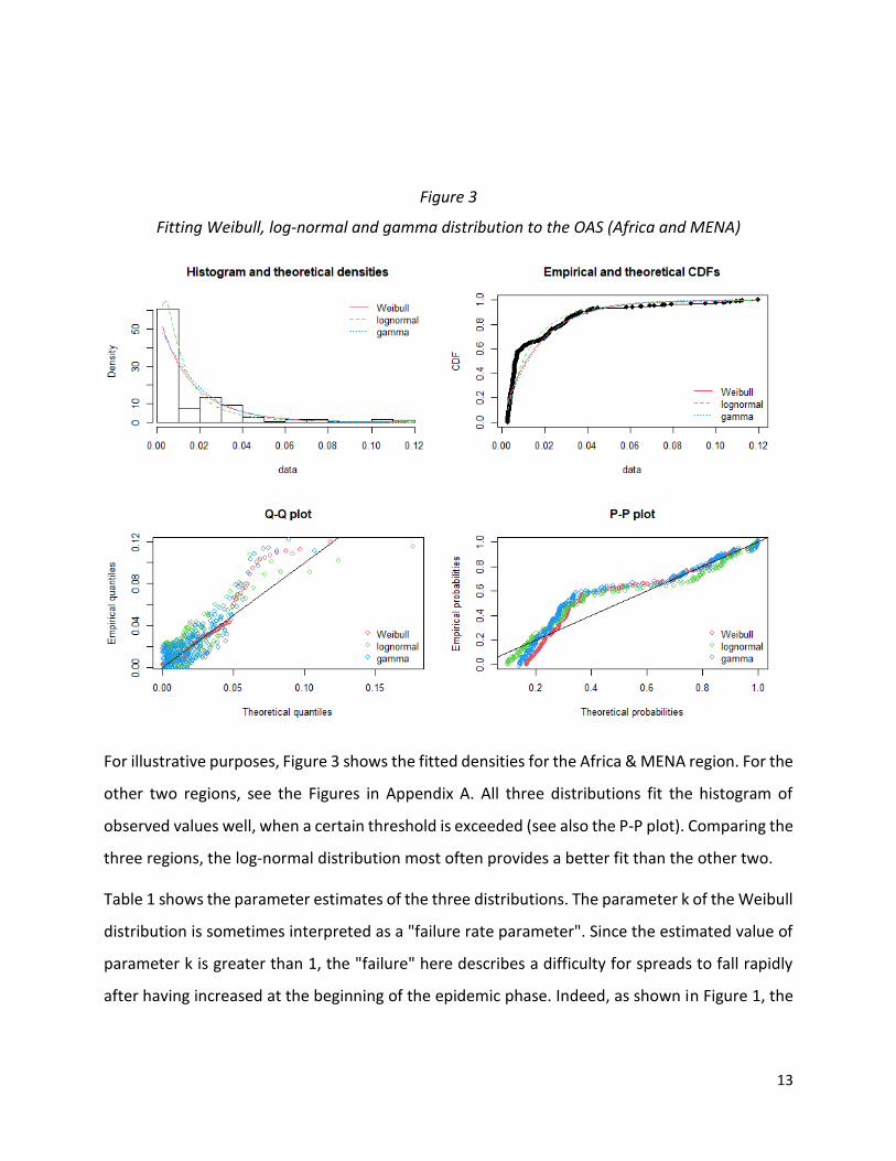
Figure 3

Fitting Weibull, log-normal and gamma distribution to the OAS (Africa and MENA)

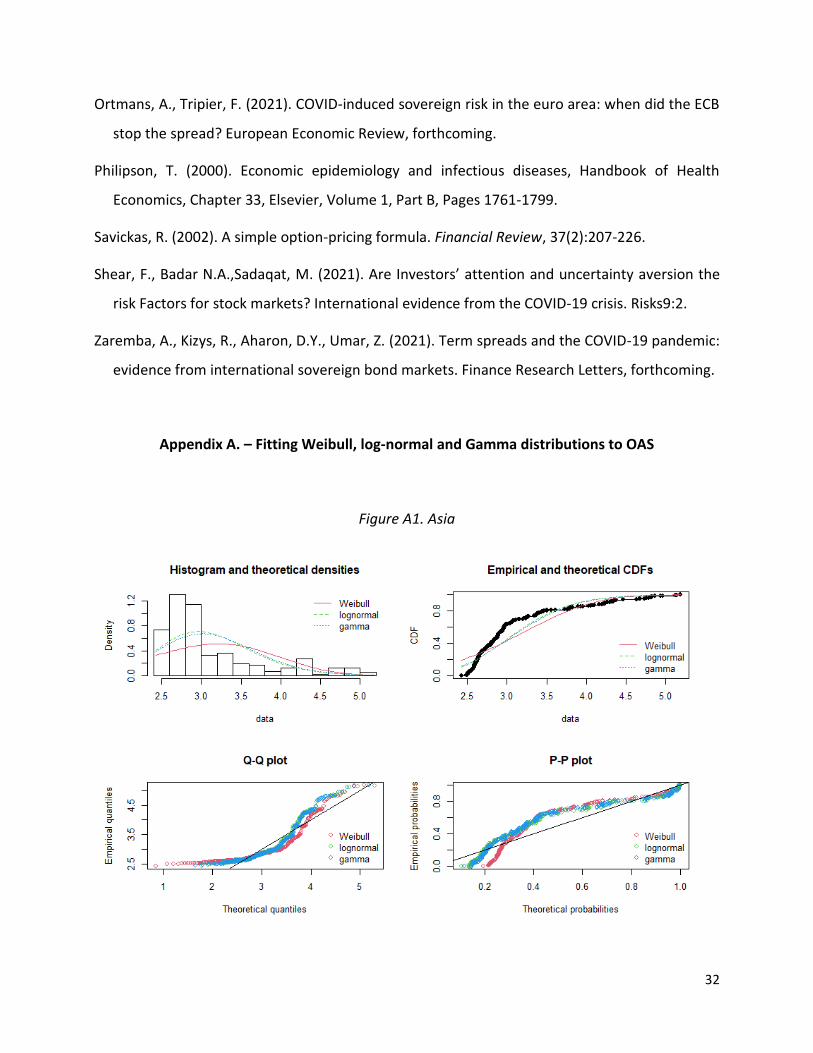
For illustrative purposes, Figure 3 shows the fitted densities for the Africa & MENA region. For the

other two regions, see the Figures in Appendix A. All three distributions fit the histogram of

observed values well, when a certain threshold is exceeded (see also the P-P plot). Comparing the

three regions, the log-normal distribution most often provides a better fit than the other two.

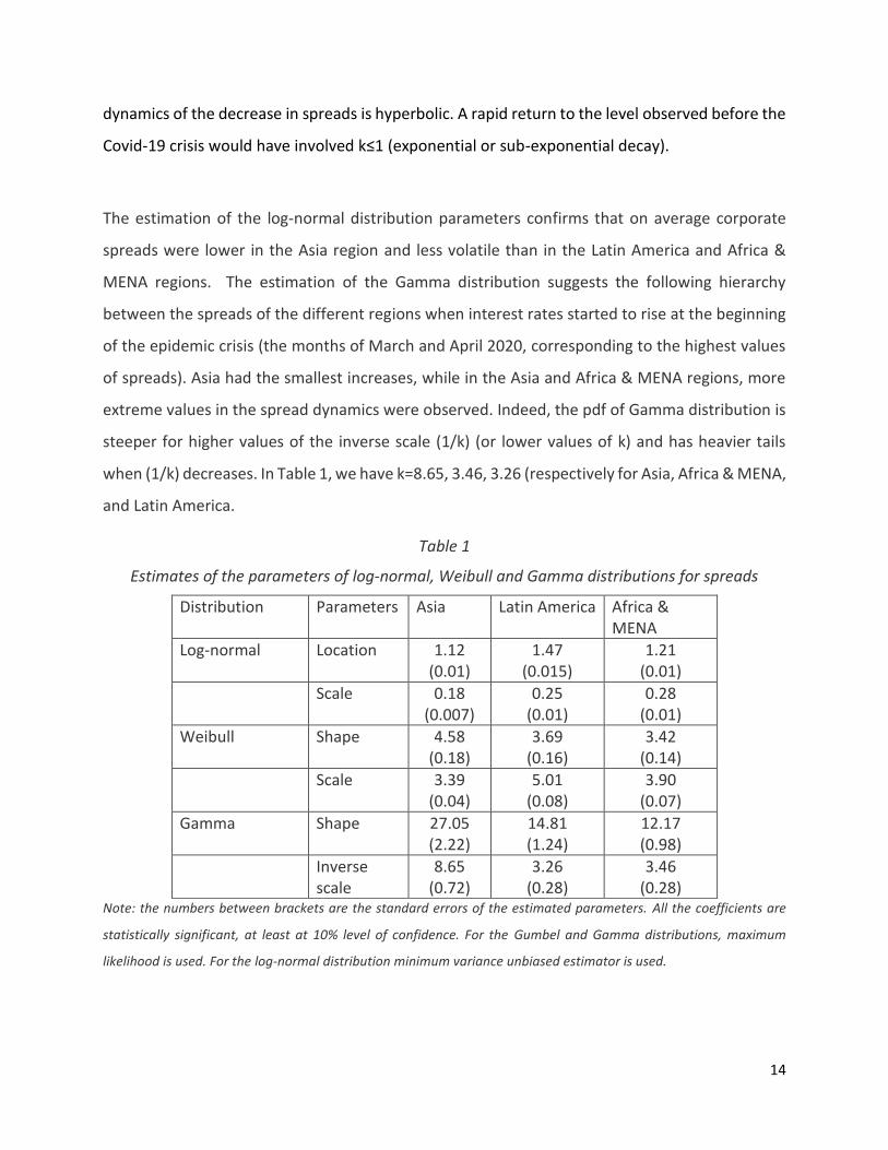
Table 1 shows the parameter estimates of the three distributions. The parameter k of the Weibull

distribution is sometimes interpreted as a "failure rate parameter". Since the estimated value of

parameter k is greater than 1, the "failure" here describes a difficulty for spreads to fall rapidly

after having increased at the beginning of the epidemic phase. Indeed, as shown in Figure 1, the

14

dynamics of the decrease in spreads is hyperbolic. A rapid return to the level observed before the

Covid-19 crisis would have involved k≤1 (exponential or sub-exponential decay).

The estimation of the log-normal distribution parameters confirms that on average corporate

spreads were lower in the Asia region and less volatile than in the Latin America and Africa &

MENA regions. The estimation of the Gamma distribution suggests the following hierarchy

between the spreads of the different regions when interest rates started to rise at the beginning

of the epidemic crisis (the months of March and April 2020, corresponding to the highest values

of spreads). Asia had the smallest increases, while in the Asia and Africa & MENA regions, more

extreme values in the spread dynamics were observed. Indeed, the pdf of Gamma distribution is

steeper for higher values of the inverse scale (1/k) (or lower values of k) and has heavier tails

when (1/k) decreases. In Table 1, we have k=8.65, 3.46, 3.26 (respectively for Asia, Africa & MENA,

and Latin America.

Table 1

Estimates of the parameters of log-normal, Weibull and Gamma distributions for spreads

Distribution Parameters Asia Latin America Africa & MENA

Log-normal Location 1.12 (0.01)

1.47 (0.015)

1.21 (0.01)

Scale 0.18 (0.007)

0.25 (0.01)

0.28 (0.01)

Weibull Shape 4.58 (0.18)

3.69 (0.16)

3.42 (0.14)

Scale 3.39 (0.04)

5.01 (0.08)

3.90 (0.07)

Gamma Shape 27.05 (2.22)

14.81 (1.24)

12.17 (0.98)

Inverse scale

8.65 (0.72)

3.26 (0.28)

3.46 (0.28)

Note: the numbers between brackets are the standard errors of the estimated parameters. All the coefficients are

statistically significant, at least at 10% level of confidence. For the Gumbel and Gamma distributions, maximum

likelihood is used. For the log-normal distribution minimum variance unbiased estimator is used.

15

3.2.- Epidemiological variables

Which indicator is the best basis for inference in epidemic data is still controversial in the epidemic

literature. It would be possible to estimate the reproduction rate by estimating contact interval

distribution, i.e. time from the onset of infectiousness to infectious contact (this approach is

typical to papers focusing on survival analysis of epidemics). The spreading behavior of Covid-19

is analyzed here using the following variables which are commonly used in the epidemiological

literature (data being collected on the Our world in data site (source: https://ourworldindata.org)

and Humanitarian Data Exchange (source: https://data.humdata.org/event/covid-19:

- Daily new confirmed cases vs cumulative cases,

- Confirmed deaths per million vs GDP per-capita,

- Reproduction rate,

- government response stringency index.

These data are taken for the three regions Asia, Latin and Central America and Africa & MENA.

As shown in Figure 4, the number of new cases versus cumulative cases has been steadily

decreasing. The same is true for the reproduction rate in the Africa & Mena and Latin America

regions (Figure 5). During the year 2020 and the first half of 2021, although all countries of the

world were affected, the epicenter of the pandemic was the industrialized countries of North

America and Europe. It is possible that the flattening epidemic curve in emerging countries has

led investors to underestimate the health risk, especially in Asia. On the other hand, the higher

level of spreads in Latin America could be explained by the fact that investors felt that the disease

was more serious in this region, because of the higher number of confirmed deaths versus GDP

per capita in the Latin American subcontinent (see Figure 6).

It is difficult, a priori, to say whether epidemiological factors have a high likelihood, or on the

contrary a low likelihood, of being correlated with spreads. Indeed, on the one hand, it is possible

that the dynamics of spreads were not correlated with those of epidemic factors. In the case of

Asia, this could be explained, for example, by the announced strategy of eradicating the virus in

this region (the so-called "zero-covid" strategy), while elsewhere in the world governments have

https://ourworldindata.org/

https://data.humdata.org/event/covid-19

16

opted instead for mitigation policies to simply reduce reproduction rates and contamination. For

the other two regions, one explanation would be that reproduction rates remained stable from

November 2021 and did not exceed the threshold of 1 (see Figure 5). Finally, a common

explanation for all continents could be that epidemic control measures were strong from the

beginning (school closures, travel restrictions, social distancing measures, border closures).

Figure 4

New cases versus cumulative cases

Source: Oxford Data base Our world in Data.

Figure 5

Covid-19 reproduction rate


00,020,040,060,08

0,10,120,140,160,18

Africa & Mena Asia Latin America

00,20,40,60,8

11,21,41,61,8


17

Figure 6

Confirmed deaths versus GDP per capita: Covid-19


Figure 7 shows the stringency index, which is an indicator of the severity of the restriction

measures implemented on a scale of 0 to 100 (100 being the highest level of severity). As can be

seen, governmental responses have been quick and strong (as of April 2021, the index is at least

60 in each of the regions studied).

On the other hand, it is possible to think that, on the contrary, epidemiological factors have

influenced the perception of health risk by investors and that this has been reflected in spreads.

For example, the previous figures show parallel developments between spreads and the

continuous decline in the new cases ratio. Similarly, the strict nature of the control measures may

have sent a signal to the markets, encouraging investors to keep emerging countries’ corporate

debts in their portfolios. Moreover, the direction of the correlation (positive or negative) is not

determined a priori. Indeed, it could be negative in the case of flight-to-safety behaviors (if the

crisis is perceived by investors as being more serious in other regions), or conversely positive.

As with the spreads, none of the four epidemiological variables has a Gaussian distribution. We

also estimate the parameters of Weibull, log-normal and Gamma distributions for these variables

and for each region. To avoid cluttering the paper with graphs, we do not report the resulting

00,00005

0,00010,00015

0,00020,00025

0,00030,00035

0,0004


18

figures (they are available on request from the authors). Instead, we report the estimated

parameters in Table 2.

Figure 7

Stringency index


If we first look at the news confirmed cases, we can see that the shape parameter of the Weibull

distribution is of the same order of magnitude in the three regions, which suggests a daily

propagation speed of the coronavirus at a similar rate during the first epidemic wave (period

under investigation). Indeed, the shape parameter captures here the spreading speed, i.e. the

occurrence of new cases within population. The scale parameter captures the spreading speed of

the disease since the first infection, i.e. how fast the new cases are progressing in relation to the

total days. Again, the values are identical from one region to another. The Gamma distribution

gives a different measure of the spread of the epidemic. Indeed, its parameters provide

information on the probability of remaining infectious. Lower values of k (shape parameter) and

larger values of θ - or equivalently lower values of 1/θ (inverse scale parameter) - in Equation (9c)

indicate a steeper increase in prevalence and a shorter duration epidemic. The data in Table 2

suggest that Asia had a lower prevalence of infection than the other two regions, but that the first

epidemic wave was longer. Epidemiological studies often find, at least for the first quarter of the

year 2020, that the number of new confirmed cases are distributed, in advanced countries and in

0102030405060708090

100


19

China, as a log-normal law. We find the same result here for emerging countries. Indeed, the

estimated parameters of the log-normal distribution are all statistically significant. This

distribution is interesting because it gives an idea of the decline of the epidemic after the peak of

the number of new cases. The more the tail of the distribution is spread to the right, the longer it

takes for the epidemic to die out. In Table 2, the parameter estimates suggest that the average

number of new cases was roughly the same in all regions during the first wave of the epidemic,

but that in the Asian region, infections faded more rapidly on average (shape parameter lower

than in Latin America and Africa & MENA).

The estimates for the confirmed deaths variable show a higher variance in the case of the Latin

America region (see the estimate of the scale parameter for the Weibull and log-normal

distributions, which is much higher than in the other two regions, and a smaller inverse scale for

the Gamma distribution). The estimates obtained for the reproduction rates do not suggest

significant differences in behavior between countries. The distributions for the stringency index

are interesting because the parameter values provide indications of the regenerative capacity of

public health policies, or in other words of "fatigue" in the implementation of policies aimed at

slowing the spread of the virus. In the case of Africa, it can be observed that the shape parameters

in the Weibull and Gamma distributions are much lower than those of the other two regions, and

that the scale parameter of the log-normal distribution is higher, suggesting greater variability in

the dynamics of the variable and the fact that the cumulative distribution function of this variable

is more "curved" than those of the Latin American and Asian regions.

4.- Which epidemiological variables are correlated with corporate OAS?

4.1.- Rank-correlation through a dynamic copula analysis

We previously observed that the distributions of both corporate OAS and epidemiological

variables are non- Gaussian and that they are heavy-tailed. We therefore consider tail

dependence in the data through a dynamic copula analysis. Our framework is the following.

20

Table 2

Estimates of the parameters of log-normal, Weibull and Gamma distributions for epidemiological variables

Asia Latin America Africa & MENA

New confirmed cases vs cumulative cases

Weibull Shape Scale

1.24 (0.04) 0.014 (0.0007)

1.07 (0.05) 0.017 (0.001)

0.95 (0.04) 0.01 (0.001)

Gamma Shape Inversed scale

1.95 (0.15) 144.5 (12.63)

1.26 (0.09) 76.04 (7.11)

1.05 (0.07) 60.070 (5.60)

Log-normal Location Shape

-45.8 (0.04) 0.67 (0.027)

-4.54 (0.05) 0.91 (0.038)

-4.60 (0.06) 0.98 (0.04)

Confirmed deaths versus GDP per capita

Weibull Shape Scale

1.58 (0.07) 2.16 (0.08)

2.17 (0.13) 27.27 (0.63)

1.62 (0.075) 4.32 (0.16)


2.05 (0.16) 1.05 (0.09)

4.14 (0.34) 0.17 (0.01)

1.94 (0.15) 0.49 (0.04)


0.40 (0.05) 0.85 (0.03)

3.07 (0.036) 0.603 (0.025)

1.08 (0.05) 0.94 (0.04)

Reproduction rate

Weibull Shape Scale

6.19 (0.24) 1.15 (0.01)

6.35 (0.25) 1.16 (0.01)

3.95 (0.14) 1.19 (0.02)


48.94 (4.03) 45.03 (3.73)

57.51 (4.89) 52.52 (4.48)

33.96 (2.78) 30.90 (2.55)


0.07 (0.008) 0.14 (0.005)

0.08 (0.007) 0.13 (0.005)

0.079 (0.009) 0.16 (0.006)

Government stringency index

Weibull Shape Scale

12.90 (0.55) 69.29 (0.33)

18.62 (0.87) 76.77 (0.26)

6.54 (0.28) 70.60 (0.67)


160.63 (13.27) 2.40 (0.199)

287.88 (24.53) 3.85 (0.33)

43.46 (3.57) 0.66 (0.054)


4.19 (0.004) 0.078 (0.003)

4.31 (0.003) 0.06 (0.002)

4.18 (0.008) 0.15 (0.006)

Note: the numbers between brackets are the standard errors of the estimated parameters. All the coefficients are

statistically significant, at least at 10% level of confidence. For the Gumbel and Gamma distributions, maximum

likelihood is used. For the log-normal distribution minimum variance unbiased estimator is used.

We estimate a Patton model to find the time-varying values of a rank correlation coefficient, i.e.

a bivariate Kendall’s 𝜏 dynamic process that account for lower and upper tail dependence:

21

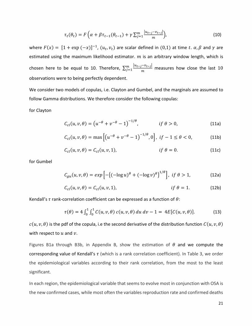
𝜏𝑡(𝜃𝑡) = 𝐹 (𝛼 + 𝛽𝜏𝑡−1(𝜃𝑡−1) + 𝛾 ∑|𝑢𝑡−𝑗−𝑣𝑡−𝑗|

𝑚

𝑚𝑗=1 ), (10)

where 𝐹(𝑥) = [1 + exp (−𝑥)]−1, (𝑢𝑡, 𝑣𝑡) are scalar defined in (0,1) at time 𝑡. 𝛼, 𝛽 and 𝛾 are

estimated using the maximum likelihood estimator. 𝑚 is an arbitrary window length, which is

chosen here to be equal to 10. Therefore, ∑|𝑢𝑡−𝑗−𝑣𝑡−𝑗|

𝑚

𝑚𝑗=1 measures how close the last 10

observations were to being perfectly dependent.

We consider two models of copulas, i.e. Clayton and Gumbel, and the marginals are assumed to

follow Gamma distributions. We therefore consider the following copulas:

for Clayton

𝐶𝑐𝑙(𝑢, 𝑣, 𝜃) = (𝑢−𝜃 + 𝑣−𝜃 − 1)−1/𝜃

, 𝑖𝑓 𝜃 > 0, (11a)

𝐶𝑐𝑙(𝑢, 𝑣, 𝜃) = max [(𝑢−𝜃 + 𝑣−𝜃 − 1)−1/𝜃

, 0] , 𝑖𝑓 − 1 ≤ 𝜃 < 0, (11b)

𝐶𝑐𝑙(𝑢, 𝑣, 𝜃) = 𝐶𝑐𝑙(𝑢, 𝑣, 1), 𝑖𝑓 𝜃 = 0. (11c)

for Gumbel

𝐶𝑔𝑢(𝑢, 𝑣, 𝜃) = 𝑒𝑥𝑝 [−{(−log 𝑢)𝜃 + (−log 𝑣)𝜃}1/𝜃

] , 𝑖𝑓 𝜃 > 1, (12a)

𝐶𝑐𝑙(𝑢, 𝑣, 𝜃) = 𝐶𝑐𝑙(𝑢, 𝑣, 1), 𝑖𝑓 𝜃 = 1. (12b)

Kendall’s 𝜏 rank-correlation coefficient can be expressed as a function of 𝜃:

𝜏(𝜃) = 4 ∫ ∫ 𝐶(𝑢, 𝑣, 𝜃) 𝑐(𝑢, 𝑣, 𝜃)1

0

1

0𝑑𝑢 𝑑𝑣 − 1 = 4𝐸[𝐶(𝑢, 𝑣, 𝜃)]. (13)

𝑐(𝑢, 𝑣, 𝜃) is the pdf of the copula, i.e the second derivative of the distribution function 𝐶(𝑢, 𝑣, 𝜃)

with respect to 𝑢 and 𝑣.

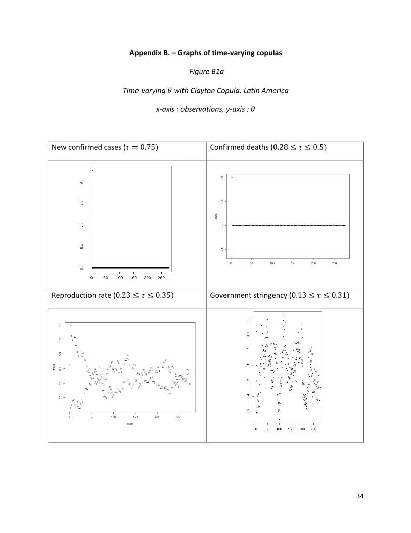
Figures B1a through B3b, in Appendix B, show the estimation of 𝜃 and we compute the

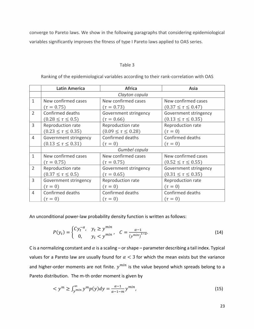
corresponding value of Kendall’s 𝜏 (which is a rank correlation coefficient). In Table 3, we order

the epidemiological variables according to their rank correlation, from the most to the least

significant.

In each region, the epidemiological variable that seems to evolve most in conjunction with OSA is

the new confirmed cases, while most often the variables reproduction rate and confirmed deaths

22

do not seem to be correlated with spreads. Government stringency has a higher correlation with

spreads in Africa than in the other two regions. In many cases, we observe a high variation of the

parameter 𝜃 across time. Such changes could be explained by the presence of nonlinear

relationships between corporate OAS and the epidemiological variables.

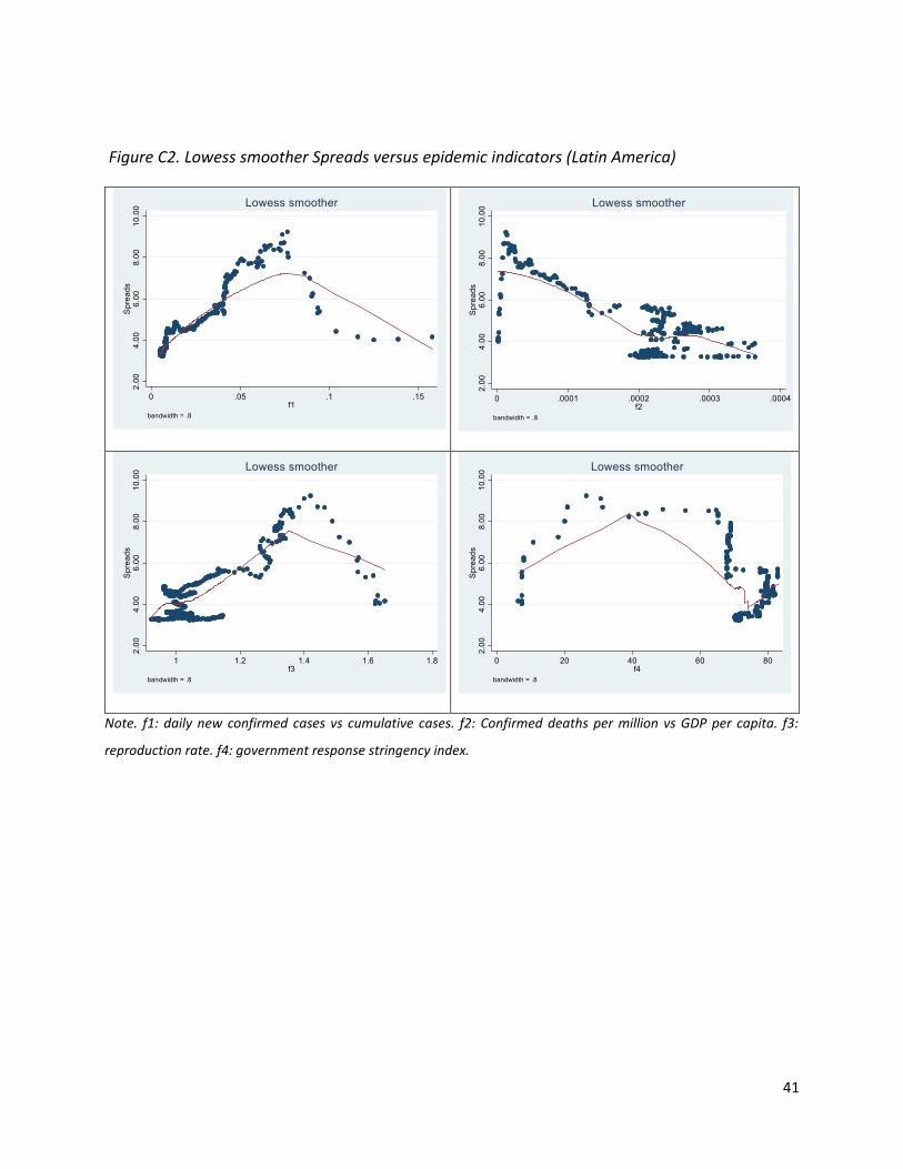
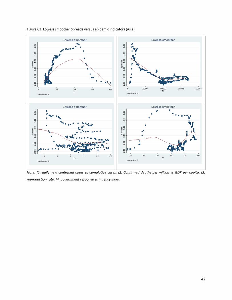
Figures C1 to C3, in Appendix C, suggest the existence of such nonlinear relationships. The curves

are obtained using a non-parametric LOWESS (locally weighted locally smoothing) adjustment.

For example, the relationship between OAS and new confirmed cases is represented by an

inverted U-shaped curve. If the ratio of new cases to cumulative cases is below a threshold,

spreads increase with the number of new cases. But beyond this threshold, we observe a

saturation effect, i.e. spreads continue to increase but at a lower rate. This phenomenon can be

explained by the kinetics of the propagation of Covid-19 which is identical to that of many viral

disease epidemics (S-Shaped). At the start of an epidemic wave, the disease spreads at an

exponential rate until the epidemic curve reaches an inflection point, at which the number of

newly infected persons increases more and more slowly until a plateau is reached. This plateau

generally marks the beginning of the epidemic's decline phase. The thresholds in the graphs

correspond to the periods of these inflection points on the Covid-A9 epidemic curves of the

different regions.

4.2.- Epidemiological variables are strong determinants of the right tail index of corporate

OAS distribution function

4.2.1.- Fitting Pareto laws

The graphs in Appendix C also show a difficulty in adjusting the curves to the points that are far

from the "center" of the graph, which can be called "outliers», and which correspond to the

highest spreads. These points probably follow different laws than the other points on the chart

(extreme value laws). We have seen, for example, that Weibull-type laws can be used to describe

our variables. The theory of extreme values teaches us that to study the behavior of values

beyond a certain threshold, we can find laws whose one of the parameters describes the

heaviness of the tail. Under certain conditions, the laws of excess above a certain threshold

23

converge to Pareto laws. We show in the following paragraphs that considering epidemiological

variables significantly improves the fitness of type I Pareto laws applied to OAS series.

Table 3

Ranking of the epidemiological variables according to their rank-correlation with OAS

Latin America Africa Asia

Clayton copula

1 New confirmed cases (𝜏 = 0.75)

New confirmed cases (𝜏 = 0.73)

New confirmed cases (0.37 ≤ 𝜏 ≤ 0.47)

2 Confirmed deaths (0.28 ≤ 𝜏 ≤ 0.5)

Government stringency (𝜏 = 0.66)

Government stringency (0.13 ≤ 𝜏 ≤ 0.35)

3 Reproduction rate (0.23 ≤ 𝜏 ≤ 0.35)

Reproduction rate (0.09 ≤ 𝜏 ≤ 0.28)

Reproduction rate (𝜏 = 0)

4 Government stringency (0.13 ≤ 𝜏 ≤ 0.31)

Confirmed deaths (𝜏 = 0)


Gumbel copula

1 New confirmed cases (𝜏 = 0.75)

New confirmed cases (𝜏 = 0.75)

New confirmed cases (0.52 ≤ 𝜏 ≤ 0.55)

2 Reproduction rate (0.37 ≤ 𝜏 ≤ 0.5)

Government stringency (𝜏 = 0.65)

Government stringency (0.31 ≤ 𝜏 ≤ 0.35)

3 Government stringency (𝜏 = 0)



4 Confirmed deaths (𝜏 = 0)



An unconditional power-law probability density function is written as follows:

𝑃(𝑦𝑡) = {𝐶𝑦𝑡

−𝛼, 𝑦𝑡 ≥ 𝑦𝑚𝑖𝑛

0, 𝑦𝑡 < 𝑦𝑚𝑖𝑛 , 𝐶 =

𝛼−1

(𝑦𝑚𝑖𝑛)1−𝛼. (14)

C is a normalizing constant and 𝛼 is a scaling – or shape – parameter describing a tail index. Typical

values for a Pareto law are usually found for 𝛼 < 3 for which the mean exists but the variance

and higher-order moments are not finite. 𝑦𝑚𝑖𝑛 is the value beyond which spreads belong to a

Pareto distribution. The m-th order moment is given by

< 𝑦𝑚 ≥ ∫ 𝑦𝑚𝑝(𝑦)𝑑𝑦 =𝛼−1

𝛼−1−𝑚𝑦𝑚𝑖𝑛∞

𝑦𝑚𝑖𝑛 , (15)

24

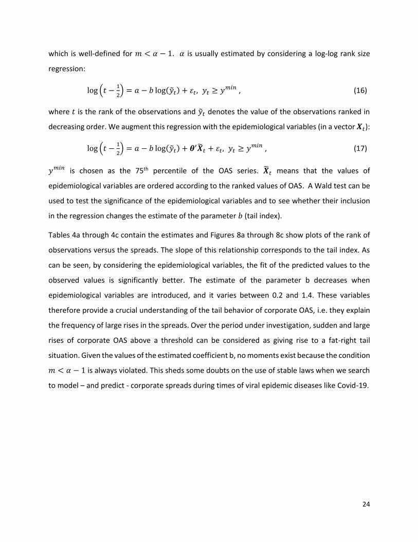
which is well-defined for 𝑚 < 𝛼 − 1. 𝛼 is usually estimated by considering a log-log rank size

regression:

log (𝑡 −1

2) = 𝑎 − 𝑏 log(�̃�𝑡) + 𝜀𝑡, 𝑦𝑡 ≥ 𝑦𝑚𝑖𝑛 , (16)

where 𝑡 is the rank of the observations and �̃�𝑡 denotes the value of the observations ranked in

decreasing order. We augment this regression with the epidemiological variables (in a vector 𝑿𝑡):

log (𝑡 −1

2) = 𝑎 − 𝑏 log(�̃�𝑡) + 𝜽′�̃�𝑡 + 𝜀𝑡, 𝑦𝑡 ≥ 𝑦𝑚𝑖𝑛 , (17)

𝑦𝑚𝑖𝑛 is chosen as the 75th percentile of the OAS series. �̃�𝑡 means that the values of

epidemiological variables are ordered according to the ranked values of OAS. A Wald test can be

used to test the significance of the epidemiological variables and to see whether their inclusion

in the regression changes the estimate of the parameter 𝑏 (tail index).

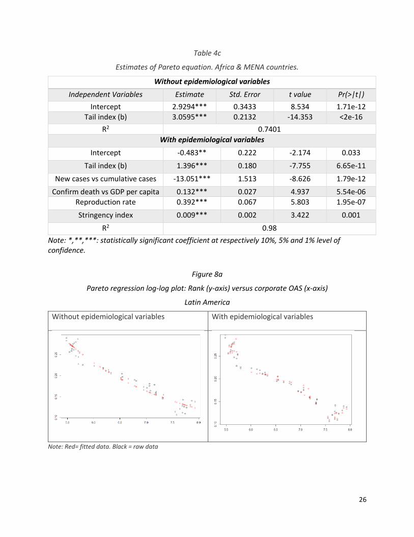
Tables 4a through 4c contain the estimates and Figures 8a through 8c show plots of the rank of

observations versus the spreads. The slope of this relationship corresponds to the tail index. As

can be seen, by considering the epidemiological variables, the fit of the predicted values to the

observed values is significantly better. The estimate of the parameter b decreases when

epidemiological variables are introduced, and it varies between 0.2 and 1.4. These variables

therefore provide a crucial understanding of the tail behavior of corporate OAS, i.e. they explain

the frequency of large rises in the spreads. Over the period under investigation, sudden and large

rises of corporate OAS above a threshold can be considered as giving rise to a fat-right tail

situation. Given the values of the estimated coefficient b, no moments exist because the condition

𝑚 < 𝛼 − 1 is always violated. This sheds some doubts on the use of stable laws when we search

to model – and predict - corporate spreads during times of viral epidemic diseases like Covid-19.

25

Table 4a

Estimates of Pareto equation. Latin American countries.

Without epidemiological variables

Independent Variables Estimate Std. Error t value Pr(>|t|)

Intercept 2.567*** 0.17072 15.04 <2e-16

Tail index (b) 2.25*** 0.09033 -24.91 <2e-16

R2 0.92

With epidemiologial variables

Intercept -0.687** 0.324 -2.117 0.039

Tail index (b) 0.244* 0.134 -1.819 0.075

New cases vs cumulative cases -5.788** 1.747 -3.313 0.002

Confirm death vs GDP per capita 0.015*** 0.001 8.953 1.00e-11

Reproduction rate -0.580*** 0.114 -5.087 6.26e-06

Stringency index 0.004*** 0.001 4.032 0.000

R2 0.99 Note: *,**,***: statistically significant coefficient at respectively 10%, 5% and 1% level of confidence

Table 4b

Estimates of Pareto equation. Asian countries.



Intercept 3,269*** 0,1907 17,15 <2e-16

Tail index (b) 3,691*** 0.1354 -27,26 <2e-16

R2 0,9128

With epidemiological variables

Intercept -0,232 0,3563 -0,652 0,5168

Tail index (b) 1,050*** 0,2441 -4,304 5,6e-05

New cases vs cumulative cases -19,691*** 2,045032 -9,629 2,9e-14

Confirm death vs GDP per capita 0,0758** 0,0368 2,059 0,0433

Reproduction rate 0,4632*** 0,1006 4,602 1,91e-05

Stringency index -0,0026 0,0030 -0,873 0,386

R2 0,9876 Note: *,**,***: statistically significant coefficient at respectively 10%, 5% and 1% level of confidence.

26

Table 4c

Estimates of Pareto equation. Africa & MENA countries.



Intercept 2.9294*** 0.3433 8.534 1.71e-12

Tail index (b) 3.0595*** 0.2132 -14.353 <2e-16

R2 0.7401

With epidemiological variables

Intercept -0.483** 0.222 -2.174 0.033

Tail index (b) 1.396*** 0.180 -7.755 6.65e-11

New cases vs cumulative cases -13.051*** 1.513 -8.626 1.79e-12

Confirm death vs GDP per capita 0.132*** 0.027 4.937 5.54e-06

Reproduction rate 0.392*** 0.067 5.803 1.95e-07

Stringency index 0.009*** 0.002 3.422 0.001

R2 0.98

Note: *,**,***: statistically significant coefficient at respectively 10%, 5% and 1% level of confidence.

Figure 8a

Pareto regression log-log plot: Rank (y-axis) versus corporate OAS (x-axis)

Latin America

Without epidemiological variables With epidemiological variables

Note: Red= fitted data. Black = raw data

27

Figure 8b


Africa & MENA



Figure 8c


Asia



28

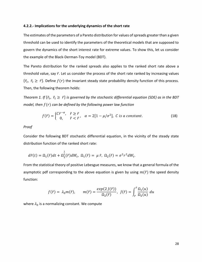
4.2.2.- Implications for the underlying dynamics of the short rate

The estimates of the parameters of a Pareto distribution for values of spreads greater than a given

threshold can be used to identify the parameters of the theoretical models that are supposed to

govern the dynamics of the short interest rate for extreme values. To show this, let us consider

the example of the Black-Derman-Toy model (BDT).

The Pareto distribution for the ranked spreads also applies to the ranked short rate above a

threshold value, say �̅�. Let us consider the process of the short rate ranked by increasing values

{�̃�𝑡, �̃�𝑡 ≥ �̅�}. Define 𝑓(𝑟) the invariant steady state probability density function of this process.

Then, the following theorem holds:

Theorem 1. If {�̃�𝑡, �̃�𝑡 ≥ �̅�} is governed by the stochastic differential equation (SDE) as in the BDT

model, then 𝑓(𝑟) can be defined by the following power law function

𝑓(�̃�) = {𝐶�̃�−𝛼, �̃� ≥ �̅�

0, �̃� < �̅� , 𝛼 = 2[1 − 𝜇/𝜎2], 𝐶 𝑖𝑠 𝑎 𝑐𝑜𝑛𝑠𝑡𝑎𝑛𝑡. (18)

Proof

Consider the following BDT stochastic differential equation, in the vicinity of the steady state

distribution function of the ranked short rate:

𝑑�̃�(𝑡) = Ω1(�̃�)𝑑𝑡 + Ω2

1

2 (�̃�)𝑑𝑊𝑡, Ω1(�̃�) = 𝜇 �̃�, Ω2(�̃�) = 𝜎2𝑟2𝑑𝑊𝑡.

From the statistical theory of positive Lebesgue measures, we know that a general formula of the

asymptotic pdf corresponding to the above equation is given by using 𝑚(�̃�) the speed density

function:

𝑓(�̃�) = 𝜆0𝑚(�̃�), 𝑚(�̃�) =𝑒𝑥𝑝(2 𝐽(�̃�))

Ω2(�̃�), 𝐽(�̃�) = ∫

Ω1(𝑢)

Ω2(𝑢)

�̃�

�̅�

𝑑𝑢

where 𝜆0 is a normalizing constant. We compute

29

𝜆0𝑚(�̃�) =𝜆0

𝜎2𝑟2𝑒𝑥𝑝 [2 ∫

𝜇 𝑢

𝜎2 𝑢2

�̃�

�̅�

𝑑𝑢]

=𝜆0

𝜎2𝑟2𝑒𝑥𝑝 [2

𝜇

𝜎2 ln (

�̃�

�̅�)]

=𝜆0

𝜎2(�̅�)−2 (

�̃�

�̅�)

−2(1−𝜇

𝜎2)

Finally, we have

𝑓(�̃�) = 𝐶(�̃�)−𝛼, 𝐶 =𝜆0

𝜎2(�̅�)𝛼−2, 𝛼 = 2[1 − 𝜇/𝜎2], �̃� ≥ �̅�.

This corresponds to a power law pdf, like in Equation 14, with 𝛼 = 2[1 − 𝜇/𝜎2]. We then

calculate the normalizing constant 𝜆0 such that ∫ 𝑓(𝑢)𝑑𝑢 = 1.+∞

�̅� We obtain 𝜆0 = −�̅�(2𝜇 − 𝜎2).

◼

Once 𝛼 and 𝐶 are estimated as in the previous section, their estimates can serve as identification

conditions to find the threshold value �̅� above which the process {�̃�𝑡, �̃�𝑡 ≥ �̅�} converges to a

steady state distribution described by a power-law function. Define �̂� and �̂� as the estimate of

the tail index coefficient and intercept in the log-log rank regression (Equations 16 or 17). Then,

we define the following system of two equations:

{�̂� = 2[1 − 𝜇/𝜎2],

�̂� =−�̅�(2𝜇−𝜎2)

𝜎2(�̅�)�̂�−2.

(19)

There is an infinite number of values for 𝜇 and 𝜎2 that satisfy this sytem, but only one value for �̅�

which is obtained by eliminating either 𝜇 or 𝜎2 when solving the system by substitution.

5.- Conclusion

The results of our paper show that epidemiological variables related to the first wave of the Covid-

19 crisis from March 2020 to April 2021 had an influence on corporate OAS in emerging countries.

Thus, information about the spread of the epidemic became part of the informational set of

investors in emerging market corporate debt. Variables such as the number of new cases,

reproduction rates, mortality rates or containment policies may explain why spreads become

30

higher during the acute phases of the crisis, but more importantly why their future evolution is

impossible to predict. This is highlighted by the non-existence of moments for the Pareto law that

we have estimated.

In prioritizing the variables, the one that changes most in conjunction with RSA is the number of

new cases, and the variable that appears to change most independently of the spreads is the

mortality rate. Our statistical analysis opposes the idea that investors are primarily sensitive to

the fundamental variables of companies in deciding to buy their debt. Global variables, notably

epidemiological ones, influence their decisions. Our study has at least one implication. While the

epidemic is not yet over, the succession of several epidemic waves in the future could make the

evolution of spreads unpredictable.

References

Ahir, H., Bloom, N., Furceri, D. (2018). World uncertainty index, Stanford and IMF, Available at

SSRN: https://ssrn.com/abstract=3275033 or http://dx.doi.org/10.2139/ssrn.3275033

Alentorn, A. and Markose, S. (2011). The generalized extreme value distribution, implied tail

index, and option pricing. The Journal of Derivatives, 18(31), 35-60.

Aramonte, S., Avalos, F. (2020). Corporate credit markets after the initial pandemic shock. BIS

Bulletin, n°26.

Baker, S. R., Bloom, N. Davis, S.J. and Terry, S.J. (2020). COVID-induced economic uncertainty.

NBER Working Paper No. w26983.

Bahij, M., Nafidi, A., Achchab, B., Gama, S., and Matos, J. (2016). A stochastic diffusion process

based on the two-parameters Weibull density function. International Journal of Mathematical,

Computational, Physical, Electrical and Computer Engineering, 10(6):254-259.

Bordo, M.D., Duca, J.V. (2020). How new Fed corporate bond programs dampened the financial

accelerator in the COVID-19 recession. Federal Reserve Banks of Dallas Working Paper 2029.

Daehler, T.B., Aizenman, J., Jinjarak, Y. (2021). Emerging market sovereign CDS spreads during

COVID-19: Economics versus epidemiology news. Economic Modelling, 100, forthcoming.

https://ssrn.com/abstract=3275033

https://dx.doi.org/10.2139/ssrn.3275033

31

Eberlein, E., Madan, D., Pistorius, M., Yor, M. (2013). A simple stochastic rate model for rate equity

hybrid products. Applied Mathematical Finance 20:461–488.

Ebsim, M., Faria-e-Castro, M., Kozlowski, J. (2021). Corporate borrowing, investment, and credit

policies during large crises. Federal Reserve Bank of Saint Louis, Economic Research Working

Paper 2020-035B.

Feyen, E., Dancausa, F., Gurhy, B., Nie, O. (2020). COVID-19 and EMDE corporate balance sheet

vulnerabilities: a simple stress-test approach. Policy Research Working Paper No. 9324. World

Bank, Washington DC.

Gilchrist, S., Wei, B., Yue, V.Z., Zakrajšek, E. (2020). "The Fed takes on corporate credit risk: an

analysis of the efficacy of the SMCCF," NBER Working Papers 27809, National Bureau of

Economic Research.

Gubareva, M. (2021). Covid-19 and high-yield emerging market bonds: insights for liquidity risk

management. Risk Management, April.

Haroon, O. and S.A.R. Rizvi (2020), Flatten the curve and stock market liquidity. An inquiry into

emerging market. Emerging Markets Finance and Trade, 56(10):2151-2161.

James, L. F., M ̈uller, G., Zhang, Z. (2017). Stochastic volatility models based on OU-gamma time

change: Theory and estimation. Journal of Business & Economic Statistics 36, 1–13.

Kargar, M., Lester, B., Lindsay, D., Liu, S., Weill, P.-O., Zúñiga, D. (2021). Corporate Bond Liquidity

during the COVID-19 Crisis, The Review of Financial Studies, forthcoming.

Kawai, R., Takeuchi, A. (2010). Sensitivity analysis for averaged asset price dynamics with gamma

processes. Statistics & Probability Letters 80 (1), 42–49.

Liang, J.N. (2020). Corporate bond markets dysfunction during the COVID-19 and lessons from the

Fed’s response. Hutchins Center Working Paper # 69.

Narayan, P. K., and Phan. , D. H. B. (2020). Country responses and the reaction of the stock market

to COVID-19—A preliminary exposition. Emerging Markets Finance and Trade. 56 (10):2138–

2150.

https://ideas.repec.org/p/nbr/nberwo/27809.html

https://ideas.repec.org/p/nbr/nberwo/27809.html

https://ideas.repec.org/s/nbr/nberwo.html

32

Ortmans, A., Tripier, F. (2021). COVID-induced sovereign risk in the euro area: when did the ECB

stop the spread? European Economic Review, forthcoming.

Philipson, T. (2000). Economic epidemiology and infectious diseases, Handbook of Health

Economics, Chapter 33, Elsevier, Volume 1, Part B, Pages 1761-1799.

Savickas, R. (2002). A simple option-pricing formula. Financial Review, 37(2):207-226.

Shear, F., Badar N.A.,Sadaqat, M. (2021). Are Investors’ attention and uncertainty aversion the

risk Factors for stock markets? International evidence from the COVID-19 crisis. Risks9:2.

Zaremba, A., Kizys, R., Aharon, D.Y., Umar, Z. (2021). Term spreads and the COVID-19 pandemic:

evidence from international sovereign bond markets. Finance Research Letters, forthcoming.

Appendix A. – Fitting Weibull, log-normal and Gamma distributions to OAS

Figure A1. Asia

33

Figure A2. Latin America

34

Appendix B. – Graphs of time-varying copulas

Figure B1a

Time-varying 𝜃 with Clayton Copula: Latin America

x-axis : observations, y-axis : 𝜃

New confirmed cases (𝜏 = 0.75) Confirmed deaths (0.28 ≤ 𝜏 ≤ 0.5)

Reproduction rate (0.23 ≤ 𝜏 ≤ 0.35) Government stringency (0.13 ≤ 𝜏 ≤ 0.31)

35

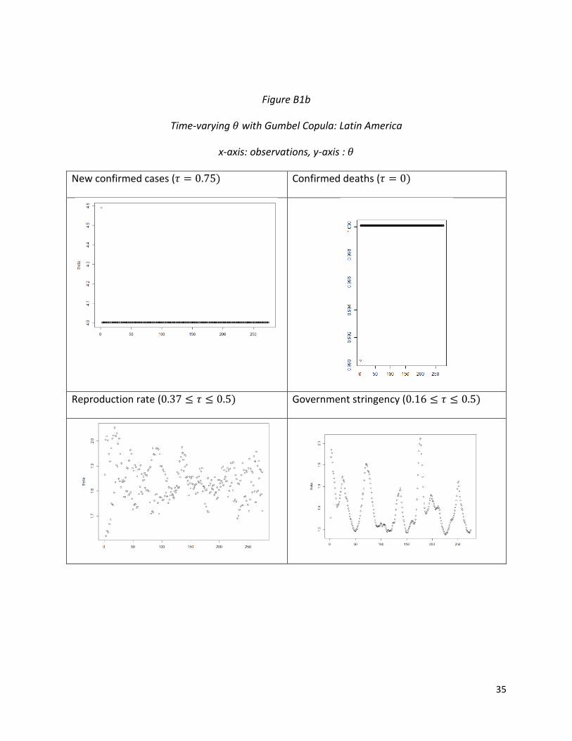
Figure B1b

Time-varying 𝜃 with Gumbel Copula: Latin America

x-axis: observations, y-axis : 𝜃

New confirmed cases (𝜏 = 0.75) Confirmed deaths (𝜏 = 0)

Reproduction rate (0.37 ≤ 𝜏 ≤ 0.5) Government stringency (0.16 ≤ 𝜏 ≤ 0.5)

36

Figure B2a

Time-varying 𝜃 with Clayton Copula: Africa & MENA


New confirmed cases (𝜏 = 0.73) Confirmed deaths (average 𝜏 = 0)

Reproduction rate (0.09 ≤ 𝜏 ≤ 0.28) Government stringency (𝜏 = 0.66)

37

Figure B2b

Time-varying 𝜃 with Gumbel Copula: Africa & MENA


New confirmed cases (𝜏 = 0.75) Confirmed deaths (𝜏 = 0)

Reproduction rate (𝜏 = 0) Government stringency (𝜏 = 0.65)

38

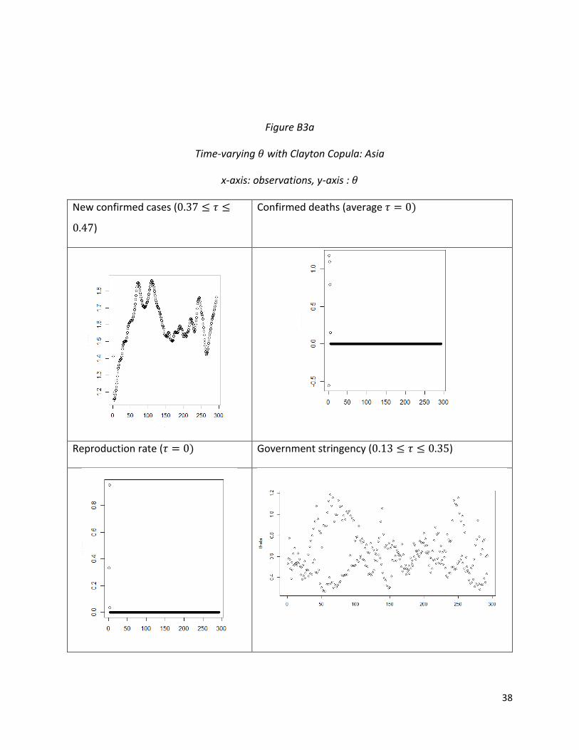
Figure B3a

Time-varying 𝜃 with Clayton Copula: Asia


New confirmed cases (0.37 ≤ 𝜏 ≤

0.47)

Confirmed deaths (average 𝜏 = 0)

Reproduction rate (𝜏 = 0) Government stringency (0.13 ≤ 𝜏 ≤ 0.35)

39

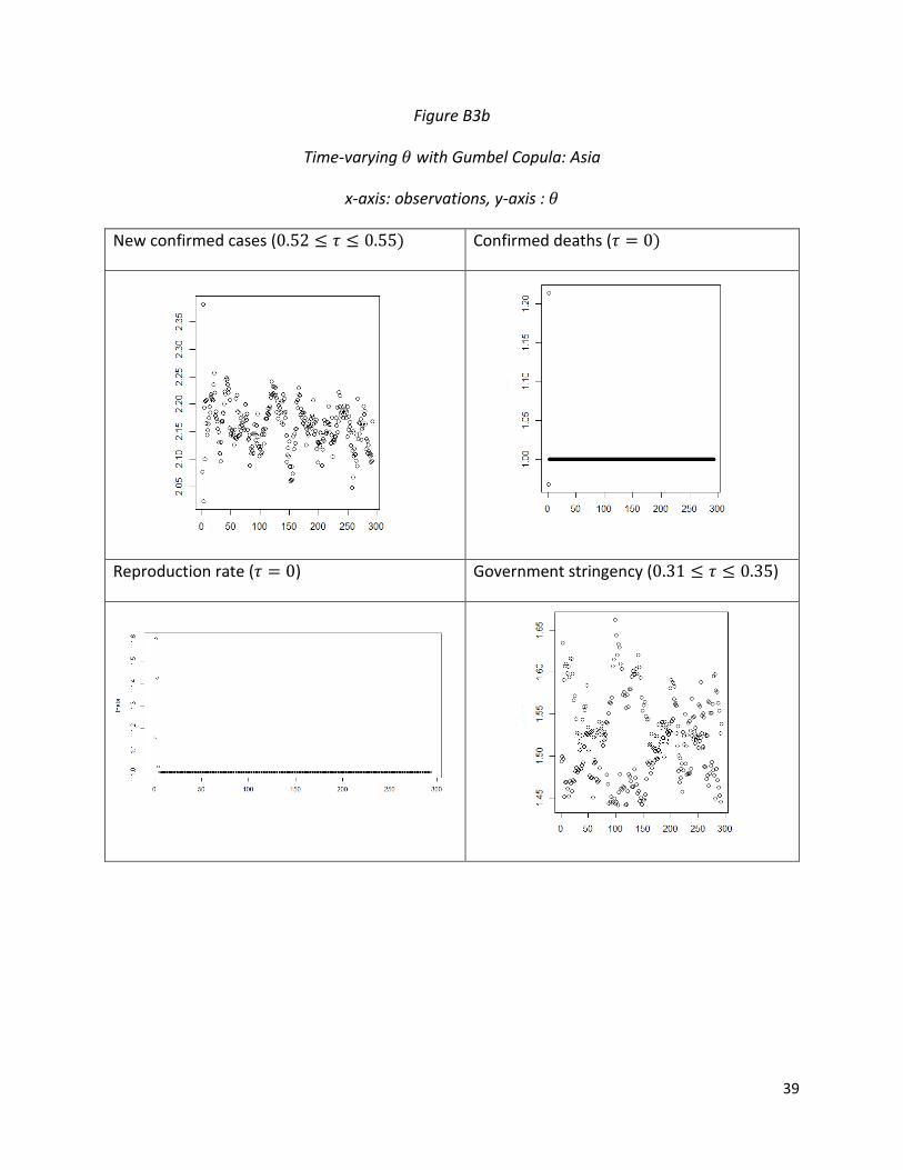
Figure B3b

Time-varying 𝜃 with Gumbel Copula: Asia


New confirmed cases (0.52 ≤ 𝜏 ≤ 0.55) Confirmed deaths (𝜏 = 0)

Reproduction rate (𝜏 = 0) Government stringency (0.31 ≤ 𝜏 ≤ 0.35)

40

Appendix C. – Evidence of nonlinear relationships

Figure C1. Lowess smoother Spreads versus epidemic indicators (Africa & MENA)

Note. f1: daily new confirmed cases vs cumulative cases. f2: Confirmed deaths per million vs GDP per capita. f3:

reproduction rate. f4: government response stringency index.

41

Figure C2. Lowess smoother Spreads versus epidemic indicators (Latin America)



42

Figure C3. Lowess smoother Spreads versus epidemic indicators (Asia)

