Embed Size (px)
Citation preview

Imaging Through Atmospheric Turbulence inRemote Sensing
PSF Estimation and Deblurring for Hyperspectral Imaging
Bob Plemmons
WFU
Sanya China, Jan. 2015
Starry Night - Vincent van Gogh
Bob Plemmons (WFU) Spectral Imaging Through Turbulence Sanya China, Jan. 2015 1 / 52

Outline
Overview of Optical Imaging in Remote SensingOur Recent Projects(Imaging Through) Turbulence: da Vinci, Galileo,Komolgorov, Von KarmanHyperspectral Imaging (HSI)Estimating HSI PSFs for Atmospheric TurbulenceJoint Sparse Deblurring and Feature ExtractionIf time: Compressive Snapshot Spectral -Polarimetric Imaging
Bob Plemmons (WFU) Spectral Imaging Through Turbulence Sanya China, Jan. 2015 2 / 52

References Related to Presentation
Zhao, Wang, Huang, Ng, Ple. “Deblurring and sparse unmixing forhyperspectral images”. IEEE, Geoscience and Remote Sensing, 2013.
Berisha, Nagy and Ple. “Estmation of Wavelength Dependent PSFs forDeblurring Hyperspectral Images,”, in revision, 2015.
Berisha, Nagy and Ple. “Deblurring and Sparse Unmixing ofHyperspectral Images using Multiple PSFs,”, in revision, 2015.
Ple., Prasad, Berisha, Pauca, “Compressive Spectral andSpectro-Polarimetric Images Taken Trough Atmospheric Turbulence,”preprint in progress.
First 3 available at: http://users.wfu.edu/plemmons/
Bob Plemmons (WFU) Spectral Imaging Through Turbulence Sanya China, Jan. 2015 3 / 52

Optical Remote Sensing
2015 has been proclaimed the International Year of Light andLight-Related Technologies by UNESCO.
Optical sensors form images of objects or scenes by detectingtheir solar or laser reflectance.
Hyperspectral (2D spatial & 1D wavelength) andLiDAR (2D spatial & 1D range) Imaging
Hyperspectral imaging (HSI) collects information across the visibleand IR spectrum for interrogating scenes.LiDAR measures distance by illuminating targets with a scanninglaser and analyzing the reflected light. Laser wavelengths vary tosuit the target: 10 µm to UV. Very short.Fused HSI and LiDAR for enhanced analysis. Combined laserranging & object material identification.
Spectro-Polarimetric imaging (3D hyperspectral & 1Dpolarization). Data is a 4D tensor. Polarization identifies objectshape, metallic surfaces.
Bob Plemmons (WFU) Spectral Imaging Through Turbulence Sanya China, Jan. 2015 4 / 52

Bob Plemmons (WFU) Spectral Imaging Through Turbulence Sanya China, Jan. 2015 5 / 52

NGA HSI/LiDAR Project
Implicit Geometry Framework (IGF) using level set methods forLiDAR data representation and compression. “A Novel Approachto Environment Reconstruction In LIDAR and HSI Datasets.”Randomized matrix and tensor factorization for HSI compression.Low-rank matrix approximations, e.g., approx. tSVD of HSItensor, then fusion of components with LiDAR data.Clustering and classification of fused data, andinformation-theoretic results, detecting objects in shadows, etc.New project: Information-theoretic Fusion and Analysis of HSI,LiDAR and Polarimetric Data.
NGA Campus
Bob Plemmons (WFU) Spectral Imaging Through Turbulence Sanya China, Jan. 2015 6 / 52

Bob Plemmons (WFU) Spectral Imaging Through Turbulence Sanya China, Jan. 2015 7 / 52

Turbulence
Image contains sketch by Leonardo da Vinci, along with a remarkablymodern description: “ the smallest eddies are almost numberless, andlarge things are rotated only by large eddies and not by small ones.”Called phenomena “turbolenza”, leading to modern word turbulence.
Bob Plemmons (WFU) Spectral Imaging Through Turbulence Sanya China, Jan. 2015 8 / 52

Atmospheric Turbulence
Later, Galileo, 1564-1642, knew effects of atmospheric turbulence ontelescopes. Modern mathematical models developed by:
(a) Th. von Karman, 1881-1963 (b) Andrey Kolmogorov, 1903-1987
Figure 1: Example of atmospheric turbulence blurring for video imaging at adistance of 1 km.
Bob Plemmons (WFU) Spectral Imaging Through Turbulence Sanya China, Jan. 2015 9 / 52

Atmospheric Turbulence Effects on Optical Images
Earth’s atmosphere is turbulent and variations in the index ofrefraction cause the plane optical wavefront from distantobjects to be distorted. Caused by variation of air temperaturein eddies and air currents. Arriving light wavefront is crumpled.In astronomy, or space situational awareness, resolution of allground-based telescopes is severely limited by effects ofatmospheric turbulence. At best sites, the resolution of a 2.5mtelescope is degraded by at least a factor of five.Can cause blurring in ground-level (horizontal) imaging. Forhorizontal image beam paths, ground based turbulencetypically has a highly non-Kolmogorov power spectraldensity (PSD), and both phase and amplitude perturbations(scintillations) must be included in PSF model.
Bob Plemmons (WFU) Spectral Imaging Through Turbulence Sanya China, Jan. 2015 10 / 52
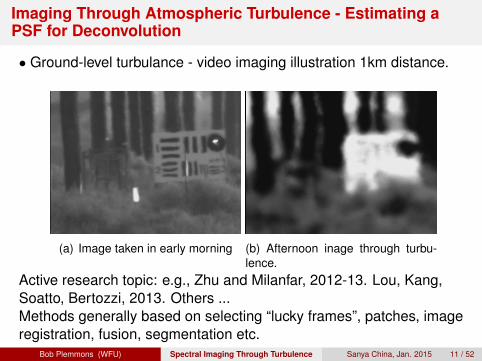
Imaging Through Atmospheric Turbulence - Estimating aPSF for Deconvolution
• Ground-level turbulance - video imaging illustration 1km distance.
(a) Image taken in early morning (b) Afternoon inage through turbu-lence.
Active research topic: e.g., Zhu and Milanfar, 2012-13. Lou, Kang,Soatto, Bertozzi, 2013. Others ...Methods generally based on selecting “lucky frames”, patches, imageregistration, fusion, segmentation etc.
Bob Plemmons (WFU) Spectral Imaging Through Turbulence Sanya China, Jan. 2015 11 / 52

Imaging Through Atmospheric Turbulence - Estimating aPSF, or PSFs, for Deconvolution
• Astronomical imaging, looking up
Nagy, Jefferies and Chu 2010, 2014 . R. Chan, X. Yuan and W. Zhang2012, 2013. Berisha, Nagy, Plemmons 2015. Others ...Methods based on wavefront sensing (Shack-Hartman), gradient &phase estimation leading to a PSF, or turbulence modeling.
Bob Plemmons (WFU) Spectral Imaging Through Turbulence Sanya China, Jan. 2015 12 / 52
Hyperpectral Imaging (HSI)
• Spectral imagers capture a 3D datacube (tensor)containing:
2D spatial information: x-y1D spectral information at each spatial location: λ
• Pixel intensity varies with wavelength bands -provides a spectral trace of intensity values.
• Generates a spatial map of spectral variation.
• Challenging to remove atmospheric turbulence blurfrom HSI.
Bob Plemmons (WFU) Spectral Imaging Through Turbulence Sanya China, Jan. 2015 13 / 52

Spectral (beyond RGB) Imaging at Wavelengths λ
Figure 2: λ generally ranges between 400 and 2500 nanometers.
Bob Plemmons (WFU) Spectral Imaging Through Turbulence Sanya China, Jan. 2015 14 / 52

Structure of HSI Data
Bob Plemmons (WFU) Spectral Imaging Through Turbulence Sanya China, Jan. 2015 15 / 52

Extract Spectral Signatures (Traces) from HSI toIdentify Materials
Figure 3: Illustration High Resolution - Each pixel represents a vector
Bob Plemmons (WFU) Spectral Imaging Through Turbulence Sanya China, Jan. 2015 16 / 52

Some Applications of HSI
Detect and identifymilitarily importantobjects at a distance.
Identification of plantspecies.Food processing.Mineral resourceassessments.Medicine.Enable space objectidentification & analysisfrom the ground.
http://www.globalsecurity.org/intell/library/imint/hyper.htm
Bob Plemmons (WFU) Spectral Imaging Through Turbulence Sanya China, Jan. 2015 17 / 52

Some Applications of HSI
Detect and identifymilitarily importantobjects at a distance.
Identification of plantspecies.
Food processing.Mineral resourceassessments.Medicine.Enable space objectidentification & analysisfrom the ground.
www.fujitsu.com/global/about/resources/news/press-releases/2011/0715-01.html
Bob Plemmons (WFU) Spectral Imaging Through Turbulence Sanya China, Jan. 2015 17 / 52

Some Applications of HSI
Detect and identifymilitarily importantobjects at a distance.Identification of plantspecies.
Food processing.
Mineral resourceassessments.Medicine.Enable space objectidentification & analysisfrom the ground.
http://photonics.com/Article.aspx?AID=51023
Bob Plemmons (WFU) Spectral Imaging Through Turbulence Sanya China, Jan. 2015 17 / 52

Some Applications of HSI
Detect and identifymilitarily importantobjects at a distance.Identification of plantspecies.Food processing.
Mineral resourceassessments.
Medicine.Enable space objectidentification & analysisfrom the ground.
www.usgs.gov/blogs/features/usgs_science_pick/hyperspectral-hypercoverage/
Bob Plemmons (WFU) Spectral Imaging Through Turbulence Sanya China, Jan. 2015 17 / 52

Some Applications of HSI
Detect and identifymilitarily importantobjects at a distance.Identification of plantspecies.Food processing.Mineral resourceassessments.
Medicine.
Enable space objectidentification & analysisfrom the ground.
http://mix.msfc.nasa.gov/abstracts.php?p=2700
Bob Plemmons (WFU) Spectral Imaging Through Turbulence Sanya China, Jan. 2015 17 / 52

Some Applications of HSI
Detect and identifymilitarily importantobjects at a distance.Identification of plantspecies.Food processing.Mineral resourceassessments.Medicine.
Enable space objectidentification & analysisfrom the ground.
http://www.afspc.af.mil/news1/story.asp?id=123369595
http://www.wpafb.af.mil/news/story.asp?id=123331461
Bob Plemmons (WFU) Spectral Imaging Through Turbulence Sanya China, Jan. 2015 17 / 52

Elementary Optics - HSI Resolution Revolution (PhysicsToday, Dec. 2014)
German physicist Ernst Abbe realized the resolution of animaging instrument is constrained by the wavelength of lightused, and the aperture of its optics.Resolution (detail an image holds) of a given telescope isproportional to the size of its aperture, and inverselyproportional to the wavelength of the light being observed:Res ≈ d/λ. - opposite to the effect of atmospheric turbulence.Resolution also affected by blur & noise.Our purpose: estimate wavelength dependent PSFs for HSI.
Bob Plemmons (WFU) Spectral Imaging Through Turbulence Sanya China, Jan. 2015 18 / 52

Hyperspectral Imaging (HSI) - Atmospheric PSFs
The image acquired at wavelength λ can be represented as
gλ(x , y) = hλ(x , y ;φ) ∗ f (x , y , λ) + ελ(x , y),
where the blurring kernel, with diffractive scaling included, is
hλ(x , y ;φ) =
(λ0
λ
)2
h0
(λ0
λx ,λ0
λy ;φ
),
with λ0 = reference baseline wavelength, and
h0(x , y ;φ) =∣∣∣F−1
(peiφ
)∣∣∣2 ,and where the wavefront phase φ = 2π
λ ×OPD.
• OPD is the optical path difference function, i.e. the optical phaseshift in passage through turbulent atmosphere. OPD is essentially thesame for each HSI wavelength, but the wavefront phase is not.
Bob Plemmons (WFU) Spectral Imaging Through Turbulence Sanya China, Jan. 2015 19 / 52

Tracking the PSFs as a Function of Wavelength
• Model phase function using the von Karman phase spectrum,
P(κx , κy ) =√.023(D/r0)5/3(κ2
0 + κ2x + κ2
y )−11/6,
where r0: Fried parameter, D: telescope aperture diameter, κ0:low-freq cutoff.
• φ =√
P(κx , κy ) W (κx , κy ), where W is a zero-mean, unit-variance,white Gaussian noise array. Set D/r0 = 10.
• PSF at wavelength λ given by:
hλ =∣∣∣F−1
(peiφλ
)∣∣∣2 .
Bob Plemmons (WFU) Spectral Imaging Through Turbulence Sanya China, Jan. 2015 20 / 52

Some Sources of HSI Blur in Imaging Through theAtmosphere
Telescope optics. Telescope PSF does not vary with position infield of view, but varies with wavelength. This is imaging camerasystem diffraction blur - worse at longer wavelengths.Atmospheric turbulence (AT) effects. AT effects are less atlonger wavelengths. If adaptive optics is used, the residual PSFcan vary with the spatial position. Limits use of a PSF obtainedfrom wavefront sensor gradient measurements, Jefferies,Nagy, et al., 2014.We estimate PSFs by modeling with spatially varyingelliptical Moffat functions and parameter identification byHSI of a “guide star” point sourse.Original Physics paper:A. F. Moffat, “A Theoretical Investigation of Focal Stellar Images in thePhotographic Emulsion and Application to Photographic Photometry,”Astronomy and Astrophysics, 1969.
Bob Plemmons (WFU) Spectral Imaging Through Turbulence Sanya China, Jan. 2015 21 / 52

Movies Illustrating PSF Change with Wavelength
Bob Plemmons (WFU) Spectral Imaging Through Turbulence Sanya China, Jan. 2015 22 / 52

Hyperspectral Imaging in Astronomy: ParanalObservatory, Chile
Bob Plemmons (WFU) Spectral Imaging Through Turbulence Sanya China, Jan. 2015 23 / 52

PSF Star (point source) HSI Image FormationModel
The image formation process for an isolated star or point source
gλ = hλsλ + ηλ
gλ is a vector representing the vectorized form of an observed, blurred, andnoisy image of an isolated star corresponding to wavelength λ.
hλ is a vector representing the vectorized form of an exact original image of theisolated star corresponding to wavelength λ.
sλ is a scalar representing the unknown intensity of the star spectrum atwavelength λ.
By assuming a parametrized formula for the PSF, the image formationmodel becomes
gλ = h(φλ)sλ + ηλ
φλ is a vector of unknown parameters corresponding to wavelength λ.
Bob Plemmons (WFU) Spectral Imaging Through Turbulence Sanya China, Jan. 2015 24 / 52

Circular Moffat
The circular Moffat function is defined by a positive scale factor α anda shape parameter β. In this case, φ =
[α β
]T , and the PSF has theform:
h(φ)ix ,jy = h(α, β)ix ,jy =
(1 +
i2x + j2yα2
)−β
(1)
The flux:∫∫
h(α, β) dix djy = πα2
β−1 ⇒ 1 < β <∞
Multiply the PSF by the inverse of the flux to insure that∑ix ,jy
h(φ)ix ,jy = 1
Bob Plemmons (WFU) Spectral Imaging Through Turbulence Sanya China, Jan. 2015 25 / 52

Wavelength Varying Circular Moffat
Modeling the variation of the PSF with respect to λ:
A linear variation of α(λ) = α0 + α1λ
A constant value for β(λ) = β0
D. Serre, E. Villeneuve, H. Carfantan, L. Jolissaint, V. Mazet, S. Bourguignon, A. JarnoModeling the spatial PSF at the VLT focal plane for MUSE WFM data analysis purposeSPIE Astronomical Telescopes and Instrumentation: Observational Frontiers of Astronomyfor the New Decade (2010)
Using this model the parameter vector becomes φ =[α0 α1 β
]Tand the normalized wavelength varying PSF takes the form:
h(φ)ix ,jy ,λ = h(α0, α1, β)ix ,jy ,λ =β − 1
π(α0 + α1λ)
(1 +
i2x + j2y(α0 + α1λ)2
)−β
Simple model involving only 3 parameters.
Bob Plemmons (WFU) Spectral Imaging Through Turbulence Sanya China, Jan. 2015 26 / 52

Wavelength Varying Circular Moffat
Modeling the variation of the PSF with respect to λ:A linear variation of α(λ) = α0 + α1λ
A constant value for β(λ) = β0
D. Serre, E. Villeneuve, H. Carfantan, L. Jolissaint, V. Mazet, S. Bourguignon, A. JarnoModeling the spatial PSF at the VLT focal plane for MUSE WFM data analysis purposeSPIE Astronomical Telescopes and Instrumentation: Observational Frontiers of Astronomyfor the New Decade (2010)
Using this model the parameter vector becomes φ =[α0 α1 β
]Tand the normalized wavelength varying PSF takes the form:
h(φ)ix ,jy ,λ = h(α0, α1, β)ix ,jy ,λ =β − 1
π(α0 + α1λ)
(1 +
i2x + j2y(α0 + α1λ)2
)−β
Simple model involving only 3 parameters.
Bob Plemmons (WFU) Spectral Imaging Through Turbulence Sanya China, Jan. 2015 26 / 52

Wavelength Varying Circular Moffats
λ = 450nm λ = 550nm λ = 650nm
0.5
1
1.5
2
2.5
0.5
1
1.5
2
2.5
3
0.5
1
1.5
2
2.5
3
3.5
λ = 750nm λ = 850nm λ = 950nm
0.5
1
1.5
2
2.5
3
3.5
4
4.5
0.5
1
1.5
2
2.5
3
3.5
4
4.5
5
0.5
1
1.5
2
2.5
3
3.5
4
4.5
5
Bob Plemmons (WFU) Spectral Imaging Through Turbulence Sanya China, Jan. 2015 27 / 52

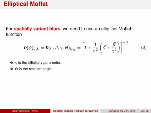
Elliptical Moffat
For spatially variant blurs, we need to use an elliptical Moffatfunction
h(φ)ix ,jy = h(α, β, γ,Θ)ix ,jy =
[1 +
1α2
(i2r +
j2rγ2
)]−β(2)
γ is the ellipticity parameter.
Θ is the rotation angle.[irjr
]=
[cos(Θ) sin(Θ)− sin(Θ) cos(Θ)
] [ixjy
].
Bob Plemmons (WFU) Spectral Imaging Through Turbulence Sanya China, Jan. 2015 28 / 52
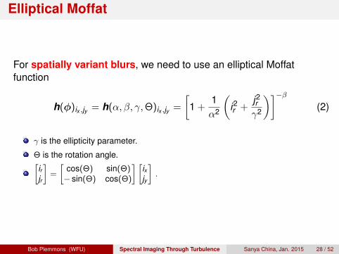
Elliptical Moffat
For spatially variant blurs, we need to use an elliptical Moffatfunction
h(φ)ix ,jy = h(α, β, γ,Θ)ix ,jy =
[1 +
1α2
(i2r +
j2rγ2
)]−β(2)
γ is the ellipticity parameter.
Θ is the rotation angle.
[irjr
]=
[cos(Θ) sin(Θ)− sin(Θ) cos(Θ)
] [ixjy
].
Bob Plemmons (WFU) Spectral Imaging Through Turbulence Sanya China, Jan. 2015 28 / 52
Elliptical Moffat
For spatially variant blurs, we need to use an elliptical Moffatfunction
h(φ)ix ,jy = h(α, β, γ,Θ)ix ,jy =
[1 +
1α2
(i2r +
j2rγ2
)]−β(2)
γ is the ellipticity parameter.
Θ is the rotation angle.[irjr
]=
[cos(Θ) sin(Θ)− sin(Θ) cos(Θ)
] [ixjy
].
Bob Plemmons (WFU) Spectral Imaging Through Turbulence Sanya China, Jan. 2015 28 / 52

Wavelength Varying Elliptical Moffat
The variation of the elliptical Moffat PSF with respect to λ and thepolar coordinates (ρ, θ) in the field of view
γ(λ, ρ) = 1 + (γ0 + γ1λ)ρ
β is kept as a constant
α(λ, ρ) = α0 + α1ρ+ α2λ+ α3λ2.
Θ = π2 − θ.
D. Serre, E. Villeneuve, H. Carfantan, L. Jolissaint, V. Mazet, S. Bourguignon, A. JarnoModeling the spatial PSF at the VLT focal plane for MUSE WFM data analysis purposeSPIE Astronomical Telescopes and Instrumentation: Observational Frontiers of Astronomyfor the New Decade (2010)
Bob Plemmons (WFU) Spectral Imaging Through Turbulence Sanya China, Jan. 2015 29 / 52

Example: Elliptical Moffat - 7 Parameters for eachλ
For λ = 465nm: α0 = 3.75, α1 = −2.99 · 10−3, α2 = −4.31 · 10−3, α3 = 1.98 · 10−6
β = 1.74, γ0 = 6.86 · 10−4, γ1 = 2.17 · 10−6
1
2
3
4
5
6
7
8
9
10
Bob Plemmons (WFU) Spectral Imaging Through Turbulence Sanya China, Jan. 2015 30 / 52

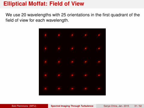
Elliptical Moffat: Field of View
We use 20 wavelengths with 25 orientations in the first quadrant of thefield of view for each wavelength.
Bob Plemmons (WFU) Spectral Imaging Through Turbulence Sanya China, Jan. 2015 31 / 52
Elliptical Moffat: Field of View
We use 20 wavelengths with 25 orientations in the first quadrant of thefield of view for each wavelength.
Bob Plemmons (WFU) Spectral Imaging Through Turbulence Sanya China, Jan. 2015 31 / 52
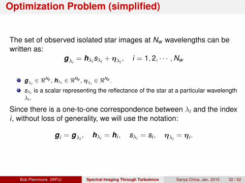
Optimization Problem (simplified)
The set of observed isolated star images at Nw wavelengths can bewritten as:
gλi= hλi sλi + ηλi
, i = 1,2, · · · ,Nw
gλi∈ <Np , hλi ∈ <
Np , ηλi∈ <Np .
sλi is a scalar representing the reflectance of the star at a particular wavelengthλi .
Since there is a one-to-one correspondence between λi and the indexi , without loss of generality, we will use the notation:
g i = gλi, hλi = hi , sλi = si , ηλi
= ηi .
Bob Plemmons (WFU) Spectral Imaging Through Turbulence Sanya China, Jan. 2015 32 / 52

Optimization Problem
By stacking all observations, we obtain the overall image formationmodel as:
g = H(φ)s + η
where
s =
s1s2...
sNw
and in the simpler case of a circular Moffat PSF,
g =
g1g2...
gNw
, H(φ) =
h1 0 · · · 0
0 h2...
.... . .
0 · · · hNw
, φ =
α0α1β
.
Bob Plemmons (WFU) Spectral Imaging Through Turbulence Sanya China, Jan. 2015 33 / 52

Optimization Problem
In the case of elliptical Moffat PSF, with Nw wavelengths and Noorientations (i.e., No polar coordinates (ρ`, θ`), ` = 1,2, . . . ,No) in thefield of view, we have
g =
g(1)1...
g(No)1
g(1)2...
g(No)2...
g(1)Nw...
g(No)Nw
, H(φ) =
h(1)1 0 · · · 0...
... · · ·...
h(No)1 0 · · · 00 h(1)
2 · · · 0...
... · · ·...
0 h(No)2 · · · 0
0 0 · · · 0...
. . ....
0 · · · h(1)Nw
.... . .
...0 · · · h(No)
Nw
, φ =
α0
α1
α2
α3
βγ0
γ1
.
Bob Plemmons (WFU) Spectral Imaging Through Turbulence Sanya China, Jan. 2015 34 / 52

Optimization Problem
We formulate the PSF parameter estimation and star spectrumreconstruction problem in a nonlinear least squares framework
minφ,s
(f (φ,s) = ‖g − H(φ)s‖22
)
Note thatf (φ, s) is linear in s and nonlinear in φ
φ ∈ <p, s ∈ <Nw and p < Nw
Variable projection method:Implicitly eliminate linear term s.
Optimize over nonlinear term φ using Gauss-Newton.
φ used to specify the spatially varying elliptical PSF parameters at eachwavelength.
Bob Plemmons (WFU) Spectral Imaging Through Turbulence Sanya China, Jan. 2015 35 / 52

Optimization Problem
We formulate the PSF parameter estimation and star spectrumreconstruction problem in a nonlinear least squares framework
minφ,s
(f (φ,s) = ‖g − H(φ)s‖22
)Note that
f (φ, s) is linear in s and nonlinear in φ
φ ∈ <p, s ∈ <Nw and p < Nw
Variable projection method:Implicitly eliminate linear term s.
Optimize over nonlinear term φ using Gauss-Newton.
φ used to specify the spatially varying elliptical PSF parameters at eachwavelength.
Bob Plemmons (WFU) Spectral Imaging Through Turbulence Sanya China, Jan. 2015 35 / 52
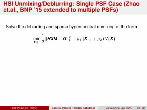
HSI Unmixing/Deblurring: Single PSF Case (Zhaoet.al., BNP ’15 extended to multiple PSFs)
Solve the deblurring and sparse hyperspectral unmixing of the form
minX≥0
12||HXM −G||2F + µ1||X ||1 + µ2TV (X )
H ∈ <Np×Np is a block diagonal blurring matrix constructed using elliptical Moffatfunction parameters from our estimate φ.
ADMM applied to compute X .
X-L. Zhao, F. Wang, T-Z. Huang, M. K. Ng, and R. J. PlemmonsDeblurring and Sparse Unmixing for Hyperspectral ImagesIEEE Transactions on Geoscience and Remote Sensing (2013).
Berisha, Nagy and Ple. “Deblurring and Sparse Unmixing of Hyperspectral Images usingMultiple PSFs,” in revision, SIAM J. Sci. Comp. 2015.
Bob Plemmons (WFU) Spectral Imaging Through Turbulence Sanya China, Jan. 2015 36 / 52
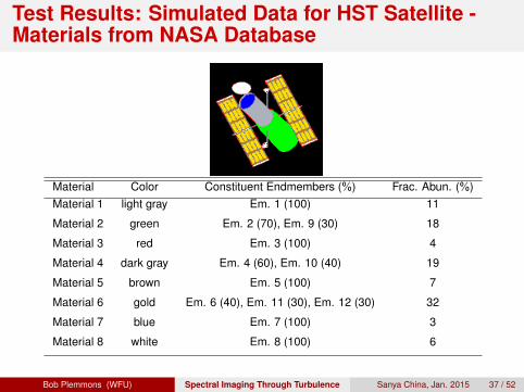
Test Results: Simulated Data for HST Satellite -Materials from NASA Database
Material Color Constituent Endmembers (%) Frac. Abun. (%)Material 1 light gray Em. 1 (100) 11
Material 2 green Em. 2 (70), Em. 9 (30) 18
Material 3 red Em. 3 (100) 4
Material 4 dark gray Em. 4 (60), Em. 10 (40) 19
Material 5 brown Em. 5 (100) 7
Material 6 gold Em. 6 (40), Em. 11 (30), Em. 12 (30) 32
Material 7 blue Em. 7 (100) 3
Material 8 white Em. 8 (100) 6
Bob Plemmons (WFU) Spectral Imaging Through Turbulence Sanya China, Jan. 2015 37 / 52

Spectral signatures of eight materials, such asaluminum, solar cell, copper tubing, etc.
500 1000 1500 2000 25000
0.2
0.4
0.6
0.8
1
500 1000 1500 2000 25000
0.2
0.4
0.6
0.8
1
500 1000 1500 2000 25000
0.2
0.4
0.6
0.8
1
500 1000 1500 2000 25000
0.2
0.4
0.6
0.8
1
500 1000 1500 2000 25000
0.2
0.4
0.6
0.8
1
500 1000 1500 2000 25000
0.2
0.4
0.6
0.8
1
500 1000 1500 2000 25000
0.2
0.4
0.6
0.8
1
500 1000 1500 2000 25000
0.2
0.4
0.6
0.8
1
Bob Plemmons (WFU) Spectral Imaging Through Turbulence Sanya China, Jan. 2015 38 / 52

Simulated data at different wavelengths
λ = 400nm λ = 1107.1nm λ = 1814.3nm
Bob Plemmons (WFU) Spectral Imaging Through Turbulence Sanya China, Jan. 2015 39 / 52

Simulated data at different wavelengths
λ = 400nm λ = 1107.1nm λ = 1814.3nm
Bob Plemmons (WFU) Spectral Imaging Through Turbulence Sanya China, Jan. 2015 39 / 52

Simulated data at different wavelengths
λ = 400nm λ = 1107.1nm λ = 1814.3nm
Bob Plemmons (WFU) Spectral Imaging Through Turbulence Sanya China, Jan. 2015 39 / 52

Relative Errors, Relative Residual Norms
0 50 100 150 2000.2
0.3
0.4
0.5
0.6
0.7
0.8
0.9
1
Iterations
Re
lative
Err
ors
Multiple PSFs
One PSF
0 20 40 60 80 10010
−7
10−6
10−5
10−4
10−3
10−2
10−1
100
Iterations
Re
lative
re
sid
ua
l n
orm
s
PCG
CG
Relative errors
Relative residual norms
Outer ADMM iterations: 200 CG iterations: 1000 PCG iterations: 20
µ1 = 0.01, µ2 = 5× 10⁻⁴, β = 0.01, Noise = 30dB
Bob Plemmons (WFU) Spectral Imaging Through Turbulence Sanya China, Jan. 2015 40 / 52

Relative Errors, Relative Residual Norms
0 50 100 150 2000.2
0.3
0.4
0.5
0.6
0.7
0.8
0.9
1
Iterations
Re
lative
Err
ors
Multiple PSFs
One PSF
0 20 40 60 80 10010
−7
10−6
10−5
10−4
10−3
10−2
10−1
100
Iterations
Re
lative
re
sid
ua
l n
orm
s
PCG
CG
Relative errors Relative residual norms
Outer ADMM iterations: 200 CG iterations: 1000 PCG iterations: 20
µ1 = 0.01, µ2 = 5× 10⁻⁴, β = 0.01, Noise = 30dB
Bob Plemmons (WFU) Spectral Imaging Through Turbulence Sanya China, Jan. 2015 40 / 52

Reconstructed Fractional Abundances
True Single PSF Multiple PSF
Bob Plemmons (WFU) Spectral Imaging Through Turbulence Sanya China, Jan. 2015 41 / 52

Reconstructed Fractional Abundances
True Single PSF Multiple PSF
Bob Plemmons (WFU) Spectral Imaging Through Turbulence Sanya China, Jan. 2015 41 / 52

Reconstructed Fractional Abundances
True Single PSF Multiple PSF
Bob Plemmons (WFU) Spectral Imaging Through Turbulence Sanya China, Jan. 2015 41 / 52

Reconstructed Fractional Abundances
True Single PSF Multiple PSF
Bob Plemmons (WFU) Spectral Imaging Through Turbulence Sanya China, Jan. 2015 42 / 52

Reconstructed Fractional Abundances
True Single PSF Multiple PSF
Bob Plemmons (WFU) Spectral Imaging Through Turbulence Sanya China, Jan. 2015 42 / 52

Reconstructed Fractional Abundances
True Single PSF Multiple PSF
Bob Plemmons (WFU) Spectral Imaging Through Turbulence Sanya China, Jan. 2015 42 / 52

Reconstructed Fractional Abundances
True Single PSF Multiple PSF
Bob Plemmons (WFU) Spectral Imaging Through Turbulence Sanya China, Jan. 2015 43 / 52

Reconstructed Fractional Abundances
True Single PSF Multiple PSF
Bob Plemmons (WFU) Spectral Imaging Through Turbulence Sanya China, Jan. 2015 43 / 52

Reconstructed Material Spectral SignaturesThe true material spectral signatures: − The computed spectral signatures: −.
500 1000 1500 2000 25000
0.2
0.4
0.6
0.8
1
500 1000 1500 2000 25000
0.2
0.4
0.6
0.8
1
500 1000 1500 2000 25000
0.2
0.4
0.6
0.8
1
500 1000 1500 2000 25000
0.2
0.4
0.6
0.8
1
500 1000 1500 2000 25000
0.2
0.4
0.6
0.8
1
500 1000 1500 2000 25000
0.2
0.4
0.6
0.8
1
500 1000 1500 2000 25000
0.2
0.4
0.6
0.8
1
500 1000 1500 2000 25000
0.2
0.4
0.6
0.8
1
Bob Plemmons (WFU) Spectral Imaging Through Turbulence Sanya China, Jan. 2015 44 / 52

In Progress – Deblurring & Feature Extraction
• Spectro-Polarimetric Compressive Sensing from SnapshotHSI-Polarization Imaging through Turbulence
• Using data from a polarimetric coded aperture snapshot spectralimager (CASSPI) camera (a 4D tensor problem) in AFOSR projectjoint with: D. Brady (ECE, Duke), S. Prasad (Physics, UNM), andSebastian Berisha (Radiology, UPenn).
• Data reconstruction and joint deblurring and feature extraction usingADMM.
Preprint later: http://users.wfu.edu/plemmons/
Bob Plemmons (WFU) Spectral Imaging Through Turbulence Sanya China, Jan. 2015 45 / 52

Snapshot Spectral & Spectro-PolarimetricCompressive Sensing - Enables HSI Video Imaging
Coded-Aperture Snapshot Spectral Imagers: DD-CASSI, SD-CASSI,CASSPI. Dave Brady et al., 2007 - present.
g(x , y) =
∫λ
Cλ(x , y)f (x , y , λ)dλ+ ελ(x , y).
Cλ(x , y) is wavelength dependent system function.
• Spatial Light Modulator (SLM)-based CASSPI - snapshotspectro-polarimetric imager forward model.
g(x , y) =∑µ
∫λ
Cµ(x , y , λ)[h(x , y , λ) ∗ fµ(x , y , λ)]dλ+ ελ,µ(x , y).
µ = polarimetric variable.
Bob Plemmons (WFU) Spectral Imaging Through Turbulence Sanya China, Jan. 2015 46 / 52

Segmentation Model
Segmentation model:
f (x , y , λ) =m∑
i=1
si(λ)ui(x , y).
Resulting system model:
g =
∫λ
Cλ(x , y)[hφλ(x , y) ∗m∑
i=1
si(λ)ui(x , y)]dλ+ ε(x , y).
Knowns: coded, blurred image g, and CASSI system operator C.Unknowns: phase function φ ( in terms of the OPD), spectralsignatures si , and support functions, ui .Approach: we take a two-step approach, that is, we estimate theoptical path difference function (OPD) first using a HSI of a guide star,and then classify features of object.
Bob Plemmons (WFU) Spectral Imaging Through Turbulence Sanya China, Jan. 2015 47 / 52

Feature Classification of Hyperspectral Objects
• Assume the OPD is known as the estimated φ̂ from Berisha, Nagy,Ple. 2014 so each PSF hλ is available. We estimate support functionsui and spectral signatures si .
J(u, s) =12
∥∥∥∥∥∫λ
Cλ(x , y)
[hλ(x , y) ∗
m∑i=1
si(λ)ui(x , y)
]− g(x , y)
∥∥∥∥∥2
2
+ α
m∑i=1
∫R2
√∇2
xxi +∇2yyi +
β
2
m∑i=1
∫λ‖si(λ)‖2,
where we use total variation regularization for ui and Tikhonov forspectral signatures si .
•Will solve inverse problem using ADMM.
Bob Plemmons (WFU) Spectral Imaging Through Turbulence Sanya China, Jan. 2015 48 / 52

Spectro-Polarimetric Camera - Duke, UNM, WFU AF Project
System modulates a 4D tensor array image onto a 2D detector(matrix). Project in progress. To reconstruct, and jointly deblur &extract features.
Bob Plemmons (WFU) Spectral Imaging Through Turbulence Sanya China, Jan. 2015 49 / 52

Epilogue
In retrospect: Did van Gogh envision atmospheric turbulence in hismost widely acclaimed painting – Starry Night?
Vincent van Gogh
Bob Plemmons (WFU) Spectral Imaging Through Turbulence Sanya China, Jan. 2015 50 / 52

Comments
Optical Imaging in Remote Sensing – 2015 is UNESCO “Year ofLight”Overview of Our Projects - NGA & AFOSR(Imaging Through) Turbulence - Galileo, Von Karman,Komolgorov, ...Hyperspectral Imaging (HSI) through Atmospheric TurbulenceEstimating HSI PSFs for Atmospheric Turbulence - HSI image ofguide star, Moffat fct. modelingJoint Deblurring and Feature Extraction - ADMM optimizationapproachOverview of Compressive Snapshot HSI - Enables HSI videoSpectro-Polarimetric Imaging - Adds polarization channels forStokes images used in identifying object shape and surfaceproperties
Bob Plemmons (WFU) Spectral Imaging Through Turbulence Sanya China, Jan. 2015 51 / 52

Thank You!
Bob Plemmons (WFU) Spectral Imaging Through Turbulence Sanya China, Jan. 2015 52 / 52