Image Vectorization using Optimized Gradient … containing both smoothly shaded and rapid changes. Also, as shown in Figure 1, optimized gradient meshes have a much simpler structure

ACM Reference FormatSun, J., Liang, L., Wen, F., Shum, H. 2007. Image Vectorization using Optimized Gradient Meshes. ACM Trans. Graph. 26, 3, Article 11 (July 2007), 7 pages. DOI = 10.1145/1239451.1239462 http://doi.acm.org/10.1145/1239451.1239462.

Copyright NoticePermission to make digital or hard copies of part or all of this work for personal or classroom use is granted without fee provided that copies are not made or distributed for profi t or direct commercial advantage and that copies show this notice on the fi rst page or initial screen of a display along with the full citation. Copyrights for components of this work owned by others than ACM must be honored. Abstracting with credit is permitted. To copy otherwise, to republish, to post on servers, to redistribute to lists, or to use any component of this work in other works requires prior specifi c permission and/or a fee. Permissions may be requested from Publications Dept., ACM, Inc., 2 Penn Plaza, Suite 701, New York, NY 10121-0701, fax +1 (212) 869-0481, or [email protected].© 2007 ACM 0730-0301/2007/03-ART11 $5.00 DOI 10.1145/1239451.1239462 http://doi.acm.org/10.1145/1239451.1239462

Image Vectorization using Optimized Gradient Meshes

Jian Sun Lin Liang Fang Wen Heung-Yeung Shum

Microsoft Research Asia

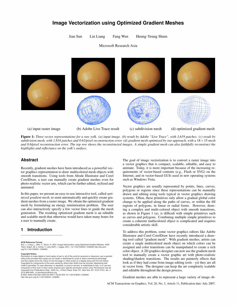
(a) input raster image (b) Adobe Live Trace result (c) subdivision mesh (d) optimized gradient mesh

Figure 1: Three vector representations for a raw yolk. (a) input image. (b) result by Adobe “Live Trace”, with 3,619 patches. (c) result bysubdivision mesh, with 1,834 patches and 0.61/pixel reconstruction error. (d) gradient mesh optimized by our approach, with a 18×15 meshand 0.6/pixel reconstruction error. The top row shows the reconstructed images. A simple gradient mesh can also faithfully reconstruct thehighlights and reflectance on the yolk’s surface.

Abstract

Recently, gradient meshes have been introduced as a powerful vec-tor graphics representation to draw multicolored mesh objects withsmooth transitions. Using tools from Abode Illustrator and CorelCorelDraw, a user can manually create gradient meshes even forphoto-realistic vector arts, which can be further edited, stylized andanimated.

In this paper, we present an easy-to-use interactive tool, called opti-mized gradient mesh, to semi-automatically and quickly create gra-dient meshes from a raster image. We obtain the optimized gradientmesh by formulating an energy minimization problem. The usercan also interactively specify a few vector lines to guide the meshgeneration. The resulting optimized gradient mesh is an editableand scalable mesh that otherwise would have taken many hours fora user to manually create.

1 Introduction

The goal of image vectorization is to convert a raster image intoa vector graphics that is compact, scalable, editable, and easy toanimate. Today, it is more important because of the increasing re-quirements of vector-based contents (e.g., Flash or SVG) on theInternet, and in vector-based GUIs used in new operating systemssuch as Windows Vista.

Vector graphics are usually represented by points, lines, curves,polygons or regions since these representations can be manuallydrawn and editing using tools typical in vector graphics drawingsystems. Often, these primitives only allow a gradual global colorchange to be applied along the paths of curves, or within the fillregions of polygons, in linear or radial forms. However, draw-ing a complex and multi-colored object with smooth transitions,as shown in Figure 1 (a), is difficult with simple primitives suchas curves and polygons. Combining multiple simple primitives tocreate a coherent multicolored object is complicated and requiresconsiderable artistic skill.

To address this problem, some vector graphics editors like AdobeIllustrator and Corel CorelDraw have recently introduced a draw-ing tool called “gradient mesh”. With gradient meshes, artists cancreate a single multicolored mesh object on which colors can beassigned and color transitions can be manipulated to create a richcolor object. A 2D graphics designer can now use the gradient meshtool to manually create a vector graphic art with photo-realisticshading/shadow transitions. The results are painterly effects thatlook as if they had come from image editing tools - yet they are allin vector form. The designer can keep the art completely scalableand editable throughout the design process.

Gradient meshes are able to represent a large variety of image ob-

ACM Transactions on Graphics, Vol. 26, No. 3, Article 11, Publication date: July 2007.

jects containing both smoothly shaded and rapid changes. Also, asshown in Figure 1, optimized gradient meshes have a much simplerstructure and thus are easier for the user to edit than those createdby other vectorization methods. However, it is often tedious andtime-consuming to delineate an object with photo-realistic gradualtransitions from a real image. It can easily take more than an hourby a professional artist using the gradient mesh tool to manuallycreate a simple mesh like Figure 1(d).

In this paper, we provide a tool, called “optimized gradient mesh”,to help a user to quickly convert an image object into gradientmeshes. It only requires a small amount of user assistance for ini-tialization. Figure 1 (d) shows an optimized gradient mesh createdby our approach in less than a minute. Our tool works well withmulticolored objects with smooth shading or shadow transitions,such as a face, a body, a toy, a piece of art, or any object with asmooth surface, in real images. The optimized gradient mesh is alsoable to handle a moderate amount of rapid color/intensity changes.For example, the highlights and complex reflectance on the yolk’ssurface are faithfully reconstructed in Figure 1 (d).

While the gradient mesh exists in commercial tools, we are the firstto introduce it for image vectorization. We also present an effectiveoptimization approach to fit gradient meshes to an image. Gradientmeshes produced by our technique have several advantages: 1) Ef-ficiency of use; the optimized gradient mesh makes it much fasterfor users to create gradient meshes from an input image. A skill-ful artist can save substantial labor and focus on re-creation, and anovice is able to create a single or a library of photo-realistic vectorart for re-use. 2) Easy to edit; compared with other vectorizationtools, the optimized gradient mesh can produce a simpler mesh thatthe user can further edit and animate. 3) Scalability; The gradientmeshes can be scaled in size with fewer artifacts, as we will explainin Section 3.1. 4) Compact representation. The gradient mesh is anefficient representation for image objects with smooth transitions.For example, Figure 1 (d) shows a 7.7KB mesh, whereas the samequality JPEG image is 37.5KB. This advantage will be increased ifthe object is scaled in size.

The above advantages arise from the powerful representation abilityof the gradient mesh, which introduces geometric and color gradi-ents on each vertex of the mesh and represents an image as a sparseset of points and gradients.

2 Previous Work

For scanned line art, black-white images, maps, and cartoon draw-ings, the main task of vectorization is to recognize and extract lines,regions, and text [Fan et al. 1995; Dori and Liu 1999; Zou andYan 2001; Hilaire and Tombre 2006]. These approaches are mainlybased on thresholding, thinning, contour tracing, and skeletoniza-tion algorithms in image processing. The extracted line, image con-tour, or region is represented by vector graphics primitives, e.g.,curves and paths.

Recent commercial vectorization software, such as Adobe “LiveTrace”, Corel CorelTrace, and AutoTrace [AutoTrace 2004], areable to process photographic images, but are limited to cartoon-likeflat shading images. For real images with smooth shading, theseapproaches typically output an over-segmented vector graphic con-sisting of a large number of irregular regions with flat colors. Thiskind of result is challenging to edit further. Figure 1 (b) shows aLive Trace result which contains thousands of small patches.

In RaveGrid [Swaminarayan and Prasad 2006], a constrained De-launay triangulation of the edge contour set is performed to yielda polygon based vectorization. Adaptive triangulations [Demaretet al. 2006] approximate the image as a linear spline over an adapted

m0 m1

m2m3

m(u,v)m0

v

m0u

−αqu mq

u

mqumq

v

−αqv mq

v

qq−1 q+1

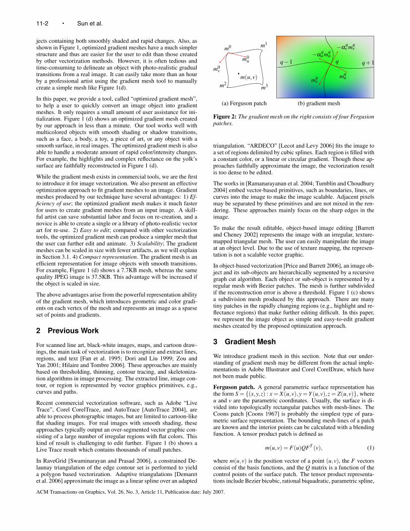
(a) Ferguson patch (b) gradient mesh

Figure 2: The gradient mesh on the right consists of four Fergusionpatches.

triangulation. “ARDECO” [Lecot and Levy 2006] fits the image toa set of regions delimited by cubic splines. Each region is filled witha constant color, or a linear or circular gradient. Though these ap-proaches faithfully approximate the image, the vectorization resultis too dense to be edited.

The works in [Ramanarayanan et al. 2004; Tumblin and Choudhury2004] embed vector-based primitives, such as boundaries, lines, orcurves into the image to make the image scalable. Adjacent pixelsmay be separated by these primitives and are not mixed in the ren-dering. These approaches mainly focus on the sharp edges in theimage.

To make the result editable, object-based image editing [Barrettand Cheney 2002] represents the image with an irregular, texture-mapped triangular mesh. The user can easily manipulate the imageat an object level. Due to the use of texture mapping, the represen-tation is not a scalable vector graphic.

In object-based vectorization [Price and Barrett 2006], an image ob-ject and its sub-objects are hierarchically segmented by a recursivegraph cut algorithm. Each object or sub-object is represented by aregular mesh with Bezier patches. The mesh is further subdividedif the reconstruction error is above a threshold. Figure 1 (c) showsa subdivision mesh produced by this approach. There are manytiny patches in the rapidly changing regions (e.g., highlight and re-flectance regions) that make further editing difficult. In this paper,we represent the image object as simple and easy-to-edit gradientmeshes created by the proposed optimization approach.

3 Gradient Mesh

We introduce gradient mesh in this section. Note that our under-standing of gradient mesh may be different from the actual imple-mentations in Adobe Illustrator and Corel CorelDraw, which havenot been made public.

Ferguson patch. A general parametric surface representation hasthe form S = {(x,y,z) : x = X(u,v),y = Y (u,v),z = Z(u,v)}, whereu and v are the parametric coordinates. Usually, the surface is di-vided into topologically rectangular patches with mesh-lines. TheCoons patch [Coons 1967] is probably the simplest type of para-metric surface representation. The bounding mesh-lines of a patchare known and the interior points can be calculated with a blendingfunction. A tensor product patch is defined as

m(u,v) = F(u)QFT (v), (1)

where m(u,v) is the position vector of a point (u,v), the F vectorsconsist of the basis functions, and the Q matrix is a function of thecontrol points of the surface patch. The tensor product representa-tions include Bezier bicubic, rational biquadratic, parametric spline,

11-2 • Sun et al.


Figure 3: Scalability. Left: a gradient mesh at original resolution(x 1). Middle: gradient mesh scaling result (x 8). Sharp edges arewell preserved. Right: bi-cubic raster scaling result (x 8). Blockyartifacts appear.

B-splines, and so on. Most of these representations are suitable forinteractive surface design, but not for describing existing surfaces,since they require control points lying outside the surface. The Fer-guson patch [Ferguson 1964; Farin 1997], however, is defined withcontrol points lying on the surface. Because of this it is suitable forimage vectorization purposes. The Ferguson patch is defined by

m(u,v) = F(u)QFT (v) = UCQCTV, (2)

where

Q =

⎡⎢⎢⎣

m0 m2 m0v m2

vm1 m3 m1

v m3v

m0u m2

u m0uv m2

uvm1

u m3u m1

uv m3uv

⎤⎥⎥⎦ , C =

⎡⎢⎣

1 0 0 00 0 1 0−3 3 −2 −1−2 2 1 1

⎤⎥⎦ ,

U =[

1 u u2 u3], and V =

[1 v v2 v3

].

The mu, mv, muv are the partial derivatives. In practice, the valuesof muv are usually set to zero. Figure 2 (a) shows a Ferguson patch.

3.1 Gradient mesh

A gradient mesh consists of topologically planar rectangular Fer-guson patches with mesh-lines. It has four boundaries and eachboundary consists of one or more cubic Bezier splines. Figure 2 (b)is a gradient mesh. For each control point q in the mesh, three typesof variables can be interactively edited: position, derivatives, andRGB color:

• the 2D position {xq,yq} of point q.

• the derivatives {mqu,m

qu,αq

u mqu,αq

u mqu} are specified by four

direction handles, as shown in Figure 2 (red lines). The direc-tion handles can be dragged as in standard path tools. In orderto achieve continuity between neighboring patches, mq

u andαq

u mqu (mq

v and αqv mq

v) have the same direction but can be dif-ferent in length, where αq

u (αqv ) is a scale variable. These four

derivatives are shared with four adjacent Ferguson patches.

• the RGB color cq = {cq(r),cq(g),cq(b)} is assigned by sam-pling a color from an input image or a color palette.

To render each colored Ferguson patch, color derivatives {cqu,c

qv}

for each channel are also necessary. In the gradient mesh tool, thesecolor derivatives are automatically estimated. Without knowing theimplementation details in Adobe Illustrator or Corel CorelDraw, wehave compared a number of methods to estimate the color deriva-tives from given colors on mesh points. We have found that a mono-tonic (1D) cubic spline interpolation [Wolberg and Alfy 1999] ofcolors along the mesh lines produces numerically similar renderingresults compared with the rendering results by Adobe Illustrator.For the example in Figure 2 (b), two cubic splines are fitted alongthe mesh line {q − 1,q,q + 1} using the monotonic cubic spline

Figure 4: Optimization. Left: a screen snapshot of a gradient meshin Adobe Illustrator. We rasterize it as our input image. Middleand Right: optimized gradient mesh. The reconstruction error is0.7/pixel.

interpolation algorithm [Wolberg and Alfy 1999]. Then the colorderivatives cq

u, cq−1u and cq+1

u are analytically calculated from thecubic splines. Each color channel is processed independently.

After getting the information (positions, geometric derivatives, col-ors, and color derivatives) of all control points, each Ferguson patchin the gradient mesh is rendered according to Equation (2):

f (u,v) = UCQ f CTV, (3)

where Q f contains color control variables. In Figure 2 (b), asmooth, multicolored image is generated by assigning the top-leftpoint as orange-red, the middle-center point as green, the bottom-center point as blue, and the other points as light gray.

By representing an image object by a sparse set of points and gra-dients, gradient meshes are compact, scalable, and editable.

Scalability. Gradient meshes can be scaled with fewer artifacts thanimages. Sharp edges whin an image object can be preserved byplacing two closely-spaced mesh lines on either side of the edge.Although a Ferguson patch is continuous in parametric coordinatespace, the derivatives of image coordinates w.r.t. parametric coor-dinates (e.g., dx/du) can change from positive to negative or vice-versa. Therefore, when we render the image by incrementally sam-pling the parametric coordinates, we may visit the same image pixeltwice and assign different colors, resulting in color discontinuities.Gradient mesh users often take advantage of this feature to draw anobject with sharp edges (as shown in Figure 3).

Gradient mesh editing. Gradient meshes are easier to manipulatethan images. The user can add, delete or edit mesh points and meshlines. For each mesh point, its derivatives are manipulated by drag-ging four direction handles. With a selected mesh point, the usercan choose a color from the color palette to define the color for thatpoint. Each mesh point’s direction handles and paths define howthis point’s color blends with other colors from other mesh points.

4 Optimized Gradient Mesh

In this section, we present our vector graphics creation tool: theoptimized gradient mesh. We denote the gradient mesh as M ={Qp,Q

fp}P

p=1, which consists of P patches. Given a smooth rasterimage object I, we expect to create or optimize a simple gradientmesh M with small reconstruction error. It is straightforward tominimize the following energy function:

E(M) =P

∑p=1

∑u,v

||Ip(m(u,v))− fp(u,v)||2 (4)

where u,v are discrete parametric coordinates in each patch p andIp is the image region in the patch p. This energy term is the recon-struction residual between the input image and the color graphics

Image Vectorization using Optimized Gradient Meshes • 11-3


Figure 5: Smoothness constraint. Left: input image. Middleand Right: optimized results without and with the smoothness con-straint. The reconstruction errors are 1.8/pixel and 0.9/pixel.

rendered by the gradient mesh using Equation (3). This fitting prob-lem is similar to geometric modeling work such as [Schmitt et al.1986; Krishnamurthy and Levoy 1996]. In this work, we fit a set ofconnected Ferguson patches to an image.

4.1 Optimization

Notice that minimizing E(M) is a non-linear least squares(NLLS) problem, i.e., the energy can be written in the formE = ∑ak||fk(z)||2, where z is the vector form of unknownsin M. For each control point, the associated unknowns are{x,y,mu,mv,αu,αv,cu,cv}. To enforce the differentiability of therendered image, the scale variables αu,αv are shared with the colorderivatives in all color channels. The color value c is a functionof (x,y) and is sampled from the underlying image, i.e., c = I(x,y).For object boundaries, the color is sampled from the estimated fore-ground colors by the coherent matting method [Shum et al. 2004]in a narrow band along the boundaries.

The Levenberg-Marquardt (LM) algorithm [Levenberg 1944] hasproven to be the most successful solver for NLLS due to its use ofan effective damping strategy that lends it the ability to convergepromptly from a wide range of initial guesses. For more detailsof the LM algorithm, please refer to [Nocedal and Wright 1999].LM requires the computation of a Jacobian (Jk)i = ∂ fk(z)

∂ zi. Since

fk(z) contains an image observation, the derivative of the image isrequired and computed by convolution with a derivative of Gaus-sian filter. Notice that the Jacobian matrix is block-sparse becauseeach Jk is only dependent on its neighboring control points. Weuse a standard LM implementation with sparse matrix support. Inorder to avoid local minima and make the solver robust, we build aGaussian pyramid from the input image and apply a coarse-to-fineoptimization for LM. The optimization time is about 10-30 secondsfor a 10× 10 mesh with our current unoptimized implementation.More sophisticated LM variants or GPU acceleration could be usedfor further speedup.

Figure 4 shows an example of an optimized gradient mesh. Wefirst manually create a gradient mesh in Adobe Illustrator. It is thenrasterized to an image as our input. The mesh is initialized by a4× 4 evenly divided mesh. Figure 4 (b) is the optimized gradientmesh after 40 LM iterations. The optimized mesh-lines are similarto the manually created mesh-lines, and the rendering results arevirtually identical. Notice that both smooth regions and sharp edgesare faithfully reconstructed.

Smoothness constraint. However, for complex examples or realimages with noise, the optimization of energy function (4) oftenbecomes stuck in a local minimum. The middle column of Figure5 shows such an example. The user also expects a smooth opti-mized mesh since the manually created gradient meshes are usually

Figure 6: From left to right: input image and initial mesh, directlyoptimized gradient mesh with reconstruction error of 2.5/pixel, twovector lines on u direction are specified by the user, optimized gra-dient mesh with vector lines as soft constraints with reconstructionerror of 0.5/pixel.

smooth. Hence, we add a smoothness term into the energy:

E ′(M) = E(M)+λP

∑p=1

∑s,t

[||m(s−Δs, t)−2m(s, t)+m(s+Δs, t)||2

+||m(s, t −Δt)−2m(s, t)+m(s, t −Δt)||2], (5)

where s and t are discrete parametric coordinates. And Δs and Δt aresampling intervals which are set as 5 times the sampling intervals ofu and v, respectively. The parameter λ balances the influence of thetwo terms, and the default value of λ is 50. Note that smoothnessis also enforced between neighboring patches, i.e., mp(−Δs, t) =mp−1(1−Δs, t), where p and p−1 are two adjacent patches in theu direction. The new energy term is the smoothness of the gradientmesh which minimizes the second-order finite difference. The lastcolumn of Figure 5 shows the optimized gradient mesh with thesmoothness constraint. Smaller reconstruction errors are obtainedby arriving at a better local minimum.

Boundary constraint. The boundary of a gradient mesh consists offour segments. Each segment is one or more cubic Bezier splines.We will describe the boundary initialization in section 4.3. In theoptimization, we want to enforce a boundary constraint in whichthe control points on the boundary only move along the splines. Forexample, for the control point q on the spline S in the u direction,the associated unknowns are reduced to {t,mv,cu,cv}, where t isthe parametric coordinate of the control point on the spline. Thescale αv should be one, and variables mu and αu are a function oft. Supposing that the two adjacent control points of q are q−1 andq+1, we have mu = ∂S

∂ t (tq+1− tq) and αu = (tq− tq−1)/(tq+1− tq),where ∂S

∂ t is the derivative of the spline S. The boundary constraintin the v direction is similarly enforced.

4.2 Vector line guided optimized gradient mesh

In most cases (all examples shown in the paper), our optimizationcan generate satisfactory results automatically. We also allow theuser to draw a few vector lines in the image to control the meshgeneration, e.g., the dominant directions of mesh-lines. Formally,if vector fields Vu and Vv along the u and v directions are specified,we optimize an energy E ′′(M) by adding a new term:

E ′′(M) = E ′(M)+βP

∑p=1

∑u,v

[wu(m(u,v))〈∂m(u,v)

∂u,⊥Vu(m(u,v))〉2

+wv(m(u,v))〈∂m(u,v)∂v

,⊥Vv(m(u,v))〉2], (6)

where 〈·〉 is the dot-product operator, ∂m(u,v)∂u is the derivative in the

u direction, and ⊥Vu(m(u,v)) is the unit normal vector of the Vu

at location m(u,v). ∂m(u,v)∂v and ⊥Vv(m(u,v)) are similarly defined.

11-4 • Sun et al.


Figure 7: Red pepper. Left: gradient meshes by an artist. Middle:initial gradient meshes. Right: optimized gradient meshes. Afterthe optimization, the highlight and shadow regions are faithfullyreconstructed.

The default value of β is 20. The new energy term encourages con-sistency between optimized mesh-lines and specified vector fields.

The vector field is only computed in a narrow band along the vectorline. The width of the narrow band is set as one fifth of the lengthof the vector line. The weight wu(m(u,v)) in Equation (6) is theGaussian falloff factor: wu(m(u,v)) = G(d|0,σ2

v ) where d is thedistance from the location m(u,v) to the nearest vector line. We setthe standard deviation σv to one third of the width of the narrowband. Figure 6 compares the optimized gradient meshes with andwithout the vector lines as soft constraints.

4.3 Mesh initialization

As drawn by artists, a complex object usually consists of severalsemantic parts. We first decompose the input image object intoseveral sub-objects using an interactive image cutout tool [Li et al.2004] or a free lasso tool. Then, the boundary of each sub-objectis manually divided into four segments. To obtain a good result, itis better to have a division so that the segments follow the majorand minor axes of the object. Each segment is fitted by one or morecubic Bezier splines. Finally, the mesh-lines are initialized in twoways: evenly distributed or interactive placement.

Each sub-object with four segments is treated as a Coons patch,which supports multiple splines on one segment. To create anevenly distributed mesh, we simply divide the Coons patch evenlyin parametric u and v coordinates. To interactively initialize a mesh,the user clicks a point p in the Coons patch, then we compute theparametric coordinates of p - (up, vp) using subdivision. A mesh-line in the u direction can be added by fixing the v coordinate tovp. Adding a mesh-line in the v direction or two mesh-lines in bothdirections can be done in a similar way.

The user can quickly create an initial mesh by simple mouse clicks.Placing more mesh-lines in rapidly changing regions and fewermesh-lines in smooth regions usually produces a better result. Butaccurate mesh-line placement and editing are not required. Themesh initialization is very quick — 1-2 minutes on average. Theinitial mesh rendering result without optimization is also shown onthe screen for instant feedback. The initial meshes of grapes (thethird row) and face (the fourth row) are shown in Figure 8.

5 Experimental Results

We first show an optimized result from a vector object created bythe gradient mesh tool in Adobe Illustrator, as shown in Figure 7.An artist drew this object using six meshes with 354 patches, andour optimized meshes consist of three meshes with 276 patches.

Boundary Init. Mesh Init. Optimization(mins) (mins) (mins)

Fig.1 - egg 1 0.2 2.2Fig.7 - pepper 3 1.5 2.8Fig.8 - cup 2 0.5 1.9Fig.8 - flower 3 1.5 2.4Fig.8 - grapes 4 2.0 11.3Fig.8 - sculpture 3 1.5 9.3Fig.8 - face 4 2.5 10.3

Table 1: Timings of examples in Figure 1, 7, and 8.

To fit the shadow region on the ground, the occluded region is in-painted. In the rendering, supersampling is applied along the ob-ject boundaries to reduce alisasing artifacts. Then, we compare ourapproach with subdivision meshes [Price and Barrett 2006] in thetop row of Figure 8. The subdivision meshes contain 1,973 smallpatches while our optimized gradient meshes consist of only 177patches without sacrificing visual quality.

Figure 8 also shows the vectorization results for a flower, grapes, asculpture, and a human face. In the flower example, five gradientmeshes are individually optimized for the five petals which are seg-mented with overlap. The user spent 3 mins to specify boundariesand 1.5 min to initialize the meshes. The optimization takes 2.5mins in total. The last two columns show editing results. We locallychange the colors of a number of mesh points and deform a fewmesh-lines to obtain naturally smooth transitions. In the next exam-ple, we separated the grapes into eight pieces. In the face example,the result consists of seven meshes - face(1), eyes(2), neck(1), rightear(1), and others(2). Note that the rendering results of the eye-brows, eyelashes, and hairs are smooth because these highly tex-tured regions are beyond the capability of the gradient mesh. In thelast example, the body of a sculpture is fitted with three overlappedgradient meshes. Table 1 shows the timings of boundary initializa-tion, mesh initialization, and mesh optimization for seven examplesin the paper.

With gradient meshes, the user can manipulate or control thesmooth transitions of colors. Moreover, animation effects can beachieved by linear interpolation of meshes. Figure 9 shows threeedited keyframes for an animation effect.

6 Conclusions

In this paper, we have introduced gradient mesh as an image rep-resentation and present an optimized gradient mesh tool for imagevectorization. The output gradient meshes are simple, quick to cre-ate, and easy for editing and animation. It is a new application ofgeometric modeling tools in the image domain.

Limitations remains in our approach. A simple gradient mesh isinsufficient to capture the fine image details and highly texturedregions, as shown in Figure 10. Another difficult case is whenthe boundaries of the object are too complicated, or the object hascomplicated topologies, very thin structures, or many small holes.Despite these limitations, our optimized gradient mesh extends therange of “editable” vectorization to a variety of images.

AcknowledgementsWe thank the anonymous reviewers for helping us to improve thispaper, and Stephen Lin for his help in video production and proof-reading. This work is inspired by Alex Hsu’s talk at Microsoft Re-search Asia.



Figure 8: More examples on real images. From left to right: input image, reconstruction result, and optimized gradient meshes. In the toprow, the third column shows the subdivision mesh result. In the second row, the last two columns are the edited rendering result and mesh. Inthe third row, the third column is the initial mesh that is evenly distributed. In the fourth row, the third column is the interactively initializedmesh. From top to bottom: teacup (2 meshes, 177 patches), flower (5 meshes), grapes (8 meshes), face (7 meshes), and sculpture (4 meshes).The reconstruction errors of all examples are below 1.0/pixel.

11-6 • Sun et al.


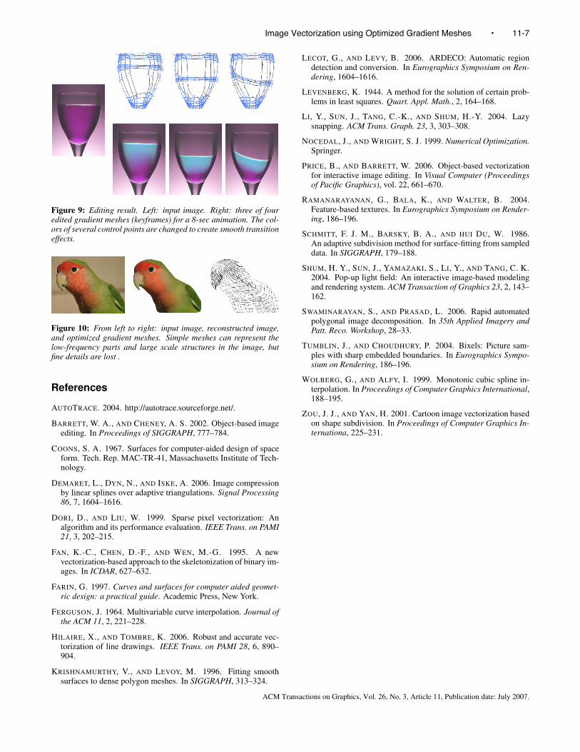
Figure 9: Editing result. Left: input image. Right: three of fouredited gradient meshes (keyframes) for a 8-sec animation. The col-ors of several control points are changed to create smooth transitioneffects.

Figure 10: From left to right: input image, reconstructed image,and optimized gradient meshes. Simple meshes can represent thelow-frequency parts and large scale structures in the image, butfine details are lost .

References

AUTOTRACE. 2004. http://autotrace.sourceforge.net/.

BARRETT, W. A., AND CHENEY, A. S. 2002. Object-based imageediting. In Proceedings of SIGGRAPH, 777–784.

COONS, S. A. 1967. Surfaces for computer-aided design of spaceform. Tech. Rep. MAC-TR-41, Massachusetts Institute of Tech-nology.

DEMARET, L., DYN, N., AND ISKE, A. 2006. Image compressionby linear splines over adaptive triangulations. Signal Processing86, 7, 1604–1616.

DORI, D., AND LIU, W. 1999. Sparse pixel vectorization: Analgorithm and its performance evaluation. IEEE Trans. on PAMI21, 3, 202–215.

FAN, K.-C., CHEN, D.-F., AND WEN, M.-G. 1995. A newvectorization-based approach to the skeletonization of binary im-ages. In ICDAR, 627–632.

FARIN, G. 1997. Curves and surfaces for computer aided geomet-ric design: a practical guide. Academic Press, New York.

FERGUSON, J. 1964. Multivariable curve interpolation. Journal ofthe ACM 11, 2, 221–228.

HILAIRE, X., AND TOMBRE, K. 2006. Robust and accurate vec-torization of line drawings. IEEE Trans. on PAMI 28, 6, 890–904.

KRISHNAMURTHY, V., AND LEVOY, M. 1996. Fitting smoothsurfaces to dense polygon meshes. In SIGGRAPH, 313–324.

LECOT, G., AND LEVY, B. 2006. ARDECO: Automatic regiondetection and conversion. In Eurographics Symposium on Ren-dering, 1604–1616.

LEVENBERG, K. 1944. A method for the solution of certain prob-lems in least squares. Quart. Appl. Math., 2, 164–168.

LI, Y., SUN, J., TANG, C.-K., AND SHUM, H.-Y. 2004. Lazysnapping. ACM Trans. Graph. 23, 3, 303–308.

NOCEDAL, J., AND WRIGHT, S. J. 1999. Numerical Optimization.Springer.

PRICE, B., AND BARRETT, W. 2006. Object-based vectorizationfor interactive image editing. In Visual Computer (Proceedingsof Pacific Graphics), vol. 22, 661–670.

RAMANARAYANAN, G., BALA, K., AND WALTER, B. 2004.Feature-based textures. In Eurographics Symposium on Render-ing, 186–196.

SCHMITT, F. J. M., BARSKY, B. A., AND HUI DU, W. 1986.An adaptive subdivision method for surface-fitting from sampleddata. In SIGGRAPH, 179–188.

SHUM, H. Y., SUN, J., YAMAZAKI, S., LI, Y., AND TANG, C. K.2004. Pop-up light field: An interactive image-based modelingand rendering system. ACM Transaction of Graphics 23, 2, 143–162.

SWAMINARAYAN, S., AND PRASAD, L. 2006. Rapid automatedpolygonal image decomposition. In 35th Applied Imagery andPatt. Reco. Workshop, 28–33.

TUMBLIN, J., AND CHOUDHURY, P. 2004. Bixels: Picture sam-ples with sharp embedded boundaries. In Eurographics Sympo-sium on Rendering, 186–196.

WOLBERG, G., AND ALFY, I. 1999. Monotonic cubic spline in-terpolation. In Proceedings of Computer Graphics International,188–195.

ZOU, J. J., AND YAN, H. 2001. Cartoon image vectorization basedon shape subdivision. In Proceedings of Computer Graphics In-ternationa, 225–231.



Documents

Image Vectorization using Optimized Gradient … containing both smoothly shaded and rapid changes. Also, as shown in Figure 1, optimized gradient meshes have a much simpler structure