Image Synthesis using Adjoint Photons

R. Keith Morley

Princeton University

Solomon Boulos

University of Utah

Jared Johnson

University of Central Florida

David Edwards

University of Utah

Peter Shirley

University of Utah

Michael Ashikhmin

SUNY Stony Brook

Simon Premoze

ILM

Figure 1: An image generated using adjoint photon tracing in a scene with millions of instanced polygons, a heterogeneous medium fromsimulation data, and Rayleigh scattering for the sky. The Sun is the only source of light in the scene (i.e. there is no background radiance orsky map) and uses a spectral radiance emission function.

ABSTRACT

The most straightforward image synthesis algorithm is to followphoton-like particles from luminaires through the environment.These particles scatter or are absorbed when they interact with asurface or a volume. They contribute to the image if and when theystrike a sensor. Such an algorithm implicitly solves the light trans-port equation. Alternatively, adjoint photons can be traced fromthe sensor to the luminaires to produce the same image. This “ad-joint photon” tracing algorithm is described, and its strengths andweaknesses are discussed, as well as details needed to make adjointphoton tracing practical.

Keywords: global illumination, adjoint Monte Carlo methods

1 INTRODUCTION

In this paper we discuss tracing adjoint photons to create images.This method of image synthesis has some theoretical and practicaladvantages over path tracing [9]; it is simpler to motivate becauseless of the machinery of radiometry and Monte Carlo integrationare needed, and lacking ray integration and explicit direct lightingit deals better with some “difficult” scenes. Our paper developssome of the details of adjoint photon tracing, and discusses whereit needs improvement.

Our motivation for this work is three-fold. First, we have foundthat for predictive engineering applications (e.g. accurately simulat-ing a car headlight modeled as a glass case over a curved, specular

reflector in a fog bank), both the geometric and optical complex-ity can overwhelm most renderers. Second, as complex renderersadopt layers of tricks, approximations, and hacks, both their designelegance and robustness suffer. Finally, we note that in a world ofinteractive ray tracing, a batch renderer can send trillions of raysin an overnight run. Such a budget obviates the need for many ap-proximations in applications that benefit from higher accuracy. Allthree of these motivations imply that we should explore simple al-gorithms with high generality and straightforward implementation.

The particular algorithm we have choosen is to send photonsfrom the sensor (pixel) into the environment and note how likelythis is to hit the light source. This is like path tracing in that it sendsrays from the sensor into the environment and lets them chooserandom directions, but it has three important differences from pathtracing all of which are advantages in complex scenes where pre-dictive results are desired:

• indirect and direct lighting are not separated so there are noexplicit shadow rays making luminaires with reflectors notany more difficult than diffusely emitting surfaces;

• all adjoint photons have exactly one wavelength rather thancarrying a spectrum, so bidirectional reflection distributionfunctions (BRDFs) and phase functions that vary in shapewith wavelength present no particular difficulties;

• volumes are probabilistically either hit or not hit by adjointphotons so their transparency is accounted for by the percent-age of adjoint photons that hit rather than by accumulationof opacity for each adjoint photon, resulting in a straightfor-ward implementation well-suited to problems requiring manysamples per pixel.

sensorplane

752nm

540nm

585nm

Photons

lens

light

420nm

Adjoint Photons

lens

sensor(weighting function w)

light(density e)

Figure 2: The light emits spectral radiance e and the sensor weightsincident light with function w. Left: Photons are traced from the lightwith cosine-weighted e(~x,ω,λ , t) as the emitted radiance and onlyrecorded with w(~x,ω,λ , t) when they hit the sensor. Right: Adjointphotons are traced from the sensor with cosine-weighted w(~x,ω,λ , t)as the emitted radiance and only recorded with e(~x,ω,λ , t) when theyhit the light. These processes both result in the same accumulatedresponse with no need for conversion factors between units. In thisexample, the adjoint photon case is equivalent to using a planar lightsource behind the lens and a spherical camera.

2 ADJOINT LIGHT TRANSPORT

While the self-adjoint nature of light transport has been exploited ingraphics for over a decade [5, 13, 18], it has a longer history in othertransport problems as surveyed in the excellent articles by Arvo [1]and Christensen [4]. However, a physical implication of this self-adjoint property is not as well known: the emission of a light sourceand the response of a sensor can be exchanged without changingthe throughput along a path. This property has been exploited ingraphics for the first time indual photography [16] but also makesthe design of a rendering algorithm straightforward.

This exchange of source emission and sensor response does notjust mean that some kind of “importance” can be emitted from thelight, but that a complete exchange can take place without any nor-malization. That is, suppose we have a luminaire whose emittedspectral radiance is given by a functione(~x,ω,λ , t), where~x is a3D location,ω is the emitted direction of light,λ is wavelengthandt is time. Further suppose we have a sensor which responds toincident spectral radianceL with the integral:

R =∫

w(~x,ω,λ , t)L(~x,ω,λ , t)cosθdAdΩdλ dt

whereR is the response of the sensor andw is the weighting func-tion for the sensor. Note thatR depends on bothe and the propertiesof the environment. In a typical environment,e is non-zero on anyluminaire surface during whatever time period it is “on”. The sen-sor weightw is non-zero on the sensor element (e.g. a CCD pixel)during the time the sensor is active.

If we were to make the sensor emit light with spectral radiancew(~x,ω,λ , t) and make the luminaire a sensor with weighting func-tion e(~x,ω,λ , t) the resulting response is:

RA =∫

e(~x,ω,λ , t)L(~x,ω,λ , t)cosθdAdΩdλ dt.

The key property that reversibility implies is that this response isexactly the same as the original case:

RA = R.

An immediate implication of this is that any rendering program canbe “run in reverse” by emitting light from sensors using the sensorresponse as an emitted radiance distribution, and sensing that lightat luminaires using their radiance distribution as sensitivity. Thisrequires no additional normalization or complicated equations. Weexploit this in the next section using photon tracing.

3 ADJOINT PHOTON TRACING

The simplest algorithm is a brute-force simulation of photon-likeparticles as illustrated in the left of Figure 2. This differs fromthe family of photon-tracing algorithms that store photon-surfaceand photon-volume intersections [7] in that nothing is logged butinteractions with the sensor array. The tracing of photons (as op-posed to how they are logged) is the same as that of Walter etal. [23] where photons have individual wavelengths so wavelength-dependent scattering is straightforward. The algorithm to computethe sensor responseR is:

R = 0Q =

∫e(~x,ω,λ , t)cosθ dAdΩdλ dt

for each of N photons dochoose a random (~x,ω,λ , t) ∼ e(~x,ω,λ , t)cosθ/Qwhile photon is not absorbed do

find point ~x′ hit by rayR = R+(Q/N)w(~x′,ω,λ , t)H =

∫ρ(~x′,ω ′,ω,λ , t)cosθ ′ dA′ dΩ′ dλ dt

if random < H thenchoose random ω ′

∼ ρ(~x′,ω ′,ω,λ , t)cosθ ′/Helse

absorb photon

Hereρ is the BRDF,e is the emitted spectral radiance as defined inthe last section, andw is the sensor response function as defined inthe last section. The lineR = R+Qw(~x,ω,λ , t) has no cosine termbecause it is included implicitly by the change in projected area ofthe sensor which varies linearly with cosine. Note that bothe andw are defined over all surfaces, butw is non-zero only on the sensorande is non-zero only on the luminaires. Thus no photons are gen-erated except at luminaires, and only photons hitting a sensor affectthe value of the sensor valueR. The constantsH andQ simply serveas normalization factors to ensure thate andρ are valid probabilitydensity functions (pdfs). Note that the valueR is a scalar, just as forone element in a typical CCD camera. For many pixels or multiplecolors there need to be more sensors (e.g. three for each pixel, onered, one green and one blue). In the case of an open environment,the ray will also terminate when it leaves the environment.

Because the transport equation is self-adjoint [13, 18], or canbe made so [22], the photon tracing algorithm can be run in reversewith “adjoint photons” as shown in the left of Figure 2. Thus revers-ing the photon tracing algorithm above involves just one change:the function w should be exchanged with the function e. Adjointphotons are emitted from sensors usingw as the emission functionand are “sensed” by luminaires usinge as the “sensor” weightingfunction.

Operationally, an adjoint photon tracer behaves identically to atraditional photon tracer. An implication of this is that adjoint pho-ton tracing can be implemented by tricking a traditional photontracer to usew as a spectral emission function ande as the sen-sor weighting function. We are using the fact that the physicallybased scattering is self-adjoint to avoid explicitly using the under-lying adjoint transport equations. The same principle has been usedfor decades in other radiation transport problems [10]. We empha-size that no normalization is required when swapping the emissionand sensor response functions.

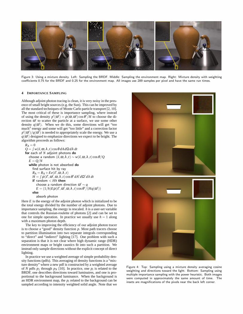
Figure 3: Using a mixture density. Left: Sampling the BRDF. Middle: Sampling the environment map. Right: Mixture density with weightingcoefficients 0.75 for the BRDF and 0.25 for the environment map. All images use 289 samples per pixel and have the same run times.

4 IMPORTANCE SAMPLING

Although adjoint photon tracing is clean, it is very noisy in the pres-ence of small bright sources (e.g. the Sun). This can be improved byall the standard techniques of Monte Carlo particle transport [2, 10].The most critical of these is importance sampling, where insteadof using the densityp′(ω ′) = ρ(ω,ω ′)cosθ ′/H to choose the di-rection ω ′ to scatter the particle at a surface, we use some otherdensityq(ω ′). When we do this, some directions will get “toomuch” energy and some will get “too little” and a correction factorp′(ω ′)/q(ω ′) is needed to appropriately scale the energy. We use aq(ω ′) designed to emphasize directions we expect to be bright. Thealgorithm proceeds as follows:

RA = 0Q =

∫w(~x,ω,λ , t)cosθ dAdΩdλ dt

for each of N adjoint photons dochoose a random (~x,ω,λ , t) ∼ w(~x,ω,λ , t)cosθ/QE = Q/Nwhile photon is not absorbed do

find surface hit by rayRA = RA +Ee(~x′,ω,λ , t)H =

∫ρ(~x′,ω ′,ω,λ , t)cosθ ′ dA′ dΩ′ dλ dt

if random < Hh thenchoose a random direction ω ′

∼ qE = (1/h)Eρ(~x′,ω ′,ω,λ , t)cosθ ′/(Hq(ω ′))

elseabsorb photon

HereE is the energy of the adjoint photon which is initialized to bethe total energy divided by the number of adjoint photons. Due toimportance sampling, the energy is rescaled.h is a user-set variablethat controls the Russian-roulette of photons [2] and can be set toone for simple operation. In practice we usually useh = 1 alongwith a maximum photon depth.

The key to improving the efficiency of our adjoint photon traceris to choose a “good” density functionp. Most path tracers chooseto partition illumination into two separate integrals correspondingto “direct” and “indirect” lighting [17]. One problem with such aseparation is that it is not clear where high dynamic range (HDR)environment maps or bright caustics fit into such a partition. Weinstead only sample directions without the explicit concept of directlighting.

In practice we use a weighted average of simple probability den-sity functions (pdfs). This averaging of density functions is a “mix-ture density” where a new pdf is constructed by a weighted averageof N pdfs p1 throughpN [10]. In practice, onepi is related to theBRDF, one describes directions toward luminaires, and one is pro-portional to the background luminance. When the background isan HDR environment map, thepi related to the background can besampled according to intensity weighted solid angle. Note that we

Figure 4: Top: Sampling using a mixture density averaging cosineweighting and directions toward the light. Bottom: Sampling usingmultiple importance sampling with the power heuristic. Both imageswere computed in approximately the same amount of time. Theinsets are magnifications of the pixels near the back left corner.

need to evaluate the values of everypi regardless of which distri-bution the sample is taken from. This matters for cases where thepi have overlapping non-zero regions (e.g. sampling the BRDF andthe environment map).

This mixture density architecture can be extended recursively.The density for BRDFs can be a mixture density of a diffuse and aspecular lobe. The density for area lights can weight nearby lightsmore heavily. A density over known caustics could weight direc-tions according to an approximation of subtended solid angle. Thisemphasizes that any improvement in the weighting coefficients,even through approximations, will be beneficial in improving ef-ficiency.

An example of the power of this mixture density importancesampling technique is shown in Figure 3. Here we use brute forceimportance sampling of the environment map and the BRDFs, us-ing models and BRDF data from Lawrence et al. [12]. In addition todealing with sampling problems, the directional sampling methodproduce a very clean code architecture.

While using mixture densities is robust, it helps little over tra-ditional path tracing for simple scenes. Figure 4 (left) shows animage with depth 6 and a mixture density sampling function thatis the average of cosine density and a density that approximatesuniform sampling toward the light, using 10,000 paths per pixel.10,000 paths per pixel is approximately ten times the paths neededfor the same level of convergence as for a conventional path tracerin our experience (and approximately five times the total ray seg-ments because no explicit shadow rays are used). So adjoint photontracing is not a good choice for simple diffuse scenes. However, thismethod pays off in the presence of complex lights or participatingmedia.

In addition to changing the density we can split adjoint photonsas long as the expected weights add to one. This allows not onlytraditional splitting [10], but also any of Veach’s multiple impor-tance sampling (MIS) techniques to be integrated into adjoint pho-ton tracing [21]. The big difference is that a sample (and thus aray) is needed for each density combined with MIS, producing abranching factor above one. This is shown for the power heuristicwith exponent 2 in the right of Figure 4 for a similar runtime to theleft figure (using about half as many screen samples to make up forthe extra branching). As can be seen, if there is an advantage overthe branchless case, it is slight. In practice we usually avoid split-ting for the sake of simplicity, but some MIS splits early in the raytree does improve convergence for some scenes.

For traditional path tracers that use direct lighting, samples aregenerated on the surface of a luminaire in order to query prop-erties of the light source. Many direct lighting computations re-quire a direction and distance for a shadow ray as well as an es-timate of the emitted radiance from the light source if the pointis unoccluded [17]. While choosing a point towards a complexreflector would be fairly straightforward, it is not clear how onewould cleanly estimate the emitted radiance when the “light” is un-occluded. Our method instead considers important directions suchas those towards light sources or a complex reflector (Figure 5) andavoids determining whether or not something is occluded.

As another simple example of this distinction, consider a glasscover over a light source. For direct lighting calculations, the glasscover occludes the light source and the computation produces ashadow. In a system without direct lighting, we will simply sendsamples towards the light source more frequently and would pro-duce the appropriate image.

Figure 5: Top: A small spherical light inside a metal parabolic reflec-tor, where the sphere itself is sampled, along with a magnification ofthe front of the taller box. Bottom: The opening of the parabolic re-flector is sampled instead of the sphere. The same number of samplesare used in each and the runtimes are approximately the same.

light

ray

medium

surface

∆s

ray∆s

Figure 6: Top ray: a traditional ray-march through a heterogeneousmedium, and at each step a shadow ray is also marched. Bottomray: an adjoint photon also steps through the medium (unless theintersection can be done analytically) and if it has an interaction withthe volume it generates a new ray only at that point.

Figure 7: At one sample per pixel each pixel either hits the mediumcompletely or is all background.

5 PARTICIPATING MEDIA

Path tracers have traditionally handled participating media by per-forming shading at many points along each ray which in turn gen-erates many visibility rays each of which requires many samplesin turn as shown for the top ray in Figure 6. For each of thensteps along the ray, an estimate of the radiance reaching that pointis computed by scattering according to a phase function, samplinglight sources or some combination of the two resulting in anO(n2)algorithm (each step generatesO(n) steps for the radiance estimateand there areO(n) steps). This is just for the single scattering.The multiple scattering is done separately. However, adjoint pho-ton tracers operate as shown for the bottom ray in Figure 6 and onlyO(n) steps are needed.

TheO(n) approach arises naturally in our framework. We treatthe participating medium as a probabilistic scatterer/absorber ratherthan as an attenuating body. An adjoint photon traveling throughthe medium will either “hit” a particle and cause its shader to beexecuted, or it will pass through the medium unaffected. Althoughthis results in more randomness for a given ray, it allows us to im-plement a volume traversal using anO(n) algorithm with the sameinterface as a surface intersection.

Not surprisingly, theO(n) approach also arises naturally fortraditional photon tracers [8] as well as for bidirectional meth-ods [11, 14]. Our approach is almost identical to the first passof photon mapping, although our single-wavelength implementa-

Figure 8: Top: Traditional ray marching, 4 samples/pixel. Bottom:New probabilistic intersection, 400 samples/pixel. These images arecomputed in approximately the same time.

tion has important simplicity and efficiency advantages for volumessuch as air that absorb or scatter different wavelengths with verydifferent probabilities without adding large correction weights. Un-like the second (visualization) pass of photon mapping, we neverengage in traditionalO(n2) single-scattering computation.

Figure 7 shows adjoint photon tracing with one sample per pixeland a ray depth of one, withq(ω ′) sampling only the luminaire(usually we run it with a mixture density defined over the hemi-sphere but for this example we hardcode the density for the singlescattering case for the purpose of comparison). This effectivelydoes direct lighting within our framework and it demonstrates theprobabilistic nature of our intersection routine: adjoint photons ei-ther hit the volume or pass through it completely. Figure 8 com-pares ray marching with our probabilistic intersection method. Notethat for 4 samples per pixel, ray marching has mostly convergedexcept for the shadow, which has variance because its samples aredistributed across the light source. Our volume shading methodruns in linear time, compared to the quadratic time required for tra-ditional ray marching. This increase in efficiency allows us to uti-lize more samples per pixel with similar computational time. Thishigher sampling density leads to lower variance in other portions ofthe scene, such as shadows.

The probability of an adjoint photon scattering is allowed to varywith wavelength. For example, in Rayleigh scattering light is scat-tered inversely proportional toλ 4. This causes blue light (shorterwavelength) to be preferentially scattered when compared to redlight (longer wavelength). With a single wavelength per adjointphoton, implementing Rayleigh scattering is straightforward (seeFigure 9).Subsurface scattering is also straightforward to model asa medium inside a dielectric boundary. An example of this is shownin Figure 10.

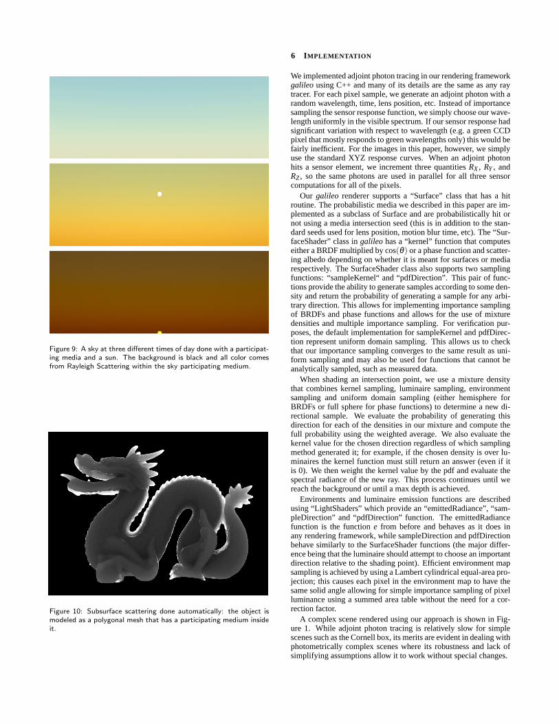
Figure 9: A sky at three different times of day done with a participat-ing media and a sun. The background is black and all color comesfrom Rayleigh Scattering within the sky participating medium.

Figure 10: Subsurface scattering done automatically: the object ismodeled as a polygonal mesh that has a participating medium insideit.

6 IMPLEMENTATION

We implemented adjoint photon tracing in our rendering frameworkgalileo using C++ and many of its details are the same as any raytracer. For each pixel sample, we generate an adjoint photon with arandom wavelength, time, lens position, etc. Instead of importancesampling the sensor response function, we simply choose our wave-length uniformly in the visible spectrum. If our sensor response hadsignificant variation with respect to wavelength (e.g. a green CCDpixel that mostly responds to green wavelengths only) this would befairly inefficient. For the images in this paper, however, we simplyuse the standard XYZ response curves. When an adjoint photonhits a sensor element, we increment three quantitiesRX , RY , andRZ , so the same photons are used in parallel for all three sensorcomputations for all of the pixels.

Our galileo renderer supports a “Surface” class that has a hitroutine. The probabilistic media we described in this paper are im-plemented as a subclass of Surface and are probabilistically hit ornot using a media intersection seed (this is in addition to the stan-dard seeds used for lens position, motion blur time, etc). The “Sur-faceShader” class ingalileo has a “kernel” function that computeseither a BRDF multiplied by cos(θ) or a phase function and scatter-ing albedo depending on whether it is meant for surfaces or mediarespectively. The SurfaceShader class also supports two samplingfunctions: “sampleKernel“ and “pdfDirection”. This pair of func-tions provide the ability to generate samples according to some den-sity and return the probability of generating a sample for any arbi-trary direction. This allows for implementing importance samplingof BRDFs and phase functions and allows for the use of mixturedensities and multiple importance sampling. For verification pur-poses, the default implementation for sampleKernel and pdfDirec-tion represent uniform domain sampling. This allows us to checkthat our importance sampling converges to the same result as uni-form sampling and may also be used for functions that cannot beanalytically sampled, such as measured data.

When shading an intersection point, we use a mixture densitythat combines kernel sampling, luminaire sampling, environmentsampling and uniform domain sampling (either hemisphere forBRDFs or full sphere for phase functions) to determine a new di-rectional sample. We evaluate the probability of generating thisdirection for each of the densities in our mixture and compute thefull probability using the weighted average. We also evaluate thekernel value for the chosen direction regardless of which samplingmethod generated it; for example, if the chosen density is over lu-minaires the kernel function must still return an answer (even if itis 0). We then weight the kernel value by the pdf and evaluate thespectral radiance of the new ray. This process continues until wereach the background or until a max depth is achieved.

Environments and luminaire emission functions are describedusing “LightShaders” which provide an “emittedRadiance”, “sam-pleDirection” and “pdfDirection” function. The emittedRadiancefunction is the functione from before and behaves as it does inany rendering framework, while sampleDirection and pdfDirectionbehave similarly to the SurfaceShader functions (the major differ-ence being that the luminaire should attempt to choose an importantdirection relative to the shading point). Efficient environment mapsampling is achieved by using a Lambert cylindrical equal-area pro-jection; this causes each pixel in the environment map to have thesame solid angle allowing for simple importance sampling of pixelluminance using a summed area table without the need for a cor-rection factor.

A complex scene rendered using our approach is shown in Fig-ure 1. While adjoint photon tracing is relatively slow for simplescenes such as the Cornell box, its merits are evident in dealing withphotometrically complex scenes where its robustness and lack ofsimplifying assumptions allow it to work without special changes.

7 DISCUSSION

Adjoint photon tracing is in some sense a rehash of neutron trans-port work from the 1940s and 1950s, and most (and possibly all) ofthe details of its implementation have appeared in different placesin the graphics literature. However, we have found that our im-plementation as a whole seems quite different and is simpler thananything we have seen in the graphics literature or encountered indiscussions with other rendering researchers. We now explicitlyaddress several questions about adjoint photon tracing.

Isn’t adjoint photon tracing just path tracing? It is simi-lar but has three important differences. First it abandons traditionaldirect lighting which fundamentally changes the architecture of apath tracer. Second it handles media differently by avoiding tra-ditional ray marching. Finally, it avoids the more complex mathof Monte Carlo integration and replaces it with Monte Carlo simu-lation. Imagine teaching both derivations to a freshman computerscience class and that advantage is quickly apparent.

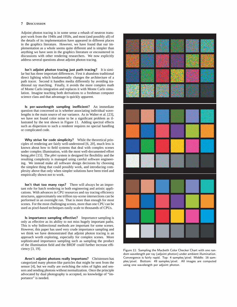
Is per-wavelength sampling inefficient? An immediatequestion that concerned us is whether associating individual wave-lengths is the main source of our variance. As in Walter et al. [23],we have not found color noise to be a significant problem as il-lustrated by the test shown in Figure 11. Adding spectral effectssuch as dispersion to such a renderer requires no special handlingor complicated code.

Why strive for code simplicity? While the theoretical prin-ciples of rendering are fairly well-understood [6, 20], much less isknown about how to field systems that deal with complex scenesunder complex illumination, with the most well-documented effortbeingpbrt [15]. Thepbrt system is designed for flexibility and theresulting complexity is managed using careful software engineer-ing. We instead make all software design decisions by choosingthe simplest thing that could possibly work, and introducing com-plexity above that only when simpler solutions have been tried andempirically shown not to work.

Isn’t that too many rays? There will always be an impor-tant role for batch rendering in both engineering and artistic appli-cations. With advances in CPU resources and ray tracing efficiencystructures, approximately one trillion ray-scene intersections can beperformed in an overnight run. That is more than enough for mostscenes. For the most challenging scenes, more than one CPU can beused as pixel-based techniques easily scale to thousands of CPUs.

Is importance sampling effective? Importance sampling isonly as effective as its ability to not miss hugely important paths.This is why bidirectional methods are important for some scenes.However, this paper has used very crude importance sampling andwe think we have demonstrated that adjoint photon tracing is anapproach worth exploring, especially for complex scenes. Moresophisticated importance sampling such as sampling the productof the illumination field and the BRDF could further increase effi-ciency [3, 19].

Aren’t adjoint photons really importons? Christensen hascategorized many photon-like particles that might be sent from thesensor [4], but we really are switching the roles of lights and sen-sors and sending photons without normalization. Once the principleadvocated by dual photography is accepted, no knowledge of “im-portance” is needed.

Figure 11: Sampling the Macbeth Color Checker Chart with one ran-dom wavelength per ray (adjoint photon) under ambient illumination.Convergence is fairly rapid. Top: 4 samples/pixel. Middle: 16 sam-ples/pixel. Bottom: 49 samples/pixel. All images are computedusing one wavelength per adjoint photon.

8 CONCLUSION

An adjoint photon tracer sends adjoint photons from the sensor el-ements into the environment and records hits at luminaires. Theimplementation of an adjoint photon tracer is straightforward, andhas the important software engineering benefit of being able to im-plement participating media as randomized surfaces. From a prac-tical standpoint this is very important because, in our experience,supporting media typically uglifies a rendering system to the pointwhere it is hard to maintain it, and in adjoint photon tracing thecomplexity associated with media is cleanly hidden. Importancesampling can be used to make adjoint photon tracing practical formany scenes, including those with spectral effects and complex par-ticipating media. At a high level, an adjoint photon tracing programoperates much like a Kajiya-style path tracer. However, in its detailsit has several advantages, and is based on a more intuitive formula-tion where the details of Monte Carlo integration are hidden in theimportance sampling rates.

ACKNOWLEDGEMENTS

David Banks suggested the term “adjoint photons”. SteveMarschner participated in helpful discussions about adjoint lighttransport. The Dragon model is courtesy of the Stanford 3D DataRepository. The data for Figure 3 was provided by Jason Lawrence(Princeton University). The smoke simulation data was providedby Kyle Hegeman (SUNY Stony Brook). This work was partiallysupported by NSF grant 03-06151 and the State of Utah Center ofExcellence Program. The second author was also supported by theBarry M. Goldwater Scholarship.

REFERENCES

[1] James Arvo. Transfer equations in global illumination. Global Illumi-nation, SIGGRAPH Conference Course Notes, 1993.

[2] James Arvo and David B. Kirk. Particle transport and image synthesis.In Proceedings of SIGGRAPH, pages 63–66, 1990.

[3] David Burke, Abhijeet Ghosh, and Wolfgang Heidrich. Bidirectionalimportance sampling for direct illumination. InRendering Techniques,pages 147–156, 2005.

[4] Per H. Christensen. Adjoints and importance in rendering: Anoverview. IEEE Transactions on Visualization and Computer Graph-ics, 9(3):329–340, 2003.

[5] Per H. Christensen, David H. Salesin, and Tony D. DeRose.A con-tinuous adjoint formulation for radiance transport. InEurographicsWorkshop on Rendering, pages 95–104, 1993.

[6] Philip Dutre, Philippe Bekaert, and Kavita Bala.Advanced GlobalIllumination. AK Peters, 2003.

[7] Henrik Wann Jensen.Realistic Image Synthesis Using Photon Map-ping. AK Peters, 2001.

[8] Henrik Wann Jensen and Per H. Christensen. Efficient simulation oflight transport in scenes with participating media using photon maps.In Proceedings of SIGGRAPH, pages 311–320, 1998.

[9] James T. Kajiya. The rendering equation. InProceedings of SIG-GRAPH, pages 143–150, 1986.

[10] Malvin H. Kalos and Paula A. Whitlock.Monte Carlo methods. Vol.1: basics. Wiley-Interscience, New York, NY, USA, 1986.

[11] Eric P. Lafortune and Yves D. Willems. Rendering participating mediawith bidirectional path tracing. InEurographics Rendering Workshop,pages 91–100, 1996.

[12] Jason Lawrence, Szymon Rusinkiewicz, and Ravi Ramamoorthi. Effi-cient brdf importance sampling using a factored representation. ACMTransactions on Graphics, 23(3):496–505, 2004.

[13] S. N. Pattanaik and S. P. Mudur. The potential equation and im-portance in illumination computations.Computer Graphics Forum,12(2):131–136, 1993.

[14] Mark Pauly, Thomas Kollig, and Alexander Keller. Metropolis lighttransport for participating media. InEurographics Workshop on Ren-dering, pages 11–22, 2000.

[15] Matt Pharr and Greg Humphreys.Physically Based Rendering. Mor-gan Kaufmann, 2004.

[16] Pradeep Sen, Billy Chen, Gaurav Garg, Stephen R. Marschner, MarkHorowitz, Marc Levoy, and Hendrik P. A. Lensch. Dual photography.ACM Transactions on Graphics, 24(3):745–755, 2005.

[17] Peter Shirley, Changyaw Wang, and Kurt Zimmerman. Monte carlotechniques for direct lighting calculations.ACM Transactions onGraphics, 15(1):1–36, January 1996.

[18] Brian E. Smits, James R. Arvo, and David H. Salesin. An importance-driven radiosity algorithm. InProceedings of SIGGRAPH, pages 273–282, 1992.

[19] Justin Talbot, David Cline, and Parris Egbert. Importance resamplingfor global illumination. InRendering Techniques, pages 139–146,2005.

[20] Eric Veach.Robust Monte Carlo Methods for Light Transport Simu-lation. PhD thesis, Stanford University, December 1997.

[21] Eric Veach and Leonidas J. Guibas. Optimally combining samplingtechniques for monte carlo rendering. InProceedings of SIGGRAPH,pages 419–428, 1995.

[22] Eric Veach and Leonidas J Guibas. Metropolis light transport. InProceedings of SIGGRAPH, pages 65–76, 1997.

[23] Bruce Walter, Philip M. Hubbard, Peter Shirley, and Donald F. Green-berg. Global illumination using local linear density estimation. ACMTransactions on Graphics, 16(3):217–259, 1997.