Image Stitching

Tamara BergCSE 590 Computational Photography

Many slides from Alyosha Efros & Derek Hoiem

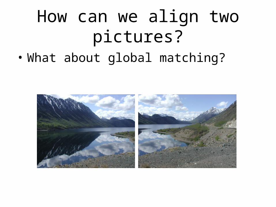
How can we align two pictures?

• What about global matching?

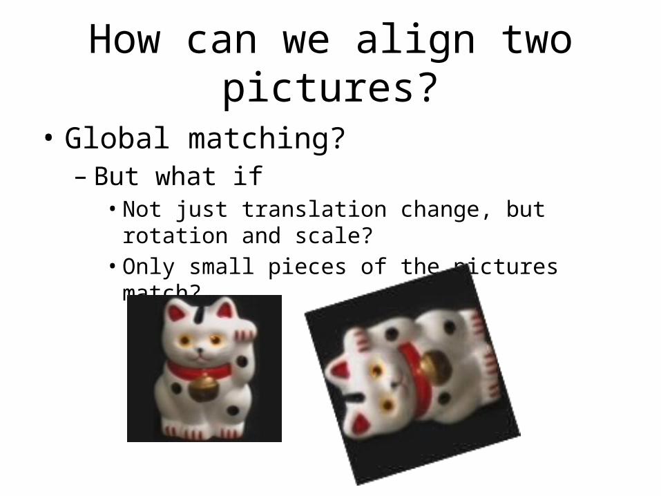
How can we align two pictures?

• Global matching?– But what if

• Not just translation change, but rotation and scale?• Only small pieces of the pictures match?

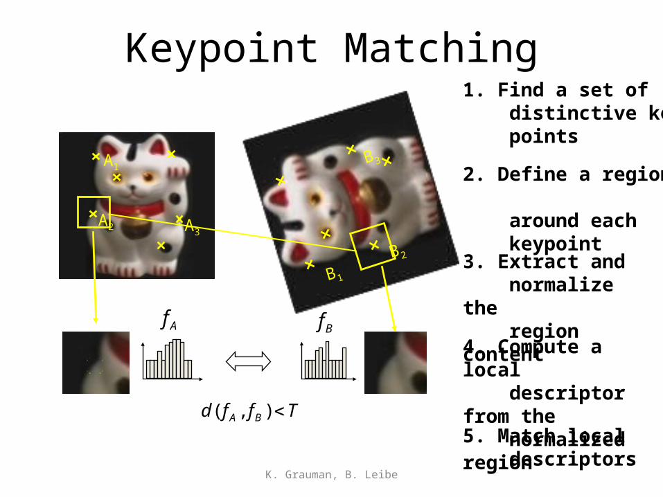
Keypoint Matching

K. Grauman, B. Leibe

Af Bf

B1

B2

B3A1

A2 A3

Tffd BA ),(

1. Find a set of distinctive key- points

3. Extract and normalize the region content

2. Define a region around each keypoint

4. Compute a local descriptor from the normalized region

5. Match local descriptors

Main challenges

• Change in position, scale, and rotation

• Change in viewpoint

• Occlusion

• Articulation, change in appearance

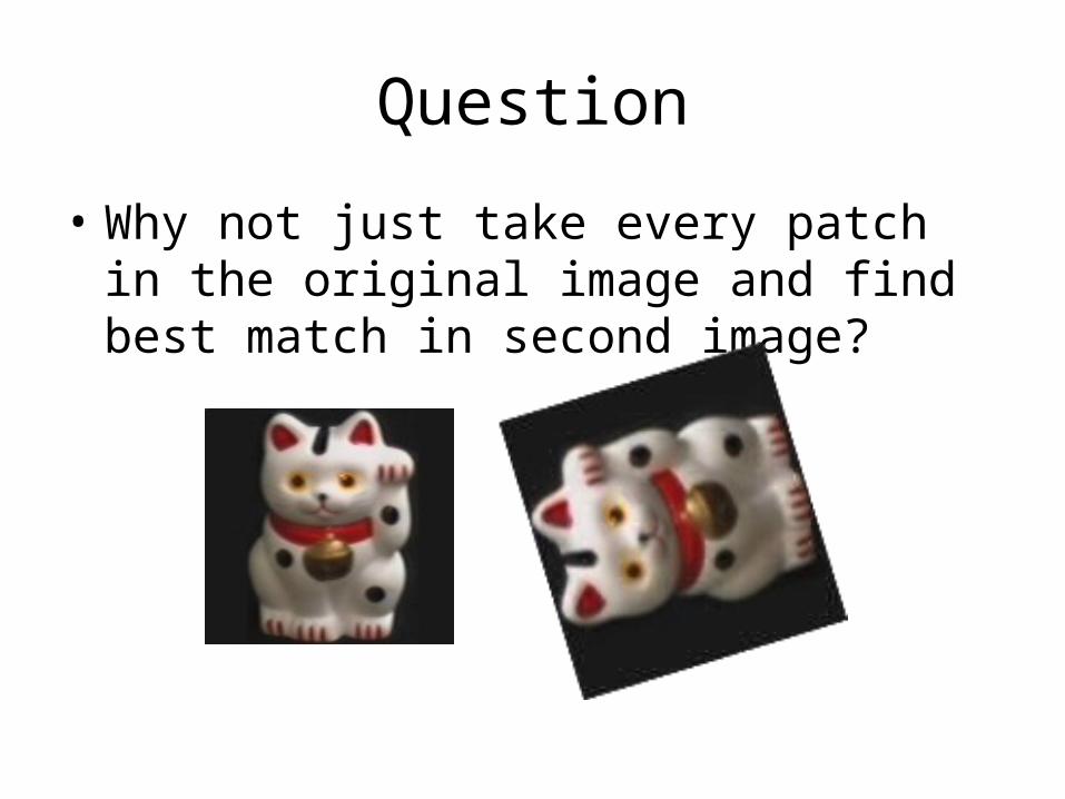
Question

• Why not just take every patch in the original image and find best match in second image?

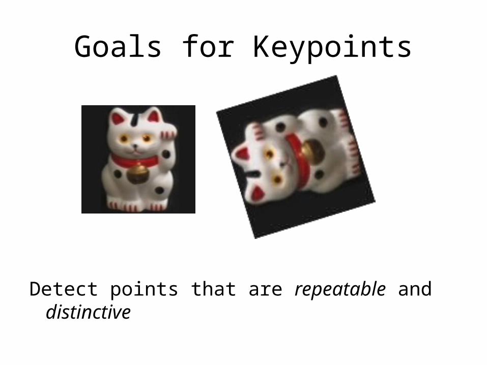
Goals for Keypoints

Detect points that are repeatable and distinctive

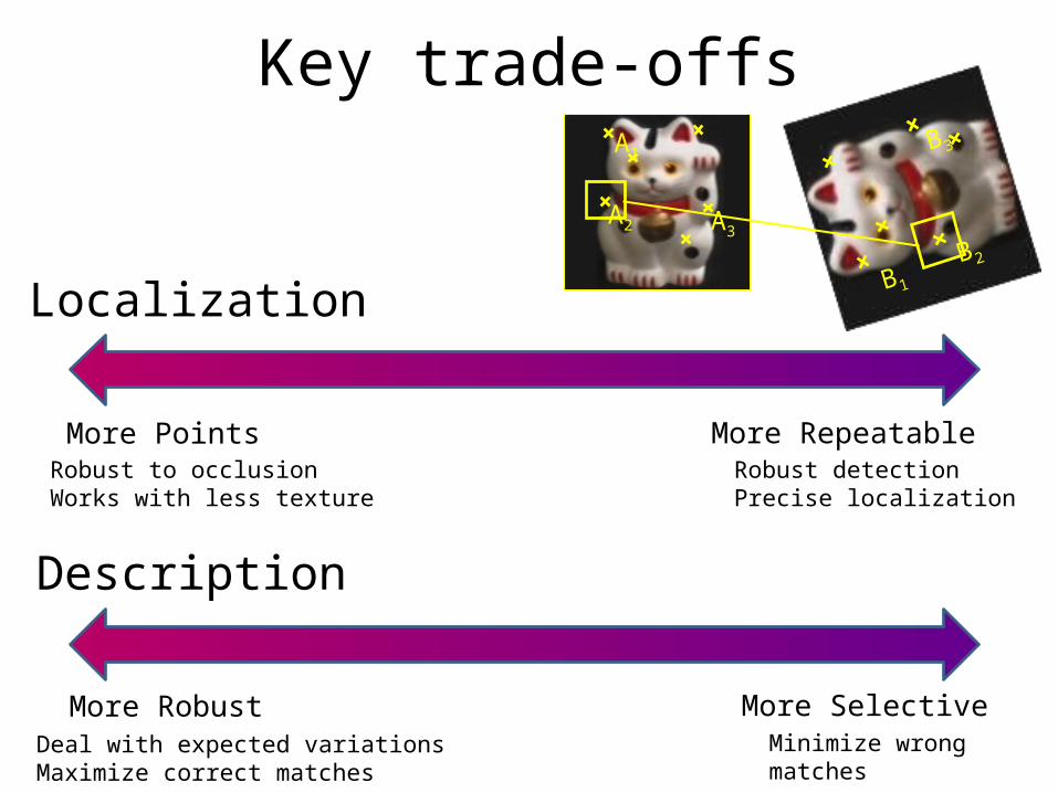
Key trade-offs

More Points More Repeatable

B1

B2

B3A1

A2 A3

Localization

More Robust More Selective

Description

Robust to occlusionWorks with less texture

Robust detectionPrecise localization

Deal with expected variationsMaximize correct matches

Minimize wrong matches

Keypoint Localization

• Goals: – Repeatable detection– Precise localization

K. Grauman, B. Leibe

Which patches are easier to match?

?

Choosing interest points

• If you wanted to meet a friend would you saya) “Let’s meet on campus.”b) “Let’s meet on Green street.”c) “Let’s meet at Green and Wright.”

• Or if you were in a secluded area:a) “Let’s meet in the Plains of Akbar.”b) “Let’s meet on the side of Mt. Doom.”c) “Let’s meet on top of Mt. Doom.”

Choosing interest points

• Corners– “Let’s meet at Green and Wright.”

• Peaks/Valleys – “Let’s meet on top of Mt. Doom.”

Many Existing Detectors Available

K. Grauman, B. Leibe

Hessian & Harris [Beaudet ‘78], [Harris ‘88]Laplacian, DoG [Lindeberg ‘98], [Lowe 1999]Harris-/Hessian-Laplace [Mikolajczyk & Schmid ‘01]Harris-/Hessian-Affine [Mikolajczyk & Schmid ‘04]EBR and IBR [Tuytelaars & Van Gool ‘04] MSER [Matas ‘02]Salient Regions [Kadir & Brady ‘01] Others…

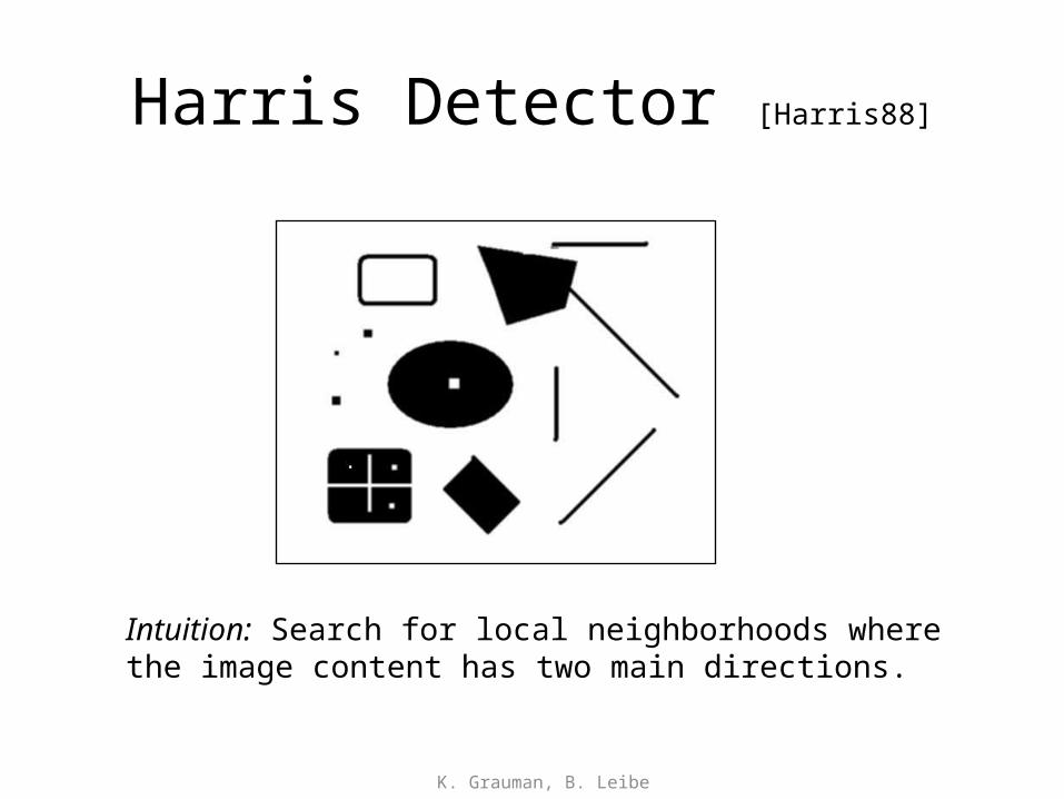
Harris Detector [Harris88]

K. Grauman, B. Leibe

Intuition: Search for local neighborhoods where the image content has two main directions.

Harris Detector – Responses [Harris88]

Effect: A very precise corner detector.

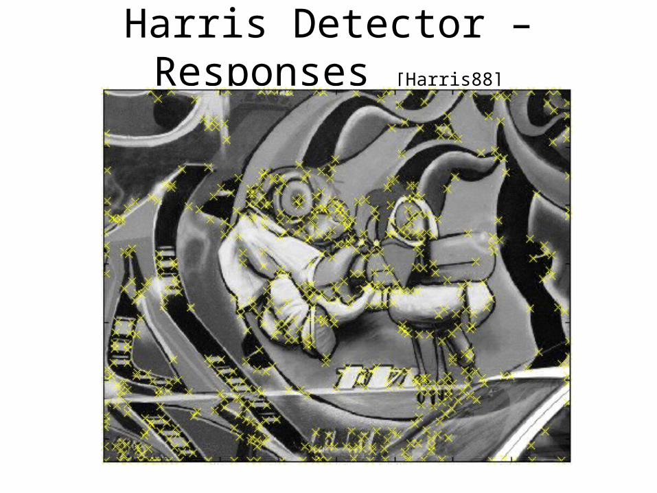
Harris Detector – Responses [Harris88]

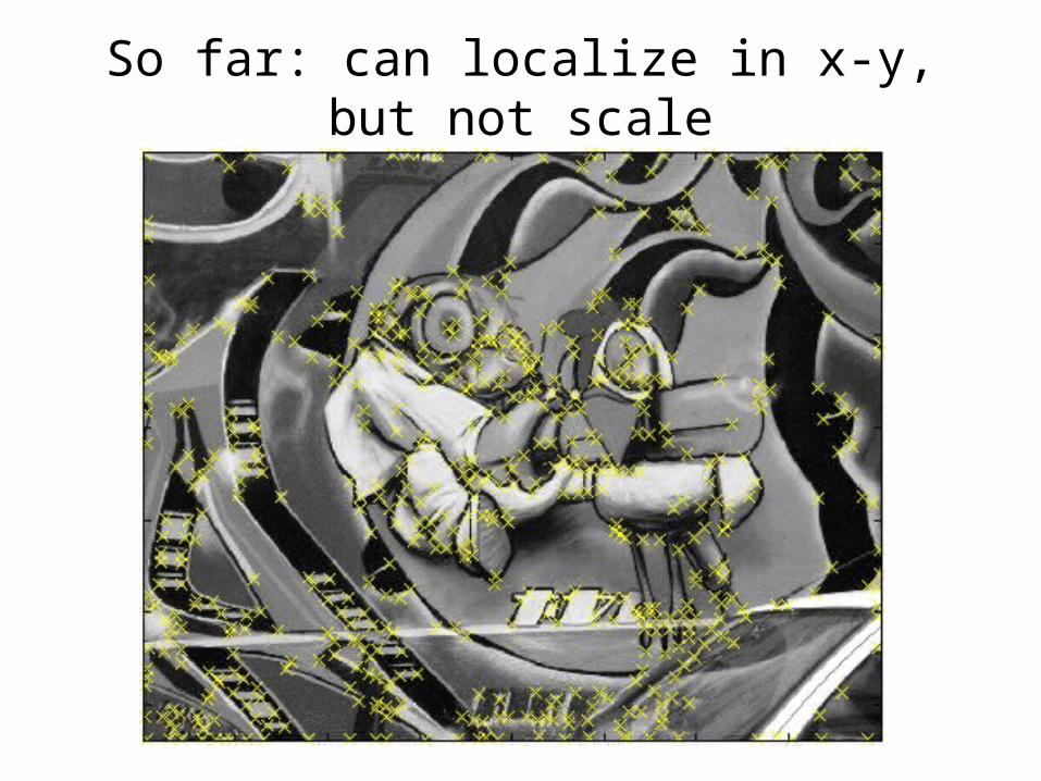
So far: can localize in x-y, but not scale

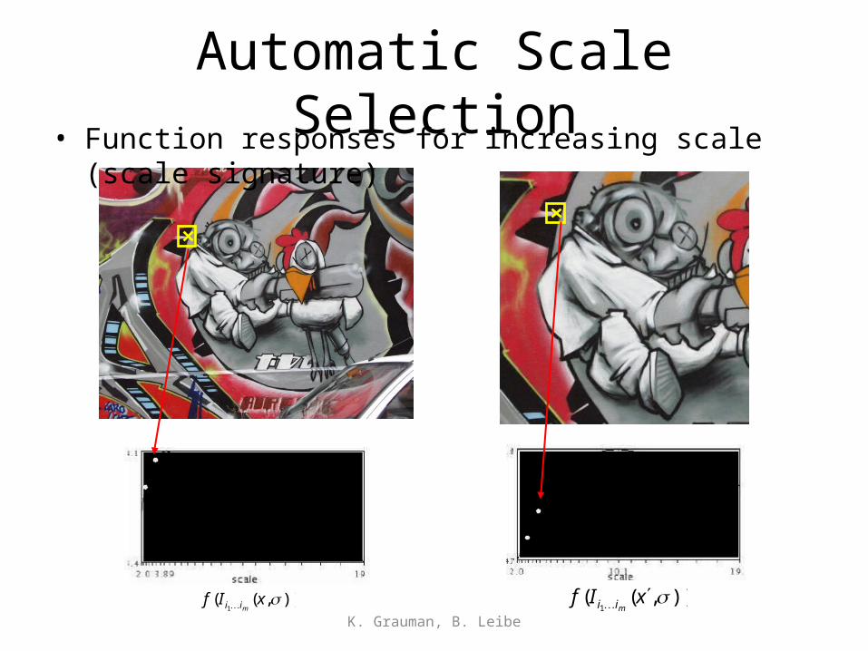
Automatic Scale Selection

K. Grauman, B. Leibe

)),(( )),((11

xIfxIfmm iiii

How to find corresponding patch sizes?

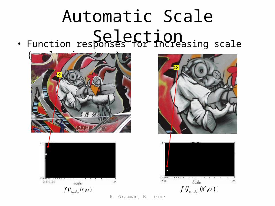
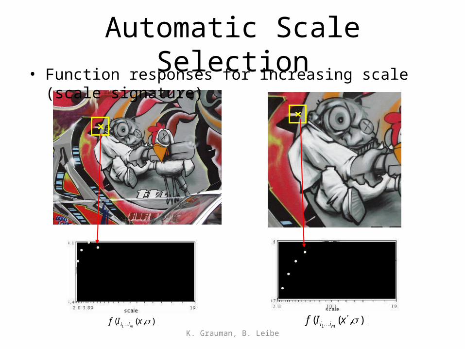
Automatic Scale Selection• Function responses for increasing scale (scale signature)

K. Grauman, B. Leibe)),((

1xIf

mii )),((1

xIfmii

Automatic Scale Selection

K. Grauman, B. Leibe)),((

1xIf

mii )),((1

xIfmii

• Function responses for increasing scale (scale signature)

Automatic Scale Selection

K. Grauman, B. Leibe)),((

1xIf

mii )),((1

xIfmii

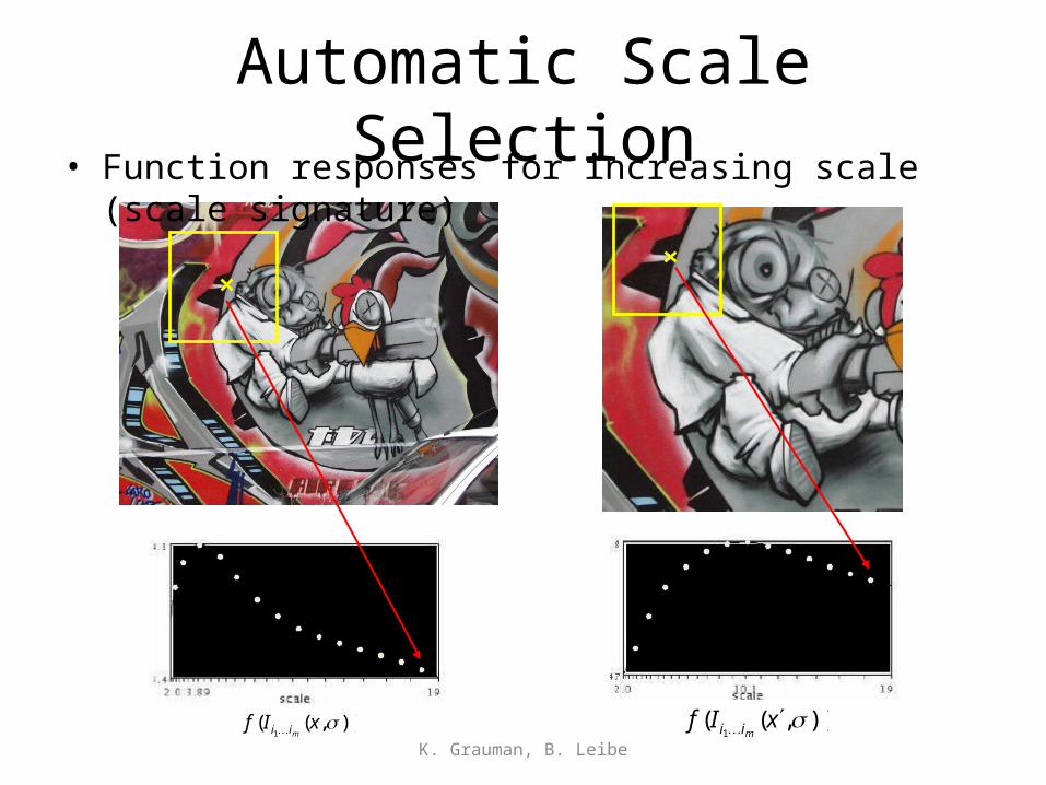
• Function responses for increasing scale (scale signature)

Automatic Scale Selection

K. Grauman, B. Leibe)),((

1xIf

mii )),((1

xIfmii

• Function responses for increasing scale (scale signature)

Automatic Scale Selection

K. Grauman, B. Leibe)),((

1xIf

mii )),((1

xIfmii

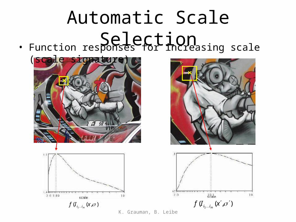
• Function responses for increasing scale (scale signature)

Automatic Scale Selection

K. Grauman, B. Leibe)),((

1xIf

mii )),((1

xIfmii

• Function responses for increasing scale (scale signature)

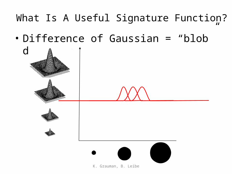
What Is A Useful Signature Function?

• Difference of Gaussian = “blob” detector

K. Grauman, B. Leibe

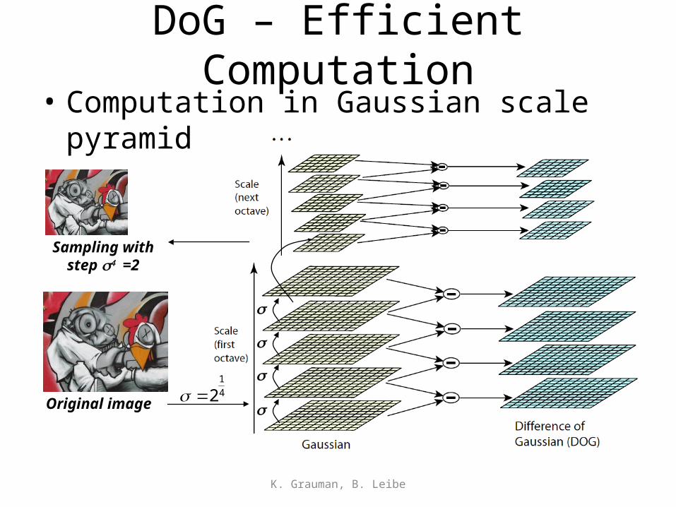
DoG – Efficient Computation• Computation in Gaussian scale pyramid

K. Grauman, B. Leibe

s

Original image 4

1

2

Sampling withstep s4 =2

s

s

s

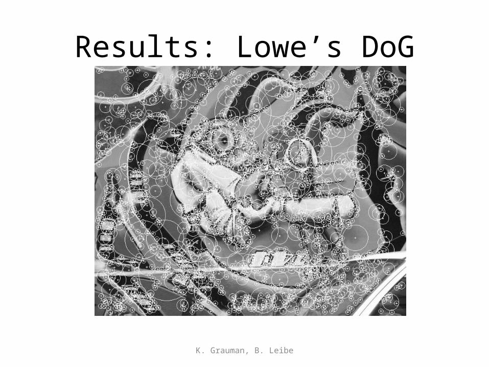
Results: Lowe’s DoG

K. Grauman, B. Leibe

T. Tuytelaars, B. Leibe

Orientation Normalization

• Compute orientation histogram• Select dominant orientation• Normalize: rotate to fixed orientation

0 2p

[Lowe, SIFT, 1999]

Available at a web site near you…

• For most local feature detectors, executables are available online:– http://robots.ox.ac.uk/~vgg/research/affine– http://www.cs.ubc.ca/~lowe/keypoints/– http://www.vision.ee.ethz.ch/~surf

K. Grauman, B. Leibe

How do we describe the keypoint?

Local Descriptors

• The ideal descriptor should be– Robust– Distinctive– Compact– Efficient

• Most available descriptors focus on edge/gradient information– Capture texture information– Color rarely used

K. Grauman, B. Leibe

Local Descriptors: SIFT Descriptor

[Lowe, ICCV 1999]

Histogram of oriented gradients

• Captures important texture information

• Robust to small translations / affine deformations

K. Grauman, B. Leibe

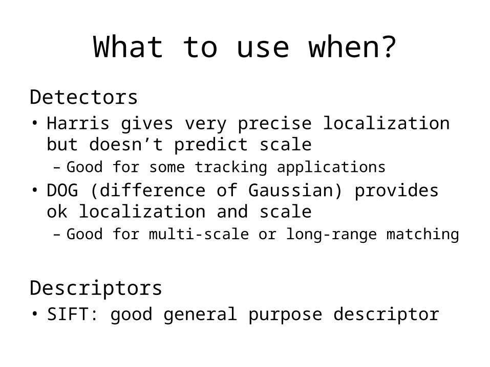
What to use when?

Detectors• Harris gives very precise localization but doesn’t

predict scale– Good for some tracking applications

• DOG (difference of Gaussian) provides ok localization and scale– Good for multi-scale or long-range matching

Descriptors• SIFT: good general purpose descriptor

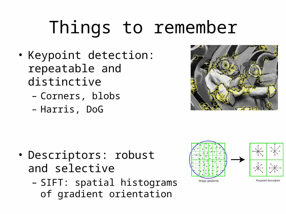
Things to remember• Keypoint detection: repeatable

and distinctive– Corners, blobs– Harris, DoG

• Descriptors: robust and selective– SIFT: spatial histograms of gradient

orientation

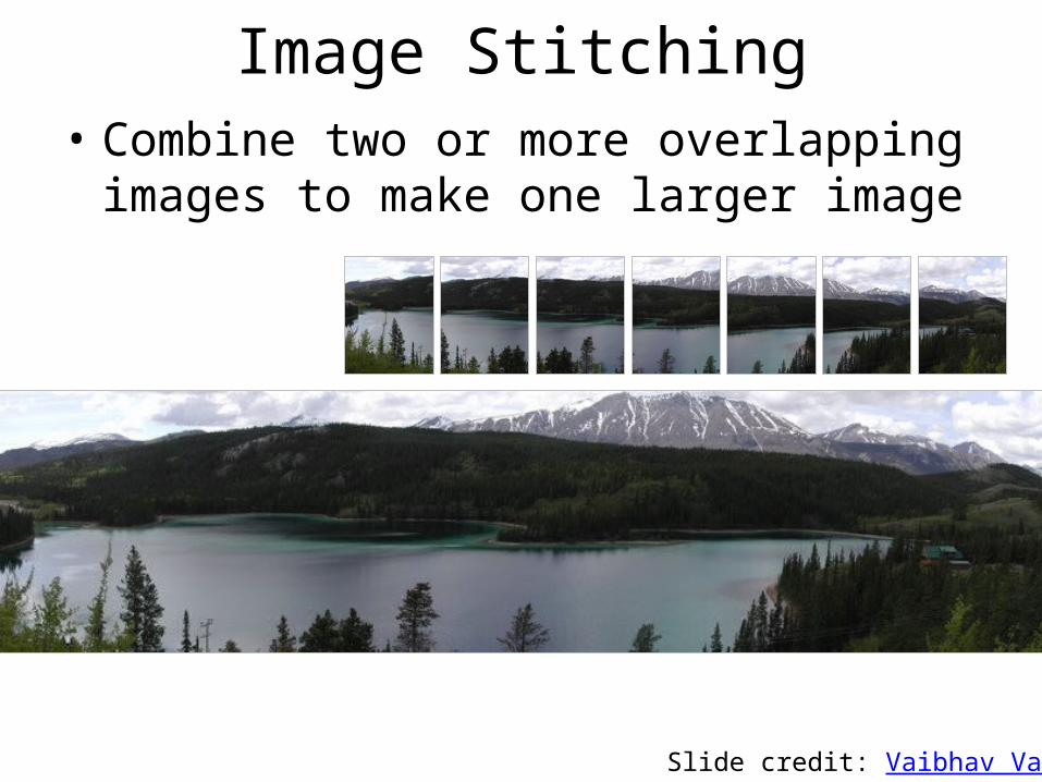
Image Stitching• Combine two or more overlapping images to

make one larger image

Add example

Slide credit: Vaibhav Vaish

Panoramic Imaging

• Higher resolution photographs, stitched from multiple images

• Capture scenes that cannot be captured in one frame

• Cheaply and easily achieve effects that used to cost a lot of money

Photo: Russell J. Hewett

Pike’s Peak Highway, CO

Nikon D70s, Tokina 12-24mm @ 16mm, f/22, 1/40s

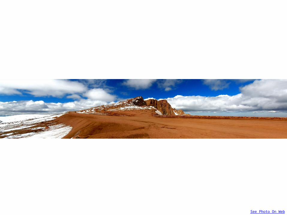
Photo: Russell J. Hewett

Pike’s Peak Highway, CO

(See Photo On Web)

Photo: Russell J. Hewett

360 Degrees, Tripod Leveled

Nikon D70, Tokina 12-24mm @ 12mm, f/8, 1/125s

Photo: Russell J. Hewett

Howth, Ireland

(See Photo On Web)

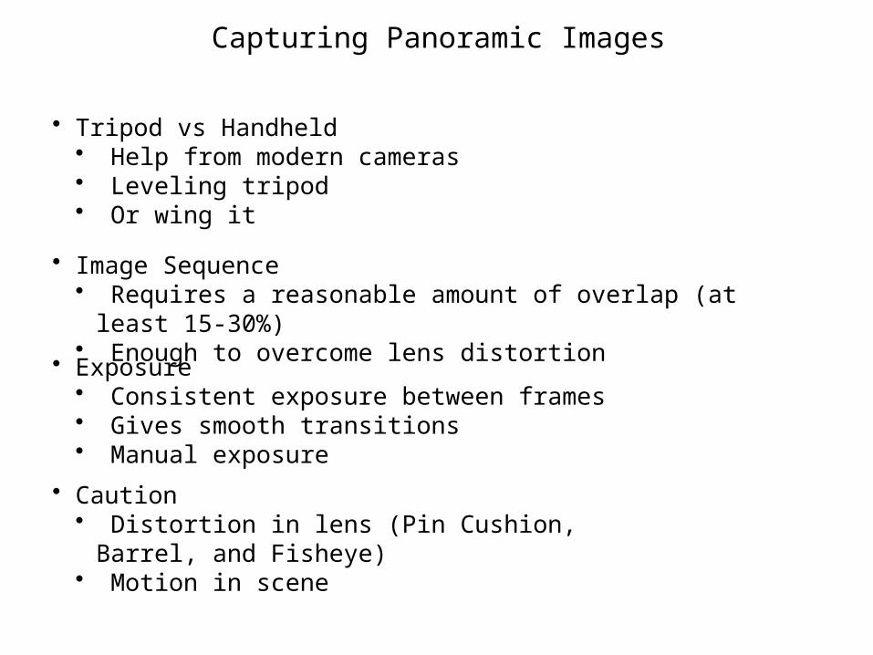
Capturing Panoramic Images

• Tripod vs Handheld• Help from modern cameras• Leveling tripod• Or wing it

• Exposure• Consistent exposure between frames• Gives smooth transitions• Manual exposure

• Caution• Distortion in lens (Pin Cushion, Barrel, and Fisheye)• Motion in scene

• Image Sequence• Requires a reasonable amount of overlap (at least 15-30%)• Enough to overcome lens distortion

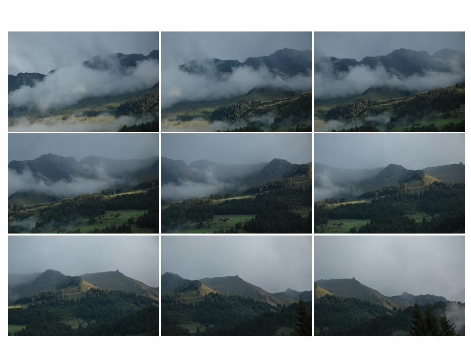
Photo: Russell J. Hewett

Handheld Camera

Nikon D70s, Nikon 18-70mm @ 70mm, f/6.3, 1/200s

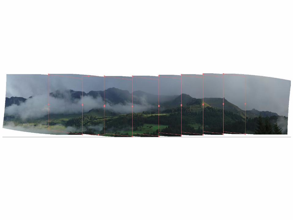
Photo: Russell J. Hewett

Handheld Camera

Photo: Russell J. Hewett

Les Diablerets, Switzerland

(See Photo On Web)

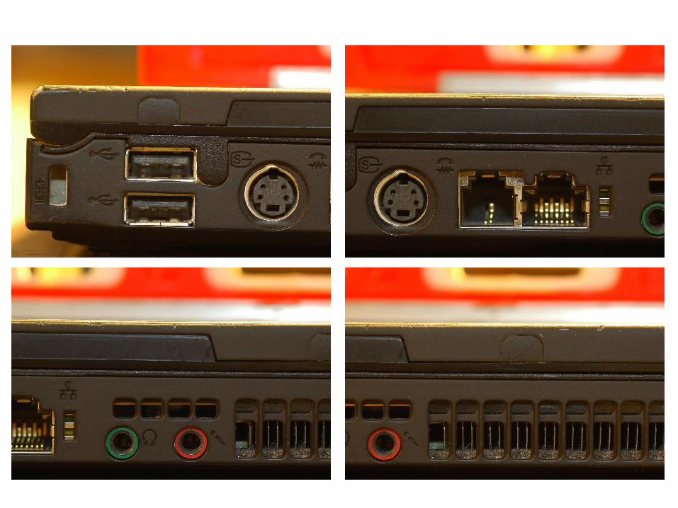
Photo: Russell J. Hewett & Bowen Lee

Macro

Nikon D70s, Tamron 90mm Micro @ 90mm, f/10, 15s

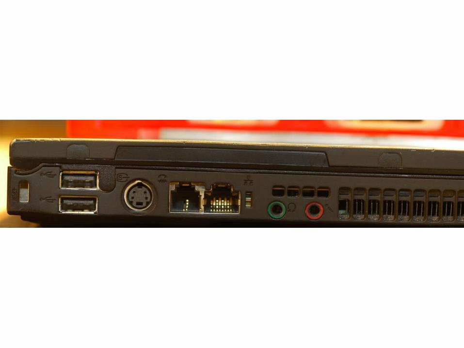
Photo: Russell J. Hewett & Bowen Lee

Side of Laptop

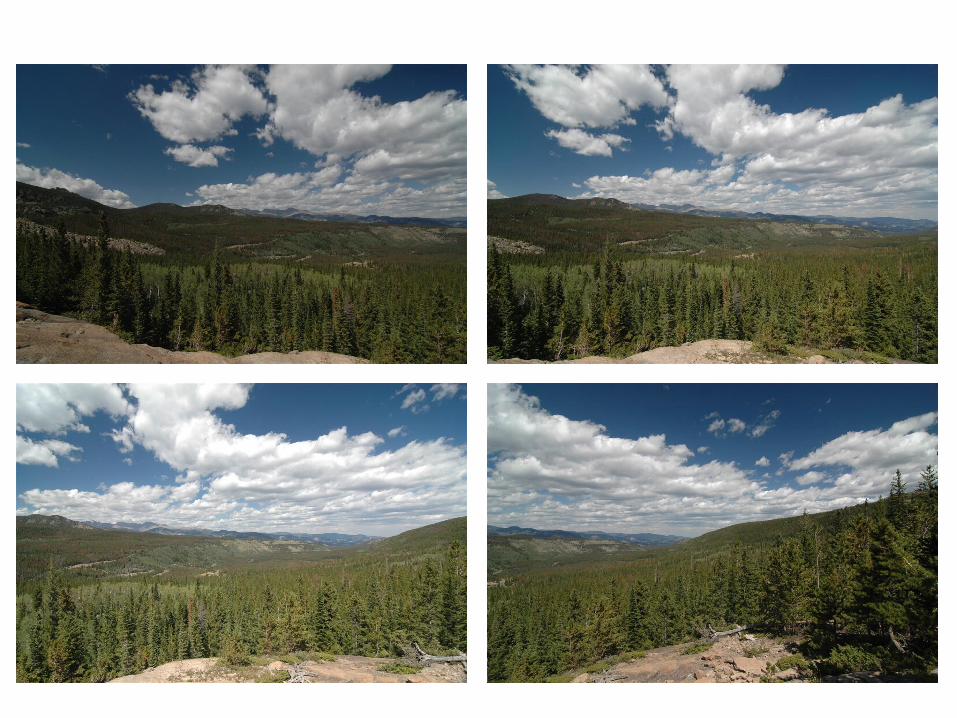
Photo: Russell J. Hewett

Ghosting and Variable Intensity

Nikon D70s, Tokina 12-24mm @ 12mm, f/8, 1/400s

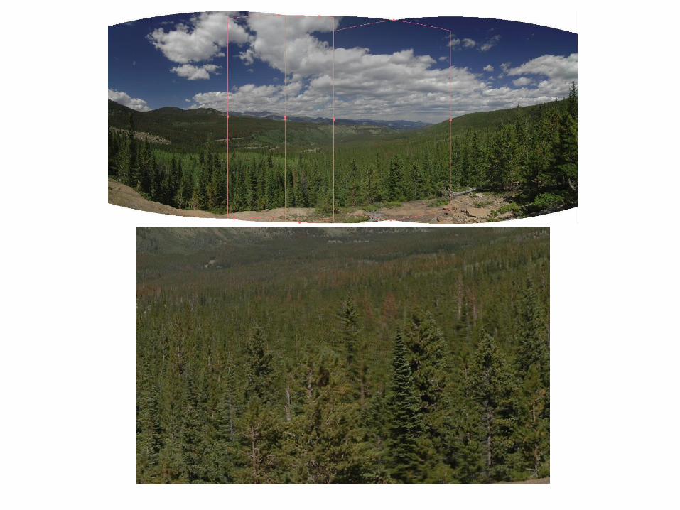
Photo: Russell J. Hewett

Photo: Bowen Lee

Ghosting From Motion

Nikon e4100 P&S

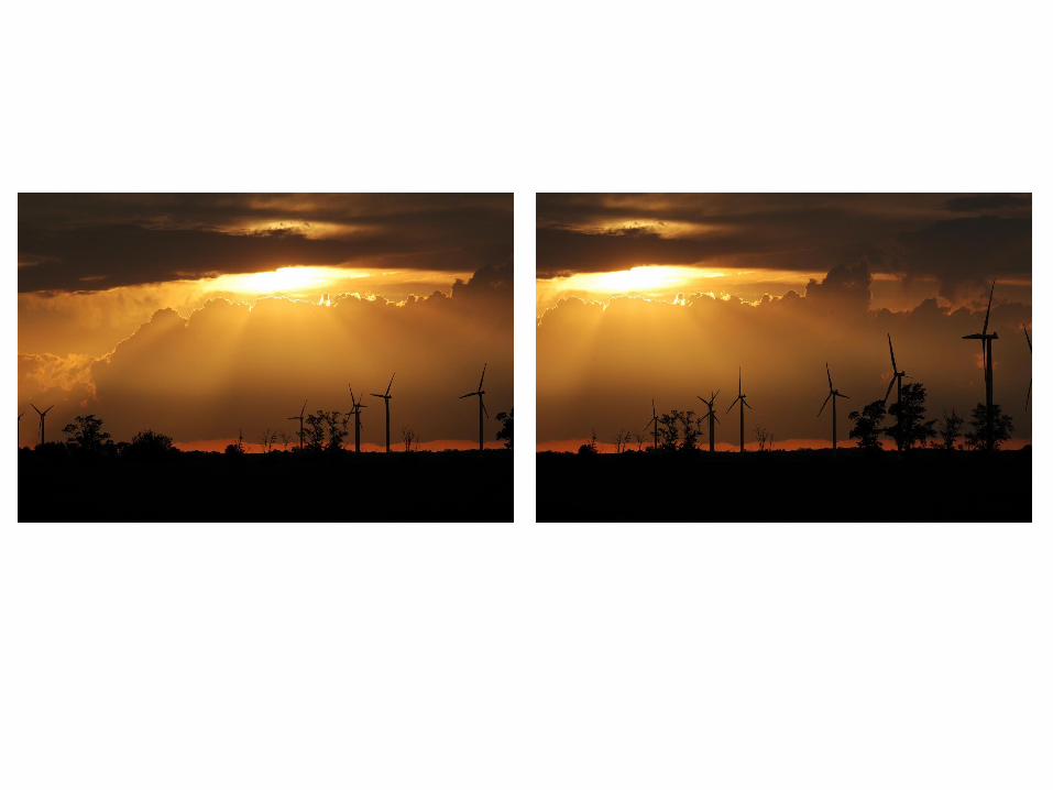
Photo: Russell J. Hewett Nikon D70, Nikon 70-210mm @ 135mm, f/11, 1/320s

Motion Between Frames

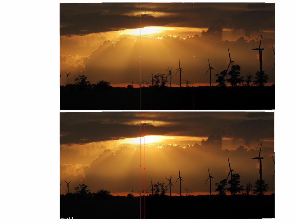
Photo: Russell J. Hewett

Photo: Russell J. Hewett

Gibson City, IL

(See Photo On Web)

Photo: Russell J. Hewett

Mount Blanca, CO

Nikon D70s, Tokina 12-24mm @ 12mm, f/22, 1/50s

Photo: Russell J. Hewett

Mount Blanca, CO

(See Photo On Web)

Image Stitching Algorithm Overview

1. Detect keypoints2. Match keypoints3. Estimate homography with matched

keypoints (using RANSAC)4. Project onto a surface and blend

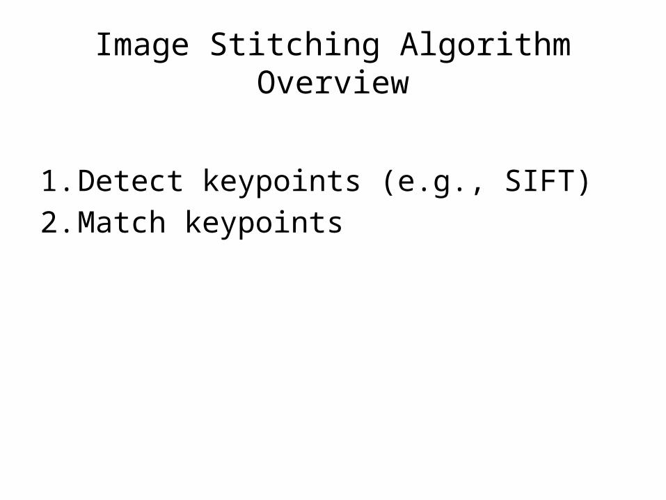
Image Stitching Algorithm Overview

1. Detect keypoints (e.g., SIFT)2. Match keypoints

Computing homography

If we have 4 matched points we can compute homography H

Hxx '

987

654

321

hhh

hhh

hhh

H

Computing homography

Assume we have matched points with outliers: How do we compute homography H?

Automatic Homography Estimation with RANSAC

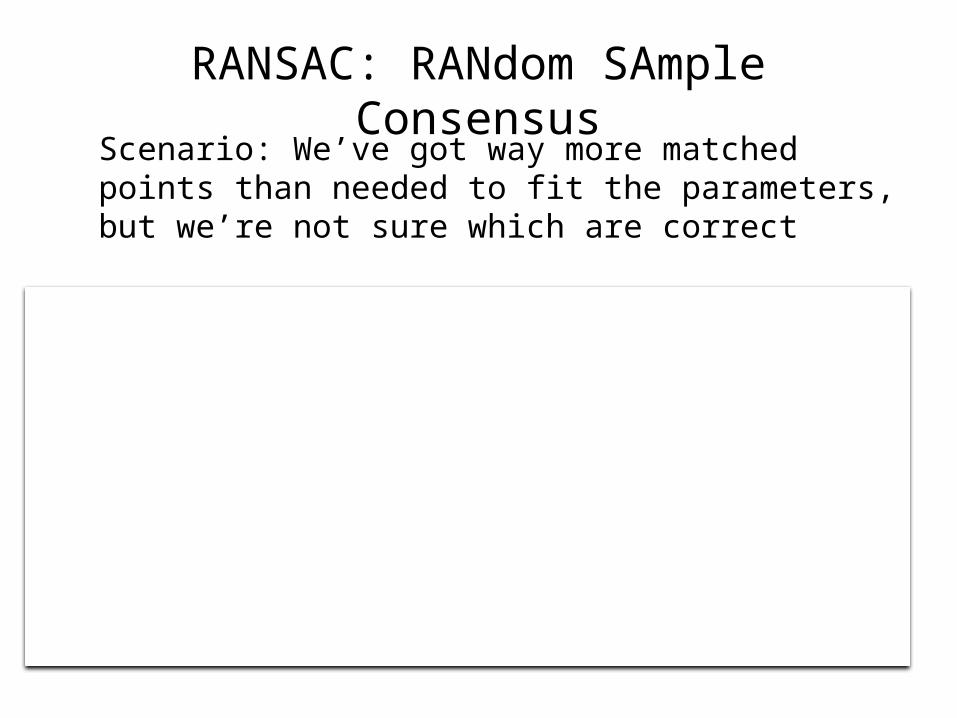
RANSAC: RANdom SAmple ConsensusScenario: We’ve got way more matched points than needed to fit the parameters, but we’re not sure which are correct

RANSAC Algorithm• Repeat N times

1. Randomly select a sample– Select just enough points to recover the parameters (4)2. Fit the model with random sample

3. See how many other points agree• Best estimate is one with most agreement

– can use agreeing points to refine estimate

Automatic Image Stitching

1. Compute interest points on each image

2. Find candidate matches

3. Estimate homography H using matched points and RANSAC

4. Project each image onto the same surface and blend

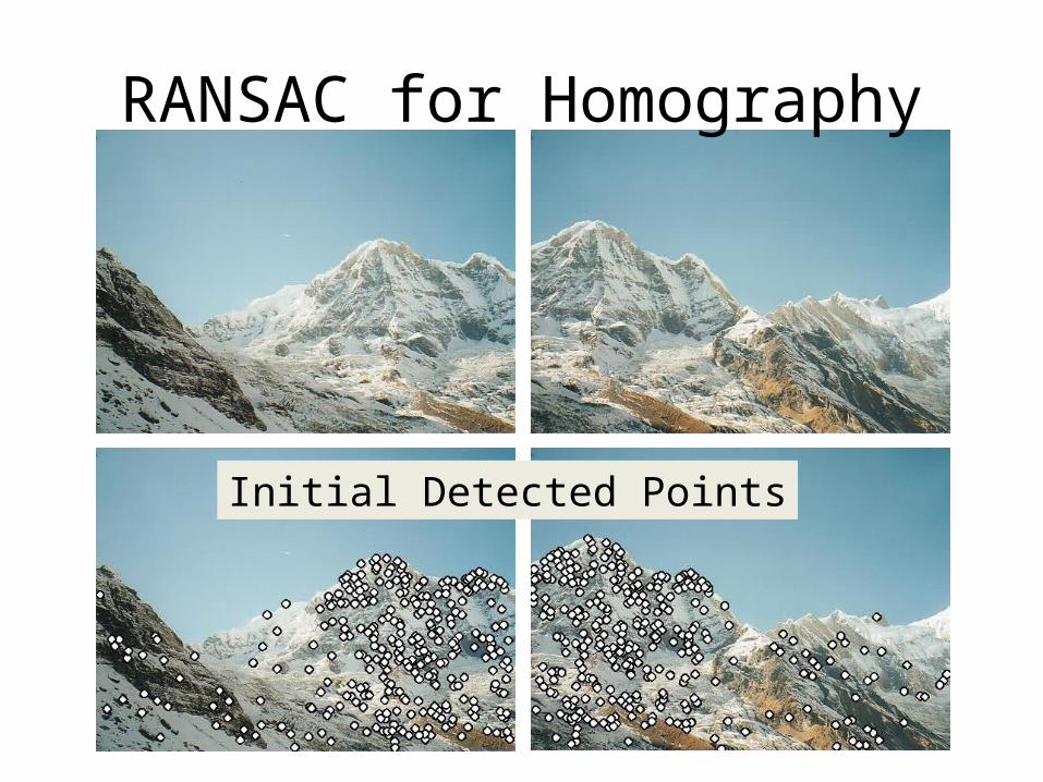
RANSAC for Homography

Initial Detected Points

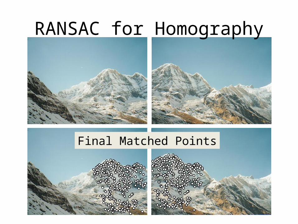
RANSAC for Homography

Final Matched Points

RANSAC for Homography

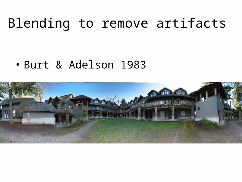
Blending to remove artifacts

• Burt & Adelson 1983

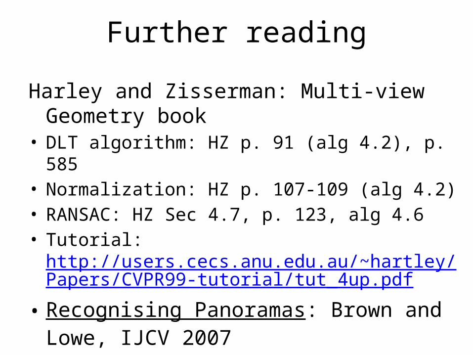
Further reading

Harley and Zisserman: Multi-view Geometry book• DLT algorithm: HZ p. 91 (alg 4.2), p. 585• Normalization: HZ p. 107-109 (alg 4.2)• RANSAC: HZ Sec 4.7, p. 123, alg 4.6• Tutorial:

http://users.cecs.anu.edu.au/~hartley/Papers/CVPR99-tutorial/tut_4up.pdf

• Recognising Panoramas: Brown and Lowe, IJCV 2007