Chapter 5

Image Segmentation

John Ashburner & Karl J. FristonThe Wellcome Dept. of Imaging Neuroscience,

12 Queen Square, London WC1N 3BG, UK.

Contents

5.1 Introduction . . . . . . . . . . . . . . . . . . . . . . . . . . . . . . . . . 1

5.2 Methods . . . . . . . . . . . . . . . . . . . . . . . . . . . . . . . . . . . . 4

5.2.1 Estimating the Cluster Parameters . . . . . . . . . . . . . . . . . . . . 5

5.2.2 Assigning Belonging Probabilities . . . . . . . . . . . . . . . . . . . . . 6

5.2.3 Estimating the Modulation Function . . . . . . . . . . . . . . . . . . 6

5.3 Examples . . . . . . . . . . . . . . . . . . . . . . . . . . . . . . . . . . . 8

5.4 Discussion . . . . . . . . . . . . . . . . . . . . . . . . . . . . . . . . . . . 11

Abstract

This chapter describes a method of segmenting MR images into different tissueclasses, using a modified Gaussian Mixture Model. By knowing the prior spatialprobability of each voxel being grey matter, white matter or cerebro-spinal fluid, itis possible to obtain a more robust classification. In addition, a step for correctingintensity non-uniformity is also included, which makes the method more applicableto images corrupted by smooth intensity variations.

5.1 Introduction

Healthy brain tissue can generally be classified into three broad tissue types on the basis of an MRimage. These are grey matter (GM), white matter (WM) and cerebro-spinal fluid (CSF). Thisclassification can be performed manually on a good quality T1 image, by simply selecting suitable

1

2 CHAPTER 5. IMAGE SEGMENTATION

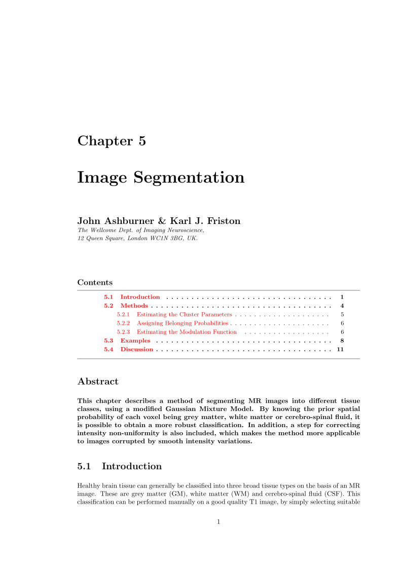
Figure 5.1: The a priori probability images of GM, WM, CSF and non-brain tissue. Values rangebetween zero (white) and one (black).

image intensity ranges which encompass most of the voxel intensities of a particular tissue type.However, this manual selection of thresholds is highly subjective.

Some groups have used clustering algorithms to partition MR images into different tissuetypes, either using images acquired from a single MR sequence, or by combining informationfrom two or more registered images acquired using different scanning sequences or echo times(eg. proton-density and T2-weighted). The approach described here is a version of the ‘mixturemodel’ clustering algorithm [8], which has been extended to include spatial maps of prior belongingprobabilities, and also a correction for image intensity non-uniformity that arises for many reasonsin MR imaging. Because the tissue classification is based on voxel intensities, partitions derivedwithout the correction can be confounded by these smooth intensity variations.

The model assumes that the MR image (or images) consists of a number of distinct tissuetypes (clusters) from which every voxel has been drawn. The intensities of voxels belonging toeach of these clusters conform to a normal distribution, which can be described by a mean, avariance and the number of voxels belonging to the distribution. For multi-spectral data (e.g.simultaneous segmentation of registered T2 and PD images), multivariate normal distributionscan be used. In addition, the model has approximate knowledge of the spatial distributions ofthese clusters, in the form of prior probability images.

Before using the current method for classifying an image, the image has to be in register withthe prior probability images. The registration is normally achieved by least squares matchingwith template images in the same stereotaxic space as the prior probability images. This can bedone using nonlinear warping, but the examples provided in this chapter were done using affineregistration (see Chapter 3).

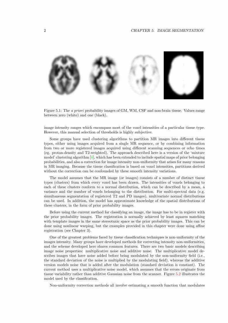
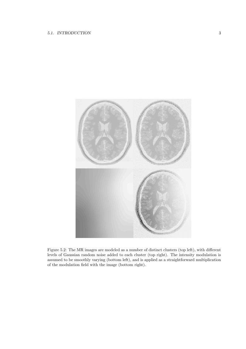
One of the greatest problems faced by tissue classification techniques is non-uniformity of theimages intensity. Many groups have developed methods for correcting intensity non-uniformities,and the scheme developed here shares common features. There are two basic models describingimage noise properties: multiplicative noise and additive noise. The multiplicative model de-scribes images that have noise added before being modulated by the non-uniformity field (i.e.,the standard deviation of the noise is multiplied by the modulating field), whereas the additiveversion models noise that is added after the modulation (standard deviation is constant). Thecurrent method uses a multiplicative noise model, which assumes that the errors originate fromtissue variability rather than additive Gaussian noise from the scanner. Figure 5.2 illustrates themodel used by the classification.

Non-uniformity correction methods all involve estimating a smooth function that modulates

5.1. INTRODUCTION 3

Figure 5.2: The MR images are modeled as a number of distinct clusters (top left), with differentlevels of Gaussian random noise added to each cluster (top right). The intensity modulation isassumed to be smoothly varying (bottom left), and is applied as a straightforward multiplicationof the modulation field with the image (bottom right).

4 CHAPTER 5. IMAGE SEGMENTATION

the image intensities. If the function is is not forced to be smooth, then it will begin to fit thehigher frequency intensity variations due to different tissue types, rather than the low frequencyintensity non-uniformity artifact. Spline [17, 13] and polynomial [14, 15] basis functions arewidely used for modeling the intensity variation. In these models, the higher frequency intensityvariations are restricted by limiting the number of basis functions. In the current method, aBayesian model is used, where it is assumed that the modulation field (U) has been drawn from apopulation for which the a priori probability distribution is known, thus allowing high frequencyvariations of the modulation field to be penalized.

5.2 Methods

The explanation of the tissue classification algorithm will be simplified by describing its applica-tion to a single two dimensional image. A number of assumptions are made by the classificationmodel. The first is that each of the I × J voxels of the image (F) has been drawn from a knownnumber (K) of distinct tissue classes (clusters). The distribution of the voxel intensities withineach class is normal (or multi-normal for multi-spectral images) and initially unknown. The dis-tribution of voxel intensities within cluster k is described by the number of voxels within thecluster (hk), the mean for that cluster (vk), and the variance around that mean (ck).

Because the images are matched to a particular stereotaxic space, prior probabilities of thevoxels belonging to the grey matter (GM), white matter (WM) and cerebro-spinal fluid (CSF)classes are known. This information is in the form of probability images – provided by theMontreal Neurological Institute [5, 4, 6] as part of the ICBM, NIH P-20 project (Principal Inves-tigator John Mazziotta), and derived from scans of 152 young healthy subjects. These probabilityimages contain values in the range of zero to one, representing the prior probability of a voxelbeing either GM, WM or CSF after an image has been normalized to the same space (see Figure5.1). The probability of a voxel at co-ordinate i, j belonging to cluster k is denoted by bijk1.

The final assumption is that the intensity and noise associated with each voxel in the imagehas been modulated by multiplication with an unknown smooth scalar field.

There are many unknown parameters to be determined by the classification algorithm, andestimating any of these requires knowledge of the others. Estimating the parameters that describea cluster (hk, vk and ck) relies on knowing which voxels belong to the cluster, and also the formof the intensity modulating function. Estimating which voxels should be assigned to each clusterrequires the cluster parameters to be defined, and also the modulation field. In turn, estimatingthe modulation field needs the cluster parameters and the belonging probabilities.

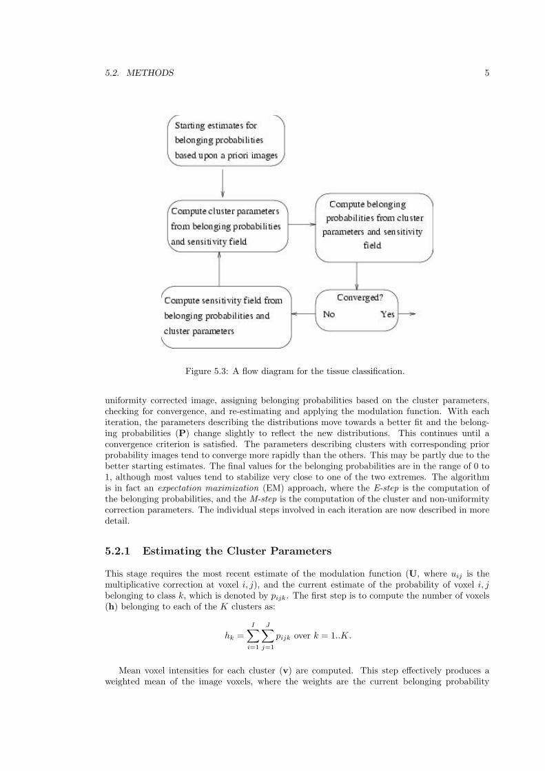
The problem requires an iterative algorithm (see Figure 5.3). It begins by assigning startingestimates for the various parameters. The starting estimate for the modulation field is typicallyuniformly one. Starting estimates for the belonging probabilities of the GM, WM and CSFpartitions are based on the prior probability images. Since there are no prior probability maps forbackground and non-brain tissue clusters, they are estimated by subtracting the prior probabilitiesfor GM, WM and CSF from a map of all ones, and dividing the result equally between theremaining clusters 2.

Each iteration of the algorithm involves estimating the cluster parameters from the non-1 Note that ij subscripts are used for voxels rather than the single subscripts used in the previous chapters.

This is to facilitate the explanation of how the modulation field is estimated for 2D images as described in Section5.2.3.

2Where identical prior probability maps are used for more than one cluster, the affected cluster parametersneed to be modified so that separate clusters can be characterised. This is typically done after the first iteration,by assigning different values for the means uniformly spaced between zero and the intensity of the white mattercluster.

5.2. METHODS 5

Figure 5.3: A flow diagram for the tissue classification.

uniformity corrected image, assigning belonging probabilities based on the cluster parameters,checking for convergence, and re-estimating and applying the modulation function. With eachiteration, the parameters describing the distributions move towards a better fit and the belong-ing probabilities (P) change slightly to reflect the new distributions. This continues until aconvergence criterion is satisfied. The parameters describing clusters with corresponding priorprobability images tend to converge more rapidly than the others. This may be partly due to thebetter starting estimates. The final values for the belonging probabilities are in the range of 0 to1, although most values tend to stabilize very close to one of the two extremes. The algorithmis in fact an expectation maximization (EM) approach, where the E-step is the computation ofthe belonging probabilities, and the M-step is the computation of the cluster and non-uniformitycorrection parameters. The individual steps involved in each iteration are now described in moredetail.

5.2.1 Estimating the Cluster Parameters

This stage requires the most recent estimate of the modulation function (U, where uij is themultiplicative correction at voxel i, j), and the current estimate of the probability of voxel i, jbelonging to class k, which is denoted by pijk. The first step is to compute the number of voxels(h) belonging to each of the K clusters as:

hk =I∑i=1

J∑j=1

pijk over k = 1..K.

Mean voxel intensities for each cluster (v) are computed. This step effectively produces aweighted mean of the image voxels, where the weights are the current belonging probability

6 CHAPTER 5. IMAGE SEGMENTATION

estimates:

vk =

∑Ii=1

∑Jj=1 pijkfijuij

hkover k = 1..K.

Then the variance of each cluster (c) is computed in a similar way to the mean:

ck =

∑Ii=1

∑Jj=1 pijk(fijuij − vk)2

hkover k = 1..K.

5.2.2 Assigning Belonging Probabilities

The next step is to re-calculate the belonging probabilities. It uses the cluster parameters com-puted in the previous step, along with the prior probability images and the intensity modulatedinput image. Bayes rule is used to assign the probability of each voxel belonging to each cluster:

pijk =rijksijk∑Kl=1 rijlsijl

over i = 1..I, j = 1..J and k = 1..K.

where pijk is the a posteriori probability that voxel i, j belongs to cluster k given its intensity offij , rijk is the likelihood of a voxel in cluster k having an intensity of fik, and sijk is the a prioriprobability of voxel i, j belonging in cluster k.

The likelihood function is obtained by evaluating the probability density functions for theclusters at each of the voxels:

rijk =uij

(2πck)1/2exp

(−(fijuij − vk)2

2ck

)over i = 1..I, j = 1..J and k = 1..K.

The prior (sijk) is based on two factors: the number of voxels currently belonging to eachcluster (hk), and the prior probability images derived from a number of images (bijk). With noknowledge of the spatial prior probability distribution of the clusters or the intensity of a voxel,then the a priori probability of any voxel belonging to a particular cluster is proportional to thenumber of voxels currently included in that cluster. However, with the additional data from theprior probability images, a better estimate for the priors can be obtained:

sijk =hkbijk∑I

l=1

∑Jm=1 blmk

over i = 1..I, j = 1..J and k = 1..K.

Convergence is ascertained by following the log-likelihood function:

I∑i=1

J∑j=1

log

(K∑k=1

rijksijk

)

The algorithm is terminated when the change in log-likelihood from the previous iteration becomesnegligible.

5.2.3 Estimating the Modulation Function

To reduce the number of parameters describing an intensity modulation field, it is modeledby a linear combination of low frequency discrete cosine transform (DCT) basis functions (see

5.2. METHODS 7

Section ??), which were chosen because there are no constraints at the boundary. A two (orthree) dimensional discrete cosine transform (DCT) is performed as a series of one dimensionaltransforms, which are simply multiplications with the DCT matrix. The elements of a matrix(D) for computing the first M coefficients of the one dimensional DCT of a vector of length I isgiven by:

di1 = 1√Ii = 1..I

dim =√

2I cos

(π(2i−1)(m−1)

2I

)i = 1..I,m = 2..M (5.1)

The matrix notation for computing the first M ×N coefficients of the two dimensional DCTof a modulation field U is Q = D1

TUD2, where the dimensions of the DCT matrices D1 andD2 are I ×M and J ×N respectively, and U is an I × J matrix. The approximate inverse DCTis computed by U ' D1QD2

T . An alternative representation of the two dimensional DCT isobtained by reshaping the I × J matrix U so that it is a vector (u). Element i+ (j − 1)× I ofthe vector is then equal to element i, j of the matrix. The two dimensional DCT can then berepresented by q = DTu, where D = D2 ⊗D1 (the Kronecker tensor product of D2 and D1),and u ' Dq.

The sensitivity correction field is computed by re-estimating the coefficients (q) of the DCTbasis functions such that the product of the likelihood and a prior probability of the parametersis increased. This can be formulated as an iteration of a Gauss-Newton optimisation algorithm(compare with Section ??):

q(n+1) =(C0−1 + A

)−1(C0−1q0 + Aq(n) − b

)(5.2)

where q0 and C0 are the means and covariance matrices describing the a priori probability distri-bution of the coefficients. Vector b contains the first derivatives of the log-likelihood cost functionwith respect to the basis function coefficients, and matrix A contains the second derivatives ofthe log-likelihood. These can be constructed efficiently using the properties of Kronecker tensorproducts (see Figure ?? in Chapter 3):

bl1 =∑Jj=1 d2jn1

∑Ii=1 d1im1

(−u−1

ij + fij∑Kk=1

pijk(fijuij−vk)ck

)Al1l2 =

∑Jj=1 d2jn1d2jn2

∑Ii=1 d1im1d1im2

(u−2ij + f2

ij

∑Kk=1

pijkck

)where l1 = m1 +M(n1 − 1) and l2 = m2 +M(n2 − 1).

Once the coefficients have been re-estimated, then the modulation field U can be computedfrom the estimated coefficients (Q) and the basis functions (D1 and D2).

uij =N∑n=1

M∑m=1

d2jnqmnd1im over i = 1..I and j = 1..J .

The Prior Probability Distribution

In Eqn. 5.2, q0 and C0 represent a multi-normal a priori probability distribution for the basisfunction coefficients. The mean of the prior probability distribution is such that it would generatea field that is uniformly one. For this, all the elements of the mean vector are set to zero, apartfrom the first element that is set to

√IJ .

The covariance matrix C0 is such that (q − q0)TC0−1(q − q0) produces an “energy” term

that penalizes modulation fields that would be unlikely a priori. There are many possible forms

8 CHAPTER 5. IMAGE SEGMENTATION

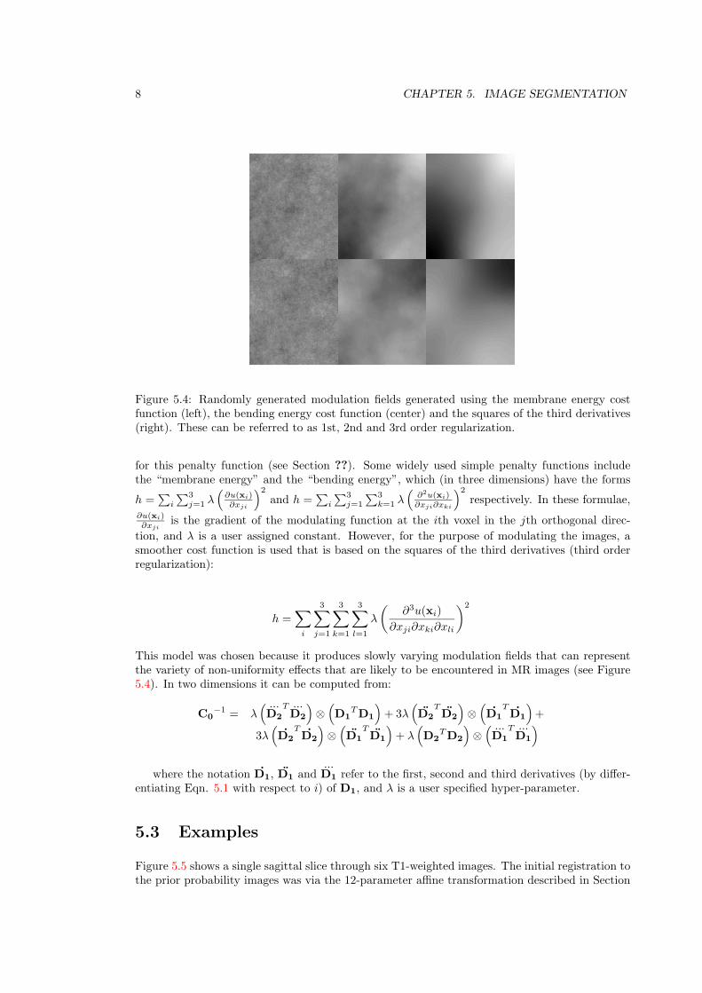
Figure 5.4: Randomly generated modulation fields generated using the membrane energy costfunction (left), the bending energy cost function (center) and the squares of the third derivatives(right). These can be referred to as 1st, 2nd and 3rd order regularization.

for this penalty function (see Section ??). Some widely used simple penalty functions includethe “membrane energy” and the “bending energy”, which (in three dimensions) have the forms

h =∑i

∑3j=1 λ

(∂u(xi)∂xji

)2

and h =∑i

∑3j=1

∑3k=1 λ

(∂2u(xi)∂xji∂xki

)2

respectively. In these formulae,∂u(xi)∂xji

is the gradient of the modulating function at the ith voxel in the jth orthogonal direc-tion, and λ is a user assigned constant. However, for the purpose of modulating the images, asmoother cost function is used that is based on the squares of the third derivatives (third orderregularization):

h =∑i

3∑j=1

3∑k=1

3∑l=1

λ

(∂3u(xi)

∂xji∂xki∂xli

)2

This model was chosen because it produces slowly varying modulation fields that can representthe variety of non-uniformity effects that are likely to be encountered in MR images (see Figure5.4). In two dimensions it can be computed from:

C0−1 = λ

( ...D2

T ...D2

)⊗(D1

TD1

)+ 3λ

(D2

TD2

)⊗(D1

TD1

)+

3λ(D2

TD2

)⊗(D1

TD1

)+ λ

(D2

TD2

)⊗( ...D1

T ...D1

)where the notation D1, D1 and

...D1 refer to the first, second and third derivatives (by differ-

entiating Eqn. 5.1 with respect to i) of D1, and λ is a user specified hyper-parameter.

5.3 Examples

Figure 5.5 shows a single sagittal slice through six T1-weighted images. The initial registration tothe prior probability images was via the 12-parameter affine transformation described in Section

5.3. EXAMPLES 9

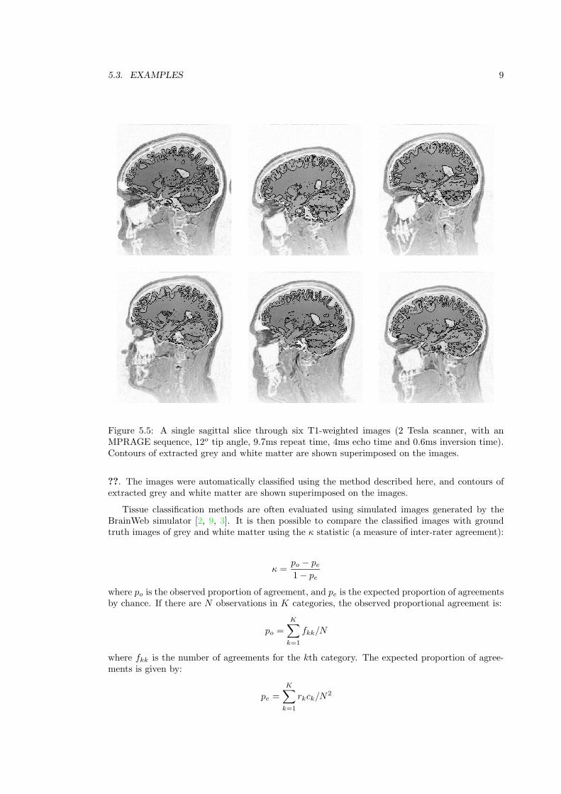
Figure 5.5: A single sagittal slice through six T1-weighted images (2 Tesla scanner, with anMPRAGE sequence, 12o tip angle, 9.7ms repeat time, 4ms echo time and 0.6ms inversion time).Contours of extracted grey and white matter are shown superimposed on the images.

??. The images were automatically classified using the method described here, and contours ofextracted grey and white matter are shown superimposed on the images.

Tissue classification methods are often evaluated using simulated images generated by theBrainWeb simulator [2, 9, 3]. It is then possible to compare the classified images with groundtruth images of grey and white matter using the κ statistic (a measure of inter-rater agreement):

κ =po − pe1− pe

where po is the observed proportion of agreement, and pe is the expected proportion of agreementsby chance. If there are N observations in K categories, the observed proportional agreement is:

po =K∑k=1

fkk/N

where fkk is the number of agreements for the kth category. The expected proportion of agree-ments is given by:

pe =K∑k=1

rkck/N2

10 CHAPTER 5. IMAGE SEGMENTATION

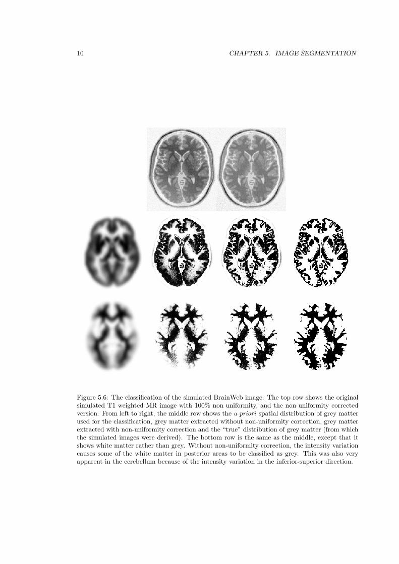
Figure 5.6: The classification of the simulated BrainWeb image. The top row shows the originalsimulated T1-weighted MR image with 100% non-uniformity, and the non-uniformity correctedversion. From left to right, the middle row shows the a priori spatial distribution of grey matterused for the classification, grey matter extracted without non-uniformity correction, grey matterextracted with non-uniformity correction and the “true” distribution of grey matter (from whichthe simulated images were derived). The bottom row is the same as the middle, except that itshows white matter rather than grey. Without non-uniformity correction, the intensity variationcauses some of the white matter in posterior areas to be classified as grey. This was also veryapparent in the cerebellum because of the intensity variation in the inferior-superior direction.

5.4. DISCUSSION 11

where rk and ck are the total number of voxels in the kth class for both the “true” and estimatedpartitions.

The classification of a single plane of the simulated T1 weighted BrainWeb image with 100%non-uniformity is illustrated in Figure 5.6. It should be noted that no pre-processing to removescalp or other non-brain tissue was performed on the image. In theory, the tissue classificationmethod should produce slightly better results if this non-brain tissue is excluded from the compu-tations. As the algorithm stands, a small amount of non-brain tissue remains in the grey matterpartition, which has arisen from voxels that lie close to grey matter and have similar intensities.

5.4 Discussion

The current segmentation method is fairly robust and accurate for high quality T1 weighted im-ages, but is not beyond improvement. Currently, each voxel is assigned a probability of belongingto a particular tissue class based only on its intensity and information from the prior probabilityimages. There is a great deal of other knowledge that could be incorporated into the classifi-cation. For example, if all a voxel’s neighbors are grey matter, then there is a high probabilitythat it should also be grey matter. Other researchers have successfully used Markov random fieldmodels to include this information in a tissue classification model [17, 16, 15, 11, 18]. Anothervery simple prior, that can be incorporated, is the relative intensity of the different tissue types[7]. For example, when segmenting a T1 weighted image, it is known that the white matter shouldhave a higher intensity than the grey matter, which in turn should be more intense than the CSF.When computing the means for each cluster, this prior information could sensibly be used to biasthe estimates.

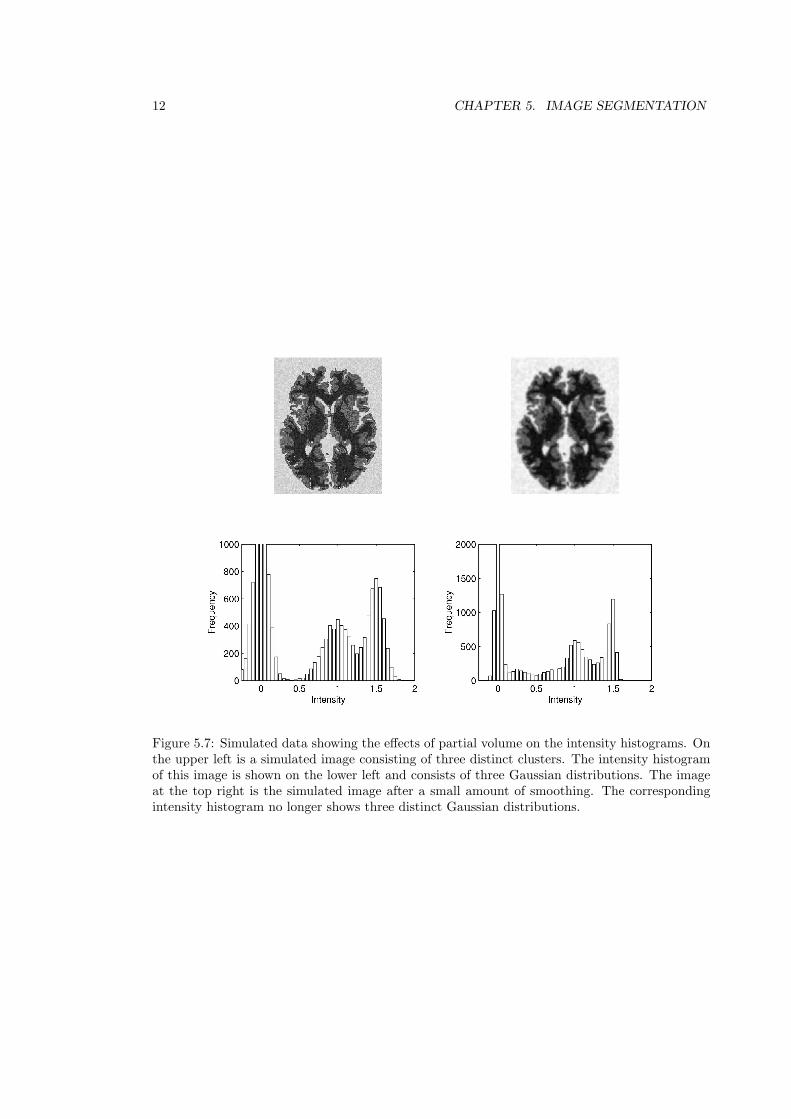
In order to function properly, the classification method requires good contrast between thedifferent tissue types. However, many central grey matter structures have image intensities thatare almost indistinguishable from that of white matter, so the tissue classification is not alwaysvery accurate in these regions. Another related problem is that of partial volume. Because themodel assumes that all voxels contain only one tissue type, the voxels that contain a mixture oftissues may not be modeled correctly. In particular, those voxels at the interface between whitematter and ventricles will often appear as grey matter. This can be seen to a small extent inFigures 5.5 and 5.6. Each voxel is assumed to be of only one tissue type, and not a combinationof different tissues, so the model’s assumptions are violated when voxels contain signal from morethan one tissue type. This problem is greatest when the voxel dimensions are large, or if theimages have been smoothed, and is illustrated using simulated data in Figure 5.7. The effectof partial volume is that it causes the distributions of the intensities to deviate from normal.Some authors have developed more complex models than mixtures of Gaussians to describe theintensity distributions of the classes [1]. A more recent commonly adopted approach involvesmodeling separate classes of partial volumed voxels [10, 11, 12].

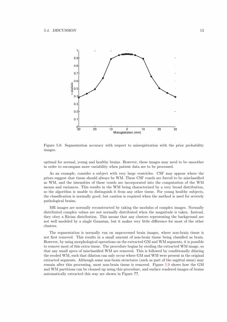
In order for the Bayesian classification to work properly, an image volume must be in registerwith a set of prior probability images used to instate the priors. Figure 5.8 shows the effects ofmis-registration on the accuracy of segmentation. This figure also gives an indication of how fara brain can deviate from the normal population of brains (that constitute the prior probabilityimages) in order for it to be segmented adequately. Clearly, if the brain cannot be well registeredwith the probability images, then the segmentation will not be as accurate. This fact also hasimplications for severely abnormal brains, as they are more difficult to register with images thatrepresent the prior probabilities of voxels belonging to different classes. Segmenting such abnormalbrains can be a problem for the algorithm, as the prior probability images are based on normalhealthy brains. The profile in Figure 5.8 depends on the smoothness or resolution of the priorprobability images. By not smoothing the prior probability images, the segmentation would be

12 CHAPTER 5. IMAGE SEGMENTATION

Figure 5.7: Simulated data showing the effects of partial volume on the intensity histograms. Onthe upper left is a simulated image consisting of three distinct clusters. The intensity histogramof this image is shown on the lower left and consists of three Gaussian distributions. The imageat the top right is the simulated image after a small amount of smoothing. The correspondingintensity histogram no longer shows three distinct Gaussian distributions.

5.4. DISCUSSION 13

Figure 5.8: Segmentation accuracy with respect to misregistration with the prior probabilityimages.

optimal for normal, young and healthy brains. However, these images may need to be smootherin order to encompass more variability when patient data are to be processed.

As an example, consider a subject with very large ventricles. CSF may appear where thepriors suggest that tissue should always be WM. These CSF voxels are forced to be misclassifiedas WM, and the intensities of these voxels are incorporated into the computation of the WMmeans and variances. This results in the WM being characterized by a very broad distribution,so the algorithm is unable to distinguish it from any other tissue. For young healthy subjects,the classification is normally good, but caution is required when the method is used for severelypathological brains.

MR images are normally reconstructed by taking the modulus of complex images. Normallydistributed complex values are not normally distributed when the magnitude is taken. Instead,they obey a Rician distribution. This means that any clusters representing the background arenot well modeled by a single Gaussian, but it makes very little difference for most of the otherclusters.

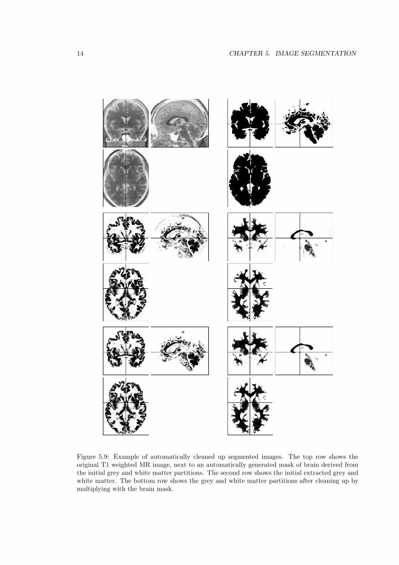
The segmentation is normally run on unprocessed brain images, where non-brain tissue isnot first removed. This results in a small amount of non-brain tissue being classified as brain.However, by using morphological operations on the extracted GM and WM segments, it is possibleto remove most of this extra tissue. The procedure begins by eroding the extracted WM image, sothat any small specs of misclassified WM are removed. This is followed by conditionally dilatingthe eroded WM, such that dilation can only occur where GM and WM were present in the originalextracted segments. Although some non-brain structures (such as part of the sagittal sinus) mayremain after this processing, most non-brain tissue is removed. Figure 5.9 shows how the GMand WM partitions can be cleaned up using this procedure, and surface rendered images of brainsautomatically extracted this way are shown in Figure ??.

14 CHAPTER 5. IMAGE SEGMENTATION

Figure 5.9: Example of automatically cleaned up segmented images. The top row shows theoriginal T1 weighted MR image, next to an automatically generated mask of brain derived fromthe initial grey and white matter partitions. The second row shows the initial extracted grey andwhite matter. The bottom row shows the grey and white matter partitions after cleaning up bymultiplying with the brain mask.

BIBLIOGRAPHY 15

Bibliography

[1] E. Bullmore, M. Brammer, G. Rouleau, B. Everitt, A. Simmons, T. Sharma, S. Frangou,R. Murray, and G. Dunn. Computerized brain tissue classification of magnetic resonanceimages: A new approach to the problem of partial volume artifact. NeuroImage, 2:133–147,1995.

[2] C.A. Cocosco, V. Kollokian, R.K.-S. Kwan, and A.C. Evans. Brainweb: Online interface toa 3D MRI simulated brain database. NeuroImage, 5(4):S425, 1997.

[3] D.L. Collins, A.P. Zijdenbos, V. Kollokian, J.G. Sled, N.J. Kabani, C.J. Holmes, and A.C.Evans. Design and construction of a realistic digital brain phantom. IEEE Transactions onMedical Imaging, 17(3):463–468, 1998.

[4] A. C. Evans, D. L. Collins, S. R. Mills, E. D. Brown, R. L. Kelly, and T. M. Peters. 3Dstatistical neuroanatomical models from 305 MRI volumes. In Proc. IEEE-Nuclear ScienceSymposium and Medical Imaging Conference, pages 1813–1817, 1993.

[5] A. C. Evans, D. L. Collins, and B. Milner. An MRI-based stereotactic atlas from 250 youngnormal subjects. Society of Neuroscience Abstracts, 18:408, 1992.

[6] A. C. Evans, M. Kamber, D. L. Collins, and D. Macdonald. An MRI-based probabilisticatlas of neuroanatomy. In S. Shorvon, D. Fish, F. Andermann, G. M. Bydder, and StefanH, editors, Magnetic Resonance Scanning and Epilepsy, volume 264 of NATO ASI Series A,Life Sciences, pages 263–274. Plenum Press, 1994.

[7] B. Fischl, D. H. Salat, E. Busa, M. Albert, M. Dieterich, C. Haselgrove, A. van der Kouwe,R. Killiany, D. Kennedy, S. Klaveness, A. Montillo, N. Makris, B. Rosen, and A. M. Dale.Whole brain segmentation: Automated labeling of neuroanatomical structures in the humanbrain. Neuron, 33:341–355, 2002.

[8] J. A. Hartigan. Clustering Algorithms, pages 113–129. John Wiley & Sons, Inc., New York,1975.

[9] R. K.-S. Kwan, A. C. Evans, and G. B. Pike. An extensible MRI simulator for post-processingevaluation. In Proc. Visualization in Biomedical Computing, pages 135–140, 1996.

[10] D. H. Laidlaw, K. W. Fleischer, and A. H. Barr. Partial-volume bayesian classification ofmaterial mixtures in MR volume data using voxel histograms. IEEE Transactions on MedicalImaging, 17(1):74–86, 1998.

[11] S. Ruan, C. Jaggi, J. Xue, J. Fadili, and D. Bloyet. Brain tissue classification of magneticresonance images using partial volume modeling. IEEE Transactions on Medical Imaging,19(12):1179–1187, 2000.

[12] D. W. Shattuck, S. R. Sandor-Leahy, K. A. Schaper, D. A. Rottenberg, and R. M. Leahy.Magnetic resonance image tissue classification using a partial volume model. NeuroImage,13(5):856–876, 2001.

[13] J. G. Sled, A. P. Zijdenbos, and A. C. Evans. A non-parametric method for automaticcorrection of intensity non-uniformity in MRI data. IEEE Transactions on Medical Imaging,17(1):87–97, 1998.

[14] K. Van Leemput, F. Maes, D. Vandermeulen, and P. Suetens. Automated model-basedbias field correction of MR images of the brain. IEEE Transactions on Medical Imaging,18(10):885–896, 1999.

16 CHAPTER 5. IMAGE SEGMENTATION

[15] K. Van Leemput, F. Maes, D. Vandermeulen, and P. Suetens. Automated model-basedtissue classification of MR images of the brain. IEEE Transactions on Medical Imaging,18(10):897–908, 1999.

[16] D. Vandermeulen, X. Descombes, P. Suetens, and G. Marchal. Unsupervised regularizedclassification of multi-spectral MRI. In Proc. Visualization in Biomedical Computing, pages229–234, 1996.

[17] M. X. H. Yan and J. S. Karp. An adaptive baysian approach to three-dimensional MRbrain segmentation. In Y. Bizais, C. Barillot, and R. Di Paola, editors, Proc. InformationProcessing in Medical Imaging, pages 201–213, Dordrecht, The Netherlands, 1995. KluwerAcademic Publishers.

[18] Y. Zhang, M. Brady, and S. Smith. Segmentation of brain MR images through a hiddenmarkov random field model and the expectation-maximization algorithm. IEEE Transactionson Medical Imaging, 20(1):45–57, 2001.