Embed Size (px)
Citation preview

Image Registration for Remote Sensing
Jacqueline Le Moigne Nathan S. Netanyahu
Roger D. Eastman
https://ntrs.nasa.gov/search.jsp?R=20120008278 2018-07-04T15:39:06+00:00Z

A Few Memories, 1983 to 1988 …

Around CVL, 1983 to 1988 …

Context and Background
Jacqueline Le Moigne NASA Goddard Space Flight Center

Image Registration in the Context of Space Mi

Image Registration in the Context of Earth Remote Sens

Spatial and Spectral Characteristics of Some Operational Sensors (Ch. 14-22
• Definition “Exact pixel-to-pixel matching of two different
images or matching of one image to a map”
• Multiple Source Data – Multimodal Registration – Temporal Registration – Viewpoint Registration – Template Registration
What is Image Registration …

• Remote Sensing vs. Medical or Other Imagery – Variety in the types of sensor data and the conditions of data acquisition – Size of the data – Lack of a known image model – Lack of well-distributed “fiducial points” resulting in lack of algorithms validation
• Navigation Error • Atmospheric and Cloud Interactions
Challenges in Image Registration for Re
Three Landsat images over Virginia acquired in August, October, and November 1999 (Courtesy: Jeffrey Masek, NASA Goddard Space Flight Center)

Challenges in Image Registration for Re
Atmospheric and Cloud Interactions
Baja Peninsula, California; 4 different
times of the day (GOES-8) (Reproduced from Le Moigne &
Eastman, 2005)

Challenges in Image Registration for Re
Multitemporal Effects
Mississippi and Ohio Rivers before & after Flood of Spring 2002
(Terra/MODIS) (Reproduced from Le Moigne &
Eastman, 2005)

Challenges in Image Registration for Re
Relief Effect SAR and Landsat-TM
Data of Lopé Area, Gabon, Africa
(Reproduced from Le Moigne & Eastman, 2005)

• Navigation or Model-Based Systematic Correction – Orbital, Attitude, Platform/Sensor Geometric Relationship, Sensor
Characteristics, Earth Model, etc.
• Image Registration/Feature-Based Precision Correction – Navigation within a Few Pixels Accuracy – Image Registration Using Selected Features (or Control Points) to Refine
Geo-Location Accuracy
• Image Registration as a Post-Processing or as a Feedback to Navigation Model
Image Registration or Precision Correction

Misregistration
• (Towsnhend et al, 1992) and (Dai & Khorram, 1998): small error in registration may have a large impact on global change measurements accuracy
• e.g., 1 pixel misregistration error => 50% error in Vegetation Index (NDVI) computation (using 250m MODIS data)
• Influence of image registration on products validation • Impact of misregistration on legal, economic and sociopolitical (e.g., resource
management), etc.
Human-induced land cover changes observed by Landsat-5 in Bolivia in 1984 and 1998(Courtesy: Compton J. Tucker and the Landsat Project, NASA Goddard Space Flight
Center)

• Mathematical Framework – I1(x,y) and I2(x,y): images or image/map
– find the mapping (f,g) which transforms I1 into I2: I2(x,y) = g(I1(fx(x,y),fy(x,y)) » f : spatial mapping » g: radiometric mapping
– Spatial Transformations “f” – Translation, Rigid, Affine, Projective, Perspective, Polynomial, …
– Radiometric Transformations “g” (Resampling) – Nearest Neighbor, Bilinear, Cubic Convolution, ...
• Algorithmic Framework (Brown, 1992) 1. Feature Extraction 2. Feature Matching 3. Image Resampling
Image Registration Frameworks

• 1994: First results on the utilization of orthogonal Daubechies wavelets for image registration
NASA Goddard Image Registration Group

• Study of rotation- and translation-invariant wavelet filters (Spline, Simoncelli)
• Study of different matching strategies and metrics • Parallel implementations (SIMD/MasPar, Beowulf
Cluster, MIMD/Cray-T3E, FPGA-Hybrid)
NASA Goddard Image Registration Group
• Development of image registration framework based on Brown’s framework

• Synthetic Data Experiments
Experiments … Datasets (1)

Experiments (1) … Analysis Samples
• Various Features; Convergence as a function of noise and radiometric variations
(white areas – regions of convergence with errors less than threshold, e.g. 0.5)
• Simoncelli-based methods outperform Spline pyramid-based methods
• Optimization based on Mutual Information does not perfom better than L2-Norm
• Simoncelli-LowPass better than Simoncelli-BandPass for Low Noise and Same Radiometry and for Initial Guess Sensitivity

• Multi-Temporal Data – Landsat-5 and -7 (chips and corresponding windows)
Experiments … Datasets (2)
7 Landsat chips
1 Landsat chip and 4 corresponding windows

• Multi-Sensor Data – EOS Validation Core Sites – IKONOS/Landsat-7/MODIS/SeaWiFS
• Red and NIR bands for each sensor • Spatial resolutions: IKONOS: 4m; ETM+: 30m; MODIS: 500m;
SeaWiFS: 1000m
– 4 different sites: • Coastal Area: VA, Coast Reserve Area, October 2001 • Agriculture Area: Konza Prairie in State of Kansas, July to
August 2001 • Mountainous Area: Cascades Site, September 2000 • Urban Area: USDA Site, Greenbelt, MD, May 2001
Experiments … Datasets (3)

• Multi-Sensor Data
Experiments … Datasets (3)
ETM/IKONOS - Coastal VA Data
ETM/IKONOS - Agricultural Konza Data

Experiments (2 and 3) … Analysis Samples
GOAL: DEFINE A “REGION OF CONVERGENCE” AND A “REGION OF DIVERGENCE” FOR EACH ALGORITHM RECOMMENDATION FOR UTILIZATION OF ALGORITHMS AND ITS COMPONENTS
Number of cases that converge (out of 32) for the DC dataset, running 4 algorithms and different features with the initial guess varying between the
origin (d=0.0) and ground truth (d=1.0)
Global transformation vs. manual registration (or “ground truth”) parameters for 4 Scenes in DC mutitemporal dataset
Self-Consistency Study of the Mutual Information Results

Toolbox for Registration and Analysis (TARA)

THE BOOK …
• Image Registration for Remote Sensing, ed. J. Le Moigne, N.S. Netanyahu and R.D. Eastman, Cambridge, UK:Cambridge University Press
• Foreword by Jón A. Benediktsson • Contributors: S. Baillarin/CNES; D.G. Baldwin/Univ. of Colorado; M.
Bernard/SPOT Image; A. Bouillon/Institut Géographique National; J.L. Carr/Carr Astronautics; R. Chellappa/UMD; Q-S. Chen/Hickman Cancer Center; A. Cole-Rhodes/Morgan State Univ.; R.I. Crocker/Univ. of Colorado; R. Davies/Univ. of Auckland; D.J. Diner/NASA JPL; W.J. Emery/Univ. of Colorado; A.A. Goshtasby/Wright State Univ.; V.M. Govindu/Indian Institute of Science; V.M. Jovanovic/NASA JPL; C.S. Kenney/UC Santa Barbara; B.S. Manjunath/UC Santa Barbara; J. Morisette/USGS; D.M. Mount/UMD; M. Nishihama/Raytheon @NASA GSFC; F.S. Patt/SAIC @NASA GSFC; S. Ratanasanya/form. UMD; K. Solanki/UC Santa Barbara; H.S. Stone/form. NEC Research Lab; J. Storey/SGT @USGS; S. Sylvander/CNES; B. Tan/ERT @NASA GSFC; P.K. Varshney/Syracuse Univ.; R.E. Wolfe/NASA GSFC; C. Woodcock/Boston Univ.; M. Xu/Syracuse Univ.; I. Zavorin/form. UMBC@NASA GSFC; M. Zuliani/UC Santa Barbara

THE BOOK CONTENTS
• Part I – The Importance of Image Registration for Remote Sensing
• Part II – Similarity Metrics for Image Registration
• Part III – Feature Matching and Strategies for Image Registration
• Part IV – Applications and Operational Systems
• Part V – Conclusion and the Future of Image Registration

Feature Matching Feature (Extraction), Similarity Metrics,
Transformations, and Matching Strategies
Nathan S. Netanyahu Dept. of CS, Bar-Ilan University, Israel, and CfAR/UMIACS, Univ. of Maryland

• Given a reference image, I1(x, y), and a sensed image I2(x, y), find the mapping (Tp, g) which “best” transforms I1 into I2, i.e.,
where Tp denotes spatial mapping and g denotes radiometric mapping.
• Spatial transformations: – Translation, rigid, affine, projective, perspective, polynomial
• Radiometric transformations (resampling): – Nearest neighbor, bilinear, cubic convolution, spline
2 1( , ) ( ( ( , ), ( , ))),p pI x y g I T x y T x y=
Problem Statement

• Gray levels • Salient points
– Edge-like, wavelet coefficients (Simoncelli and Freeman ‘95)
– Corners (Kearny et al. ‘87, Harris and Stephens ’88, Shi and Tomasi ‘94)
• Lines • Contours, regions (Govindu et al. ‘99) • Scale invariant feature transform (SIFT), Lowe ‘04
Feature (Extraction)

• L2-norm: – Minimize the sum of squared errors (SSD) over overlapping
subimage
Similarity Metrics
[ ]∑∑−
=
−
=
−−−=1
0
1
0
221 ),(),(),(
M
m
N
nynxmInmIyxSSD

• Cross-correlation – Maximize cross-correlation over image overlap
• Normalized cross-correlation (NCC)
– Maximize normalized cross-correlation
1 1
1 2 1 20 0
( , ) ( , ) ( , ) ( , )M N
m nI x y I x y I m n I x m y n
− −
= =
= + +∑∑
1 2
1 1
1 1 2 20 0
, 1 1 1 12 2
1 1 2 20 0 0 0
( , ) ( , )( , )
( , ) ( , )
M N
m nI I M N M N
m n m n
I m n I I x m y n INCC x y
I m n I I x m y n I
− −
= =
− − − −
= = = =
− + + − =
− ⋅ + + −
∑∑
∑∑ ∑∑
Similarity Metrics (cont’d)
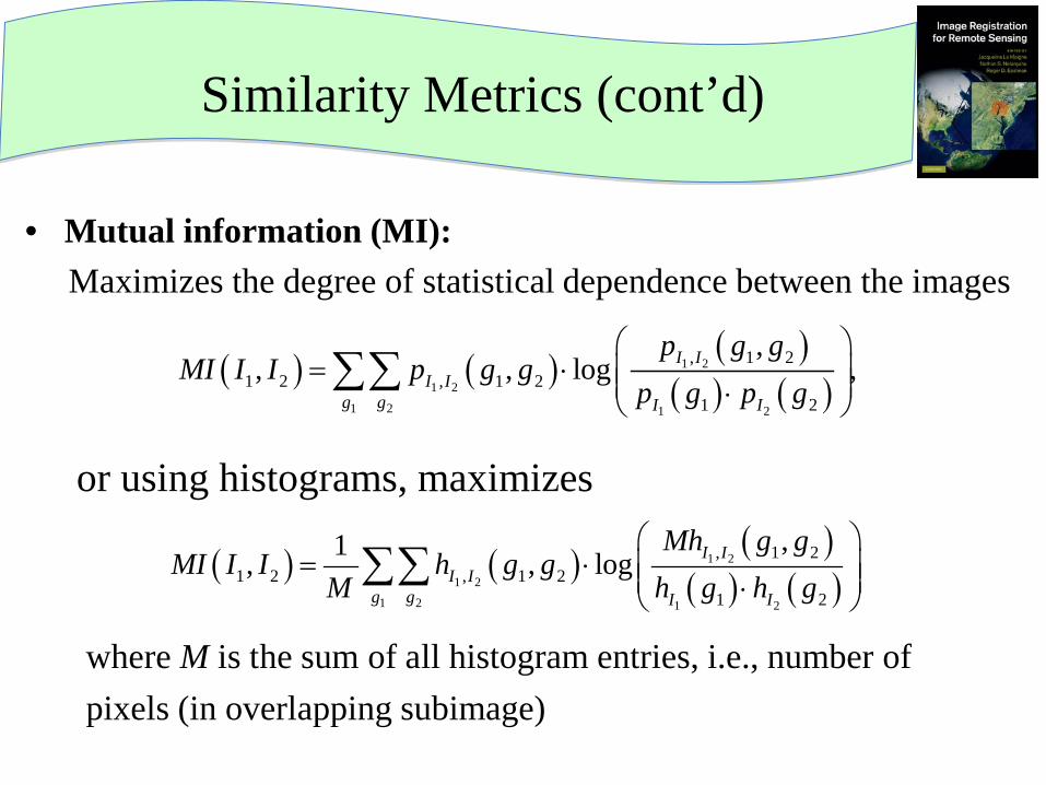
• Mutual information (MI): Maximizes the degree of statistical dependence between the images
or using histograms, maximizes where M is the sum of all histogram entries, i.e., number of pixels (in overlapping subimage)
Similarity Metrics (cont’d)
( ) ( ) ( )( ) ( )
1 2
1 2
1 2 1 2
, 1 21 2 , 1 2
1 2
,, , log ,I I
I Ig g I I
p g gMI I I p g g
p g p g
= ⋅ ⋅ ∑∑
( ) ( ) ( )( ) ( )
1 2
1 2
1 2 1 2
, 1 21 2 , 1 2
1 2
,1, , log I II I
g g I I
Mh g gMI I I h g g
M h g h g
= ⋅ ⋅ ∑∑

Similarity Metrics (cont’d)
MI vs. -norm and NCC applied to Landsat-5 images (source: H. Chen et al. ‘03)
2L

• Partial Hausdorff distance (PHD): where (Huttenlocher et al. ‘93, Mount et al. ‘99)
Similarity Metrics (cont’d)
1K =
2K =
1K I=
( ) ( )1 1 2 21 2 1 2, min dist , ,th
K p I p IH I I K p p∈ ∈=
11 K I≤ ≤

• Discrete Gaussian mismatch (DGM): where denotes the weight of point a, and
is similarity measure ranging between 0 and 1(Mount et al., Ch. 8)
Similarity Metrics (cont’d)
22
2
dist( , )( ) exp2a Iw aσ σ
= −
11 2
1
( )DGM ( , ) 1
| |a I
w aI I
Iσ
σ∈= −
∑
( )w aσ

• Translation-only, rigid • Rotation, scale, and translation (RST) • Affine (6 degrees of freedom)
• Projective/homography (e.g., for perspective effects in image
mosaicing; Govindu and Chellappa, Ch. 10); 8 parameters
Transformation Functions
cos sinsin cos0 0 1
x
p y
s s tT s s t
θ θθ θ
− =
' cos sin' sin cos
x
y
x s x s y ty s x s y t
θ θθ θ
= ⋅ − ⋅ += ⋅ + ⋅ +

• Weighted linear transformation (Goshtasby, Ch. 7); adaptive transformation, continuous and smooth, applied to multiview images with local geometric differences, and maps an entire image to another – Interpolating surface is a weighted sum of planar patches,
each of which passes through a control point and provides a desired gradient, i.e.,
Transformation Functions (cont’d)
iiiiii FyybxxayxL +−+−= )()(),(
∑∑
=
== n
i i
n
i ii
yxR
yxLyxRyxf
1
1
),(
),(),(),(
[ ] 2122 )()(),( −
−+−= iii yyxxyxRfor monotonically decreasing weight
and

Transformation Functions (cont’d)
Source: Goshtasby, IR Tutorial, CVPR ‘11
Reference Sensed
Registered

Correlation L2-norm MI Hausdorff distance
FFT
Robust feature
matching Gradient descent
Spall’s optimization
Thévenaz, Ruttimann,
Unser optimization
Gray levels Spline or Simoncelli LPF
Simoncelli BPF
L2-norm MI
Gradient descent
Spall’s optimization
Thévenaz, Ruttimann,
Unser optimization
IR Components (Revisited)
Features
Similarity measure
Matching strategy

• Exhaustive search (exponential in dimensionality of space) • Fast Fourier transform (FFT) • Numerical optimization (e.g., steepest gradient descent wrt SSD,
NCC, and MI (Thévenaz, Ruttimann, and Unser (TRU) ‘98; Spall ‘92))
• Robust transformation estimate (e.g., RANSAC, LMS) if (most) correspondences are known (via SIFT-like)
• “Correspondenceless”, e.g., correlation of descriptor distribution/feature consensus (Govindu et al. ‘99)
• Robust feature matching (RFM), e.g., efficient subdivision and pruning of transformation space; Huttenlocher et al. ‘93, Mount et al. ’99, Netanyahu et al. ‘04
Matching Strategies
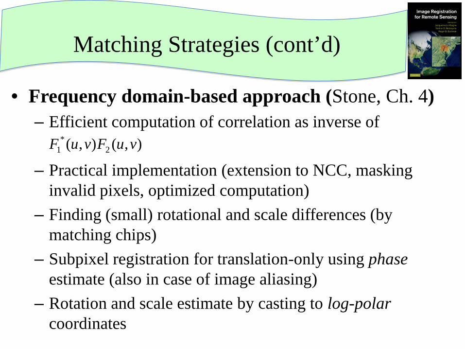
• Frequency domain-based approach (Stone, Ch. 4) – Efficient computation of correlation as inverse of – Practical implementation (extension to NCC, masking
invalid pixels, optimized computation) – Finding (small) rotational and scale differences (by
matching chips) – Subpixel registration for translation-only using phase
estimate (also in case of image aliasing) – Rotation and scale estimate by casting to log-polar
coordinates
Matching Strategies (cont’d)
),(),( 2*
1 vuFvuF

• Matched filtering (Q. Chen, Ch. 5) – Maximize SNR (using theory of linear systems) – Apply phase-only and symmetric phase-only matched filters for
translation-only IR
– Apply Fourier-Mellin transform for rotation and scale changes; transform represents these parameters as translational shifts in log-polar coordinates of magnitude of Fourier spectrum, i.e., first estimate rotation and scale, followed by translation estimate
Matching Strategies (cont’d)
)(
2
2
1
*1
),(),(
),(),(product Phase yx vtutje
vuFvuF
vuFvuF +−==

Matching Strategies (cont’d)
Pair of SPOT images and their registration, using symmetric phase-only matched filters on their Fourier-Mellin transforms
Rotation and scale estimate
Translation estimate
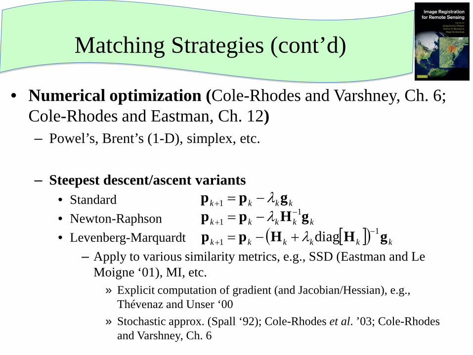
• Numerical optimization (Cole-Rhodes and Varshney, Ch. 6; Cole-Rhodes and Eastman, Ch. 12) – Powel’s, Brent’s (1-D), simplex, etc. – Steepest descent/ascent variants
• Standard • Newton-Raphson • Levenberg-Marquardt
– Apply to various similarity metrics, e.g., SSD (Eastman and Le Moigne ‘01), MI, etc.
» Explicit computation of gradient (and Jacobian/Hessian), e.g., Thévenaz and Unser ‘00
» Stochastic approx. (Spall ‘92); Cole-Rhodes et al. ’03; Cole-Rhodes and Varshney, Ch. 6
Matching Strategies (cont’d)
kkkk gpp λ−=+1
kkkkk gHpp 11
−+ −= λ
[ ]( ) kkkkkk gHHpp 11 diag −+ +−= λ

Matching Strategies (cont’d)
Pair of Landsat images over DC
MI surfaces of above (level 1 and 4) images, using B-spline interpolation (Cole-Rhodes and Varshney, Ch. 6)

• Alignment via local geometric distributions (Govindu and Chellappa, Ch. 10)
Matching Strategy (cont’d)
Rotated contours
Slope angle distributions and their correlation

• Robust feature matching (RFM) (Mount et al., Ch. 8) – Space of affine transformations: 6-D space – Subdivide: Quadtree or kd-tree. Each cell T represents a set
of transformations; T is active if it may contain ; o/w, it is killed
– Uncertainty regions (UR’s): Rectangular approximation to the possible images for all
– Bounds: Compute upper bound (on optimum similarity) by sampling a transformation and lower bound by computing nearest neighbors to each UR
– Prune: If lower bound exceeds best upper bound, then kill the cell; o/w, split it
Matching Strategy (cont’d)
( )aτ 1,T a Iτ ∈ ∈
optt
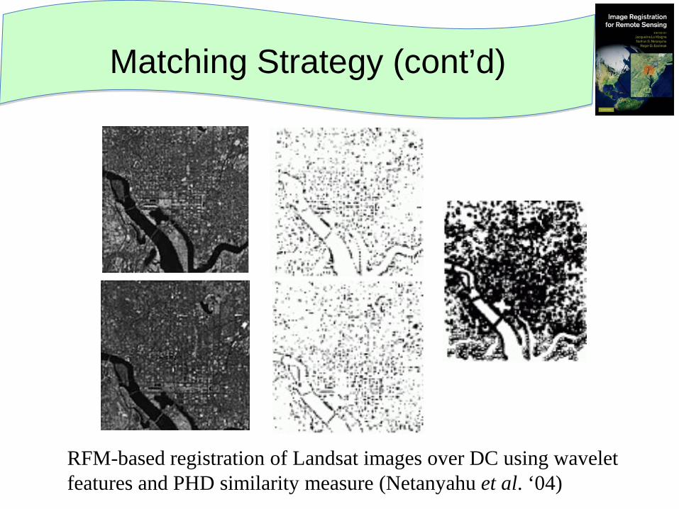
Matching Strategy (cont’d)
RFM-based registration of Landsat images over DC using wavelet features and PHD similarity measure (Netanyahu et al. ‘04)

• Computational efficiency – “Culling” feature points via, e.g., condition theory
(Kenney et al. ‘03, Ch. 9) – Efficient numerical or discrete algorithmic
procedures – Hierarchical pyramid-like (wavelet) decomposition – Use landmark chip database (instead of a large
scene) or alternatively, extract automatically corresponding regions of interest using mathematical morphology (Plaza et al. ‘05, ‘07)
Matching Strategy (cont’d)

• Use Cramér-Rao bounds as performance benchmark for performance evaluation of image registration (Xu and Varshney, Ch. 13)
Miscellaneous

From Theory to Practice Operational Requirements
Roger D. Eastman Loyola University, Baltimore,
Maryland

Why isn’t this problem solved by now?
• A wealth of approaches! • SIFT, ASIFT, BSIFT, SIFT/NCC, SIFT/FLOUR
• Beat the problem to death with terminology • “Assume we have a Banach space …”
• Many smart people wielding heavy mathematical weapons
against a relatively fixed problem– why hasn’t the problem yielded? Why no gold standard algorithm?

But it is solved … ask LANDSAT
Operational Satellite Teams solve it every day •GOES –Carr, Chapter 15 •MISR – Jovanovic et al, Chapter 16 •AVHRR – Emery et al, Chapter 17 •Landsat, Storey, Chapter 18 •SPOT, Ballarin, Chapter 19 •VEGETATION, Sylvander, Chapter 20 •MODIS, Wolfe et al, Chapter 21 •SeaWiFS, Patt, Chapter 22

And it’s often solved the old-fashioned way (2008) – Normalized Cross Co

Example: Landsat ETM+
• Geodetic accuracy – Database of GCPs derived from USGS data – Normalized correlation – Updates navigation models – Results: RMSE ~54m
• Band-to-band registration – Selected tie-points in high-freq. arid regions – Normalized correlation – Subpixel by second order fit to 3x3 neighborhood – Result: 0.1 to 0.2 subpixel

Operational teams requirements
• Know models of sensor/platform/ • Have access to complete data set • Have continuing demands/responsibility • Are registering same plots of land again and
again – can invest effort in data preparation • Can’t take big risks on unproven methods

Know platform: Landsat team knowledge
• Sensor geometry – Band to band
• Sensor to platform – Sensor to sensor
• Orbit – Platform to Earth
• Terrain data – DEM
• Radiometric model
Illustrations USGS/NASA

Invest in data: ETM+ Chips

Know data: GOES channel 1 (Baja)
• Contrast reversal day to night
• Requires use of contour matching

Use DEMs: Digital Terrain Models
Taking terrain into account in matching

Use proven methods: Landsat 7 library
• Clean data, go fast – Use Normalized Grey-Scale Correlation
• Missing data/gaps, need robustness – Use Mutual Information
• Available alternative – Use Robust Feature Matching

End Users – Earth scientists
• Know what data is for • Have to fuse many data sets • Have access to ancillary data • Know cultural and historical data
• Don’t need one magic method – need toolbox
of many approaches

Missouri river 1804-2002
Illustrations U Missouri Geography Department

Institutional challenges to “solving” IR for RS
• Different communities/literature/requirements – Photogrammetry – Computer vision/image processing – Operational teams – Remote sensing/Earth scientists/end users
• Demanding/varying mission requirements – Caution in system design, new methods
• Expensive sensors and images – Hard to share data or complete models

Conclusion
Jacqueline Le Moigne Nathan S. Netanyahu
Roger D. Eastman

THE FUTURE OF IMAGE REGISTRATION
• Satellite sensing/imaging in full expansion – Explosion of commercial satellites – Exploring distant planets (Moon, Mars, etc.), e.g. Lunar Reconnaissance Orbiter
(LRO) • Future research and challenges
– Combining multiple band-to-band registrations (e.g., hyperspectral data) – Automatically extracting windows of interest (decreasing processing time and
increasing accuracy) – Dealing with other data sources (e.g., planetary imagery, or verification of
optical systems) – Integration and fusion of multiple source imagery (various satellites, vector map,
airborne, ground data, etc.) – Onboard implementations on specialized hardware – Multistage registration algorithms combining multiple principles and approaches
and utilizing interdisciplinary systems engineering approach , thus increasing algorithms robustness and applicability

Other Memories, 1983 to 1988 …

The Autonomous Land Vehicle (ALV) Project in Colo
Thank You!
Jacqueline Le Moigne Nathan S. Netanyahu
Roger D. Eastman


![[REMOTE SENSING] 3-PM Remote Sensing](https://img.dokumen.tips/doc/110x75/61f2bbb282fa78206228d9e2/remote-sensing-3-pm-remote-sensing.jpg)

