Embed Size (px)
Citation preview
Image Processing and Representations
Prepared by Behzad Sajadi
Borrowed from Frédo Durand’s Lectures at MIT

Image processing
• Filtering, Convolution, and our friend Joseph Fourier
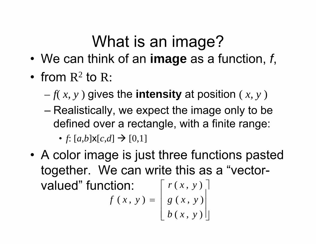
What is an image?• We can think of an image as a function, f,• from R2 to R:
– f( x, y ) gives the intensity at position ( x, y ) – Realistically, we expect the image only to be
defined over a rectangle, with a finite range:• f: [a,b]x[c,d] [0,1]
• A color image is just three functions pasted together. We can write this as a “vector-valued” function: ( , )
( , ) ( , )( , )
r x yf x y g x y
b x y
⎡ ⎤⎢ ⎥= ⎢ ⎥⎢ ⎥⎣ ⎦

Images as functions
x
yf(x,y)

Image Processing
• image filtering: change range of image• g(x) = h(f(x))f
xh
f
x
f
x
hf
x
• image warping: change domain of image• g(x) = f(h(x))

Image Processing
• image filtering: change range of image• g(x) = h(f(x))
h
h
• image warping: change domain of image• g(x) = f(h(x))

Point Processing
• The simplest kind of range transformations are those independent of position x,y:
• g = t(f)• This is called point processing.
• Important: every pixel for himself – spatial information completely lost!
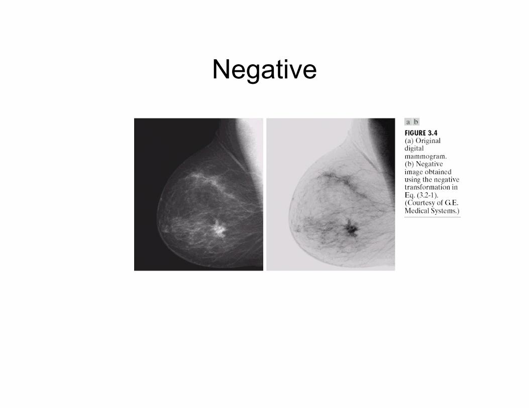
Negative
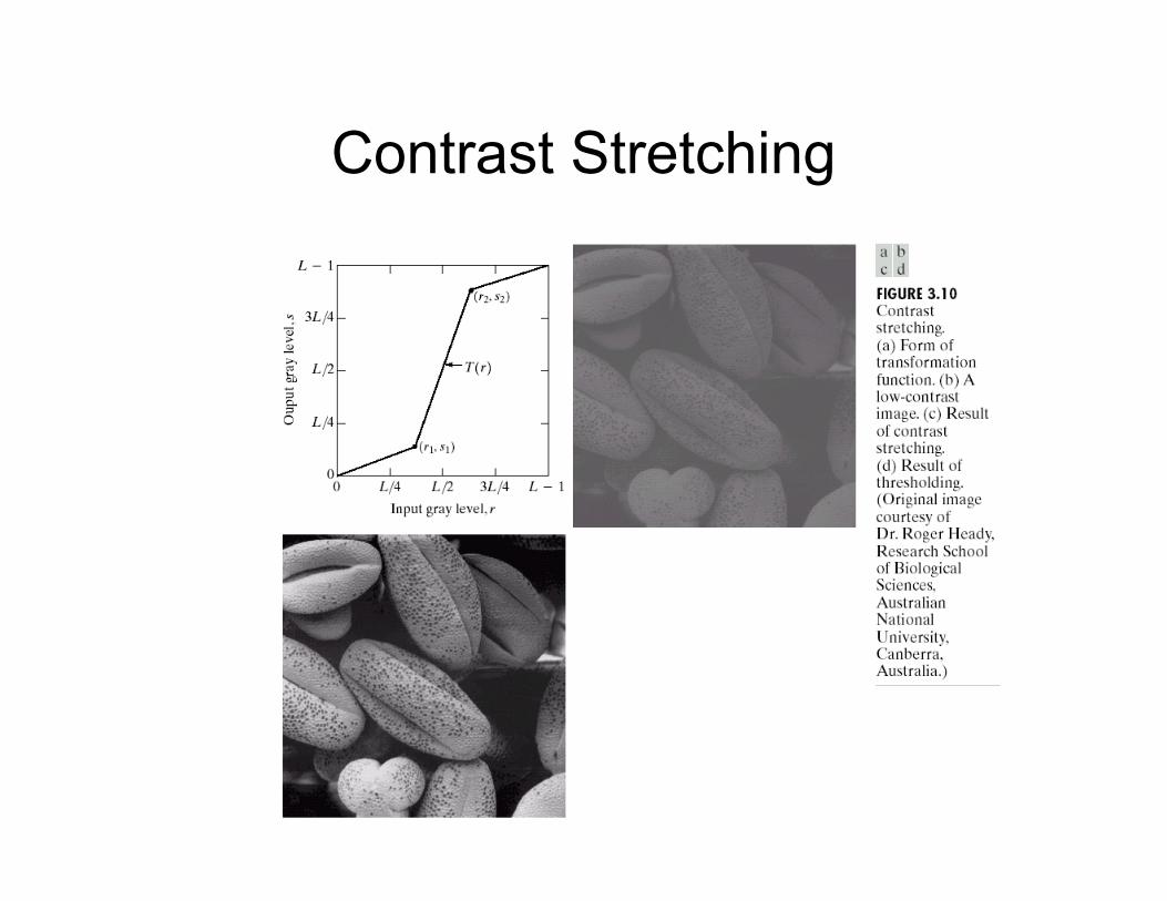
Contrast Stretching

Image Histograms
Cumulative Histograms
s = T(r)
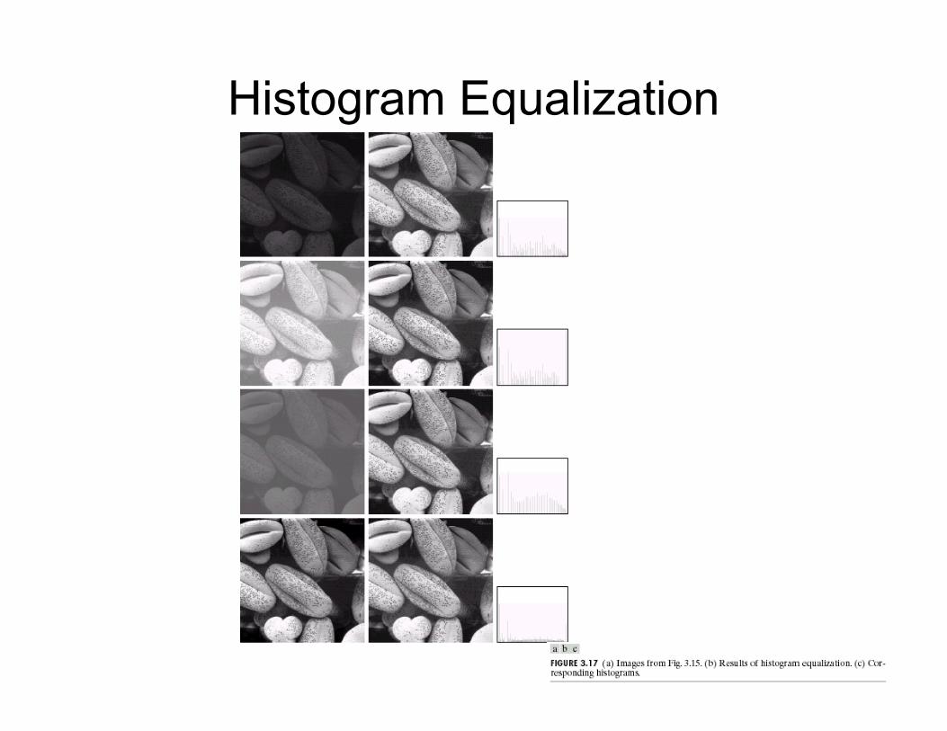
Histogram Equalization

Questions?

Filtering
• So far we have looked at range-only and domain-only transformation
• But other transforms need to change the range according to the spatial neighborhood– Linear filtering in particular
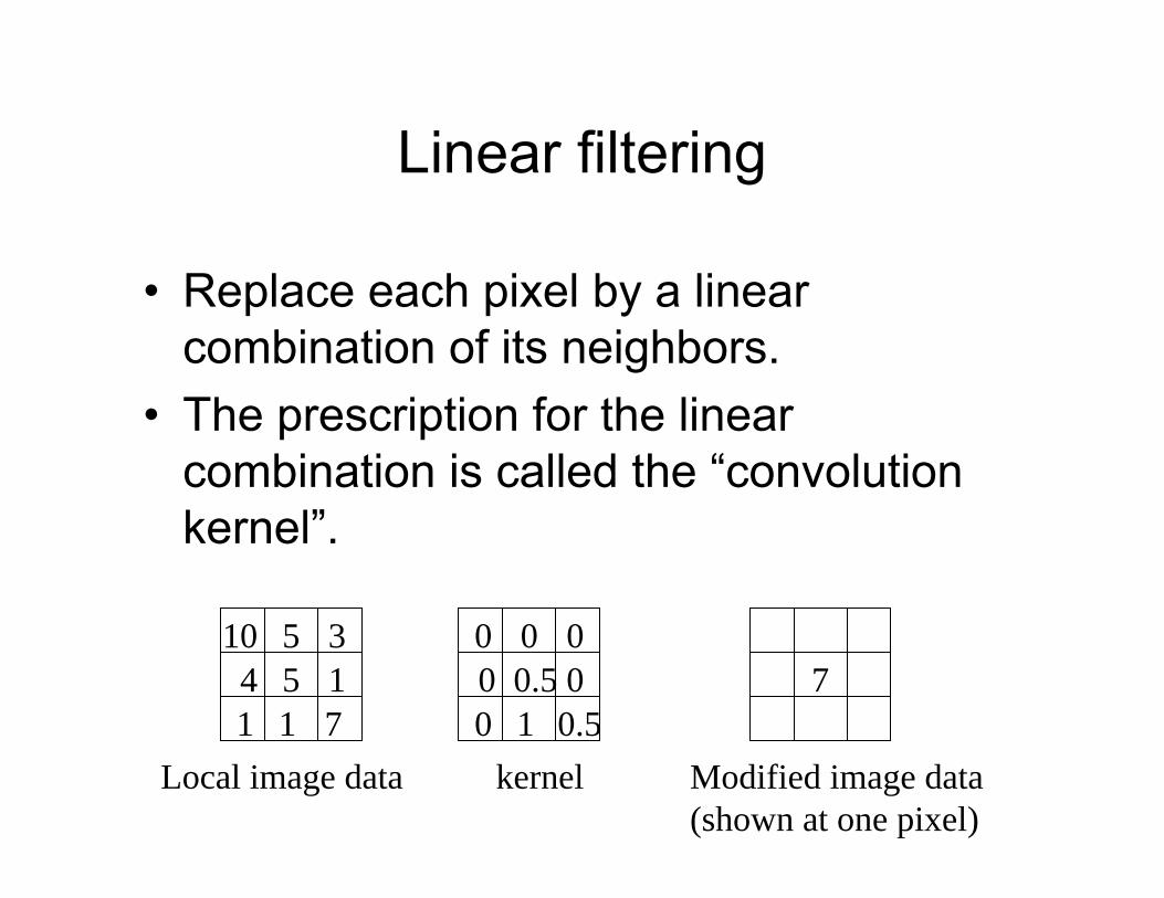
Linear filtering
• Replace each pixel by a linear combination of its neighbors.
• The prescription for the linear combination is called the “convolution kernel”.
5 141 71
5 310
0.50.5 0010
0 00
Local image data kernel
7
Modified image data(shown at one pixel)

More formally: Convolution
∑ −−=⊗=lk
lkglnkmIgInmf,
],[],[],[
I
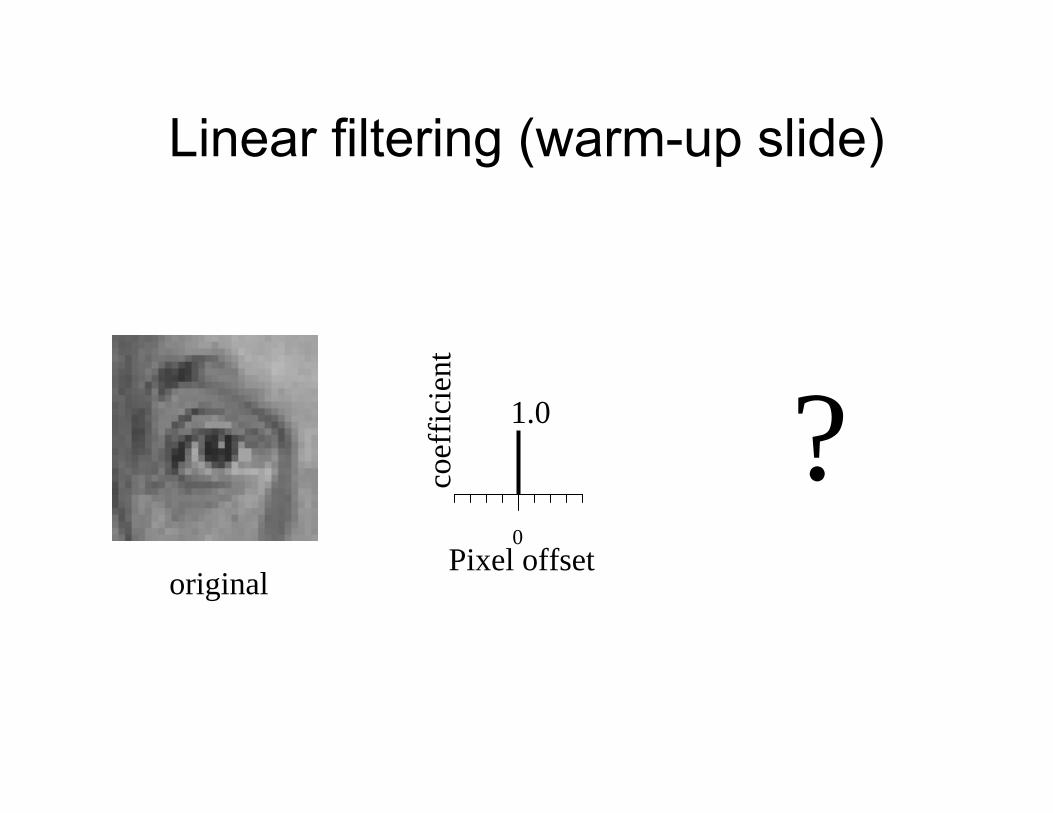
Linear filtering (warm-up slide)
original0
Pixel offset
coef
ficie
nt1.0 ?

Linear filtering (warm-up slide)
original0
Pixel offset
coef
ficie
nt1.0
Filtered(no change)

Linear filtering
0Pixel offset
coef
ficie
nt
original
1.0
?

shift
0Pixel offset
coef
ficie
nt
original
1.0
shifted
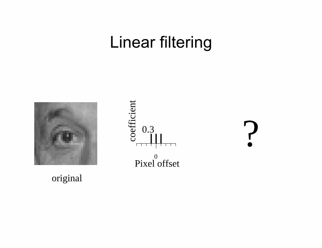
Linear filtering
0Pixel offset
coef
ficie
nt
original
0.3 ?
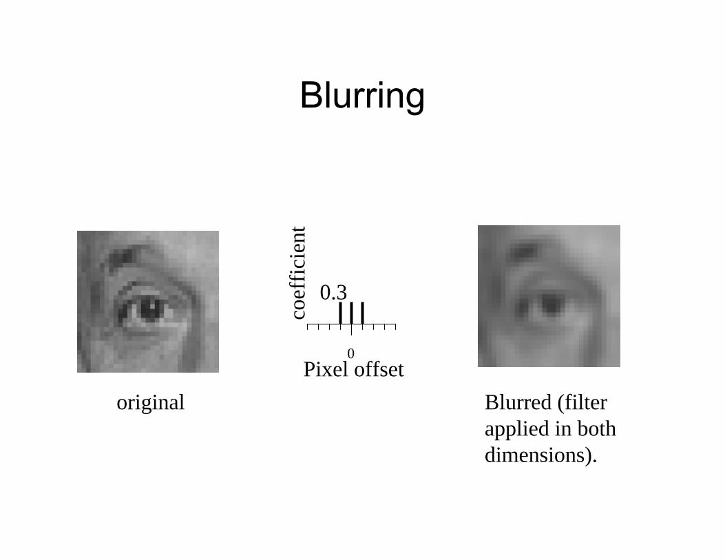
Blurring
0Pixel offset
coef
ficie
nt
original
0.3
Blurred (filterapplied in both dimensions).

Blur examples
0Pixel offset
coef
ficie
nt
0.3
original
8
filtered
2.4
impulse
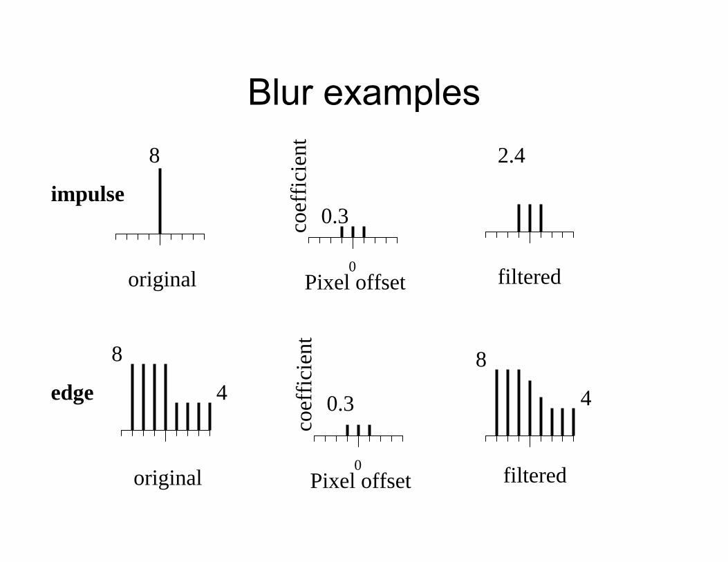
Blur examples
0Pixel offset
coef
ficie
nt
0.3
original
8
filtered
48
4
impulse
edge
0Pixel offset
coef
ficie
nt
0.3
original
8
filtered
2.4

Questions?
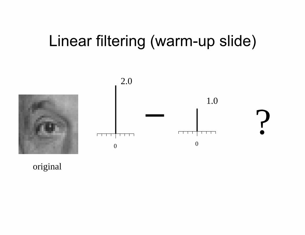
Linear filtering (warm-up slide)
original
0
2.0
?0
1.0
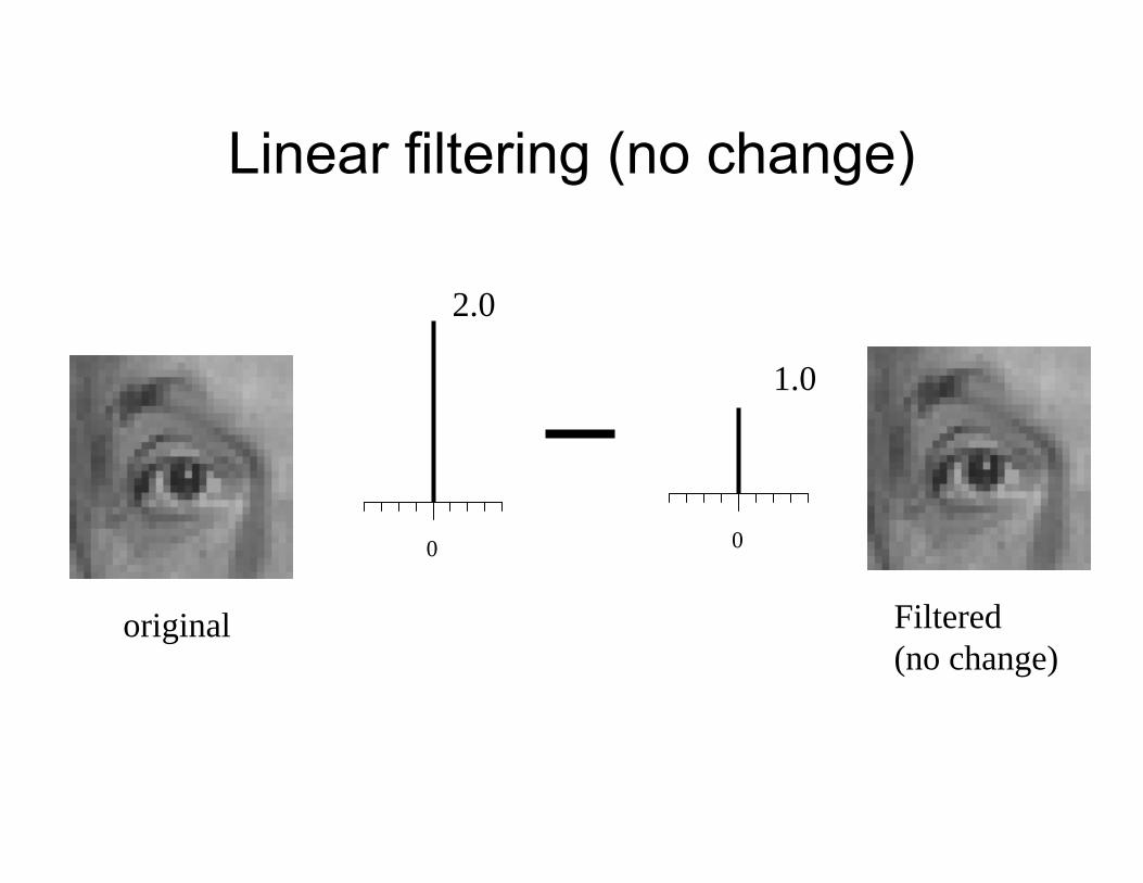
Linear filtering (no change)
original
0
2.0
0
1.0
Filtered(no change)
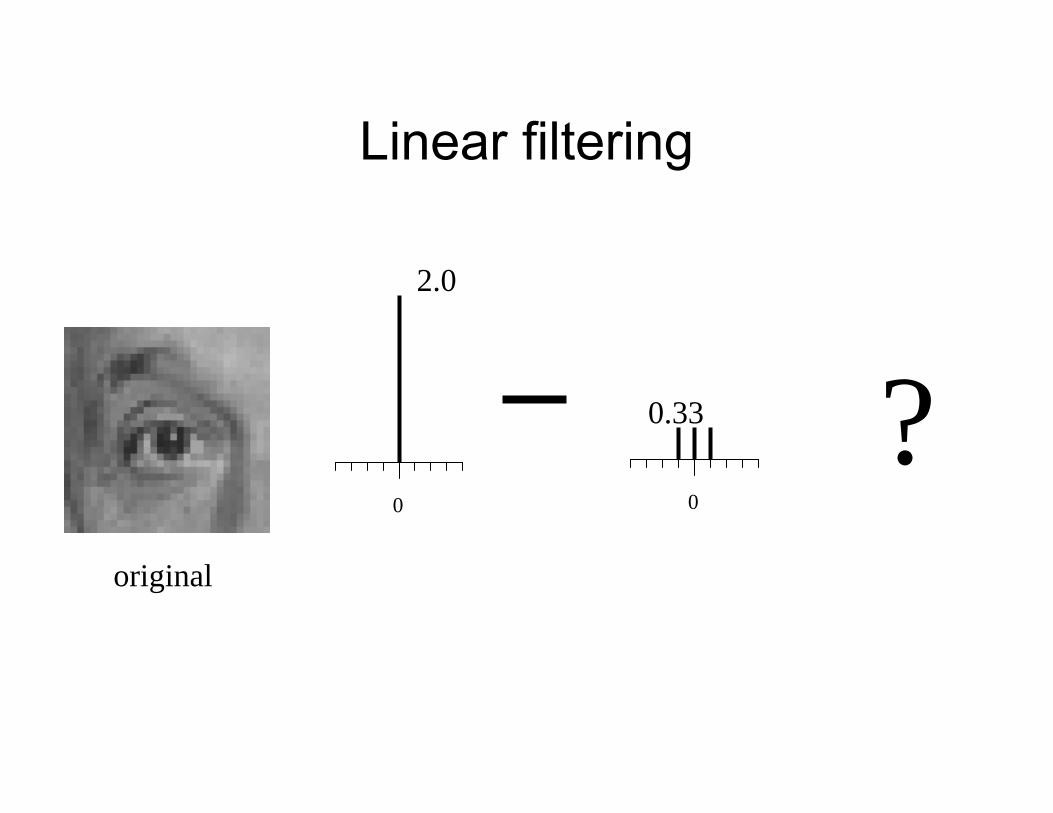
Linear filtering
original
0
2.0
0
0.33 ?
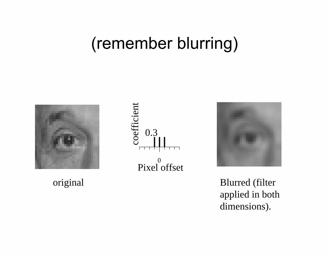
(remember blurring)
0Pixel offset
coef
ficie
nt
original
0.3
Blurred (filterapplied in both dimensions).

Sharpening
original
0
2.0
0
0.33
Sharpened original

Sharpening example
coef
ficie
nt
-0.3original
8
Sharpened(differences are
accentuated; constantareas are left untouched).
11.21.7
-0.25
8
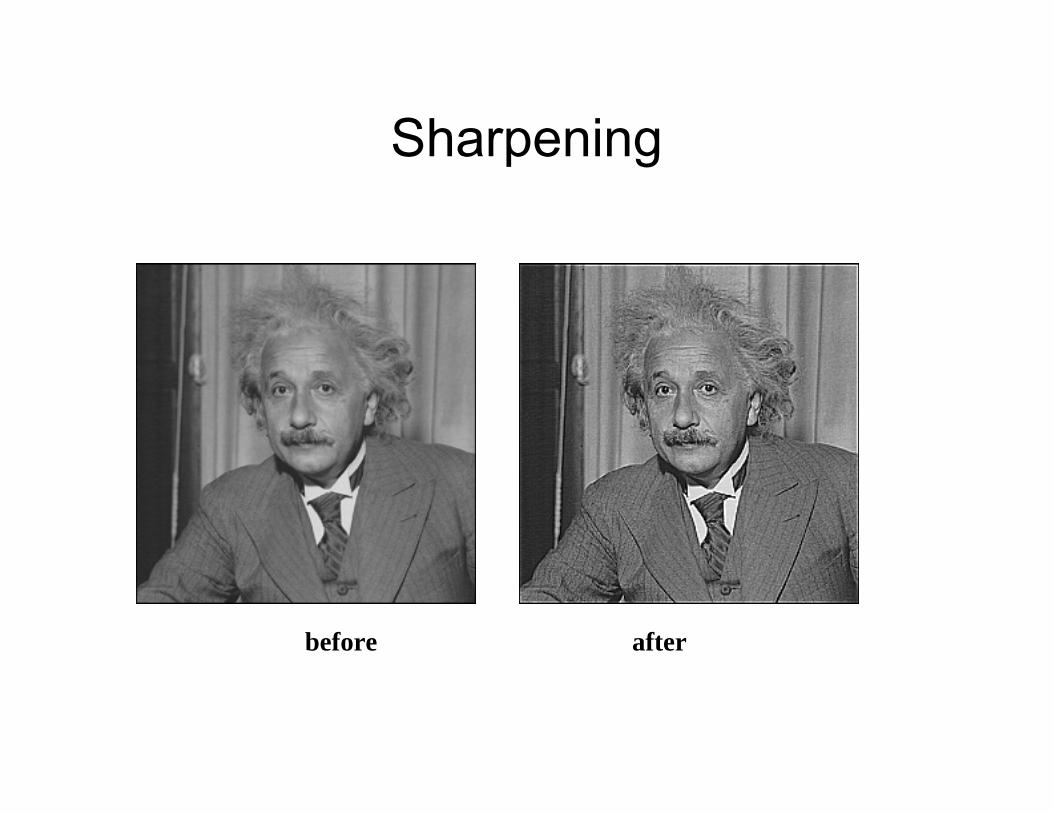
Sharpening
before after

Questions?
Studying convolutions
• Convolution is complicated– But at least it’s linear
(f+kg)- h = f-h +kg• We want to find a better expression
– Let’s study function whose behavior is simple under convolution

Blurring: convolution
Input KernelConvolution
sign
Same shape, just reduced contrast!!!
This is an eigenvector (output is the input multiplied by a constant)

Big Motivation for Fourier analysis
• Sine waves are eigenvectors of the convolution operator

Other motivation for Fourier analysis: sampling
• The sampling grid is a periodic structure– Fourier is pretty good at handling that– A sine wave can have serious problems with sampling
• Sampling is a linear process
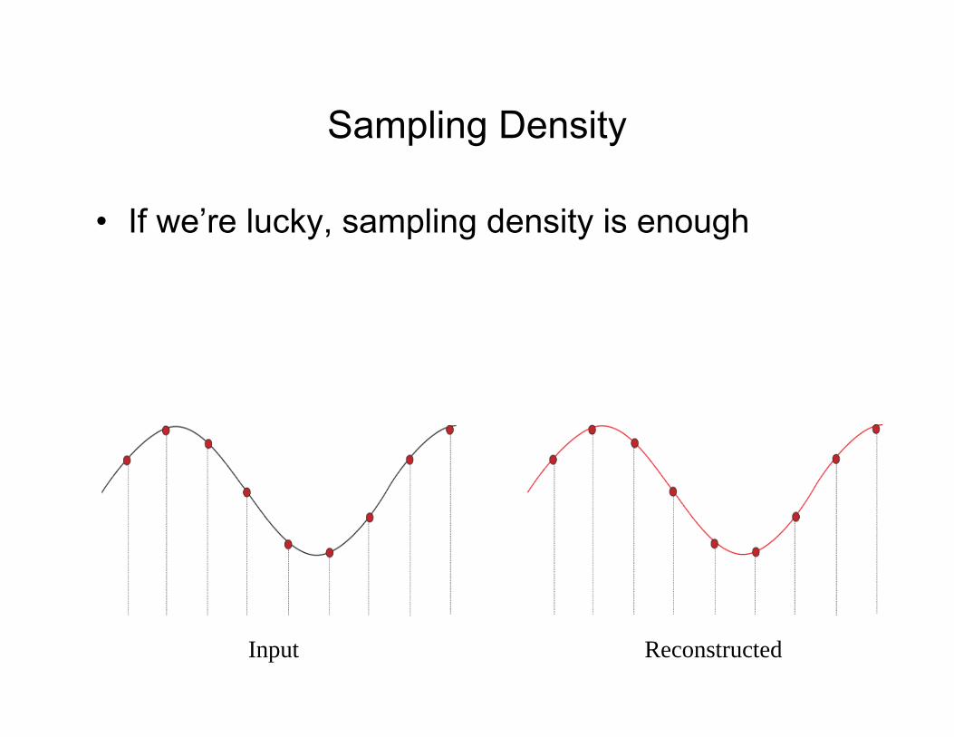
Sampling Density
• If we’re lucky, sampling density is enough
Input Reconstructed

Sampling Density
• If we insufficiently sample the signal, it may be mistaken for something simpler during reconstruction (that's aliasing!)
Motivation for sine waves
• Blurring sine waves is simple– You get the same sine wave, just scaled down– The sine functions are the eigenvectors of the
convolution operator• Sampling sine waves is interesting
– Get another sine wave– Not necessarily the same one! (aliasing)
If we represent functions (or images) with a sum of sine waves, convolution and sampling are easy to study

Questions?
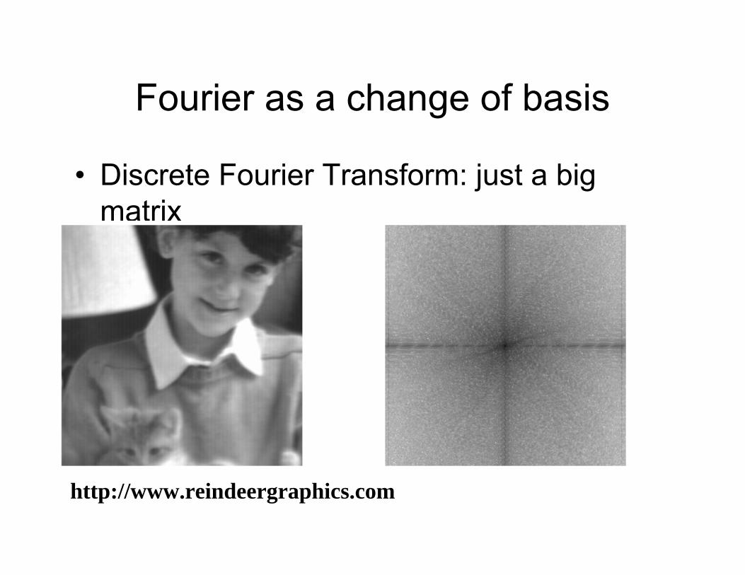
Fourier as a change of basis
• Discrete Fourier Transform: just a big matrix
• But a smart matrix!
http://www.reindeergraphics.com
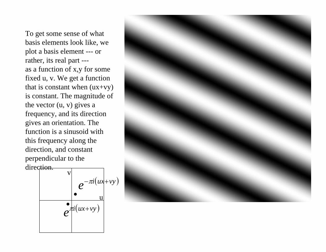
To get some sense of what basis elements look like, we plot a basis element --- or rather, its real part ---as a function of x,y for some fixed u, v. We get a function that is constant when (ux+vy) is constant. The magnitude of the vector (u, v) gives a frequency, and its direction gives an orientation. The function is a sinusoid with this frequency along the direction, and constant perpendicular to the direction.
u
v( )vyuxie +−π
( )vyuxie +π

Here u and v are larger than in the previous slide.
u
v( )vyuxie +−π
( )vyuxie +π
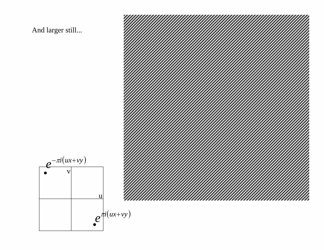
And larger still...
u
v( )vyuxie +−π
( )vyuxie +π

Motivations
• Computation bases– E.g. fast filtering
• Sampling rate and filtering bandwidth• Optics: wave nature of light & diffraction • Insights

Questions?
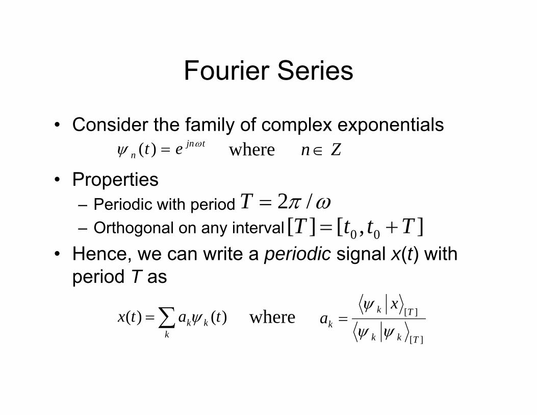
Fourier Series
• Consider the family of complex exponentials
• Properties– Periodic with period– Orthogonal on any interval
• Hence, we can write a periodic signal x(t) with period T as
tjnn et ωψ =)( Zn ∈
ωπ /2=T],[][ 00 TttT +=
∑=k
kk tatx )()( ψ][
][
Tkk
Tkk
xa
ψψ
ψ=
where
where
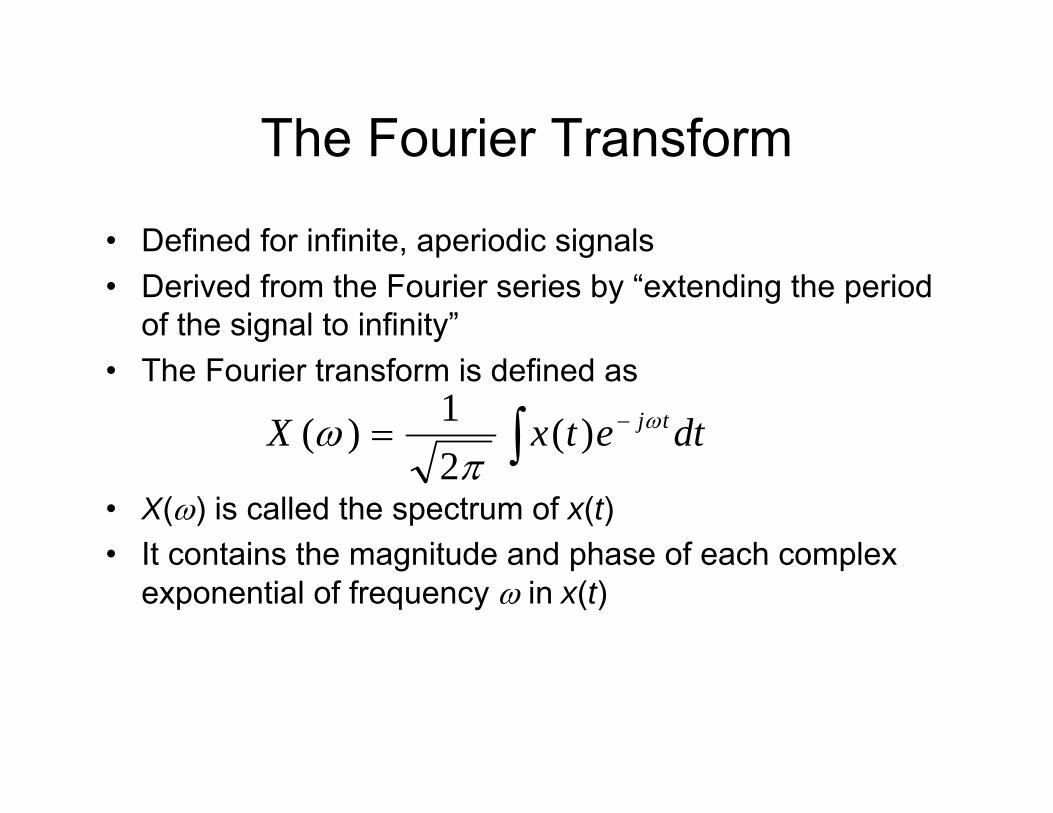
The Fourier Transform
• Defined for infinite, aperiodic signals• Derived from the Fourier series by “extending the period
of the signal to infinity”• The Fourier transform is defined as
• X(ω) is called the spectrum of x(t)• It contains the magnitude and phase of each complex
exponential of frequency ω in x(t)
∫ −= dtetxX tjω
πω )(
21)(

The Fourier Transform
• The inverse Fourier transform is defined as
• Fourier transform pair
• x(t) is called the spatial domain representation• X(ω) is called the frequency domain
representation
∫= ωωπ
ω deXtx tj)(21)(
)()( ωXtx F⎯→←
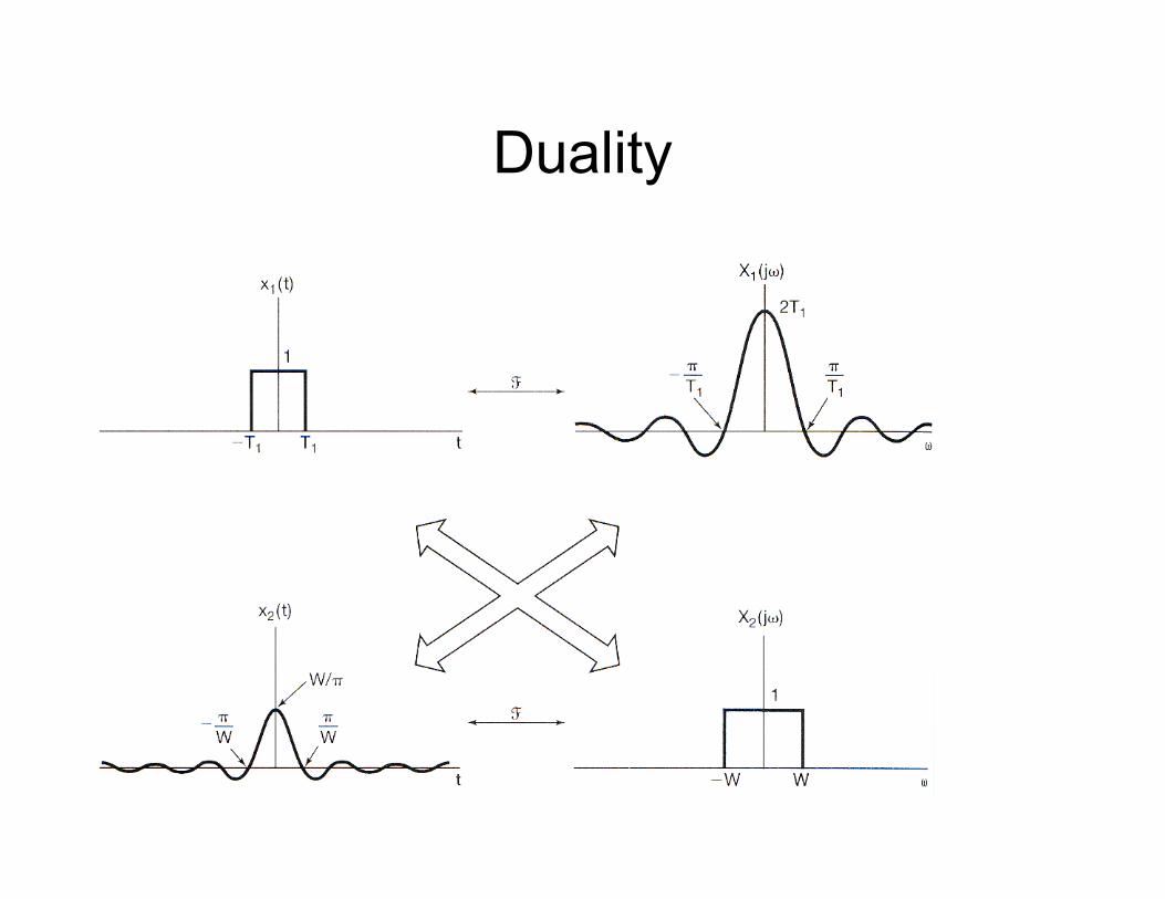
Duality
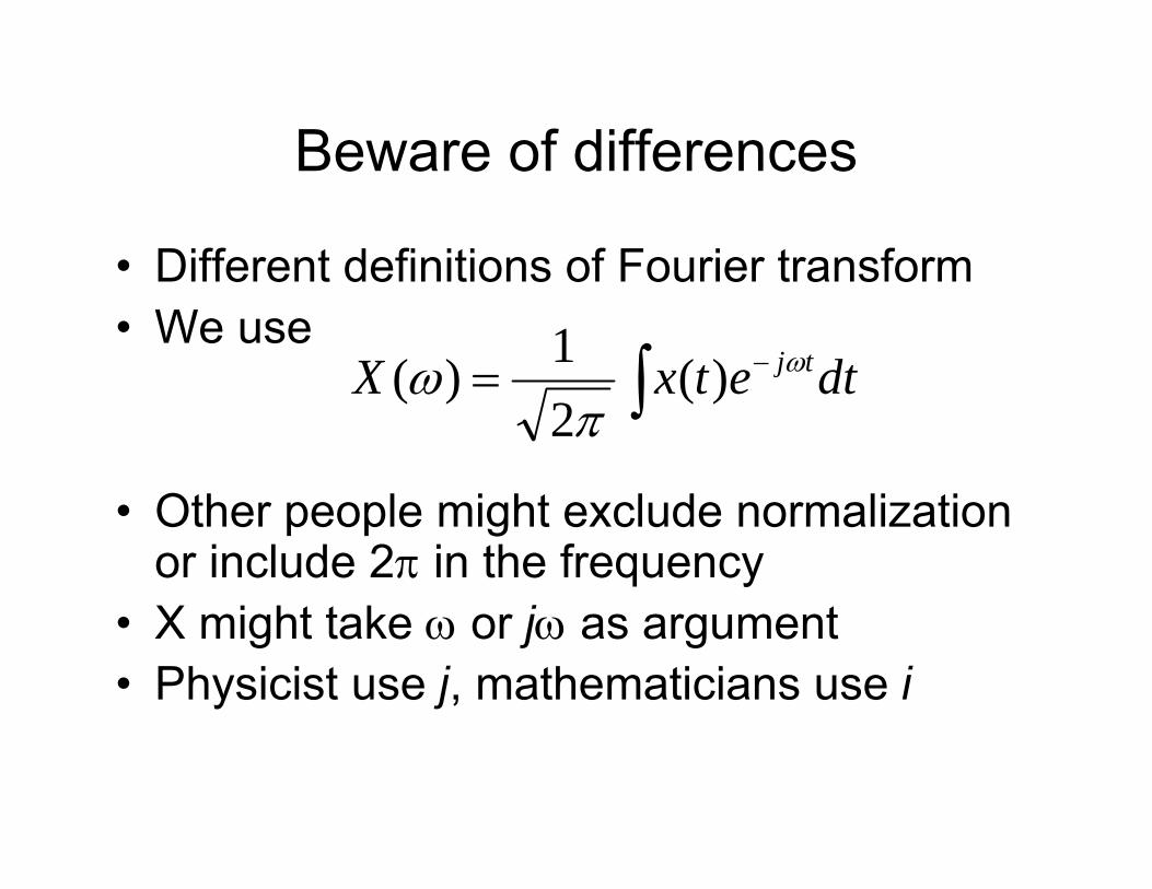
Beware of differences
• Different definitions of Fourier transform• We use
• Other people might exclude normalization or include 2π in the frequency
• X might take ω or jω as argument• Physicist use j, mathematicians use i
∫ −= dtetxX tjω
πω )(
21)(

Questions?

Phase• Don’t forget the phase! Fourier transform results
in complex numbers
• Can be seen as sum of sines and cosines
• Or modulus/phase
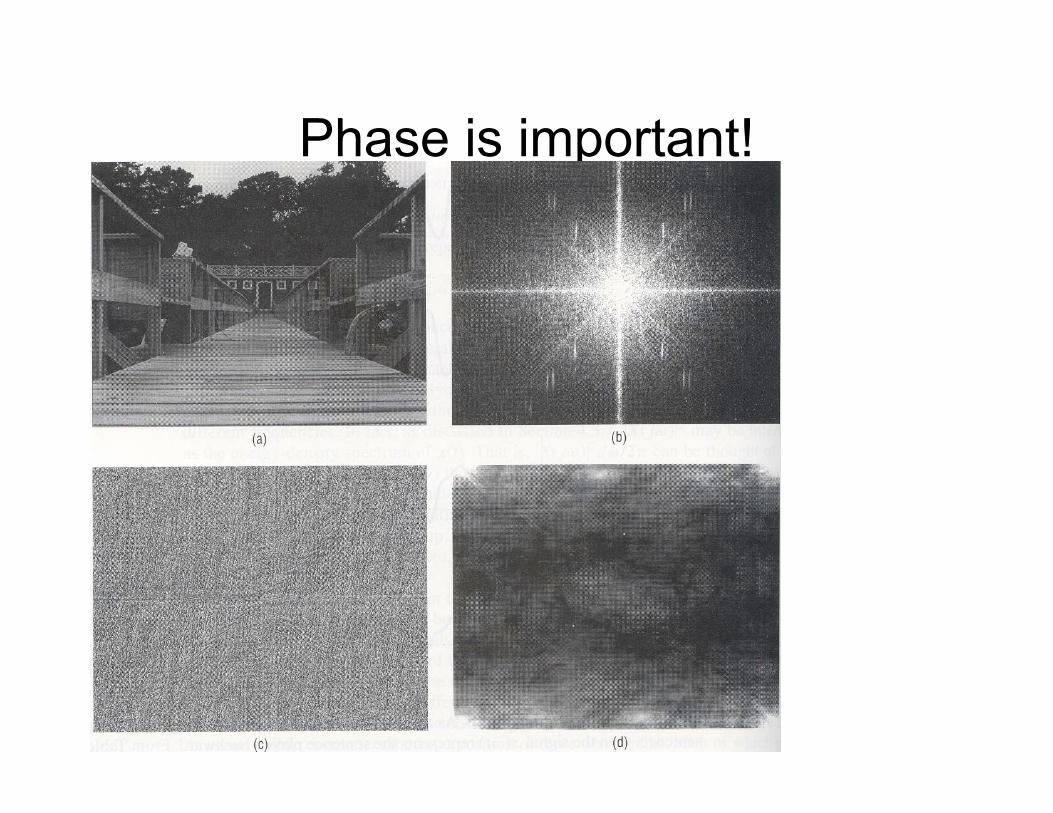
Phase is important!
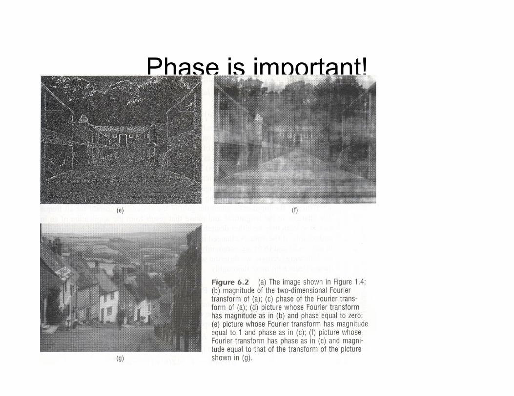
Phase is important!

Questions?

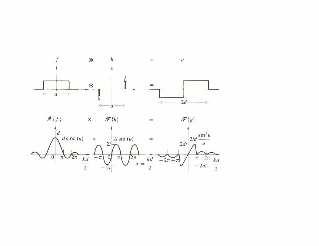
Convolution
• Sliding window

Convolution

Low pass http://www.reindeergraphics.com
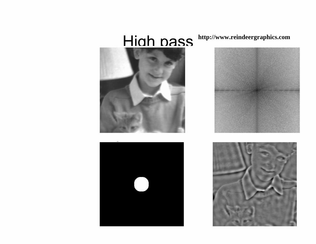
High pass http://www.reindeergraphics.com
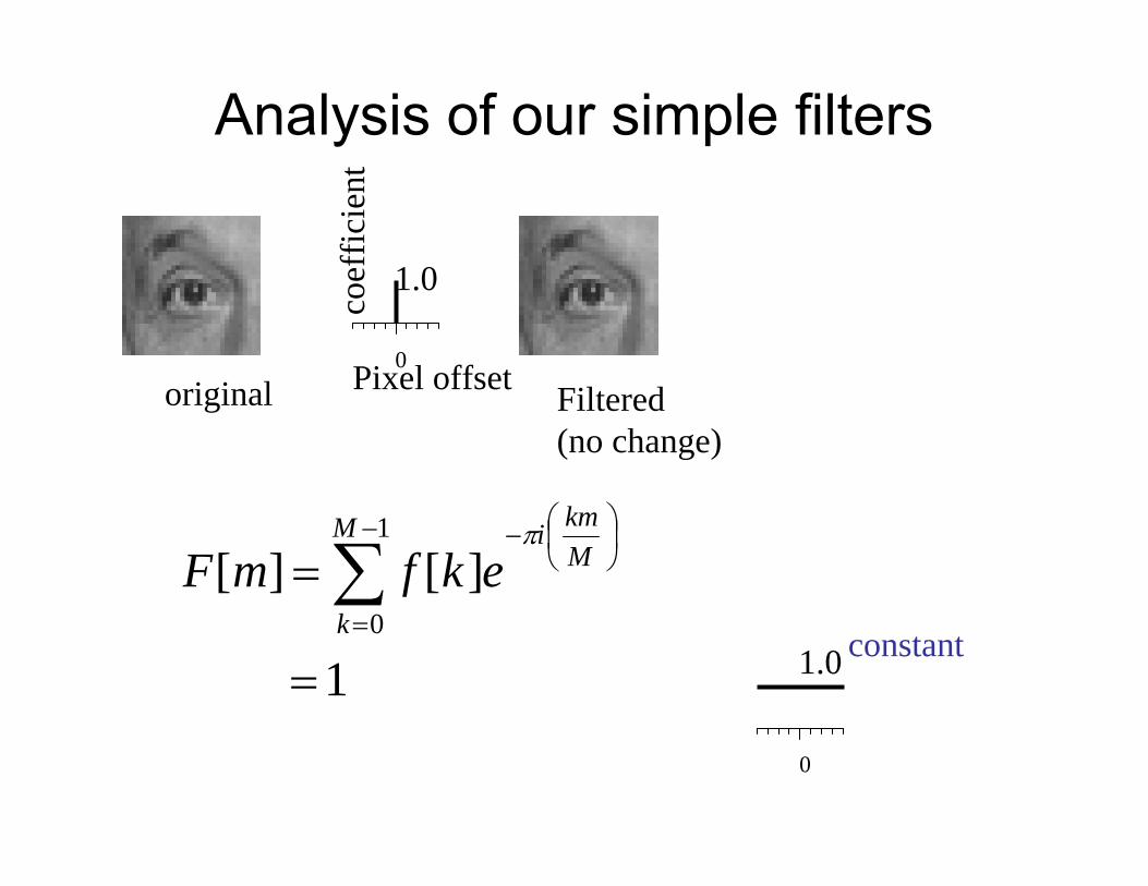
Analysis of our simple filters
original0Pixel offset
coef
ficie
nt
1.0
Filtered(no change)
1
][][1
0
=
= ∑−
=
⎟⎠⎞
⎜⎝⎛−M
k
Mkmi
ekfmFπ
0
1.0 constant

Analysis of our simple filters
0Pixel offset
coef
ficie
nt
original
1.0
shifted
Mmi
M
k
Mkmi
e
ekfmF
δπ
π
−
−
=
⎟⎠⎞
⎜⎝⎛−
=
= ∑
][][1
0
0
1.0
Constant magnitude, linearly shifted phase
δ

Analysis of our simple filters
0Pixel offsetco
effic
ient
original
0.3
blurred
⎟⎟⎠
⎞⎜⎜⎝
⎛⎟⎠⎞
⎜⎝⎛+=
= ∑−
=
⎟⎠⎞
⎜⎝⎛−
Mm
ekfmFM
k
Mkmi
π
π
cos2131
][][1
0 Low-pass filter
0
1.0
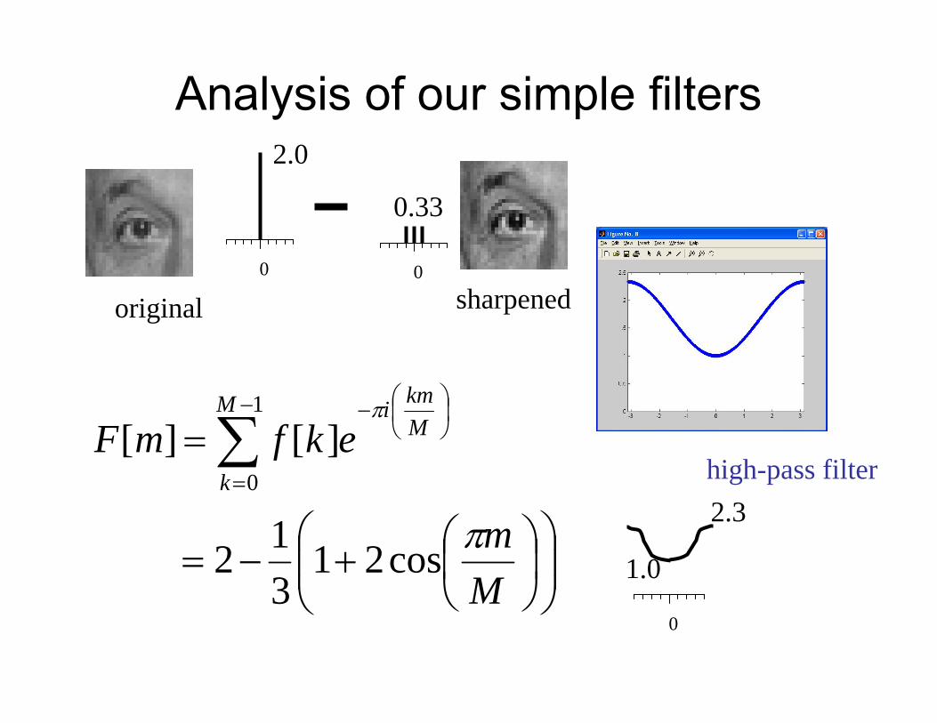
Analysis of our simple filters
original0
2.0
0
0.33
sharpened
⎟⎟⎠
⎞⎜⎜⎝
⎛⎟⎠⎞
⎜⎝⎛+−=
= ∑−
=
⎟⎠⎞
⎜⎝⎛−
Mm
ekfmFM
k
Mkmi
π
π
cos21312
][][1
0 high-pass filter
0
1.0
2.3

Questions?
Sampling and aliasing

More on Samples• In signal processing, the process of mapping a
continuous function to a discrete one is called sampling• The process of mapping a continuous variable to a
discrete one is called quantization• To represent or render an image using a computer,
we must both sample and quantize – Now we focus on the effects of sampling and how to fight them
discrete position
discretevalue
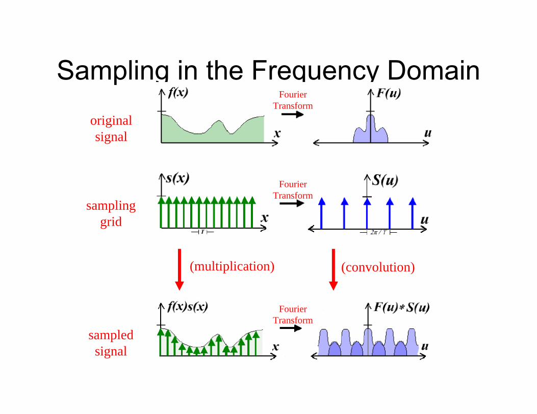
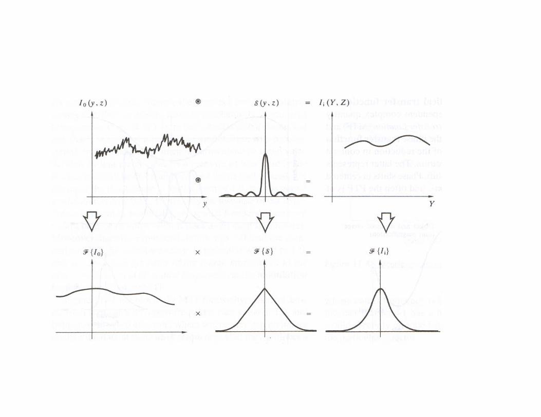
Sampling in the Frequency Domain
(convolution)(multiplication)
originalsignal
samplinggrid
sampledsignal
Fourier Transform
Fourier Transform
Fourier Transform
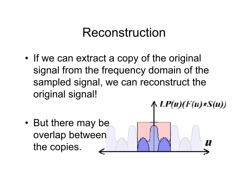
Reconstruction
• If we can extract a copy of the original signal from the frequency domain of the sampled signal, we can reconstruct the original signal!
• But there may be overlap between the copies.
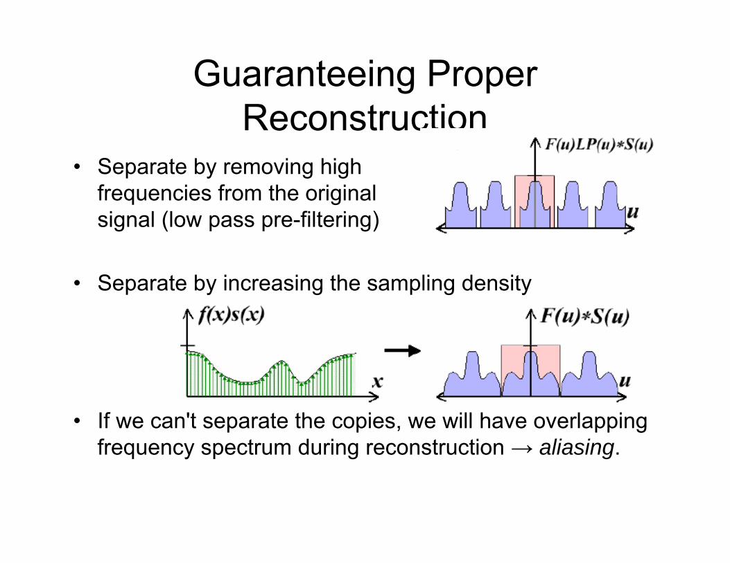
Guaranteeing Proper Reconstruction
• Separate by removing high frequencies from the original signal (low pass pre-filtering)
• Separate by increasing the sampling density
• If we can't separate the copies, we will have overlapping frequency spectrum during reconstruction → aliasing.

Sampling Theorem
• When sampling a signal at discrete intervals, the sampling frequency must be greater than twice the highest frequency of the input signal in order to be able to reconstruct the original perfectly from the sampled version (Shannon, Nyquist, Whittaker, Kotelnikov)