Embed Size (px)
Citation preview

Image Motion
COMPSCI 527 — Computer Vision
COMPSCI 527 — Computer Vision Image Motion 1 / 25

Outline
1 Image Motion
2 Constancy of Appearance
3 Motion Field and Optical Flow
4 The Aperture Problem
5 Estimating the Motion Field
6 The Lucas-Kanade Tracker
COMPSCI 527 — Computer Vision Image Motion 2 / 25

Image Motion
Continuous and Discrete Image
COMPSCI 527 — Computer Vision Image Motion 3 / 25

Image Motion
Motion Field and Displacement
x1
2x
x(t)
x(s)
• Follow the image projection x(t) of a single world point• Displacement: d(t , s) = x(t)− x(s), a difference in positions• Motion field: v(t) = dx(t)
dt , an instantaneous velocity• A field b/c it can be defined for every x in the image plane
COMPSCI 527 — Computer Vision Image Motion 4 / 25
Constancy of Appearance
Constancy of Appearance
• Images do not move• What is assumed to remain constant across images?• Motion estimation is impossible without such an assumption• Most generic assumption: The appearance of a point does
not change with time or viewpoint• If two image points in two images correspond, they look the
same• “Appearance:” Image irradiance e(x, t) (brightness)• If colors differ, so do brightnesses most of the time, so color
does not help much• We only consider gray images and video from now on
COMPSCI 527 — Computer Vision Image Motion 5 / 25

Constancy of Appearance
Constancy of Appearancex1
2x
x' = x(t)
x = x(s)
• If two image points in two images correspond, they look thesame• If x at time s and x′ at time t correspond, then
e(x, s) = e(x′, t) (finite-displacement formulation)• Equivalently, de(x(t),t)
dt = 0 (differential formulation)• This is the key constraint for motion estimation
COMPSCI 527 — Computer Vision Image Motion 6 / 25

Motion Field and Optical Flow
The Brightness Change Constraint Equation• The appearance of a point does not change with time or
viewpoint: de(x(t),t)dt = 0
• Total derivative, not partial:de(x(t), t)
dtdef= lim∆t→0
e(x(t+∆t), t+∆t)−e(x(t), t)∆t
• Use chain rule on de(x(t),t)dt = 0 to obtain the
Brightness Change Constraint Equation (BCCE)
∂e∂xT
dxdt
+∂e∂t
= 0
• v def= dx
dt is the unknown motion field• This is the key constraint for motion estimation
(Compare: ∂e(x(t),t)∂t
def= lim∆t→0
e(x(t), t+∆t)−e(x(t), t)∆t )
COMPSCI 527 — Computer Vision Image Motion 7 / 25

Motion Field and Optical Flow
Motion Field and Optical Flow• Extreme violations of constancy of appearance:
B. K. P. Horn, Robot Vision, MIT Press, 1986
• Ill-defined distinction:• Motion field ≈ true motion• Optical flow ≈ locally observed motion
• Still assume constancy of appearance almost everywhere• What else can we do?
COMPSCI 527 — Computer Vision Image Motion 8 / 25

The Aperture Problem
The Aperture Problem• Issues arise even when the appearance is constant
BCCE:∂e∂xT v +
∂e∂t
= 0
• One equation in two unknowns: the aperture problem
COMPSCI 527 — Computer Vision Image Motion 9 / 25

The Aperture Problem
The Aperture Problem
BCCE:∂e∂xT v +
∂e∂t
= 0
• The BCCE is always under-determined:the aperture problem• Cannot recover motion based on point measurements alone• Can at most recover the normal component along the
gradient ∇e(x) = ∂e∂xT (if the gradient is nonzero):
v(x) def= ‖∇e(x)‖−1 [∇e(x)]T v(x)
COMPSCI 527 — Computer Vision Image Motion 10 / 25

Estimating the Motion Field
Smoothness and Motion Boundaries• The assumption of constancy of appearance yields one
equation in two unknowns at every point in the image• To solve for v, we need further assumptions• The motion field v : R2 → R2 is usually modeled as
piecewise smooth in space• Smoothness: nearby points move similarly• BCCE is solved in the LSE sense, and an additional
regularization term is added to penalize deviations fromsmoothness• Smoothness holds almost everywhere, but not everywhere• Motion discontinuities are smooth image curves called
motion boundaries
COMPSCI 527 — Computer Vision Image Motion 11 / 25

Estimating the Motion Field
Estimating the Motion Field
• Because of the aperture problem, we can only estimateseveral displacement vectors d or motion field vectors vsimultaneously, not each individually• Estimation problems are coupled across the image• Global estimation methods
• A data term measures deviations from BCCE at every pixelin the image
• A smoothness term measures deviations of the motion fieldv(x) from smoothness
• Minimize a linear combination of the two types of terms• Will see some global methods later
COMPSCI 527 — Computer Vision Image Motion 12 / 25

The Lucas-Kanade Tracker
Local Estimation Methods
• Local methods are an alternative to global ones• Basic idea:
• The image displacement d in a small window around a pixelx is assumed to be constant over the window (extreme localsmoothness)
• Write one BCCE for every pixel in the window• Solve for the one displacement that satisfies all these
equations as much as possible• A linear system to be solved (in the LSE sense)• We will need to account for the difference between velocity
and displacement• These are (feature) window tracking methods
COMPSCI 527 — Computer Vision Image Motion 13 / 25

The Lucas-Kanade Tracker
Window Tracking• Given images f (x) and g(x), a point xf in image f , and a
square window W (xf ) of side-length 2h + 1 centered at xf ,what are the coordinates xg = xf + d∗(xf ) of thecorresponding window’s center in image g?• d∗(xf ) ∈ R2 is the displacement of that point feature• Assumption 1: The whole window translates• Assumption 2: d∗(xf )� h
COMPSCI 527 — Computer Vision Image Motion 14 / 25

The Lucas-Kanade Tracker
General Window Tracking Strategy• Let w(x) be the indicator function of W (0)• Measure the dissimilarity between W (xf ) in f and a
candidate window W (xf + d) in g with the loss
L(xf ,d) =∑
x
[g(x + d)− f (x)]2 w(x− xf )
• Minimize L(xf ,d) over d: d∗(xf ) = argmind∈R L(xf ,d)• The search range R ⊆ R2 is a square centered at the origin• Half-side of R is� h
COMPSCI 527 — Computer Vision Image Motion 15 / 25

The Lucas-Kanade Tracker
Obvious Failure Points
• Multiple motions in the same window
(Less dramatic cases arise as well)• Actual motion large compared with h
(We’ll come back to this later)
COMPSCI 527 — Computer Vision Image Motion 16 / 25
The Lucas-Kanade Tracker
A Softer Window
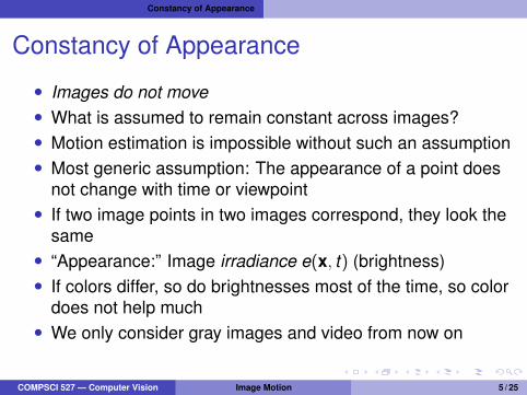
• Make w(x) a (truncated) Gaussian rather than a box
w(x) ∝
{e
12(
‖x‖σ )
2
if |x1| ≤ h and |x2| ≤ h0 otherwise
• Dissimilarity L(xf ,d) =∑
x[g(x + d)− f (x)]2 w(x− xf )depends more on what’s around the window center• Reduces the effects of multiple motions• Does not eliminate them
COMPSCI 527 — Computer Vision Image Motion 17 / 25
The Lucas-Kanade Tracker
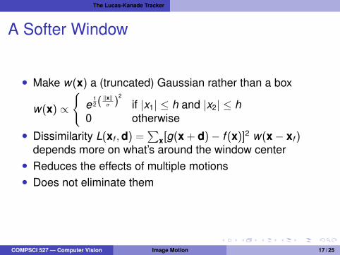
How to Minimize L(xf ,d)?• Method 1: Exhaustive search over a grid of d• Advantages: Unlikely to be trapped in local minima
• Disadvantage: Fixed resolution• Accurate motion is sometimes necessary• Using a very fine grid would be very expensive• Exhaustive search may provide a good initialization
COMPSCI 527 — Computer Vision Image Motion 18 / 25
The Lucas-Kanade Tracker
How to Minimize L(xf ,d)?• Method 2: Use a gradient-descent method• Search space has low dimension (d ∈ R2), so we can use
Newton’s method for faster convergence• Compute gradient and Hessian of
L(d) =∑
x[g(x + d)− f (x)]2 w(x− xf )
(omitted xf from arguments of L for simplicity)• Take Newton steps• Technical difficulty: the unknown d appears inside g(x + d),
and computing a Hessian would require computingsecond-order derivatives of an image, which is availableonly through its pixels• Second derivatives of images are very sensitive to noise
COMPSCI 527 — Computer Vision Image Motion 19 / 25

The Lucas-Kanade Tracker
The Lucas-Kanade Tracker, 1981
• Instead of computing the Hessian ofL(d) =
∑x[g(x + d)− f (x)]2 w(x− xf ),
linearize g(x + d) ≈ g(x) + [∇g(x)]T d• This brings d “outside g”• L(d) is now quadratic in d, and we can find a minimum in
closed form by taking the gradient (no Hessian required)• Only differentiate the image once to get ∇g(x)• Since the solution d1 relies on an approximation, we iterate:
Shift g by d1 to make the residual d smaller, and repeat• This method works for losses that are sums of squares, and
is called the Newton-Raphson method
COMPSCI 527 — Computer Vision Image Motion 20 / 25

The Lucas-Kanade Tracker
Lucas-Kanade Overall Scheme
• Initialize: d0 = 0
• Find a displacement s1 by minimizing linearized L(d0 + s)• Shift g by s1 to obtain g1
• Accumulate: d1 = d0 + s1
• Find a displacement s2 by minimizing linearized L(d1 + s)• Shift g1 by s2 to obtain g2
• Accumulate: d2 = d1 + s2
• . . .
COMPSCI 527 — Computer Vision Image Motion 21 / 25

The Lucas-Kanade Tracker
Lucas-Kanade Derivation• Let dt = s1 + . . .+ st (accumulated shifts, initially 0)
• Let gt(x)def= g(x + dt)
• We seek dt+1 = dt + s by minimizing the following over sL(dt + s) =
∑x[gt(x + s)− f (x)]2 w(x− xf )
with linearization gt(x + s) ≈ gt(x) + [∇gt(x)]T s, so that
L(dt + s) =∑
x
[gt(x + s)− f (x)]2 w(x− xf )
≈∑
x
[gt(x) + [∇gt(x)]T s− f (x)]2 w(x− xf ) ,
a quadratic function of s
COMPSCI 527 — Computer Vision Image Motion 22 / 25

The Lucas-Kanade Tracker
Lucas-Kanade Derivation, Cont’d• Gradient of
L(dt + s) ≈∑
x[gt(x) + [∇gt(x)]T s− f (x)]2 w(x− xf ) is∇L(dt+s) ≈ 2
∑x∇gt(x){gt(x)+[∇gt(x)]T s−f (x)} w(x−xf )
• Setting to zero yields
COMPSCI 527 — Computer Vision Image Motion 23 / 25

The Lucas-Kanade Tracker
The Core System of Lucas-KanadeLinear, 2× 2 system
As = b
whereA =
∑x
∇gt(x)[∇gt(x)]T w(x− xf )
andb =
∑x
∇gt(x)[f (x)− gt(x)] w(x− xf ) .
• Solution yields st (real-valued)• Shift image gt is by st by bilinear interpolation→ gt+1
• Accumulate shifts dt+1 = dt + st (gt+1 is g shifted by dt )• This shift makes f and gt more similar within the windows• Repeat until convergence. Final dt is the answer
COMPSCI 527 — Computer Vision Image Motion 24 / 25

The Lucas-Kanade Tracker
If Motion is Large, Track in a Pyramid
• A large motion at fine level is small at coarse level• (Only drawing one frame per level, for simplicity)• Start at the coarsest level (same window size at all levels)• Multiply solution d by 2 to initialize tracking at the next level• Motion is progressively refined at every level
COMPSCI 527 — Computer Vision Image Motion 25 / 25