1

Image Filtering

Image filtering is used to:

�Remove noise

�Sharpen contrast�Highlight contours

�Detect edges

�Other uses?

Image filters can be classified as linear or nonlinear.Linear filters are also know as convolution filters as they can be

represented using a matrix multiplication.

Thresholding and image equalisation are examples of nonlinear operations, as is the median filter.

2

Median Filtering

Median filtering is a nonlinear method used to remove noise fromimages.

It is widely used as it is very effective at removing noise while preserving edges.

It is particularly effective at removing ‘salt and pepper’ type noise.

The median filter works by moving through the image pixel by pixel, replacing each value with the median value of neighbouring pixels.

The pattern of neighbours is called the "window", which slides, pixel by pixel, over the entire image.

The median is calculated by first sorting all the pixel values from the window into numerical order, and then replacing the pixel being considered with the middle (median) pixel value.

3

Median Filtering exampleThe following example shows the application of a median filter to a simple

one dimensional signal. A window size of three is used, with one entry immediately preceding and

following each entry.Window for x[6]→y[6]

x =

y[0] = median[3 3 9] = 3 y[5] = median[3 6 8] = 6y[1] = median[3 4 9] = 4 y[6] = median[2 6 8] = 6y[2] = median[4 9 52] = 9 y[7] = median[2 2 6] = 2y[3] = median[3 4 52] = 4 y[8] = median[2 2 9] = 2y[4] = median[3 8 52] = 8 y[9] = median[2 9 9] = 9

y =

For y[1] and y[9], extend the left-most or right most value outside theboundaries of the image

same as leaving left-most or right most value unchanged after 1-D median

3 9 4 52 3 8 6 2 2 9

3 4 9 4 8 6 6 2 2 9

93

4

Median Filtering

In the previous example, because there is no entry preceding the first value, the first value is repeated (as is the last value) to obtain enough entries to fill the window.

What effect does this have on the boundary values?

There are other approaches that have different properties that might be preferred in particular circumstances:– Avoid processing the boundaries, with or without cropping the signal or

image boundary afterwards. – Fetching entries from other places in the signal. With images for

example, entries from the far horizontal or vertical boundary might be selected.

– Shrinking the window near the boundaries, so that every window is full.

What effects might these approaches have on the boundary values?

5

Median FilteringOn the left is an image containing a significant amount of salt and

pepper noise. On the right is the same image after processing with a median filter.

Notice the well preserved edges in the image.

There is some remaining noise on the boundary of the image. Why is this?

6

Median Filtering example 22D Median filtering example using a 3 x 3 sampling window:

Keeping border values unchanged

0 2 2

1 2 5

2 3 0

1 2 1

2 5 3

1 1 4

1 3 1

2 2 3

0 1 0

1 4 0

2 2 4

1 0 1

1 1 2

2 2 5

2 3 0

1 1 1

2 2 2

1 1 4

1 3 1

1 1 3

1 2 0

1 4 0

2 1

1 1 1

Input Output

Sorted: 0,0,1,1,1,2,2,4,4

1

7

Median Filtering - Boundaries2D Median filtering example using a 3 x 3 sampling window:Extending border values outside with values at boundary

0 2 2

1 2 5

2 3 0

1 2 1

2 5 3

1 1 4

1 3 1

2 2 3

0 1 0

1 4 0

2 2 4

1 0 1

1 1 2

2 2 2

3 2 2

1 1 1

1 2 2

1 2 2

2 2 2

1 1 1

1 2 2

2 2 2

1 1

1 1 1

Input

Output

Sorted: 0,0,1,1,1,2,2,4,4

1

1

1

3

0

2

5

0

0

1

1

2

1

1

2

1

1

1 4 0 1 3 1

1 1 4 2 3 0

8

Median Filtering - Boundaries2D Median filtering example using a 3 x 3 sampling window:Extending border values outside with 0s

0 2 2

1 2 5

2 3 0

1 2 1

2 5 3

1 1 4

1 3 1

2 2 3

0 1 0

1 4 0

2 2 4

1 0 1

1 1 1

2 2 2

1 1 0

0 1 1

1 2 2

0 1 1

1 1 0

1 1 1

1 2 1

0 2 1

0 1

0 1 1

Input

Output

Sorted: 0,0,1,1,1,2,2,4,4

1

0

0

0

0

0

0

0

0

0

0

0

0

0

0

0

0

0 0 0 0 0 0

0 0 0 0 0 0

9

Average Filtering

Average (or mean) filtering is a method of ‘smoothing’ images by reducing the amount of intensity variation between neighbouring pixels.

The average filter works by moving through the image pixel by pixel, replacing each value with the average value of neighbouring pixels, including itself.

There are some potential problems:� A single pixel with a very unrepresentative value can significantly

affect the average value of all the pixels in its neighbourhood.

� When the filter neighbourhood straddles an edge, the filter willinterpolate new values for pixels on the edge and so will blur that edge. This may be a problem if sharp edges are required in the output.

10

Average FilteringThe following example shows the application of an average filter to a

simple one dimensional signal. A window size of three is used, with one entry immediately preceding

and following each entry.

Window for x[4]→y[4]

x=

y[0] = round((3+3+9)/3)= 5 y[5] = round((3+8+6)/3)= 6y[1] = round((3+9+4)/3)= 5 y[6] = round((8+6+2)/3)= 5 y[2] = round((9+4+52)/3)= 22 y[7] = round((6+2+2)/3)= 3y[3] = round((4+52+3)/3)= 20 y[8] = round((2+2+9)/3)= 4y[4] = round((52+3+8)/3)= 21 y[9] = round((2+9+9)/3)= 7

y=

3 9 4 52 3 8 6 2 2 9

5 5 22 20 21 6 5 3 4 7

For y[1] and y[9], extend the left-most or right most value outside the boundaries of the image

93

11

Filter Comparison

0

10

20

30

40

50

60

Original Signal

Median Filter

Average Filter

The graph above shows the 1D signals from the median and averagefilter examples.

What are the differences in the way the filters have modified the original signal?

12

3 by 3 Average filtering

• Consider the following 3 by 3 average filter:• We can write it mathematically as:

• Why normalizing is important ?

• To keep the image pixel values between 0 and 255

1 1

1 1

1 1

1 11 1

1 1

_ ( , ) 1 _ ( , )

1_ _ ( , ) 1 _ ( , )

1

j i

j i

j i

I new x y I old x i y j

I new normalized x y I old x i y j

= − = −

= − =−

= − =−

= × + +

= × + +

∑ ∑

∑ ∑∑ ∑

1 1 1

1 1 1

1 1 1

13

Average Filtering example 22D Average filtering example using a 3 x 3 sampling window:

Keeping border values unchanged

0 2 2

1 2 5

2 3 0

1 2 1

2 5 3

1 1 4

1 3 1

2 2 3

0 1 0

1 4 0

2 2 4

1 0 1

1 1 2

2 2 5

2 3 0

1 2 1

2 2 2

1 1 4

1 3 1

2 1 3

1 1 0

1 4 0

2 2

1 2 1

Input Output

Average = round(1+4+0+2+2+4+1+0+1)/9 = 2

2

14

Average Filtering - Boundaries2D Average filtering example using a 3 x 3 sampling window:Extending border values outside with values at boundary

0 2 2

1 2 5

2 3 0

1 2 1

2 5 3

1 1 4

1 3 1

2 2 3

0 1 0

1 4 0

2 2 4

1 0 1

1 1 2

2 2 2

3 2 2

2 2 1

2 2 2

2 2 3

2 2 2

2 1 2

1 1 2

2 2 2

2 2 2

1 2 1

Input

Output1

1

3

0

2

5

0

0

1

1

2

1

1

2

1

1

1 4 0 1 3 1

1 1 4 2 3 0

Average = round(1+4+0+1+4+0+2+2+4)/9 = 2

15

Average Filtering - Boundaries2D Median filtering example using a 3 x 3 sampling window:Extending border values outside with 0s (Zero-padding)

0 2 2

1 2 5

2 3 0

1 2 1

2 5 3

1 1 4

1 3 1

2 2 3

0 1 0

1 4 0

2 2 4

1 0 1

1 1 1

2 2 2

2 1 1

1 2 1

1 2 2

1 2 2

1 1 1

2 1 1

1 1 1

1 1 1

1 2 2

1 2 1

Input

Output0

0

0

0

0

0

0

0

0

0

0

0

0

0

0

0

0 0 0 0 0 0

0 0 0 0 0 0

Average = round(2+5+0+3+0+0+0+0+0)/9 = 1

16

Average FilteringOn the left is an image containing a significant amount of salt and

pepper noise. On the right is the same image after processing with an Average filter.

What are the differences in the result compared with the Median filter?

Is this a linear (convolution) or nonlinear filter?

17

Gaussian FilteringGaussian filtering is used to blur images and remove noise and detail.In one dimension, the Gaussian function is:

Where σ is the standard deviation of the distribution. The distribution is assumed to have a mean of 0.

Shown graphically, we see the familiar bell shaped Gaussian distribution.

Gaussian distribution with mean 0 and σ = 1

2

22

2

1( )

2

x

G x e σ

πσ

−=

Gaussian filtering

• Significant values

18

2 2 2 2

2 2 2 2

0.5/ 2/ 9/4 8/

0.5/ 2/ 9/4 8/

0 1 2 3 4

* ( ) / 0.399 1

( ) / (0) 1

x

G x e e e e

G x G e e e e

σ σ σ σ

σ σ σ σ

σ − − − −

− − − −

0 1 2

( ) 0.399 0.242 0.05

( ) / (0) 1 0.6 0.125

x

G x

G x G

For σ=1:

19

Gaussian FilteringStandard DeviationThe Standard deviation of the Gaussian function plays an important

role in its behaviour.The values located between +/- σ account for 68% of the set, while two

standard deviations from the mean (blue and brown) account for 95%, and three standard deviations (blue, brown and green) account for 99.7%.

This is very important when designing a Gaussian kernel of fixedlength.

Distribution of the Gaussian function values (Wikipedia)

20

Gaussian FilteringThe Gaussian function is used in numerous research areas:

– It defines a probability distribution for noise or data.

– It is a smoothing operator.

– It is used in mathematics.

The Gaussian function has important properties which are verified with respect to its integral:

In probabilistic terms, it describes 100% of the possible values of any given space when varying from negative to positive values

Gauss function is never equal to zero.

It is a symmetric function.

( )2exp xI dx π∞

−∞

= − =∫

21

Gaussian Filtering

When working with images we need to use the two dimensional Gaussian function.

This is simply the product of two 1D Gaussian functions (one for each direction) and is given by:

A graphical representation of the 2D

Gaussian distribution with mean(0,0)and σ = 1 is shown to the right.

2 2

222

1( , )

2

x y

G x y e σ

πσ

+−=

22

Gaussian Filtering

The Gaussian filter works by using the 2D distribution as a point-spread function.

This is achieved by convolving the 2D Gaussian distribution function with the image.

We need to produce a discrete approximation to the Gaussian function.This theoretically requires an infinitely large convolution kernel, as the

Gaussian distribution is non-zero everywhere.

Fortunately the distribution has approached very close to zero at about three standard deviations from the mean. 99% of the distributionfalls within 3 standard deviations.

This means we can normally limit the kernel size to contain only values within three standard deviations of the mean.

23

Gaussian Filtering

Gaussian kernel coefficients are sampled from the 2D Gaussian function.

Where σ is the standard deviation of the distribution.

The distribution is assumed to have a mean of zero.

We need to discretize the continuous Gaussian functions to store it as discrete pixels.

An integer valued 5 by 5 convolutionkernel approximating a Gaussian

with a σ of 1 is shown to the right,

2 2

222

1( , )

2

x y

G x y e σ

πσ

+−=

1 4 7 4 1

4 16 26 16 4

7 26 41 26 7

4 16 26 16 4

1 4 7 4 1

1273

24

Gaussian FilteringThe Gaussian filter is a non-uniform low pass filter.

The kernel coefficients diminish with increasing distance from the kernel’s centre.

Central pixels have a higher weighting than those on the periphery.

Larger values of σ produce a wider peak (greater blurring).

Kernel size must increase with increasing σ to maintain the Gaussian nature of the filter.

Gaussian kernel coefficients depend on the value of σ.

At the edge of the mask, coefficients must be close to 0.

The kernel is rotationally symmetric with no directional bias.

Gaussian kernel is separable, which allows fast computation.

Gaussian filters might not preserve image brightness.

25

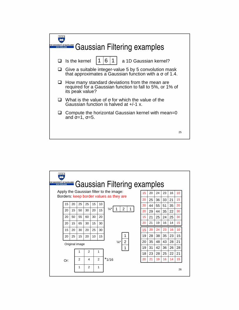
Gaussian Filtering examples

� Is the kernel a 1D Gaussian kernel?

� Give a suitable integer-value 5 by 5 convolution mask that approximates a Gaussian function with a σ of 1.4.

� How many standard deviations from the mean are required for a Gaussian function to fall to 5%, or 1% of its peak value?

� What is the value of σ for which the value of the Gaussian function is halved at +/-1 x.

� Compute the horizontal Gaussian kernel with mean=0 and σ=1, σ=5.

1 6 1

26

Gaussian Filtering examples

15 20 24 23 16 10

19 28 38 35 23 15

20 35 48 43 28 21

19 31 42 36 26 28

18 23 28 25 22 21

20 21 19 16 14 15

15 20 25 25 15 10

20 15 50 30 20 15

20 50 55 60 30 20

20 15 65 30 15 30

15 20 30 20 25 30

20 25 15 20 10 15

15 20 24 23 16 10

20 25 36 33 21 15

20 44 55 51 35 20

20 29 44 35 22 30

15 21 25 24 25 30

20 21 19 16 14 15

1 2 1

1

2

11 2 1

2 4 2

1 2 1

Apply the Gaussian filter to the image:Borders: keep border values as they are

Original image

*1/16Or:

¼*

¼*

27

Gaussian Filtering examples

15 20 25 25 15 10

20 15 50 30 20 15

20 50 55 60 30 20

20 15 65 30 15 30

15 20 30 20 25 30

20 25 15 20 10 15

12 14 25 21 13 9

18 24 43 35 20 15

20 30 54 41 23 21

19 26 51 35 21 26

17 21 35 24 18 24

13 16 17 15 11 15

Original image

10 16 20 19 14 8

15 27 34 32 23 13

18 33 42 38 27 16

17 30 38 35 26 17

14 23 27 25 21 15

10 15 16 15 13 10

Convolve the Gaussian filter (µ=0, σ=1, 0 padding) to the image:

15851

σ=1 means the Gaussian function is at 0 at +/-3σ(g(3)=0.004 and g(0)=0.399, g(1)=0.242, g(2)=0.054). We can approximate a Gaussian function with a kernel of width 5:

1

5

8

5

1

/20

/20

28

Gaussian Filtering examples

15 20 25 25 15 10

20 15 50 30 20 15

20 50 55 60 30 20

20 15 65 30 15 30

15 20 30 20 25 30

20 25 15 20 10 15

15 20 25 25 15 10

20 15 50 30 20 15

20 50 55 60 30 20

20 15 65 30 15 30

15 20 30 20 25 30

20 25 15 20 10 15

Original image

15 20 25 25 15 10

20 15 50 30 20 15

20 50 55 60 30 20

20 15 65 30 15 30

15 20 30 20 25 30

20 25 15 20 10 15

Convolve the Gaussian filter (µ=0, σ=0.2)to the image:

0 1 0

0

1

0σ=0.2 means the Gaussian function is at 0 at +/-3σ(g(0.6)= 0.02 and g(0)= 1.99, g(1)=0.0000074). We can approximate a Gaussian function with a kernel of width 1:

29

Gaussian Filtering

Gaussian filtering is used to remove noise and detail. It is notparticularly effective at removing salt and pepper noise.

Compare the results below with those achieved by the median filter.

30

Gaussian FilteringGaussian filtering is more effective at smoothing images. It has its basis

in the human visual perception system. It has been found that neurons create a similar filter when processing visual images.

The halftone image at left has been smoothed with a Gaussian filter and is displayed to the right.

31

Gaussian Filtering

This is a common first step in edge detection.

The images below have been processed with a Sobel filter commonly used in edge detection applications. The image to the right has had a Gaussian filter applied prior to processing.

32

ConvolutionThe convolution of two functions f and g is defined as:

Where is a function that represents the image and is a function that represents the kernel.

In practice, the kernel is only defined over a finite set of points, so we can modify the definition to:

Where is the width of the kernel and is the height of the kernel.

g is defined only over the points .

( * )( , ) ( , ) ( , )v u

f g x y f u v g x u y v∞ ∞

=−∞ =−∞

= − −∑ ∑

( , )f x y ( , )g x y

( * )( , ) ( , ) ( , )y h x w

v y h u x w

f g x y f u v g x u y v+ +

= − = −

= − −∑ ∑

2 1w + 2 1h +

[ , ] [ , ]w w h h− × −

33

3 by 3 convolution

• Consider the above 3 by 3 kernel with weights .• We can write the convolution Image I_old by the above kernel as:

Why normalizing is important ?

1 1

1 1

1 1

1 11 1

1 1

_ ( , ) _ ( , )

1_ _ ( , ) _ ( , )

ijj i

ijj i

ijj i

I new x y I old x i y j

I new normalized x y I old x i y j

α

αα

= − =−

= − = −

=− = −

= − −

= − −

∑ ∑

∑ ∑∑ ∑

11 01 11

10 00 10

1 1 0 1 1 1

α α αα α αα α α

−

−

− − − −

1

0

-1

-1 0 1

Kernel axis

x→

y ↑

ijα

If all are positive we can normalise the kernel.ijα

34

Convolution Pseudocode

Pseudocode for the convolution of an image f(x,y) with a kernel k(x,y) (2w+1 columns, 2h+1 lines) to produce a new image g(x,y):

for y = 0 to ImageHeight dofor x = 0 to ImageWidth do

sum = 0for i= -h to h do

for j = -w to w dosum = sum + k(j,i) * f(x - j, y - i)

end forend forg(x,y) = sum

end forend for

1

0

-1

-1 0 1

Kernel axis

Convolution equation for a 3 by 3 kernelThe pixel value p(x,y) of image f after convolution with a 3 by 3

kernel k is:

35

1

0

-1

-1 0 1

Kernel k

x→

y ↑( 1,1) (0,1) (1,1)

( 1,0) (0,0) (1,0)

( 1, 1) (0, 1) (1, 1)

k k k

k k k

k k k

−

−

− − − −

11

1 1

( , ) ( , ) ( , )

( 1, 1) ( 1, 1)

(0, 1) ( , 1)

(1, 1) ( 1, 1)

( 1,0) ( 1, )

(0,0) ( , )

(1,0) ( 1, )

ji

i j

p x y k j i f x j y i

k f x y

k f x y

k f x y

k f x y

k f x y

k f x y

=+=+

=− =−

= − −

= − − + + += − + += − − + += − + += += − +

∑∑

( 1,1) ( 1, 1)

(0,1) ( , 1)

(1,1) ( 1, 1)

k f x y

k f x y

k f x y

= − + − += − += − −

36

Convolution examples

15 20 25 25 15 10

20 15 50 30 20 15

20 50 55 60 30 20

20 15 65 30 15 30

15 20 30 20 25 30

20 25 15 20 10 15

55

Original image

Do the convolution of the following kernel k with the image I:

x

y

1 0 -1

0 1 0

-1 0 1

1

0

-1

-1 0 1

Kernel

P(x,y)= -1*30+0*50+1*15+0*60+1*55+0*50+1*30+0*65+

-1*15= 55

k*I

37

Convolution – Potential Problems

Summation over a neighbourhood might exceed the range and/or sign permitted in the image format:

– The data may need to be temporarily stored in a 16 – 32 bit integer representation.

– Then normalised back to the appropriate range (0-255 for an 8 bit image).

Another issue is how to deal with image borders:

– Convolution is not possible if part of the kernel lies outside the image.

– What is the size of image window which is processed normally when performing a Convolution of size m x n on an original image of size M x N ?

38

Convolution Border IssuesHow to deal with convolution at image borders:1) Extend image limits with 0s (Zero padding)2) Extend image limits with own image values3) Generate specific filters to take care of the borders

Find the corner and border specific kernel for:

1 1 1

1 1 1

1 1 1

-1 -1 -1

-1 8 -1

-1 -1 -1

-1 0 1

-1 0 1

-1 0 1

Image top leftcorner filter:

1 1

1 1

Kernel center (in red)

Image left most column filter:

Kernel center (in red)

-1 -1

-1 5

-1 -1

Top row filter:

Kernel center (in red)

-1 0 1

39

Edge Detection

Edges in images are areas with strong intensity contrasts; a jump in intensity from one pixel to the next.

The process of edge detection significantly reduces the amount of data and filters out unneeded information, while preserving the important structural properties of an image.

There are many different edge detection methods, the majority of which can be grouped into two categories:

�Gradient, �and Laplacian.

The gradient method detects the edges by looking for the maximumand minimum in the first derivative of the image.

The Laplacian method searches for zero crossings in the second derivative of the image .

We will look at two examples of the gradient method, Sobel and Prewitt.

40

Edge Detection

Edge detection is a major application for convolution.What is an edge:

• A location in the image where is a sudden change in the intensity/colour of pixels.

• A transition between objects or object and background.• From a human visual perception perspective it attracts attention.

Problem: Images contain noise, which also generates sudden transitions of pixel values.

Usually there are three steps in the edge detection process:1) Noise reduction

Suppress as much noise as possible without removing edges.2) Edge enhancement

Highlight edges and weaken elsewhere (high pass filter).3) Edge localisation

Look at possible edges (maxima of output from previous filter) and eliminate spurious edges (often noise related).

41

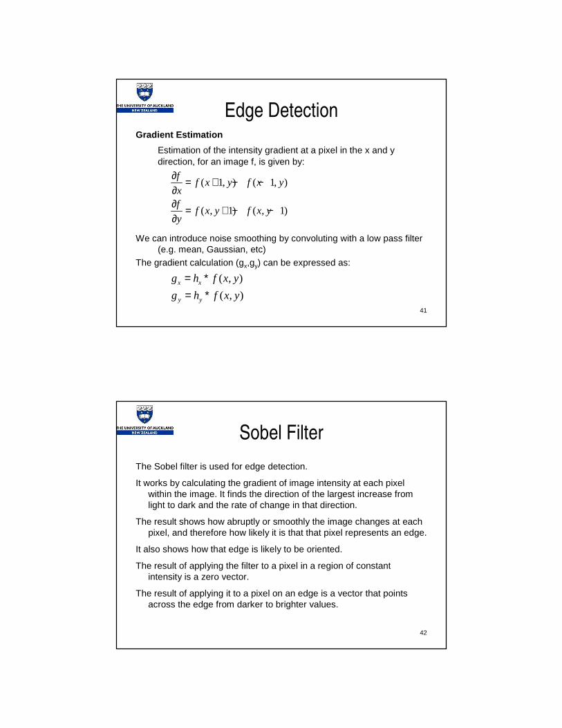
Edge DetectionGradient Estimation

Estimation of the intensity gradient at a pixel in the x and y direction, for an image f, is given by:

We can introduce noise smoothing by convoluting with a low pass filter (e.g. mean, Gaussian, etc)

The gradient calculation (gx,gy) can be expressed as:

( 1, ) ( 1, )

( , 1) ( , 1)

ff x y f x y

xf

f x y f x yy

∂ = + − −∂∂ = + − −∂

( , )

( , )x x

y y

g h f x y

g h f x y

= ∗= ∗

42

Sobel Filter

The Sobel filter is used for edge detection.

It works by calculating the gradient of image intensity at each pixel within the image. It finds the direction of the largest increase from light to dark and the rate of change in that direction.

The result shows how abruptly or smoothly the image changes at each pixel, and therefore how likely it is that that pixel represents an edge.

It also shows how that edge is likely to be oriented.

The result of applying the filter to a pixel in a region of constant intensity is a zero vector.

The result of applying it to a pixel on an edge is a vector that points across the edge from darker to brighter values.

43

Sobel FilterThe sobel filter uses two 3 x 3 kernels. One for changes in the

horizontal direction, and one for changes in the vertical direction.The two kernels are convolved with the original image to calculate the

approximations of the derivatives.If we define Gx and Gy as two images that contain the horizontal and

vertical derivative approximations respectively, the computations are:

and

Where A is the original source image.

The x coordinate is defined as increasing in the right-direction and the y coordinate is defined as increasing in the down-direction.

1 2 1

0 0 0

1 2 1yG A

− − − = ∗

1 0 1

2 0 2

1 0 1xG A

−

−

−

= ∗

44

Sobel Filter

To compute Gx and Gy we move the appropriate kernel (window) over the input image, computing the value for one pixel and then shifting one pixel to the right. Once the end of the row is reached, we move down to the beginning of the next row.

The example below shows the calculation of a value of Gx:

kernel =

Input image Output image (Gx)

b22 = a13 - a11 + 2a23 - 2a21 + a33 - a31

b11 b12 b13 …

b21 b22 b23 …

b31 b32 b33 …

… … … …

a11 a12 a13 …

a21 a22 a23 …

a31 a32 a33 …

… … … …

1 0 -1

2 0 -2

1 0 -1

45

Edge DetectionThe kernels contain positive and negative coefficients.

This means the output image will contain positive and negative values.

For display purposes we can:

• map the gradient of zero onto a half-tone grey level.

– This makes negative gradients appear darker, and positive gradients appear brighter.

• Use the absolute values of the gradient map (stretched between 0and 255).

• This makes very negative and very positive gradients appear brighter.

The kernels are sensitive to horizontal and vertical transitions.

The measure of an edge is its amplitude and angle. These are readily calculated from Gx and Gy.

46

Sobel Filter

At each pixel in the image, the gradient approximations given by Gx and Gy are combined to give the gradient magnitude, using:

The gradient’s direction is calculated using:

A value of 0 would indicate a vertical edge that is darker on the left side.

2 2x yG G G= +

arctan y

x

G

G

Θ =

Θ

47

Sobel Filter

1 0 1

2 0 2

1 0 1xG A

−

−

−

= ∗

The image to the right above is Gx, calculated as:Where A is the original image to the left.

Notice the general orientation of the edges.What would you expect to be different in Gy?

48

Sobel Filter

The image to the right above is Gy, calculated as:

Where A is the original image to the left.

What do we expect from the combined image?

1 2 1

0 0 0

1 2 1yG A

− − − = ∗

49

Sobel Filter

The image to the right above is the result of combining the Gx and Gy

derivative approximations calculated from image A on the left.

50

Sobel Filter example

10 50 10 50 10

10 55 10 55 10

10 65 10 65 10

10 50 10 50 10

10 55 10 55 10

Original image

-1 -2 -1

0 0 0

1 2 1

Convolve the Sobel kernels to the original image (use 0 padding)

155 0 0 0 -155

225 0 0 0 -225

235 0 0 0 -235

220 0 0 0 -220

160 0 0 0 -160

-75 -130 -130 -130 -75

-15 -30 -10 -30 -15

5 10 10 10 5

10 20 20 20 10

70 120 120 120 70

1 0 -1

2 0 -2

1 0 -1

51

Sobel filter example• Compute Gx and Gy, gradients of the image performing the

convolution of Sobel kernels with the image• Use zero-padding to extend the image

0 0 10 10 10

0 0 10 10 10

0 0 10 10 10

0 0 10 10 10

0 0 10 10 10

x

y

1 0 -1

2 0 -2

1 0 -1

0 30 30 0 -30

0 40 40 0 -40

0 40 40 0 -40

0 40 40 0 -40

0 30 30 0 -30

-10 -30 -40 -30 -10

0 0 0 0 0

0 0 0 0 0

0 0 0 0 0

10 30 40 30 10

-1 -2 -1

0 0 0

1 2 1

hx hy

Gx

Gy

52

Sobel filter example• Compute Gx and Gy, gradients of the image performing the

convolution of Sobel kernels with the image• Use border values to extend the image

0 0 10 10 10

0 0 10 10 10

0 0 10 10 10

0 0 10 10 10

0 0 10 10 10

x

y

1 0 -1

2 0 -2

1 0 -1

0 40 40 0 0

0 40 40 0 0

0 40 40 0 0

0 40 40 0 0

0 40 40 0 0

0 0 0 0 0

0 0 0 0 0

0 0 0 0 0

0 0 0 0 0

0 0 0 0 0

-1 -2 -1

0 0 0

1 2 1

hx hy

Gx

Gy

0 0

0 0

0 0

0 0

0 0

arctan y

x

G

G

Θ =

53

Sobel filter example• Compute Gx and Gy, gradients of the image performing the

convolution of Sobel kernels with the image• Use border values to extend the image

0 0 0 0 0

0 0 0 0 0

10 10 10 10 10

10 10 10 10 10

10 10 10 10 10

x

y

1 0 -1

2 0 -2

1 0 -1

0 0 0 0 0

0 0 0 0 0

0 0 0 0 0

0 0 0 0 0

0 0 0 0 0

0 0 0 0 0

-40 -40 -40 -40 -40

-40 -40 -40 -40 -40

0 0 0 0 0

0 0 0 0 0

-1 -2 -1

0 0 0

1 2 1

hx hy

Gx

Gy

-∞ -∞ -∞ -∞ -∞

-∞ -∞ -∞ -∞ -∞arctan y

x

G

G

Θ =

54

Prewitt Filter

The Prewitt filter is similar to the Sobel in that it uses two 3 x 3 kernels. One for changes in the horizontal direction, and one for changes in the vertical direction.

The two kernels are convolved with the original image to calculate the approximations of the derivatives.

If we define Gx and Gy as two images that contain the horizontal and vertical derivative approximations respectively, the computations are:

and

Where A is the original source image.

The x coordinate is defined as increasing in the right-direction and the y coordinate is defined as increasing in the down-direction.

1 0 1

1 0 1

1 0 1xG A

−−

−

= ∗

1 1 1

0 0 0

1 1 1

*yG A

− − − =

55

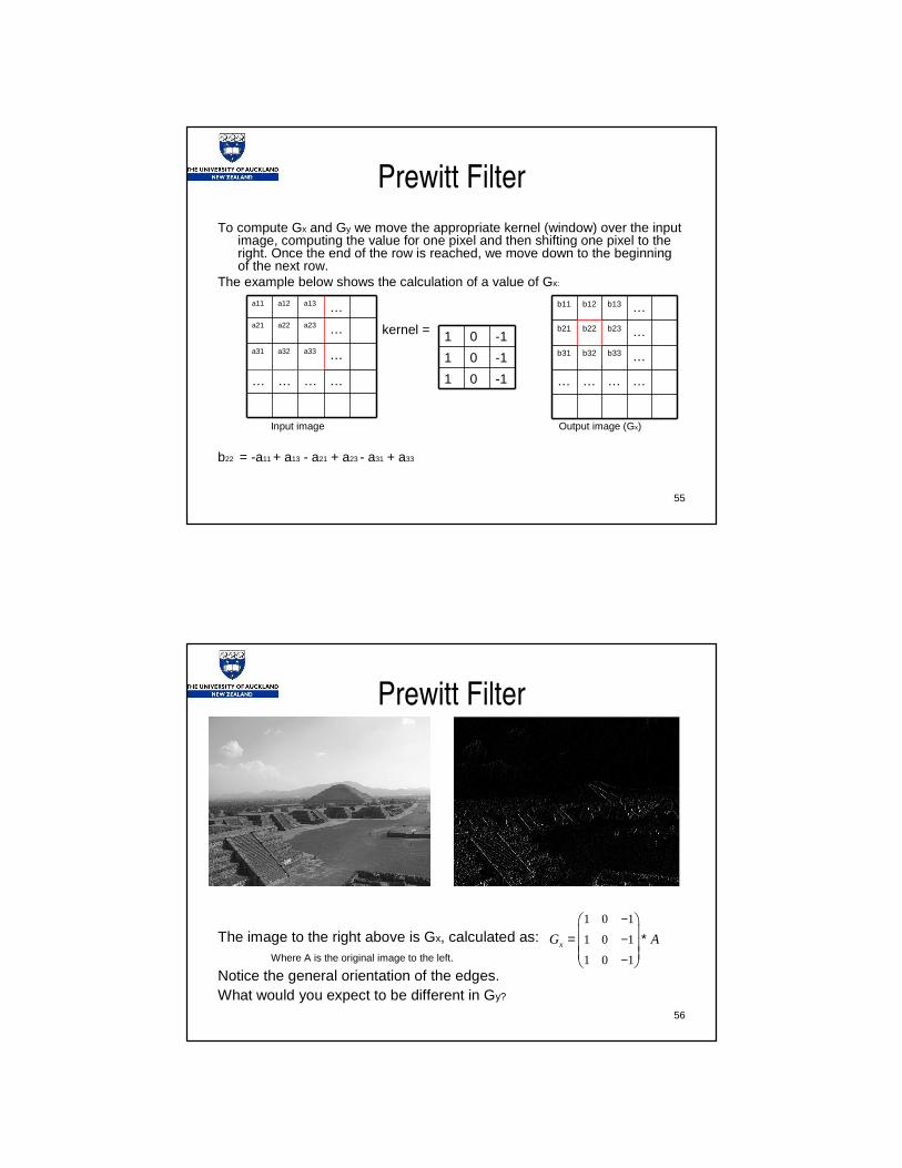
Prewitt Filter

To compute Gx and Gy we move the appropriate kernel (window) over the input image, computing the value for one pixel and then shifting one pixel to the right. Once the end of the row is reached, we move down to the beginning of the next row.

The example below shows the calculation of a value of Gx:

kernel =

Input image Output image (Gx)

b22 = -a11 + a13 - a21 + a23 - a31 + a33

b11 b12 b13 …

b21 b22 b23 …

b31 b32 b33 …

… … … …

a11 a12 a13 …a21 a22 a23 …

a31 a32 a33 …

… … … …

1 0 -1

1 0 -1

1 0 -1

56

Prewitt Filter

The image to the right above is Gx, calculated as:Where A is the original image to the left.

Notice the general orientation of the edges.What would you expect to be different in Gy?

1 0 1

1 0 1

1 0 1xG A

−

−

−

= ∗

57

Prewitt Filter

The image to the right above is Gy, calculated as:

Where A is the original image to the left.

What do we expect from the combined image?

1 1 1

0 0 0

1 1 1

*yG A

− − − =

58

Prewitt Filter

The image to the right above is the result of combining the Gx and Gy

derivative approximations calculated from image A on the left.

59

Prewitt Filter example

10 50 10 50 10

10 55 10 55 10

10 65 10 65 10

10 50 10 50 10

10 55 10 55 10

Original image

-1 -1 -1

0 0 0

1 1 1

Convolve the Prewitt kernels to the original image (0 padding)

105 0 0 0 -105

170 0 0 0 -170

170 0 0 0 -170

170 0 0 0 -170

105 0 0 0 -105

-65 -75 -120 -75 -65

-15 -15 -30 -15 -15

5 5 10 5 5

10 10 20 10 10

50 70 110 75 65

1 0 -1

1 0 -1

1 0 -1

60

Laplacian filter example• Compute the convolution of the Laplacian kernels L_4 and

L_8 with the image• Use border values to extend the image

0 0 10 10 10

0 0 10 10 10

0 0 10 10 10

0 0 10 10 10

0 0 10 10 10

x

y

-1 -1 -1

-1 8 -1

-1 -1 -1

0 -30 30 0 0

0 -30 30 0 0

0 -30 30 0 0

0 -30 30 0 0

0 -30 30 0 0

0 -10 10 0 0

0 -10 10 0 0

0 -10 10 0 0

0 -10 10 0 0

0 -10 10 0 0

L_8

L_8

L_4

0 -1 0

-1 4 -1

0 -1 0

L_4

61

Laplacian filter example• Compute the convolution of the Laplacian kernels L_4 and

L_8 with the image• Use zero-padding to extend the image

0 0 10 10 10

0 0 10 10 10

0 0 10 10 10

0 0 10 10 10

0 0 10 10 10

x

y

-1 -1 -1

-1 8 -1

-1 -1 -1

0 -20 50 50 50

0 -30 30 0 30

0 -30 30 0 30

0 -30 30 0 30

0 -20 50 50 50

0 -10 20 10 20

0 -10 10 0 10

0 -10 10 0 10

0 -10 10 0 10

0 -10 20 10 20

L_8

L_8

L_4

0 -1 0

-1 4 -1

0 -1 0

L_4