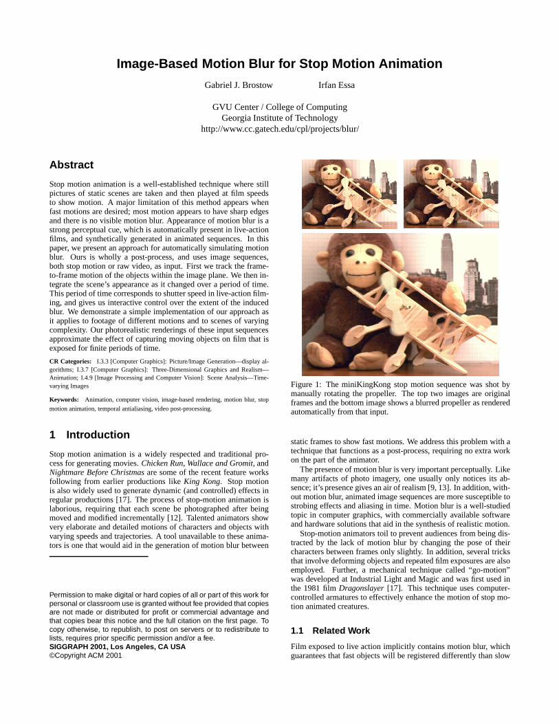
Image-Based Motion Blur for Stop Motion Animation

Gabriel J. Brostow Irfan Essa

GVU Center / College of ComputingGeorgia Institute of Technology

http://www.cc.gatech.edu/cpl/projects/blur/

Abstract

Stop motion animation is a well-established technique where stillpictures of static scenes are taken and then played at film speedsto show motion. A major limitation of this method appears whenfast motions are desired; most motion appears to have sharp edgesand there is no visible motion blur. Appearance of motion blur is astrong perceptual cue, which is automatically present in live-actionfilms, and synthetically generated in animated sequences. In thispaper, we present an approach for automatically simulating motionblur. Ours is wholly a post-process, and uses image sequences,both stop motion or raw video, as input. First we track the frame-to-frame motion of the objects within the image plane. We then in-tegrate the scene’s appearance as it changed over a period of time.This period of time corresponds to shutter speed in live-action film-ing, and gives us interactive control over the extent of the inducedblur. We demonstrate a simple implementation of our approach asit applies to footage of different motions and to scenes of varyingcomplexity. Our photorealistic renderings of these input sequencesapproximate the effect of capturing moving objects on film that isexposed for finite periods of time.

CR Categories: I.3.3 [Computer Graphics]: Picture/Image Generation—display al-gorithms; I.3.7 [Computer Graphics]: Three-Dimensional Graphics and Realism—Animation; I.4.9 [Image Processing and Computer Vision]: Scene Analysis—Time-varying Images

Keywords: Animation, computer vision, image-based rendering, motion blur, stop

motion animation, temporal antialiasing, video post-processing.

1 Introduction

Stop motion animation is a widely respected and traditional pro-cess for generating movies. Chicken Run, Wallace and Gromit, andNightmare Before Christmas are some of the recent feature worksfollowing from earlier productions like King Kong. Stop motionis also widely used to generate dynamic (and controlled) effects inregular productions [17]. The process of stop-motion animation islaborious, requiring that each scene be photographed after beingmoved and modified incrementally [12]. Talented animators showvery elaborate and detailed motions of characters and objects withvarying speeds and trajectories. A tool unavailable to these anima-tors is one that would aid in the generation of motion blur between

Figure 1: The miniKingKong stop motion sequence was shot bymanually rotating the propeller. The top two images are originalframes and the bottom image shows a blurred propeller as renderedautomatically from that input.

static frames to show fast motions. We address this problem with atechnique that functions as a post-process, requiring no extra workon the part of the animator.

The presence of motion blur is very important perceptually. Likemany artifacts of photo imagery, one usually only notices its ab-sence; it’s presence gives an air of realism [9, 13]. In addition, with-out motion blur, animated image sequences are more susceptible tostrobing effects and aliasing in time. Motion blur is a well-studiedtopic in computer graphics, with commercially available softwareand hardware solutions that aid in the synthesis of realistic motion.

Stop-motion animators toil to prevent audiences from being dis-tracted by the lack of motion blur by changing the pose of theircharacters between frames only slightly. In addition, several tricksthat involve deforming objects and repeated film exposures are alsoemployed. Further, a mechanical technique called “go-motion”was developed at Industrial Light and Magic and was first used inthe 1981 film Dragonslayer [17]. This technique uses computer-controlled armatures to effectively enhance the motion of stop mo-tion animated creatures.

1.1 Related Work

Film exposed to live action implicitly contains motion blur, whichguarantees that fast objects will be registered differently than slow

Permission to make digital or hard copies of all or part of this work forpersonal or classroom use is granted without fee provided that copiesare not made or distributed for profit or commercial advantage andthat copies bear this notice and the full citation on the first page. Tocopy otherwise, to republish, to post on servers or to redistribute tolists, requires prior specific permission and/or a fee.SIGGRAPH 2001, Los Angeles, CA USA©Copyright ACM 2001

moving ones. At present, only research in computer animation hasaddressed the problem of creating photorealistic motion blurred im-ages. Antialiasing of time-sampled 3D motion is now a standardpart of most rendering pipelines.

The seminal work in motion blur was first introduced in 1983 byKorein and Badler [11], and Potmesil and Chakravarty [14]. Kor-ein and Badler introduced two approaches, both modeled after tra-ditional cartoonists’ work. The first implementation parameterizedthe motion over time of 2D primitives such as discs. The secondrelied on supersampling the moving image and then filtering theresulting intensity function to generate images with superimposedmultiple renderings of the action. The resulting images look likemultiply exposed film.

Potmesil and Chakravarty proposed a different method for blur-ring motion continuously. A general-purpose camera model accu-mulates (in time) the image-plane sample points of a moving objectto form a path. Each sample’s color values are then convolved withthat path to generate finite-time exposures that are photorealistic.

The most significant subsequent development in antialiasing inthe time domain came with the distributed raytracing work ofCook et al. [6]. This work successfully combines image-space an-tialiasing with a modified supersampling algorithm that retrievespixel values from randomly sampled points in time.

These algorithms cannot be applied directly to raster imagesof stop motion animation because the transformation informationabout the scene is absent. Both convolution with a path and super-sampling that path in time require that the motion be fully speci-fied while the “shutter” is open. Raster images of stop motion areeffectively snapshots, which in terms of motion, were shot withan infinitely fast shutter. While only the animator knows the truepaths of the objects, visual inspection of the scene allows us to in-fer approximations of the intended motion paths. Cucka [7] man-aged to estimate localized motions when developing a system toadd motion blur to hand-drawn animations. Much like the commer-cial blur-generation and video-retiming packages currently avail-able, only small frame-to-frame motions are tracked successfully,and pre-segmentation must be done either by hand or as part of theanimation process.

Our approach is entirely image-based. Animators can adjust theextent of the generated blur to their liking after the images areacquired. We take advantage of well-established computer visiontechniques to segment and track large motions throughout a se-quence. Our proposed techniques rely on combinations of back-ground subtraction and template matching in addition to the previ-ously explored capabilities of optical flow and visual motion com-putations. Though existing techniques for encoding motions arebecoming quite refined (e.g., MPEG-4 [10]), such methods are notsufficient for our needs.

1.2 Overview

We are interested in changing the regions of an image sequencewhich correspond to stop motion activity to show motion blur. Ourgoal is to give the user control over the amount of blur, and to per-form the rest of the process as automatically as possible. One majortask is the detection and extraction of regions that are affected bymovement in consecutive frames.

To help determine the correspondence between pixels in twoconsecutive frames, we initially group neighboring pixels withineach image into blobs, and these are assumed to move indepen-dently (Section 2). The affine transformations of these blobs aretracked and recorded as pixel-specific motion vectors. These vec-tors may subsequently be refined individually to model other typesof motion. Once the motion vectors adequately explain how the pix-els from a previous image move to their new positions in the currentimage, each pixel is blurred (Section 3). The pixel color values are

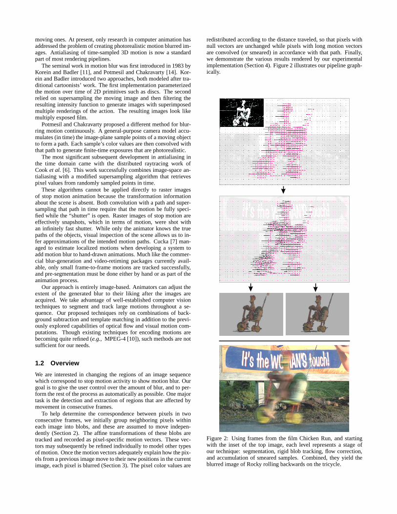
redistributed according to the distance traveled, so that pixels withnull vectors are unchanged while pixels with long motion vectorsare convolved (or smeared) in accordance with that path. Finally,we demonstrate the various results rendered by our experimentalimplementation (Section 4). Figure 2 illustrates our pipeline graph-ically.

Figure 2: Using frames from the film Chicken Run, and startingwith the inset of the top image, each level represents a stage ofour technique: segmentation, rigid blob tracking, flow correction,and accumulation of smeared samples. Combined, they yield theblurred image of Rocky rolling backwards on the tricycle.

2 Finding Pixel Transformations

Ideally, we desire the same 3D transformation data as is availableto mesh-based animation renderers. Some structure-from-motionand scene reconstruction techniques, studied by computer visionresearchers, are capable of extracting such pose information fromcertain classes of image sequences [8]. They usually seek optimalscene geometry assuming that a single motion, like that of the cam-era, caused all the changes in the scene. Footage containing articu-lated characters is troublesome because multiple motions contributeto the changes. Ours is consequently a rather brute-force but gen-eral purpose 2D motion estimation method. The resulting system isbut a variant of the possible motion estimators that could satisfy theneeds of our approach. The following description explains how tohandle objects that are traveling large distances between subsequentframes.

2.1 Scene Segmentation

The task of segmenting and grouping pixels that are tracked is sim-plified by the high quality of the footage captured for most stopmotion animations. Additionally, scenes shot with a moving cam-era tend to be the exception, so background-subtraction is a naturalchoice for segmenting the action.

If a clean background plate is not available, median filtering inthe time domain can usually generate one. We observe a pixel loca-tion over the entire sequence, sorting the intensity values (as manyas there are frames). By choosing the median, the background canbe reconstituted one pixel at a time. This highly parallelizable pro-cess results in choosing the colors which were most frequently sam-pled by a given pixel, or at least colors that were closest to doing so.Given a reasonably good image of the background (Ib), the pixelsthat are different in a given frame (If ) are isolated. An image (Im)containing only pixels that are moving is obtained according to thiscriterion:

Im(x, y) =

�If (x, y) |If (x, y)− Ib(x, y)| > threshold

0 otherwise(1)

A good threshold value, that worked on all sequences we pro-cessed, was 7.8% of the intensity scale’s range. Note that we usegrayscale versions of our color difference images when comparingagainst this threshold. Each contiguous region of pixels within Im

is grouped as a single blob (b), with the intent of locating it againin the subsequent frame. Naturally, blobs representing separate ob-jects can merge and separate over time, depending on their proxim-ity. While this has not been a problem for us, it can be dealt withby using color-similarity and contour-completion as supplementarymeans of chopping the scene into manageable blobs. These futureextensions would also help in dealing with footage shot with a mov-ing camera.

2.2 Blob Tracking

Objects, and therefore the blobs that represent them, can move sig-nificantly between frame i and frame i + 1. To determine the pathsalong which blur will eventually take place, we must first find acorrespondence which maps each blob to its appearance in suc-cessive frames. This motion estimation is a long-standing visionresearch problem. Large regions of solid color and non-uniformscene-lighting compound the violation of the optical flow constraintequation. Hierarchical techniques, some of which include rigid-ity constraints, have been developed to make this problem moretractable. Bergen et al. [1] developed a hierarchical frameworkwhich unifies several parameter-based optical flow methods. These

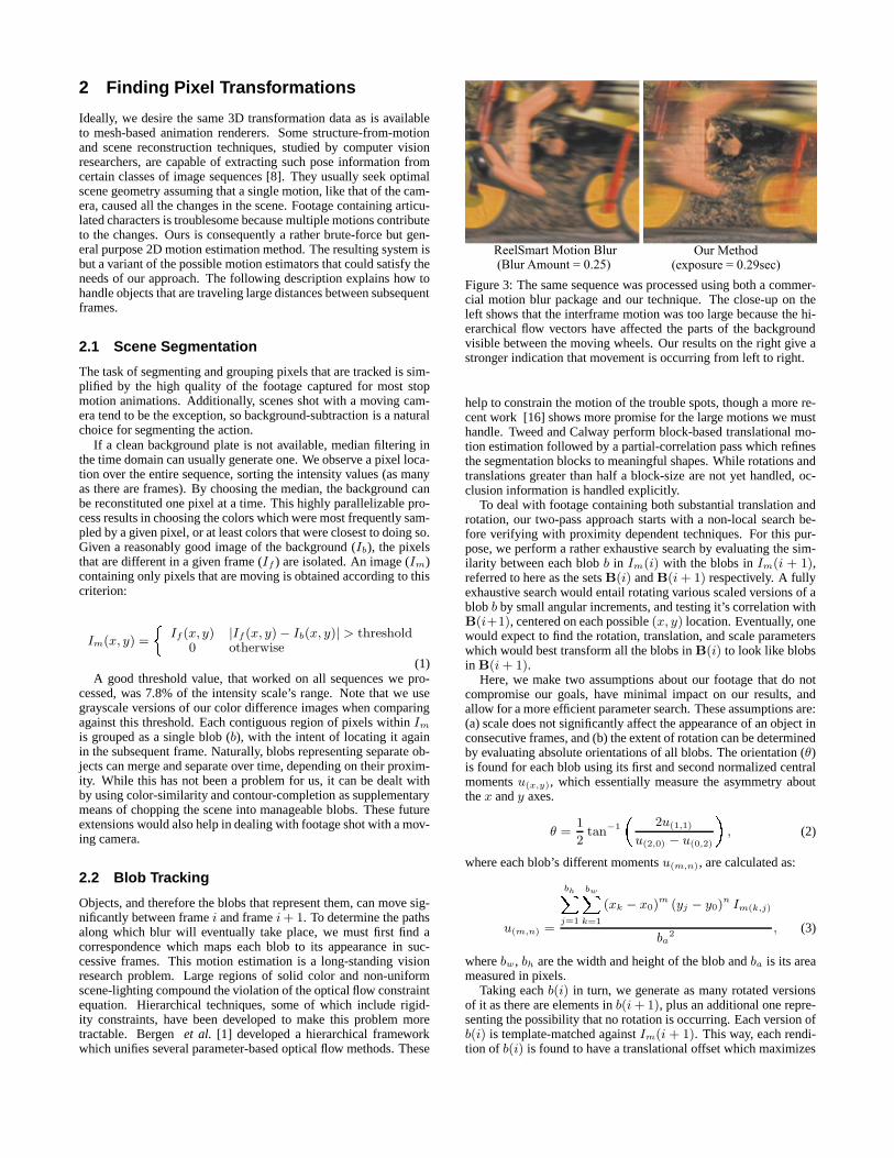
ReelSmart Motion Blur(Blur Amount = 0.25)

Our Method(exposure = 0.29sec)

Figure 3: The same sequence was processed using both a commer-cial motion blur package and our technique. The close-up on theleft shows that the interframe motion was too large because the hi-erarchical flow vectors have affected the parts of the backgroundvisible between the moving wheels. Our results on the right give astronger indication that movement is occurring from left to right.

help to constrain the motion of the trouble spots, though a more re-cent work [16] shows more promise for the large motions we musthandle. Tweed and Calway perform block-based translational mo-tion estimation followed by a partial-correlation pass which refinesthe segmentation blocks to meaningful shapes. While rotations andtranslations greater than half a block-size are not yet handled, oc-clusion information is handled explicitly.

To deal with footage containing both substantial translation androtation, our two-pass approach starts with a non-local search be-fore verifying with proximity dependent techniques. For this pur-pose, we perform a rather exhaustive search by evaluating the sim-ilarity between each blob b in Im(i) with the blobs in Im(i + 1),referred to here as the sets B(i) and B(i + 1) respectively. A fullyexhaustive search would entail rotating various scaled versions of ablob b by small angular increments, and testing it’s correlation withB(i+1), centered on each possible (x, y) location. Eventually, onewould expect to find the rotation, translation, and scale parameterswhich would best transform all the blobs in B(i) to look like blobsin B(i + 1).

Here, we make two assumptions about our footage that do notcompromise our goals, have minimal impact on our results, andallow for a more efficient parameter search. These assumptions are:(a) scale does not significantly affect the appearance of an object inconsecutive frames, and (b) the extent of rotation can be determinedby evaluating absolute orientations of all blobs. The orientation (θ)is found for each blob using its first and second normalized centralmoments u(x,y), which essentially measure the asymmetry aboutthe x and y axes.

θ =1

2tan−1 � 2u(1,1)

u(2,0) − u(0,2) � , (2)

where each blob’s different moments u(m,n), are calculated as:

u(m,n) =

bh�j=1

bw�k=1

(xk − x0)m (yj − y0)

n Im(k,j)

ba2

, (3)

where bw , bh are the width and height of the blob and ba is its areameasured in pixels.

Taking each b(i) in turn, we generate as many rotated versionsof it as there are elements in b(i + 1), plus an additional one repre-senting the possibility that no rotation is occurring. Each version ofb(i) is template-matched against Im(i + 1). This way, each rendi-tion of b(i) is found to have a translational offset which maximizes

the normalized cross correlation (NCC). The normalized correla-tion between a blob’s pixel values, b(x, y), and an image, I(x, y),is calculated at each coordinate as:

NCC =

bh�j=1

bw�k=1

b(k, j) I(x + k, y + j)���� bh�j=1

bw�k=1

b(k, j)2 � bh�j=1

bw�k=1

I(x + k, y + j)2 � . (4)

The version of b(i) which achieves the highest correlation score(usually above 0.9) is recorded as the best estimate of a blob’s mo-tion between frames i and i + 1. It is interesting to note that withobjects entering and leaving the scene, the best translation and ro-tation parameters often push a blob beyond the image boundaries.

2.3 Flow Correction

The current blob tracking results represent the best estimate of therotations and translations performed by the objects in the scene.By applying the respective 2D transformations to each blob’s con-stituent pixel coordinates, a vector map Vi, representing the move-ment of each pixel from its original location is obtained. A currentestimate of If (i+1), called Ir(i+1), is regenerated by applying theVi vectors to If (i). Ideally, Ir(i + 1) would look like If (i + 1)if all the motions were purely due to translation and rotation. Inpractice, other transformations and lighting changes combine withthe effects of perspective projection to reveal that we must locallyrefine the motion estimates. Since there is a large selection of al-gorithms for computing visual motion, we tried several differentones and are now using a slightly modified version of the methodproposed by Black and Anandan [2]. This method computes hier-archical optical flow to find the motion vectors which best warpedIr(i + 1) to look like If (i + 1). The benefits of other local-motionestimation algorithms can be significant, but each has a breakingpoint that can be reached when the frame-to-frame deformation orlighting changes are too large.

Estimating optical flow allows for the creation of a map of cor-rective motion vectors. The map is combined with the initial mo-tion vectors in Vi. Ir(i+1) images regenerated using the correctedVi’s now have fewer visible discrepancies when compared againsttheir intended appearance (see Figure 2).

3 Rendering Blur

The frame-to-frame transformations intended by the animator havenow been approximated. We proceed to interpolate paths alongwhich pixels will be blurred.

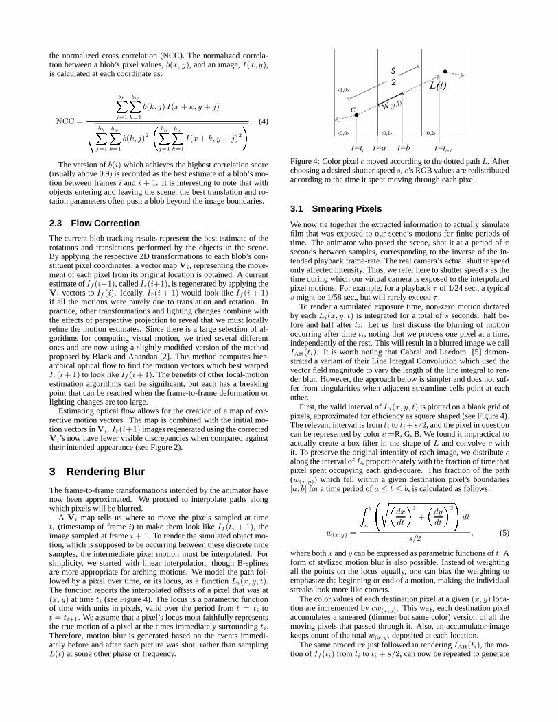
A Vi map tells us where to move the pixels sampled at timeti (timestamp of frame i) to make them look like If (ti + 1), theimage sampled at frame i + 1. To render the simulated object mo-tion, which is supposed to be occurring between these discrete timesamples, the intermediate pixel motion must be interpolated. Forsimplicity, we started with linear interpolation, though B-splinesare more appropriate for arching motions. We model the path fol-lowed by a pixel over time, or its locus, as a function Li(x, y, t).The function reports the interpolated offsets of a pixel that was at(x, y) at time ti (see Figure 4). The locus is a parametric functionof time with units in pixels, valid over the period from t = ti tot = ti+1. We assume that a pixel’s locus most faithfully representsthe true motion of a pixel at the times immediately surrounding ti.Therefore, motion blur is generated based on the events immedi-ately before and after each picture was shot, rather than samplingL(t) at some other phase or frequency.

c

s

2

t=a t=b t=ti+1t=ti

L(t)

w (0 ,1)

‹ ›0,10,0 ‹ ›0,2

‹1 ›,0

‹ ›

Figure 4: Color pixel c moved according to the dotted path L. Afterchoosing a desired shutter speed s, c’s RGB values are redistributedaccording to the time it spent moving through each pixel.

3.1 Smearing Pixels

We now tie together the extracted information to actually simulatefilm that was exposed to our scene’s motions for finite periods oftime. The animator who posed the scene, shot it at a period of τseconds between samples, corresponding to the inverse of the in-tended playback frame-rate. The real camera’s actual shutter speedonly affected intensity. Thus, we refer here to shutter speed s as thetime during which our virtual camera is exposed to the interpolatedpixel motions. For example, for a playback τ of 1/24 sec., a typicals might be 1/58 sec., but will rarely exceed τ .

To render a simulated exposure time, non-zero motion dictatedby each Li(x, y, t) is integrated for a total of s seconds: half be-fore and half after ti. Let us first discuss the blurring of motionoccurring after time ti, noting that we process one pixel at a time,independently of the rest. This will result in a blurred image we callIAft(ti). It is worth noting that Cabral and Leedom [5] demon-strated a variant of their Line Integral Convolution which used thevector field magnitude to vary the length of the line integral to ren-der blur. However, the approach below is simpler and does not suf-fer from singularities when adjacent streamline cells point at eachother.

First, the valid interval of Li(x, y, t) is plotted on a blank grid ofpixels, approximated for efficiency as square shaped (see Figure 4).The relevant interval is from ti to ti +s/2, and the pixel in questioncan be represented by color c =R, G, B. We found it impractical toactually create a box filter in the shape of L and convolve c withit. To preserve the original intensity of each image, we distribute calong the interval of L, proportionately with the fraction of time thatpixel spent occupying each grid-square. This fraction of the path(w(x,y)) which fell within a given destination pixel’s boundaries[a, b] for a time period of a ≤ t ≤ b, is calculated as follows:

w(x,y) = b

a � � � dx

dt � 2

+ � dy

dt � 2 ��dt

s/2, (5)

where both x and y can be expressed as parametric functions of t. Aform of stylized motion blur is also possible. Instead of weightingall the points on the locus equally, one can bias the weighting toemphasize the beginning or end of a motion, making the individualstreaks look more like comets.

The color values of each destination pixel at a given (x, y) loca-tion are incremented by cw(x,y). This way, each destination pixelaccumulates a smeared (dimmer but same color) version of all themoving pixels that passed through it. Also, an accumulator-imagekeeps count of the total w(x,y) deposited at each location.

The same procedure just followed in rendering IAft(ti), the mo-tion of If (ti) from ti to ti + s/2, can now be repeated to generate

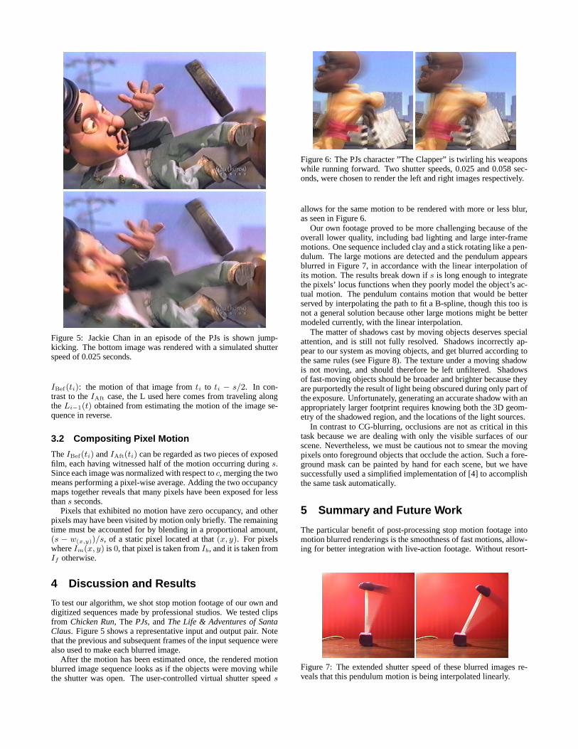
Figure 5: Jackie Chan in an episode of the PJs is shown jump-kicking. The bottom image was rendered with a simulated shutterspeed of 0.025 seconds.

IBef(ti): the motion of that image from ti to ti − s/2. In con-trast to the IAft case, the L used here comes from traveling alongthe Li−1(t) obtained from estimating the motion of the image se-quence in reverse.

3.2 Compositing Pixel Motion

The IBef(ti) and IAft(ti) can be regarded as two pieces of exposedfilm, each having witnessed half of the motion occurring during s.Since each image was normalized with respect to c, merging the twomeans performing a pixel-wise average. Adding the two occupancymaps together reveals that many pixels have been exposed for lessthan s seconds.

Pixels that exhibited no motion have zero occupancy, and otherpixels may have been visited by motion only briefly. The remainingtime must be accounted for by blending in a proportional amount,(s − w(x,y))/s, of a static pixel located at that (x, y). For pixelswhere Im(x, y) is 0, that pixel is taken from Ib, and it is taken fromIf otherwise.

4 Discussion and Results

To test our algorithm, we shot stop motion footage of our own anddigitized sequences made by professional studios. We tested clipsfrom Chicken Run, The PJs, and The Life & Adventures of SantaClaus. Figure 5 shows a representative input and output pair. Notethat the previous and subsequent frames of the input sequence werealso used to make each blurred image.

After the motion has been estimated once, the rendered motionblurred image sequence looks as if the objects were moving whilethe shutter was open. The user-controlled virtual shutter speed s

Figure 6: The PJs character ”The Clapper” is twirling his weaponswhile running forward. Two shutter speeds, 0.025 and 0.058 sec-onds, were chosen to render the left and right images respectively.

allows for the same motion to be rendered with more or less blur,as seen in Figure 6.

Our own footage proved to be more challenging because of theoverall lower quality, including bad lighting and large inter-framemotions. One sequence included clay and a stick rotating like a pen-dulum. The large motions are detected and the pendulum appearsblurred in Figure 7, in accordance with the linear interpolation ofits motion. The results break down if s is long enough to integratethe pixels’ locus functions when they poorly model the object’s ac-tual motion. The pendulum contains motion that would be betterserved by interpolating the path to fit a B-spline, though this too isnot a general solution because other large motions might be bettermodeled currently, with the linear interpolation.

The matter of shadows cast by moving objects deserves specialattention, and is still not fully resolved. Shadows incorrectly ap-pear to our system as moving objects, and get blurred according tothe same rules (see Figure 8). The texture under a moving shadowis not moving, and should therefore be left unfiltered. Shadowsof fast-moving objects should be broader and brighter because theyare purportedly the result of light being obscured during only part ofthe exposure. Unfortunately, generating an accurate shadow with anappropriately larger footprint requires knowing both the 3D geom-etry of the shadowed region, and the locations of the light sources.

In contrast to CG-blurring, occlusions are not as critical in thistask because we are dealing with only the visible surfaces of ourscene. Nevertheless, we must be cautious not to smear the movingpixels onto foreground objects that occlude the action. Such a fore-ground mask can be painted by hand for each scene, but we havesuccessfully used a simplified implementation of [4] to accomplishthe same task automatically.

5 Summary and Future Work

The particular benefit of post-processing stop motion footage intomotion blurred renderings is the smoothness of fast motions, allow-ing for better integration with live-action footage. Without resort-

Figure 7: The extended shutter speed of these blurred images re-veals that this pendulum motion is being interpolated linearly.

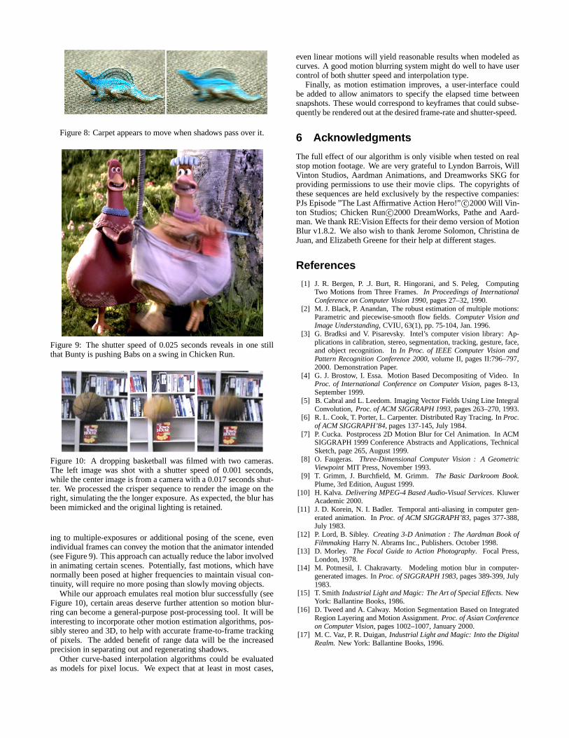
Figure 8: Carpet appears to move when shadows pass over it.

Figure 9: The shutter speed of 0.025 seconds reveals in one stillthat Bunty is pushing Babs on a swing in Chicken Run.

Figure 10: A dropping basketball was filmed with two cameras.The left image was shot with a shutter speed of 0.001 seconds,while the center image is from a camera with a 0.017 seconds shut-ter. We processed the crisper sequence to render the image on theright, simulating the the longer exposure. As expected, the blur hasbeen mimicked and the original lighting is retained.

ing to multiple-exposures or additional posing of the scene, evenindividual frames can convey the motion that the animator intended(see Figure 9). This approach can actually reduce the labor involvedin animating certain scenes. Potentially, fast motions, which havenormally been posed at higher frequencies to maintain visual con-tinuity, will require no more posing than slowly moving objects.

While our approach emulates real motion blur successfully (seeFigure 10), certain areas deserve further attention so motion blur-ring can become a general-purpose post-processing tool. It will beinteresting to incorporate other motion estimation algorithms, pos-sibly stereo and 3D, to help with accurate frame-to-frame trackingof pixels. The added benefit of range data will be the increasedprecision in separating out and regenerating shadows.

Other curve-based interpolation algorithms could be evaluatedas models for pixel locus. We expect that at least in most cases,

even linear motions will yield reasonable results when modeled ascurves. A good motion blurring system might do well to have usercontrol of both shutter speed and interpolation type.

Finally, as motion estimation improves, a user-interface couldbe added to allow animators to specify the elapsed time betweensnapshots. These would correspond to keyframes that could subse-quently be rendered out at the desired frame-rate and shutter-speed.

6 Acknowledgments

The full effect of our algorithm is only visible when tested on realstop motion footage. We are very grateful to Lyndon Barrois, WillVinton Studios, Aardman Animations, and Dreamworks SKG forproviding permissions to use their movie clips. The copyrights ofthese sequences are held exclusively by the respective companies:PJs Episode ”The Last Affirmative Action Hero!” c©2000 Will Vin-ton Studios; Chicken Run c©2000 DreamWorks, Pathe and Aard-man. We thank RE:Vision Effects for their demo version of MotionBlur v1.8.2. We also wish to thank Jerome Solomon, Christina deJuan, and Elizabeth Greene for their help at different stages.

References

[1] J. R. Bergen, P. .J. Burt, R. Hingorani, and S. Peleg, ComputingTwo Motions from Three Frames. In Proceedings of InternationalConference on Computer Vision 1990, pages 27–32, 1990.

[2] M. J. Black, P. Anandan, The robust estimation of multiple motions:Parametric and piecewise-smooth flow fields. Computer Vision andImage Understanding, CVIU, 63(1), pp. 75-104, Jan. 1996.

[3] G. Bradksi and V. Pisarevsky. Intel’s computer vision library: Ap-plications in calibration, stereo, segmentation, tracking, gesture, face,and object recognition. In In Proc. of IEEE Computer Vision andPattern Recognition Conference 2000, volume II, pages II:796–797,2000. Demonstration Paper.

[4] G. J. Brostow, I. Essa. Motion Based Decompositing of Video. InProc. of International Conference on Computer Vision, pages 8-13,September 1999.

[5] B. Cabral and L. Leedom. Imaging Vector Fields Using Line IntegralConvolution, Proc. of ACM SIGGRAPH 1993, pages 263–270, 1993.

[6] R. L. Cook, T. Porter, L. Carpenter. Distributed Ray Tracing. In Proc.of ACM SIGGRAPH’84, pages 137-145, July 1984.

[7] P. Cucka. Postprocess 2D Motion Blur for Cel Animation. In ACMSIGGRAPH 1999 Conference Abstracts and Applications, TechnicalSketch, page 265, August 1999.

[8] O. Faugeras. Three-Dimensional Computer Vision : A GeometricViewpoint MIT Press, November 1993.

[9] T. Grimm, J. Burchfield, M. Grimm. The Basic Darkroom Book.Plume, 3rd Edition, August 1999.

[10] H. Kalva. Delivering MPEG-4 Based Audio-Visual Services. KluwerAcademic 2000.

[11] J. D. Korein, N. I. Badler. Temporal anti-aliasing in computer gen-erated animation. In Proc. of ACM SIGGRAPH’83, pages 377-388,July 1983.

[12] P. Lord, B. Sibley. Creating 3-D Animation : The Aardman Book ofFilmmaking Harry N. Abrams Inc., Publishers. October 1998.

[13] D. Morley. The Focal Guide to Action Photography. Focal Press,London, 1978.

[14] M. Potmesil, I. Chakravarty. Modeling motion blur in computer-generated images. In Proc. of SIGGRAPH 1983, pages 389-399, July1983.

[15] T. Smith Industrial Light and Magic: The Art of Special Effects. NewYork: Ballantine Books, 1986.

[16] D. Tweed and A. Calway. Motion Segmentation Based on IntegratedRegion Layering and Motion Assignment. Proc. of Asian Conferenceon Computer Vision, pages 1002–1007, January 2000.

[17] M. C. Vaz, P. R. Duigan, Industrial Light and Magic: Into the DigitalRealm. New York: Ballantine Books, 1996.