IMA Mathematical Modeling in IndustryWorkshop 2005: Integrated Circuit Layout

Reconstruction

Ian Besse∗, Patrick Campbell†, Julianne Chung‡, Malena I. Espanol§,

Mark Iwen¶, Edward Keyes (Mentor)‖, Qingshuo Song∗∗

August 22, 2005

Abstract

We present a heuristic algorithm for the reconstruction of inte-grated circuit layout represented by polygons. The algorithm we pro-pose both reduces the number of vertices and recreates original shapesby reconstructing the polygons using only orthogonal and 45 degreelines.

1 Introduction

Integrated Circuits (IC) are designed using a polygon representation of thewiring and transistors layers known as ”layout”. Layout must conform tostrict design rules. Typically the design rules describe the minimum widthof any polygon, minimum spacing between adjacent polygons, directionality(normally only vertical, horizontal and sometimes 45 degree lines are allowed.

∗University of Iowa†Los Alamos National Laboratory‡Emory University§Tufts University¶University of Michigan‖Semicondutor Insights∗∗Wayne State University

1

Multiple wiring layers are common, with modern ICs having as many as tenwiring levels. Different wiring layers are connected through a contact or ”via”level. The via levels must also obey their own set of design rules on size andspacing.

The process of analyzing the design of an integrated circuit involves imag-ing the various layers and then using image processing to reconstruct thelayout of the different layers. Built-in biases, both in the manufacturing pro-cess and the analysis process prevent the reconstructed layout from being afaithful representation of the original layout. For example, sharp corners be-come rounded, line widths may either expand or contract and straight linesbecome roughened with many false vertices.

The original layout must be recreated from the raw polygon data. Thereare a number of potential errors that must be avoided in any reconstructionscheme including: creation of shorts between adjacent polygons, creationof a break or ”open” in an existing polygon or creation of self intersectingpolygons.

In this report, we present a heuristic algorithm to deal with this problemand evaluate the performance of our algorithm on a variety of test problems.The paper is organized as follows: Section 2 includes the basic problemand explains the energy function underlying the problem. Then, Section 3explains the various details of our algorithm, and some numerical results aredisplayed in Section 4.

2 The Basic Problem

Given a polygon P we would like to approximate it with another polygon Qhaving the following properties:

1. Q’s maximum deviation from P is small. In other words, we want Qto capture P’s general shape.

2. Q should include as much of the region bounded by P as possible. Pis ultimately a metal line connecting vias. Q will continue to intersectall the vias connected by P as long as Q contains P. Hence, we wouldlike Q to be a ’fattened’ version of P.

3. The fewer vertices Q contains the better.

2

4. We prefer that Q consists entirely of vertical, horizontal, 45 degree,and 135 degree lines since they are the only types of lines that shouldappear in standard IC layouts.

To determine what polygons better approximate P we utilize an energyfunction. The IC layout problem then reduces to optimizing the energy ofapproximating polygons. We next propose an energy function that addressesthe four preceding properties.

Given a polygon P = (x1, y1), (x2, y2), ...(xN , yN) and an approximatingpolygon Q = (x′1, y

′1), (x

′2, y

′2), ...(x

′M , y′M) we define the maximum deviation

of Q from P as follows:For any polygon R and point s let dist(s,R) = mindist(s, r)| r is on polygon R.

The maximum deviation of Q from P is defined as

dev(Q,P ) = maxdist(p,Q)| p is a point onP∪dist(q, P )|q is a point on Q.

In order to express that Q is better when it deviates less from P we includethe following term in our energy function:

α ∗ eβ∗(dev(Q,P )−ε).

We also want to bias towards having Q include all of P ’s interior pointsas per the second condition above. In order to help express this ’fattening’bias we define P − Q to be the set of points contained in P but not in Q.And, as one might expect, we let Area(P−Q) = the area of the region P−Qin the Euclidean plane. In order to express that Q is better when it includesmore of the region bounded by P we include the following term in our energyfunction:

γ ∗ eδ∗Area(P−Q).

To represent the desirability of horizontal, vertical, 45 degree, and 135degree lines we also include the energy function term

τ ∗M∑i=1

sin2(4∗sin−1(|yi−yi+1modM |/√

(xi − xi+1modM)2 + (yi − yi+1modM)2)).

Given P , the energy of our approximation Q is then given by

Energy(Q) = M + α ∗ eβ∗(dev(Q,P )−ε) + γ ∗ eδ∗Area(P−Q)

3

+τ ∗M∑i=1

sin2(4 ∗ sin−1(|yi − yi+1modM |√

(xi − xi+1modM)2 + (yi − yi+1modM)2)).

We are now ready to state our problem: Given a polygon P we wish tofind an approximating polygon Q such that Energy(Q) is minimized.

Our solution proceeds by greedily choosing the portion of P ’s boundarywhose approximation by a line yields the greatest decrease in energy. Wethen ’repair’ the boundary and repeat the process on the next best portionof P ’s boundary. As it will be discussed in the next section, casting theproblem as an optimization problem allows the use of fast efficient heuristicapproaches (such as greedy pursuit).

3 The GROS Algorithm

A typical layout data set contains millions of polygons. Any simplificationalgorithm must be computationally inexpensive. Even an approximate solu-tion of the above energy equation is impractical. Certainly, if computationalefficiency was not a factor, one could generate an optimal or very near optimalalgorithm for attaining the minimal energy. However, since this algorithmneeds to be practical in a business context, we must choose to forego somemathematical exactness and use a more heuristic solution.

To address the issue of fidelity, we first designate a fidelity factor, a max-imum allowable deviation that a simplified edge can have from an originaledge. This ε depends heuristically upon the scale of the features in the poly-gon. Deviations of a polygon edge of less than ε/2 are considered to beinconsequential.

To satisfy the angular energy in the energy function we adopt the rulethat we always repair (whenever repair is possible) with segments that areonly horizontal, vertical or 45 degree diagonal.

To reduce the vertex energy term we adopt a rule which replaces longchains of vertices by a single two vertex segment provided all the replacedvertices are within our fidelity metric (ε/2) of the proposed segment.

Additionally, intuition dictates that a greedy approach to decimation beemployed. Thus, before the repair portion of the algorithm begins, a searchfor the longest sequence of vertices satisfying our tolerance conditions is con-ducted and the identified sequence is the sequence which is repaired first.Our algorithm then proceeds in a clockwise direction from that point on-

4

ward. Ultimately, an algorithm which leaps from the longest to the nextlongest such sequence would be preferable as the number of vertices wouldthen follow the path of greatest descent. With these considerations in mind,we proceed with a detailed explanation of the GROS algorithm.

3.1 Finding the Safety Factor

Not only is it important to ensure faithful reconstruction of the originalpolygon edges but also we must be careful of its neighboring polygons. Joinsbetween the original polygon and its neighbors must be avoided. The amountby which a polygon edge may be moved without joining to another polygonis a crucial part of any reconstruction algorithm.

Given a particular polygon, the process of finding a proper safety factorS begins by first finding the neighbor polygons. This is done by finding theminimum and maximum x and y values of the polygon and creating boundingboxes around each polygon. Then we pad them to find its neighbors. Thencompute intersection between each box and its surrounding boxes and onlybetween them find polygon distance.

3.1.1 Minimum distance between non-convex polygons

In this subsection, we assume self-intersection does not happen for simplicity.To proceed, we define the minimum distance between two disjoint polygonsas

dist(P, Q) := minp∈P,q∈Q

dist(p, q) (1)

We introduce a naive approach for calculating S, so that the polygons donot intersect to each other within the S change.

1. Given a maximum S, and a finite set of polygons Ω,

2. For each polygon P , find

ε1 = minQ∈Ω

dist(P,Q), (2)

3. Set the S for polygon P as §p = min§1, §.

Therefore, the safety factor calculation comes up with calculation of dist(P, Q)for arbitrary disjoint polygons P and Q. The minimum distance between two

5

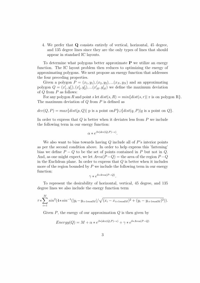
polygons P and Q is determined by anti-podal pair between the polygons.As there are three cases for anti-podal pairs between polygons, three casesfor the minimum distance can occur:

1. The vertex-vertex case, see Figure 1 (a),

2. The vertex-edge case, see Figure 1 (b),

3. The edge-edge case, see Figure 1 (c).

In other words, the points determining the minimum distance are notnecessarily vertices.

(a) vertex–vertex case (b) vertex–edge case (c) edge–edge case

Figure 1: Three cases for anti-podal pairs between polygons

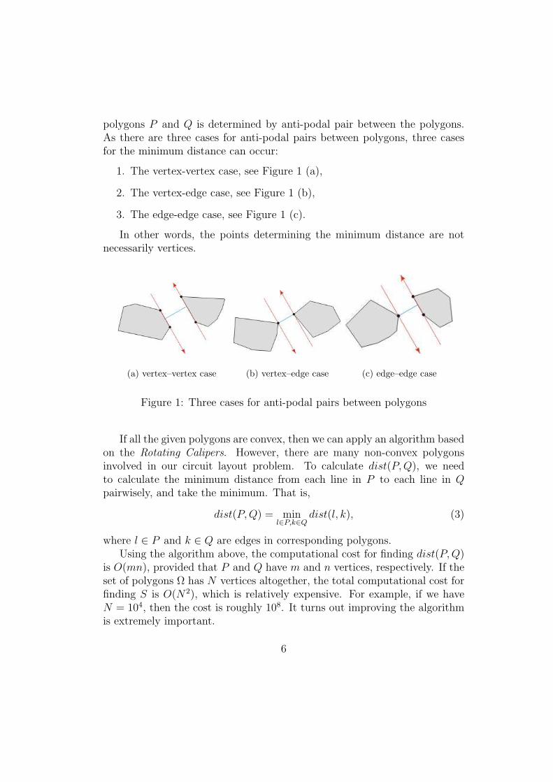
If all the given polygons are convex, then we can apply an algorithm basedon the Rotating Calipers. However, there are many non-convex polygonsinvolved in our circuit layout problem. To calculate dist(P, Q), we needto calculate the minimum distance from each line in P to each line in Qpairwisely, and take the minimum. That is,

dist(P, Q) = minl∈P,k∈Q

dist(l, k), (3)

where l ∈ P and k ∈ Q are edges in corresponding polygons.Using the algorithm above, the computational cost for finding dist(P,Q)

is O(mn), provided that P and Q have m and n vertices, respectively. If theset of polygons Ω has N vertices altogether, the total computational cost forfinding S is O(N2), which is relatively expensive. For example, if we haveN = 104, then the cost is roughly 108. It turns out improving the algorithmis extremely important.

6

3.1.2 Neighborhood approach

To reduce the computational cost, we want to replace (2) by

§1 = minQ∈N(P )

dist(P, Q) (4)

where N(P ) is the neighborhood of P . The basic idea is that, we onlycalculate the distance to those polygons in the neighborhood of P .

Before precisely presenting the definition of N(P ), we need to introduceseveral notations. Let px and py be x− and y− coordinates of vertex p ∈ P .Also let

xm(P ) = minp∈P

px, ym(P ) = minp∈P

py,

andxM(P ) = max

p∈Ppx, yM(P ) = max

p∈Ppy.

Construct rectangle P § with diagonal (xm(P )− §, ym(P )− §) and (xM(P ) +ε, yM(P ) − §). In such a way, P § gives a rectangle which is enlarged by §from each side of convex hull of P .

The most important property of this simplification of polygons is that acomplex object is represented by a limited number of bytes. Although a lotof information is lost, neighborhood rectangles of spatial objects preserve themost essential geometric properties of the object, that is, the location of theobject and the extension of the object in each axis. For realistic profiles ofdata and operations, the gain in performance is quite considerable.

Now we define N(P ) as following:

N(P ) = Q ∈ Ω : P § ∩Q§ 6= Φ. (5)

To implement (4), we need to use following fact: Two rectangles P § and Q§

intersect to each other if and only if it satisfies

xm(P §) < xM(Q§) & xm(Q§) < xM(P §) (6)

ym(P §) < yM(Q§) & ym(Q§) < yM(P §). (7)

In the last subsection, we calculate dist(P, Q) by finding distance fromline to line pairwisely. However, it is very often that some lines in P are farapart from Q. To save consuming cost for dist(P,Q), we replace (3) with

dist(P,Q) = minl∈N(Q),k∈N(P )

dist(l, k) (8)

where l and k are edges in P and Q respectively. We can use (6) and (7) toverify if l ∈ N(Q) for all l ∈ P.

7

3.1.3 Tolerance for each vertex in direction

In Figure 2 (a), the safe move distances to the right upwards differ consider-ably. It is therefore beneficial to allow safety factors for each vertex in eachdirection. We therefore need 4 directions to consider for each vertex: up,down, left, right.

p

(a)

ε

p

q1

q2

(b)

Figure 2: various Safety Factors for each direction each vertex

For illustration, we explain the case in Figure 2 (b). Suppose we want toadjust vertex p upwards.

1. construct upward neighborhood rectangle p§ for p containing adjacentedges.

2. calculate §1 similar to (4).

§1 = mini=1,2,l∈N(p)

dist(l, ¯qpi) (9)

In the above, l is line segment, such that,

l ∈ N(p) := l ∈ Ω : l ∩ p§ 6= Φ.

The advantage of this method is that we can avoid self-intersection in ourwork.

8

3.2 Finding the Optimal Starting Sequence

Before we run the repair algorithm, we run a routine to find the longest se-quence of vertices which satisfies the following two conditions: 1) the pairwisedistance between the vertices must be less than a fidelity tolerance ε in eitherthe x or y direction, and 2) the sequence of Euclidian distances between thefirst vertex and each subsequent vertex, must be monotonically increasing.That is, we want the longest sequence, < v1, v2, . . . , vn > such that

‖vi − vj‖∞ < ε

for all i, j ≤ n, and‖vi − v1‖2 ≤ ‖vi+1 − v1‖2

for i = 1, . . . , n.We choose the vertex at the beginning of the sequence as the starting

point of our repair routine because the sequence is presumably relativelystraight, and contains no switchbacks.

Figure 3: A sequence satisfying our criteria

3.3 Repair Algorithm

Once the longest sequence of vertices satisfying our vertical and horizontaltolerance conditions has been identified, the repair of the polygon may com-mence. Ultimately, the algorithm for identifying the longest viable sequence

9

of vertices will search in all four directions, but ours does not currently sup-port this feature. Thus, the repair algorithm as it currently stands uses onlythe information about the location of the longest viable sequence to deter-mine a starting vertex and conducts its own search for a viable sequence fromthere. In order to understand the repair algorithm, the diagram in Figure4 may be helpful. The diagram shows an initial vertex in the center and

Figure 4: Bounding bands enclosing a sequence of vertices.

the sequence of consecutive vertices extending from it. As one progressesfrom one vertex to the next, one or more of the four bounding bands may beexited. Once this occurs, the algorithm raises a flag to indicate the directionof the violation. As soon as a flag has been raised at least once for each ofthe bounding bands, the we have reached a stop-and-repair condition.

If at the first step, the vertex adjacent to the initial vertex immediatelyexits all four of the bounding bands, the algorithm then checks to see if theoffending vertex has exited horizontal and vertical bounding bands whichare twice as wide as the original. If it has, then we make no repair to thesegment and proceed using the offending vertex as the new initial vertex.

10

If the offending vertex is within twice our tolerance in either the verticalor horizontal directions the algorithm generates the appropriate horizonalor vertical line midway between the two vertices and generates two newvertices that are the projections of each vertex onto that line. The algorithmresumes its search for viable sequences using the offending vertex as a newinitial vertex.

If the offending vertex is not adjacent to the initial vertex, then theprevious, non-offending vertex is then considered the terminal vertex in whatis a viable sequence. The algorithm then proceeds to conduct a implicationof that sequence based on a number of conditions. If the last bounding bandto be flagged is either of the diagonals, then the simplification is merely todecimate all vertices whose indices are strictly between those of the initial andterminal vertices. In the horizontal and vertical directions, the simplificationfollows what we call the “always fatten” rule. Note that in both the horizontaland vertical cases, we may replace the sequence with two edges, one verticaland one horizontal. Such a replacement is not unique, however. We have twochoices for generating the middle replacement vertex as shown in the Figure5

Figure 5: The figure on the left results in greater area for our simplifiedpolygon.

The algorithm generates the vertex which results in the capture of agreater portion of the interior of the polygon. This choice is an effort toreduce the likelihood of narrowing a polygon to zero width in some spotsand also to reduce the likelihood of self-intersection.

During this process of simplifying sequences, redundancies may have beencreated and “hanging chads,” vertices which stick out on a line segment fromthe polygon, may be left behind. The final process in the repair algorithm

11

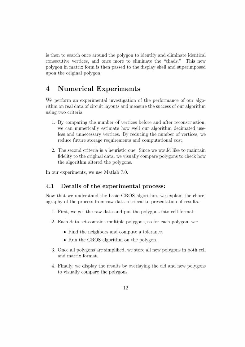
is then to search once around the polygon to identify and eliminate identicalconsecutive vertices, and once more to eliminate the “chads.” This newpolygon in matrix form is then passed to the display shell and superimposedupon the original polygon.

4 Numerical Experiments

We perform an experimental investigation of the performance of our algo-rithm on real data of circuit layouts and measure the success of our algorithmusing two criteria.

1. By comparing the number of vertices before and after reconstruction,we can numerically estimate how well our algorithm decimated use-less and unnecessary vertices. By reducing the number of vertices, wereduce future storage requirements and computational cost.

2. The second criteria is a heuristic one. Since we would like to maintainfidelity to the original data, we visually compare polygons to check howthe algorithm altered the polygons.

In our experiments, we use Matlab 7.0.

4.1 Details of the experimental process:

Now that we understand the basic GROS algorithm, we explain the chore-ography of the process from raw data retrieval to presentation of results.

1. First, we get the raw data and put the polygons into cell format.

2. Each data set contains multiple polygons, so for each polygon, we:

• Find the neighbors and compute a tolerance.

• Run the GROS algorithm on the polygon.

3. Once all polygons are simplified, we store all new polygons in both celland matrix format.

4. Finally, we display the results by overlaying the old and new polygonsto visually compare the polygons.

12

4.2 Some Good results

Running the GROS algorithm on a plethora of real test data polygons, wefound that, for the most part, our algorithm did an excellent job at elimi-nating unnecessary vertices and squaring off jagged edges and corners. Weencountered many successful reconstructions, but in this section, we onlylook at two such examples. In Figure 6, the yellow polygons with blue ver-tices represent the original polygon data. Especially evident in the 45 degreepolygons, we see an excess of vertices. To compare the original with the newpolygons we overlay the original polygons with the red simplified polygons,which have red dots as the vertices.

The success of our algorithm is evident in both cases, orthogonal and 45degree angles, but we see that in Figure 6, the polygon containing the 45degree angle had a 61 % reduction in vertices on that polygon alone. We willsee that in larger cases that contain 45 degree angles, the reduction can beextremely significant.

4.3 Analysis/Comparison

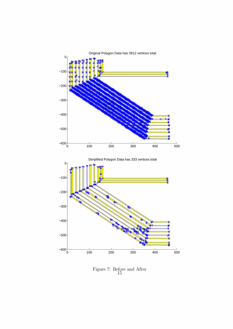
• In the previous subsection, we looked at smaller cases of polygons togage how well our algorithm performed. However, many of the actualdata polygon sets contain hundreds to thousands of polygons and thou-sands to millions of vertices. To illustrate the power of our algorithm,we compare the before and after images of one of the larger sets of poly-gons. Figure 7 shows the original polygons and the simplified polygons.The blue stars represent the polygon vertices. There are 3912 verticesfor the original data and 333 vertices for the simplified data, which isa significant decrease in storage. In addition, we kept the features ofthe original polygons.

• Another factor that can affect our results is the tolerance. In thissection we consider the tradeoff between tolerance size and percentagedecrease in the number of vertices. We run our algorithm on exampledata, and we compare the results with respect to the tolerance. Weonly measure with respect to the first criteria, comparing the originalnumber of vertices and the new number of vertices. Our results aredisplayed in Figure 8 and we can see the incremental change in behavioras the tolerance increases.

13

Figure 6: Good reconstructions

14

0 100 200 300 400 500−600

−500

−400

−300

−200

−100

0Original Polygon Data has 3912 vertices total

0 100 200 300 400 500−600

−500

−400

−300

−200

−100

0Simplified Polygon Data has 333 vertices total

Figure 7: Before and After15

Though we see in Figure 8 that a higher tolerance can result in lessvertices, we must be cautious of tolerances which are too large. Wehave observed that the fidelity decreases as the tolerance increases, soit is a tradeoff between both.

0 2 4 6 820

30

40

50

60

70

80

Tolerance

Per

cent

age

decr

ease

of v

ertic

es

Figure 8: Tolerance vs. Percentage decrease in vertices

4.4 Some problems we encountered

Though our algorithm repaired many polygons as expected, there were someproblems that we encountered. With our current approach, there exists thepotential of creating self-intersections. For example, with a tolerance toolarge on a 45 degree polygon, we may get polygons like that shown in Figure9.

16

Figure 9: A Self intersection on a 45 degree polygon

17

Also, depending on the starting line segment, it is possible to create selfintersection ”holes” like that shown in Figure 10.

5 Conclusions

We presented an heuristic algorithm to reconstruct an integrated circuit lay-out. We have shown the details of the implementation: the computation ofa fidelity factor, the greedy approach to vertex decimation and the rules as-sociated with the repair of an edge. The results generated by our algorithm,both numerical and graphical, provide evidence that our approach is quitesuccessful.

Aside from relatively few instances in which our algorithm producesanomalous results, the algorithm seems to converge to a solution which sig-nificantly reduces the energy of the polygon sets. In many cases, the numberof vertices, the primary factor in determining image file size, is significantlyreduced from the original number. Visual inspection of the simplified poly-gons indicates that in most cases a high degree of fidelity has been maintainedand once-ragged edges have been rendered quite crisp.

Future work may resolve the problems with self-intersection and the emer-gence of anomalous holes in the polygons. In addition, a more effectivemethod of determining the fidelity factor could not only speed up the com-putations, but if a vertex-specific variable tolerance could be determined, itwould likely result in a great increase in fidelity.

6 Acknowledgements

The authors would like to acknowledge the support from the Institute ofMathematics and its Applications. We would also like to thank Steve Begg,Senior Software Developer, Martin Strauss, University of Michigan, andSuresh Venkatasubramanian, AT&T Labratory.

18

Figure 10: Self intersection hole

19