1111111 111111111111111 Ill Ill Ill Report No. DTRSSG-96-C-0010 Task 1 and 2 Final Report

PB99-138356

In-Line Inspection Technologies for Mechanical Damage and sec in Pipelines - Final Report on Tasks

1 and 2

prepared by T. A. Bubenik, J. B. Nestleroth, and R. J. Davis, Battelle

A. Crouch, Southwest Research Institute S. Udpa and M. A. K. Afzal, Iowa State University

for

U. S. Department of Transportation, Office of Pipeline Safety 400 Seventh Street, SW Washington, DC 20590

Lloyd Ulrich, Contracting Officer's Technical Representative December 1998

Contract No. DTRSSG-96-C-0010

This document is available to the U.S. Public through the

National Technical Information Center

REPRODUCED BY: N11S. U.S. Department of Commerce-·-­

National Technical lnfonnation Service Springfield, Virginia 22161

50272-101

REPORT DOCUMENTATION 11. REPORT NO. PAGE DTRS56-96-C-0010

2.

4. Title and Subtitle

In-Line Inspection Technologies for Mechanical Damage and SCC in Pipelines -Final Report on Tasks 1 and 2

7. Authors

T. A. Bubenik, J. B. Nestleroth, R. J.Davis, A. Crouch, S. Udpa, and M.A. K. Afzal

9. Performing Organization Name and Address

Battelle Southwest Research Institute 505 King Avenue 6220 Culebra Road Columbus, Ohio 43201-2693 San Antonio, Texas 78228-0510

12. Sponsoring Organization Name and Address

U.S. Department of Transportation Office of Pipeline Safety 400 Seventh Street SW Washington, DC 20590

15. Supplementary Notes

16. Abstract (Limit 200 Words)

I Reproduced from best available copy.

Iowa State University Ames, Iowa 50011

1111111 111111111111111 Ill Ill Ill PB99-138356

5. Report Date

December 1998

6.

8. Performing Organization Rept. No.

10. Project/Task/Work Unit No.

G002993-17

11. Contr. (C) or Grant (G) No.

(C) DTRS56-96-C-0010

(G)

13. Type of Report & Period Covered

14.

Final June 1996-September 1999

This report is a summary of work conducted under a research and development contract entitled "In-Line Inspection Technologies for Mechanical Damage and SCC (Stress-Corrosion Cracking) in Pipelines." This project evaluated and developed in-line inspection technologies for detecting mechanical damage and cracking in natural gas transmission and hazardous liquid pipelines. The work consists of three major tasks. Task 1 covers inspection methods for mechanical damage. Task 2 covers methods of detecting stress-corrosion cracks. Task 3 covers verification testing. This report is a summary of the work completed in the first two tasks.

Task 1 examined magnetic flux leakage (MFL) for detecting mechanical damage. It evaluated existing signal generation and analysis methods to establish a baseline from which today's tools can be evaluated and tomorrow's advances measured, and it developed improvements to signal analysis methods and verified them through pull rig testing. Finally, it built an experience base and defect sets to generalize the results from individual tools and analysis methods to the full range of practical applications. Task 2 evaluated two inspection technologies for detecting cracks. Three subtasks were conducted to evaluate velocity-induced remote-field techniques, remote-field eddy-current techniques, and external techniques for sizing stress­corrosion cracks.

17. Document Analysis a. Descriptors

b. Identifiers/Open-Ended Terms

Pipe, pipelines, magnetic flux leakage, inspection, in-line inspection, smart pig, mechanical damage, SCC, stress-corrosion cracking, natural gas, hazardous liquid

c. COSATI Field/Group

18. Availability Statement

Availability Unlimited

(See ANSl-239.18)

19. Security Class (This Report)

Unclassified

20. Security Class (This Page)

Unclassified

21. No. of Pages

22. Price

OPTIONAL FORM 272 (4-77) (Formerly NTIS-35) Department of Commerce

NOTICE

This document is disseminated under the sponsorship of the Department of Transportation in the interest of information exchange. The United States Government

assumes no liability of or the contents and use thereof.

This report is a work prepared for the United States Government by Battelle. In no event shall either the United States Government or Battelle have any responsibility or liability

for any conseq·uences of any use, misuse, inability to use, or reliance on the information contained herein, nor does either warrant or otherwise represent in any way the

accuracy, adequacy, efficacy, or applicability of the contents hereof.

PROTECTED UNDER INTERNATIONAL COPYRIGHT ALL RIGHTS RESERVED. 1NATIONAL TECHNICAL INFORMATION SERVICE U.S. DEPARTMENT OF COMMERCE

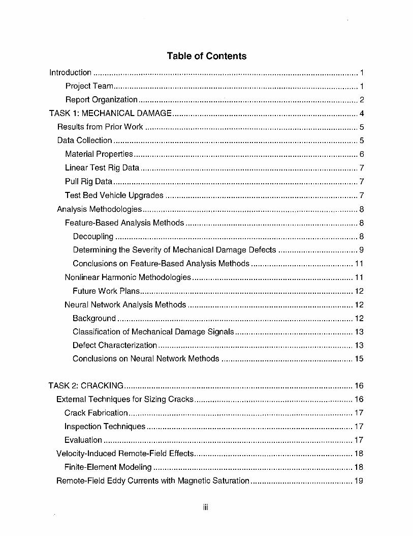
Table of Contents

Introduction ..................................................................................................................... 1

Project Team ............................................................................................................ 1

Report Organization ................................................................................................. 2

TASK 1: MECHANICAL DAMAGE .................................................................................. 4

Results from Prior Work .............................................................................................. 5

Data Collection ............................................................................................................ 5

Material Properties ................................................................................................... 6

Linear Test Rig Data ................................................................................................ 7

Pull Rig Data ............................................................................................................ 7

Test Bed Vehicle Upgrades ..................................................................................... 7

Analysis Methodologies ............................................................................................... 8

Feature-Based Analysis Methods ............................................................................ 8

Decoupling ........................................................................................................... 8

Determining the Severity of Mechanical Damage Defects ................................... 9

Conclusions on Feature-Based Analysis Methods ............................................. 11

Nonlinear Harmonic Methodologies ....................................................................... 11

Future Work Plans .............................................................................................. 12

Neural Network Analysis Methods ......................................................................... 12

Background ........................................................................................................ 12

Classification of Mechanical Damage Signals .................................................... 13

Defect Characterization ...................................................................................... 13

Conclusions on Neural Network Methods .......................................................... 15

TASK 2: CRACKING ..................................................................................................... 16

External Techniques for Sizing Cracks ...................................................................... 16

Crack Fabrication ................................................................................................... 17

Inspection Techniques ........................................................................................... 17

Evaluation .............................................................................................................. 17

Velocity-Induced Remote-Field Effects ...................................................................... 18

Finite-Element Modeling ........................................................................................ 18

Remote-Field Eddy Currents with Magnetic Saturation ............................................. 19

iii

Experiments ........................................................................................................... 20

Conclusions on Magnetic Saturation ...................................................................... 20

Conclusions .................................................................................................................. 21

Task 3 Plans .............................................................................................................. 22

iv

INTRODUCTION

This report is a summary of work conducted for the U. S. Department of Transportation Office of Pipeline Safety under a research and development contract entitled "In-Line Inspection Technologies for Mechanical Damage and SCC (Stress-Corrosion Cracking) in Pipelines." This project is evaluating and developing in-line inspection technologies for detecting mechanical damage and cracking in natural gas transmission and hazardous liquid pipelines. The work consists of three major tasks. Task 1 covers inspection methods for mechanical damage. Task 2 covers methods of detecting stress­corrosion cracks. Task 3 covers verification testing.

~Link to Task 1 Workplan ~Link to Task 2 Workplan ~Link to Task 3 Plans

The purpose of this report is to summarize the work completed and conclusions drawn from Tasks 1 and 2 of this program. The intended audience is government representatives, pipeline companies, and inspection vendors. The actual data and technical analyses are documented separately.

The ultimate benefit of the project is expected to be more efficient and cost-effective operation, maintenance, and safety of transmission pipelines. Pipeline companies will benefit by having access to inspection technologies for detecting critical mechanical damage and cracks, and inspection vendors will benefit by understanding where improvements to their systems are beneficial and needed and how to make those improvements. These benefits, and others, will support the Office of Pipeline Safety's long-range objective of ensuring the safety and reliability of the pipeline infrastructure.

Project Team

The work conducted under this program is a joint effort of three organizations. Battelle acts as the prime contractor and is responsible for ensuring that the overall goals of the program are met. Southwest Research Institute is heavily involved in work to determine the effects of stresses and strains on the magnetic properties of pipeline steels, work on nonlinear harmonic sensors, and work on stress-corrosion cracking. Iowa State University is responsible for the work on neural networks, other advanced analysis techniques, and stress-corrosion cracking. Battelle is responsible for the remaining technical tasks.

1

Report Organization

This report is written in a Web format. The body of the report (this document) is an Executive Summary with links to additional details. This format will let readers quickly access more detailed information of interest to them. The Table of Contents lists the main sections of the report. Within each section, there are links to background and more detailed information on various topics. This report is being distributed as a printed copy of the body of the report along with a compact disk containing the entire report and all of its links. The links and glossary can be printed out for easy reference.

Links are identified with a document icon (r2il'), a figure icon (ifiJ), a video icon (II), an underline, or a button. Typically, document links open in place of the current document (which can be accessed again by pressing the back key); figure and video links open in a separate window; and underlined links (without an icon) redirect the user to another location on the same page or to an external Internet link. The text on a button will identify its use; buttons can redirect the user, open windows, allow the reader to download a video clip, or launch an external program. In addition, there is an on-line glossary. Words listed in italics are included in the glossary.

This report has three main sections: (1) Task 1 - Mechanical Damage, (2) Task 2 -Cracking, and (3) Conclusions. The first section, "Task 1 - Mechanical Damage,"

contains the following sections:

"Results from Prior Work" describes the basic components of inspection signals from mechanical damage, identifies key signal parameters and features, and summarizes conclusions from prior work.

"Data Collection" describes the defect fabrication process and the test equipment used to record inspection signals, summarizes the data taken, and summarizes the conclusions drawn about the basic magnetic properties of common pipeline steels.

"Analysis Methodologies" describes feature-based analysis methods, neural network analysis methods, and the use of nonlinear harmonic systems to detect and characterize mechanical damage.

The second section, "Task 2 - Cracking," contains the following sections:

"External Techniques for Sizing Cracks" summarizes work done here on a method of sizing tight cracks from the outer pipeline surface.

"Velocity Induced Eddy Currents" summarizes work to date on inspections via eddy currents that are generated near magnetic flux leakage (MFL) magnetizers.

2

"Remote Field Eddy Currents" summarizes work on defining the effect of magnetic saturation on remote field inspection techniques.

"Conclusions" summarizes the important findings from this program.

3

TASK 1: MECHANICAL DAMAGE

Magnetic flux leakage, or MFL, is the most commonly used in-line inspection method for the detection of corrosion in pipelines. rsubenik

921 Extending this technology for mechanical damage would simplify deployment and have many practical and economic benefits. MFL inspection tools locate pipeline defects by applying a magnetic field in the pipe wall and sensing a local change in this applied field with sensors near the pipe wall. These changes depend on the type of defect (metal loss or changes in material or magnetic properties).

12:Background material on MFL

MFL has been shown to be capable of detecting some mechanical damage. (Davis9S) (Davis97l

Part of the signal generated at mechanical damage is due to geometric changes - for example, a reduction in wall thickness due to metal loss causes an increase in measured flux and sensor/pipe separation (liftoff). Other parts of the signal are due primarily to changes in magnetic properties that result from stresses, strains, or damage to the microstructure of the steel.

~Background material on magnetic properties 12:Description of typical mechanical-damage features ~Background material on material property changes with stress and strain

Mechanical damage is the single largest cause of failures on gas-transmission pipelines today and a leading cause of failures on liquid transmission lines. Mechanical-damage defects typically show a number of features, such as denting, metal movement, and cold working. The most significant of these features from the perspective of defect severity are the size and extent of the cold worked region. From an inspection perspective, cold work, removed metal, denting, and residual stresses and strains are important. Cold work and residual stresses and strains change the magnetic properties of the steel, confounding inspection results. (AlhertonBSa. AlhertonBSb) Denting changes the orientation of the pipe wall with respect to the (typically) fixed orientation of sensors on an inspection tool. And removed metal produces a signal of its own, adding further complexity.

Inspection-tool variables, such as the strength of the applied magnetic field, impact the ability to detect and characterize defects. The applied magnetic field is a pivotal variable for detection of mechanical damage. The high magnetic fields used in many existing MFL inspection tools for detecting metal-loss defects such as corrosion cause a reduction in sensitivity to gouges.

Inspection-run variables, such as tool velocity and line pressure, also impact the results. Velocity reduces the strength of MFL signals. Pressure affects the stresses in the pipe wall (and adds stresses around dents and gouges), which in turn change the magnetic

4

properties of the pipe steel. Each of these effects changes the accuracy and reliability of MFL inspections.

Results from Prior Work

MFL signals for metal loss, dents, cold work, residual stresses, and plastic strains are fundamentally different. These differences create the potential to identify, decouple, and analyze different signal components as a means of assessing the severity of mechanical damage defects.

fz'Comparison off MFL signals for metal loss, dents, and cold work

MFL inspection tools that are designed to detect metal-loss corrosion are not optimized for detecting mechanical damage. These tools use high magnetic fields to suppress noise sources due to stresses and microstructural changes, such as cold work, which diminish sizing accuracy for corrosion. However, a mechanical-damage tool needs to detect changes in microstructure and stress. The results of previous studies show that the optimum field level for detecting cold work in mechanical damage is much lower and high field levels can mask or erase important components of the signal. Unfortunately, the noise sources that are avoided by high magnetizing fields become a part of the signal at low magnetization levels, making detection and characterization more difficult.

Basic effects of various parameters on MFL signals were measured in an earlier project. [Davis9Bl The prior results showed:

• Cold working typically increases the average magnetic permeability in the defect area, causing a decrease in the magnetic flux at the sensor

• The optimum magnetization point for detecting cold working (along with residual stresses and strains) is near the knee of the magnetization (8-H) curve. Conversely, the optimum magnetization point for corrosion detection is well above the knee into saturation.

Data Collection

A variety of different types of data have been taken in this program. In the first two subtasks, magnetic and mechanical properties of different pipe steels were measured. These measurements were made to ensure that later findings would be applicable to a wide variety of steels. Material property data were taken from 36 pipes that had been removed from service and from new pipe material.

Fabricated mechanical-damage defects were installed in flat plates, pipe sections, and full pipe pieces. In addition, a limited number of defects were collected from the field.

5

MFL measurements were made on these samples in the Gas Research Institute Pipeline Simulation Facility (PSF)n linear test rig and pull rig. In the future, similar data will be taken in the PSF flow loop.

G RI home page L6linear test rig [Nestleroth95l

f2i!pu II rig [Bubenik95al

Material Properties

Magnetic, mechanical, metallurgical, and chemical property data have been taken in this program. The magnetic properties of pipeline steels are variable and a function of fabrication process, alloying agents, and microstructure. Stress and strain play major roles in defining a steel's magnetic properties. Since stress and strain are important parts of mechanical damage, understanding their effects was a key part of this project.

Early in this program, magnetic and mechanical properties of different pipe steels were measured. rNeSt1er

0th981 Measurements were made on a subset of the samples under tensile and compressive loading. Additional measurements were made around a full pipe-circumference to ensure the findings would be apply to full pipe sections.

Ll6Description of basic material property testing BDescription of material property stress tests Ll6Description of full pipe tests f2i!Table of measured material property variations Ll6Typical database entry

This evaluation reached two main conclusions. First, there is no clear correlation between magnetic properties and commonly measured mechanical properties. So, the change in magnetic properties due to mechanical damage must be outside the range of typical magnetic properties in order for the damage to be detected. Alternatively, when assessment of mechanical damage defect signals requires data on actual magnetic properties, they must be measured because they cannot be estimated easily from the more commonly known mechanical properties.

The second conclusion is that the changes in magnetic properties due to compressive stresses are large enough to fall outside the typical scatter band of magnetic properties. So, detecting compressive stresses and strains may be possible without measuring the magnetic properties of a pipeline steel. The same cannot be said of tensile stresses. Tension causes more subtle property changes. So, detecting tensile stresses and strains would require measurements of magnetic properties in order to determine whether changes had occurred.

Based on the measurements made in this program, a database on the magnetic properties of steel, along with previously measured mechanical properties and chemical compositions, was compiled. rNeSt1ero

th981 Metallurgical data includes information on grain

6

size, grain distortion, inclusion size, density, and distribution. The database can be used as a basis for further developing MFL techniques and other inspection technologies to nondestructively determine a pipe's mechanical and magnetic properties.

Linear Test Rig Data

Linear test rig measurements were made at velocities under about 3 miles per hour, which is low enough that velocity is expected to have negligible effects. Typically, data were taken at 10 Oersted intervals, ranging from as low as 10 Oersted to as high as 150 Oersted. In addition, remanent measurements were taken using no applied field.

Three types of defects were investigated in the linear test rig: defects made under pressure, natural dent defects in pipe removed from service, and simple mechanical damage defects made in flat plates. The defects consisted of plain dents, cold worked regions, dents with cold worked regions, and cold worked regions with removed metal. The linear test rig defects were made in two pipe steels: the flow loop material and a generic X52 material. The materials used were the same as those used for the pull rig defects, discussed below.

li!Additional details on linear test rig experiments and defect sets i:rul"ypical L TR data

Pull Rig Data

Two types of defects were used in the pull rig. The pull rig defect sets included 38 defects made on pressurized pipe samples with a machine designed to make controlled dents and gouges roor9si and 32 defects made by hitting pressurized flow loop pipe with a backhoe. The pull rig defects included dent depths up to 6 percent of the pipe diameter. Gouge depths ranged from nearly zero to 25 percent of the wall thickness, and gouge lengths ranged from nearly zero to 6 inches. The defects were installed in two pipe samples, an X42 steel and an X60 steel, which were removed from service and donated to the program.

~Additional details on pull rig defects i:rul"ypical pull rig data

Test Bed Vehicle Upgrades

The linear test rig experiments showed that multiple magnetization levels provide additional information for detection and characterization of mechanical damage defects. However, the flux leakage levels needed are smaller for these defects than for metal loss. These results indicated that changes were required in the accuracy with which

7

data were taken with the MFL test bed vehicle. rNeSt1eroth961 To meet the data collection

needs, the magnetizer and sensors were modified and the electronics module was replaced. Other components, such as the battery system and the sensor wiring collar, were not changed. Mechanical components such as tow links, cups, and pressure vessels, were used as originally designed.

wsDescription of the MFL test bed vehicle fzAdditional details on the test bed vehicle modifications

Analysis Methodologies

Feature-Based Analysis Methods

Feature-based analysis methods make use of discrete signal parameters, such as peak amplitude or peak-to-peak amplitude. Peak amplitude is the maximum recorded value in an inspection signal, and peak-to-peak amplitude is the difference between the maximum and minimum recorded values in an inspection signal.

Feature-based analysis methods are commonly used by inspection vendors today. These methods typically preprocess data to determine the input to various algorithms that are used, for example, to determine the shape of a corrosion defect. Some feature­based analysis methods make adjustments to the overall defect signal, but these adjustments are a function of discrete signal features.

To improve the ability to reliably detect, classify, and size mechanical damage defects, Battelle developed a multiple magnetization approach. roavis

991 The approach requires two magnetizing levels: a high level for detecting geometric deformation and a low level for detecting both magnetic and geometric deformation. Classifying and determining the severity of the damage requires additional signal processing. A process called decoupling is used to extract unique signals due to geometric and magnetic deformation. Using the geometric and magnetic signals, different types of damage become apparent.

Decoupling

The decoupling method developed under this project works in the following manner. The MFL signal taken at a low magnetization level contains information on both the magnetic and geometric deformation. At a high magnetization level, the MFL signal contains information on the geometric deformation only. The geometric or high­magnetization level signal is "scaled" to the lower magnetization level. This scaled signal is then subtracted from the low level signal. The result is a signal that reflects the magnetic deformation only. This signal is referred to as the decoupled signal.

8

mJFlowchart of decoupling procedure ~Additional details on decoupling mJGraph of optimum low magnetization level

The optimum low magnetization level was found to be between 50 and 70 Oersteds, depending on pipe material and residual stress amplitudes. Data from this program indicate that the effects of most magnetic deformation disappear above 150 Oersteds. So, a high magnetization level of 150 Oersteds was used.

The decoupling method has worked well on most defects studied. It provides a signal that can be used to reveal cold working where cold work has occurred and no cold work where there is none. Some defects, such as surface scratches, where signal amplitudes are small (e.g., under 5 gauss), have problems due to noise, as discussed later. Magnetic noise found in most pipe is on the order of 2 to 3 gauss, making classification and decoupling difficult.

Determining the Severity of Mechanical Damage Defects

Once an MFL signal has been decoupled into its geometric and magnetic components, the signal must be further analyzed to determine the severity of the damage. The parameters used to calculate the structural integrity of a pipe with mechanical damage are a subject of ongoing research. However, in any analysis method, information on both geometric changes (residual dent depth, amount of wall thinning) and mechanical changes (residual stresses, plastic deformation and cold working) are likely to be important. Prior research has been done on determining the geometric shape of a defect based on high magnetization MFL signals. The methods developed in the prior work allow the defect geometry to be determined from the geometric signal found by the decoupling process.

The analytical and experimental work in this program concentrated on obtaining the following information from the magnetic component of the signal:

• Maximum indenter load

• Degree of dent rerounding

• The energy absorbed by the pipe when the damage was inflicted.

Information on each of these can be used in assessing the severity of mechanical damage.

In addition, several other parameters, such as the true circumferential and axial extent of the cold worked region, are being investigated. We expect that conclusions about the severity of mechanical damage will eventually be made based on the types of information being considered here.

9

Maximum lndentor Load.

The maximum indenter load is the maximum force applied to the pipeline by the object causing the damage. We derived a relationship between the maximum indenter load and the peak-to-peak amplitude of the decoupled signal. Accurate estimates of maximum indenter load can be made if the yield strength of the material is known. The minimum detectable load is about 10 ksi.

fil\c'Details on predicting maximum indenter loads

Rerounding.

After denting, a pipeline will reround due to internal pressure. During the denting process, a maximum dent depth is reached, and when the load is removed, the dent rerounds due to internal pipeline pressure. During the tests conducted in this program, rerounding as high as 80 percent occurred. The maximum dent depth can be estimated from a "halo" signal around a defect. The halo signal is a ring of magnetic deformation that surrounds defects that have been rerounded from internal pipe pressure.

fil\c'Details on rerounding and predicting the maximum dent depth

Absorbed Energy.

Finally, a method was developed to estimate the energy absorbed during the mechanical damage process. This method is based on a recreation of the load­deflection curve for the damage process. Once the load deflection curve has been recreated, it is a simple process to estimate the energy absorbed during the damage process. The absorbed energy is the area under the initial load deflection curve (the applied energy) minus the area under the unloading portion of the curve (the released energy).

EDetails on recreating the load-deflection curve and predicting the absorbed energy

Other Defect Parameters.

The parameters discussed above are not the only factors that affect the severity of mechanical damage. Other parameters, such as the volume of material damaged by cold working or the size and shape of removed metal, are also important. These and other defect characteristics are also being investigated in Task 3 of this program.

For example, the true extent of the cold-worked region around a gouge often lies outside the immediate area of the geometric deformation. Wherever the pipe has been

10

damaged, however, there will be magnetic deformation even in the absence of geometric deformation. The decoupled signal contains information on this deformation. Procedures to evaluate this information are being developed in Task 3 of this program.

Conclusions on Feature-Based Analysis Methods

The goal of the work on feature-based methods has been to obtain signals that increase the probability of obtaining a measurable signal from significant mechanical damage and properly differentiate these signals from other "anomalous" signals. The primary reason for decoupling the MFL signal is to reveal the presence of cold working. A defect with a cold worked area yields a distinct signature in the magnetic component of the MFL signal. This signature is often overshadowed by the defect's geometric component, and so, a method was developed to decouple the signal and make the signature more distinguishable.

Decoupling also allows further analysis of the signal components for help in assessing the severity of the defect. To date, procedures have been developed for estimating (1) the maximum radial load used to create the damage, (2) the amount of dent rerounding and maximum dent depth, (3) and the load-displacement curve. In Task 3 of this program, work is continuing on the feature-based methods to improve and expand upon these developments.

Nonlinear Harmonic Methodologies

Two other methods of assessing mechanical damage were investigated in this program. The first, nonlinear harmonics, seeks to measure the residual stresses and plastic deformation around a damaged region. The second, neural networks, is an alternative method of identifying and characterizing damaged zones.

The nonlinear harmonic method is an electro-magnetic technique that is sensitive to the state of applied stress and plastic deformation in steel. [KwunBS. KwunB?. Burkha

rd1881 A sinusoidal magnetic field is applied at a fixed frequency. Odd-numbered harmonics of that frequency (typically the third harmonic) are generated because of the non-linear magnetic characteristics (hysteresis curve) of ferromagnetic materials. By detecting and measuring the harmonic signal, changes in magnetic properties can be inferred.

fgQverview of nonlinear harmonic method ~Details on nonlinear harmonic measurements

Previous work indicates that the nonlinear harmonic output changes with changes in magnetic permeability. It follows then, that the nonlinear harmonic output should be an indicator of applied stress and plastic deformation. Laboratory experiments demonstrated that capability. In addition, specimens with plastic strain were tested. Results show that the nonlinear harmonic method could be used to detect the stressed

11

area around a mechanical damage defect. This work will continue in Task 3 of this program, and conclusions will be drawn later in the program.

Future Work Plans

Work under Task 3 of this program will extend the nonlinear harmonic experiments to investigate more parameters that could affect characterization of mechanical damage. The upcoming work will evaluate several pipe specimens with varying amounts of residual magnetism.

The distortion of the nonlinear harmonic output and amount of even harmonics will be measured to determine if special filtering characteristics are required. Applying a bias magnetic field from an external magnetic field source will simulate residual field level. In addition, nonlinear harmonic measurements will be made on samples from different pipe grades to determine the effect of pipe grade and at different excitation frequencies and calibrated lift-off fixtures to determine the effects of probe lift-off on nonlinear harmonic sensitivity. Finally, a representative defect will be installed onto a laboratory rotating test fixture and measurements taken to determine the effects of speed, if any.

Neural Network Analysis Methods

Background

A neural network analysis method uses a large number of relatively simple calculations to make a prediction. As an example, a neural network might be designed to predict the shape of a corrosion defect or classify a possible defect based on information contained in the MFL signal. Although the calculations are simple, the large number of computations allows neural networks to perform sophisticated tasks.

rf'lntroduction to Neural Networks.rHavkin99J

The basic form of a neural network is very general, and several different types of networks are in use. The network is usually designed to transform a set of measurements or data (MFL signal) into another set of data (geometric profile of the defect). The nature of the transformation is dictated by the form of the neural network and the choice of the different parameters associated with the network. A proper choice of parameters allows the MFL signal to be transformed by the network to a representation of the shape and size of the defect.

In work done to date, several types of neural networks have been considered. In developing classification networks, multilevel perceptronsuoomannJ were used with sigmoid nodal functions. For the more complicated problem of predicting defect geometry, radial

12

basis functions8roomheadaai were employed. Several radial basis functions were considered

including Gaussian, logarithmic, and a multiquadric.

In addition, a third set of networks, using wavelet functions8akshi

93• MallatS

9l, is also being investigated. Wavelet functions are similar to radial basis functions. However they offer better approximation properties both locally and globally.

Classification of Mechanical Damage Signals[lvanov9S, Afzal99• lvanov97)

In order to evaluate mechanical damage defects in pipelines, the signals from mechanical damage must be detected and distinguished from other types of signals. In developing classification neural networks, multilevel perceptrons were used with sigmoid nodal functions.

For training, MFL signals from defect sets of the two types were obtained from the Pipeline Simulation Facility. The data consisted of 6 to 10 features from the MFL signal (e.g., peak amplitude) of fabricated mechanical damage and corrosion defects studied on an earlier project. An input data set of 30 defect signatures was selected after preprocessing the experimental signals.

fzOverview of training for perceptron neural networks

A multilevel perceptron network using a back-propagation algorithm was trained to classify the defects into two categories. The architecture of the neural network (a single hidden layer multilevel perceptron) is shown in ifilGraphical representation of classification network. Also shown in the figure are typical training data (MFL signals). The network has two output nodes, which correspond to two classes: mechanical damage (including dents and gouges) and metal loss. The nodes generate binary values, 0 or 1 , depending on the class of signal encountered at the input.

The multilevel perceptron was tested using a different data set. A classification accuracy of 93 percent (28 correct calls out of 30) was obtained. The two defects that were misclassified were identified as gouges rather than metal-loss defects. The signal classification algorithm was encapsulated in Windows®-based software operating on a PC platform. The software will be further tested in future work in Task 3 of this program.

Defect Characterization[Hwang97, Hwang96, Xie97, Mandayam96)

Both radial basis and wavelet functions were used to perform three-dimensional defect characterization from the MFL signals. The networks were used to predict the shape of the defect (either corrosion or mechanical damage) using 6 to 10 features from the MFL signal as input. The original radial basis function networks were developed under an earlier project for GRI. The wavelet network architecture is similar to that of the radial basis network; however, it uses wavelets for functional approximation. The use of

13

wavelets provides a simplified training procedure and a trade-off between computational complexity and prediction accuracy in defect characterization.

Results from the characterization networks are not included here. rivanov9si Additional

training and verification are needed before the networks can be fully evaluated. This work will be conducted under Task 3 of this program, and the results will be presented in the Task 3 final report.

rnzrAdditional details on defect characterization

Prediction of Two-Dimensional Stress Fields1vanov9BJ

A separate neural network for predicting stress fields was developed and trained using finite element stress predictions and experimental residual MFL signals. Initially, two­dimensional fields were estimated. Later, three-dimensional fields were considered.

For the two-dimensional stress fields, two sets of defects were made: metal loss and pressed-in gouges. Results showed nearly identical signatures from the pressed-in gouges and the metal loss at saturation. However, a large difference in the residual field signals was observed.

Finite element modeling involved two steps. A structural analysis was carried out first in order to obtain the distribution of stresses resulting from known loading conditions. The stress distribution was then used to develop a magnetic finite-element model.

rnzrAdditional details on the prediction of two-dimensional stress fields

Mapping from the MFL signal to the stress profile was accomplished using a radial basis function neural network. The input to the network was the residual MFL signal. The network was tested with MFL signals that were not part of the training set and the predicted stress profiles were compared with those generated by the mechanical damage finite element model. The agreement between the predicted and desired profiles indicates that this method shows promise.

A Windows®-based implementation of this two-dimensional algorithm was prepared and transferred to Battelle for verification and testing. The software can be used for the prediction of stress distribution around a defect for the characterization of mechanical damage in gas pipelines.

Prediction of Three-Dimensional Stress Fields1vanov99J

A technique for predicting three-dimensional residual stress profiles was also investigated. This technique is an extension of the two-dimensional approach described

14

above. The approach for predicting the three-dimensional residual stress distribution involves solution of a two-step problem, namely:

• Establishing a relationship between magnetic properties (e.g., coercivity) of the pipe material and residual stress due to mechanical damage.

• Determining the inverse relation between the residual MFL signal and the residual stress distribution in pipelines.

Coercivity is related to residual stress resulting from plastic deformation in steelrAihertonssa

AthertonssbJ_ Similarly, other parameters can also be linked to residual stress, for example:

remanence, hysteresis loss, and the angle of the B-H curve. Therefore, it was postulated that estimating residual stress distributions may be possible by measuring these hysteretic properties of the material close to the surface.

To verify this hypothesis, experiments were carried out to observe the distribution of residual stress resulting from the test samples discussed above. The resulting sets of data were processed and compared with the stress distribution patterns obtained from a structural finite element model. The results suggest that the residual stress can be linked to magnetic parameters such as coercivity, remanence, and hysteresis loss. The studies show that remanence is more sensitive than coercivity, while hysteresis loss is most sensitive.

RBDetails on hysteretic property measurements

Conclusions on Neural Network Methods

Three kinds of neural networks for characterizing mechanical damage were developed and evaluated at Iowa State University. The results from this work demonstrate the feasibility of using a neural network approach for differentiating between mechanical damage and corrosion, characterizing defect profiles from MFL signals, and characterizing stress from residual MFL signals. Work in this area will continue in Task 3 of this project.

15

TASK 2: CRACKING

Stress-corrosion cracking (SCC) is a complex phenomenon associated with several in­service and hydrostatic retest failures on gas and liquid pipelines. SCC occurs at isolated locations and when a limited set of conditions are met. The exact mechanisms that lead to SCC and the field and operating conditions that affect cracking are the subject of ongoing research.

Ei'Background on stress-corrosion cracking

Inspection systems for SCC will need to consider tight, irregular, branching cracks. [Bubenik

9Sb. Crouch

94) Inspections for both high- and low-pH stress-corrosion cracks will be

more difficult than those for fatigue cracks or artificial cracks, which are generally smooth, planar, and open. Also, inspection systems will need to discriminate between cracks and other pipeline features, such as inclusions and segregation bands.

Years of pipeline operating experience have demonstrated that small imperfections (for example, small regions of corrosion metal loss) cause only a small reduction in failure pressure. Stress-corrosion cracks cannot be considered independently, though, because their ultimate failure may involve coalescence of several cracks. As a result, the coalescence of several cracks that could each survive a high-pressure hydrotest could result in a single crack that would be on the verge of failure at typical operating pressure. Accounting for the likelihood of coalescence increases the emphasis on shorter, deep cracks in setting inspection requirements

Ei'Additional impacts of cracks on inspection requirements

External Techniques for Sizing Cracks

Reference samples with stress-corrosion cracks are needed to evaluate technologies for detecting and sizing SCC. Ideally, the cracks in the reference samples should have known depths and be reproducible so that comparisons can be made on different pipe materials. Sizing SCC is difficult, though, even from the outside of the pipe. This subtask evaluated methods of creating artificial cracks in the laboratory and techniques for sizing SCC from the outside of the pipe to ensure test samples are well characterized before use.

lntergranular SCC usually occurs in colonies, where the cracks are often branched and irregular at their tips. As a result, using ultrasonic techniques to measure crack-tip signals for sizing is difficult. The difficulty is compounded by the presence of background signals from ultrasonic energy that are scattered by the crack face,

16

reflected off the nearby pipe surface, and converted from one mode to another at interfaces.

Crack Fabrication

SwRI produced a set of fabricated cracks to be used as possible calibration samples for actual stress-corrosion cracks. rwatson

9s, aruber9sJ The cracks were created by excavating a small notch in the pipe, then filling the excavation with weld metal using a tungsten inert gas welding technique. An addition was made to the weld metal to induce cracking as the material cools. The depth and length of the cracks are controlled by the depth and length of the initial notch.

Prior studies show that the cracks are contained in the capsule of weld metal. Since the welding process is relatively low heat input, the heat affected zone of the weld has reasonably good properties.

Inspection Techniques

There are a number of problems associated with sizing near-surface axial cracks from the outside surface of a pipe. A primary difficulty is the inability of conventional ultrasonic procedures, such as shear-wave and amplitude-based techniques, to locate the end points of the flaw in both the axial and through-wall directions. To address this difficulty, SwRI developed several transducer techniques for near-surface flaw applications. Two of these techniques were evaluated in this program.

The SwRI techniques are termed sue, which refers to the simultaneous use of shear and longitudinal waves to inspect and characterize flaws. [GruberB4, GruberBB. GruberB?l The techniques were developed in the 1980s and early 1990s.

!Details on the sue systems

Evaluation

SwRI evaluated two sue transducers: the sue-30 and the sue-50. The sue-30 is a multi-beam technique, and the sue-so is a multi-mode technique. The systems were evaluated using 18 weld solidification cracks fabricated using the method described above.

Four techniques using the sue systems were evaluated for sizing cracks: amplitude­drop, phase-comparison, peak-echo, and satellite-pulse. [Gruber. Smilie

90J Each technique

was calibrated against four electro-discharge machined (EDM) axial notches placed in one of the test specimens. The amplitude drop technique was used for estimating the

17

crack lengths. The phase-comparison technique in conjunction with the peak-echo and satellite-pull techniques were used for depth. The crack measurements were generally within 5 percent of their design values. Hence, the techniques permit reliable and accurate measurement capabilities.

Velocity-Induced Remote-Field Effects

One of the reasons that many cracks cannot be effectively detected and characterized by current MFL tools is that the applied magnetic field has an orientation parallel to axial cracks, such as SCC. However, some electromagnetic phenomena inherent in conventional tools, such as velocity-induced remote-field effects and current perturbations, have strong components that are oriented preferentially for detecting axial cracks. The purpose of this subtask was to evaluate the sensitivity of velocity­induced phenomena and the ease with which these can be incorporated into existing pipeline inspection tools. This work was conducted by Iowa State University.

fzGeneral theory of velocity-induced remote fields

As an MFL tool passes any point in the pipe wall, velocity-induced currents are generated, first in one direction and then in the opposite direction. Such currents constitute one cycle of an alternating current waveform, which along with any defect­induced currents set up a remote-field effect. The velocity effects tend to distort and weaken MFL signals from corrosion and mechanical damage, and they are often viewed as a detriment rather than as a potential crack detection mechanism. The pipe wall currents have a strong component that is oriented orthogonal to axial cracks, though. So, an appropriately positioned Hall-effect sensor could be sensitive to perturbations in the currents due to the presence of cracks.

In order to investigate the feasibility of the technique, a three-dimensional finite element model for simulating the velocity-induced fields in the remote region and the effect of cracks on these fields was developed. This model demonstrated that individual cracks produced measurable signals. The feasibility of measuring the perturbation fields at multiple cracks is being evaluated in Task 3 of this program using finite-element analyses.

Finite-Element Modelingrsun94. Mergelas96. Katragadda96j

Modeling of the interaction between axial cracks and circumferential currents is a significant challenge in terms of both the computation time and memory requirements. The challenges arise due to nonlinearity of material properties, the size of tight cracks relative to that of the magnetizer, and the time stepping involved in modeling velocity effects. A three-step approach for surmounting these difficulties was developed in this project:

18

• Step 1: Calculate velocity induced currents in a pipe wall due to axial motion of the magnetizer inside a defect-free pipe.

• Step 2: Model an axial crack by applying a current at the nodes that define the crack, and compute total perturbation current.

• Step 3: Use results obtained in Step 2 to solve for the perturbation fields that can then be measured with an induction coil.

~Details on finite-element modeling of velocity-induced remote fields rvan999J

The results of the finite-element study demonstrate the feasibility of the proposed approach. The approach could be implemented with minimal modification to existing tools. Additional evaluation of the technique is continuing, with experimental validation of the inspection process yet to be done.

Remote-Field Eddy Currents with Magnetic Saturation

Like velocity-induced remote-field techniques, remote-field eddy-current techniques are sensitive to axial crack-like defects. The fundamental difference between this technique and the one discussed above is in the generation of the source electromagnetic field. The remote-field eddy-current technique uses a sinusoidal current flowing in an exciter coil to induce currents in the pipe, while the velocity-induced remote-field technique uses the permanent magnets on the inspection tool.

~Overview of remote-field eddy-current techniques

Since the remote-field eddy-current technique relies on signals of known frequencies, sharp filters can be used to detect defect signals while eliminating other sources of electromagnetic noise. Detection of defects can be accomplished by observing a change in either the magnitude or the phase angle of the received signal. Along with detecting SCC, the potential exists for remote-field eddy-current techniques to detect cracks associated with mechanical damage and to provide additional information for characterizing the severity of the damaged region.

Methods to improve the sensitivity of the remote-field eddy-current technique and to increase inspection speed were investigated in this project. The technique used is referred to as magnetic saturation, where a sufficiently strong magnetic field reduces the relative permeability of the pipe material.

Frequency, conductivity, and permeability all affect the amplitude or phase angle of the eddy currents, and hence, they all affect inspection performance. The conductivity of a pipe material is a fixed quantity, though, while the magnetic permeability can be changed by a strong static magnetic field, similar to the field applied by MFL magnetizers. A sufficiently strong magnetic field can theoretically drive the relative

19

permeability of the pipe material from a value of 80 to 1 , greatly increasing the inspection performance. Increasing the magnetic level should allow the use of higher frequency exciters and increase the range of possible inspection speeds.

Complete saturation may not be optimal, and a complete reduction of the magnetic permeability to the value of air is not practical in pipelines. Other research indicates that driving the relative permeability to between 5 and 15 is better for detection of stress­corrosion cracks than complete saturation.

Experiments

Three critical experiments were performed to evaluate the improvements made to remote-field eddy-current results using magnetic saturation. They were used to

• Determine the placement of remote-field eddy-current exciter coil

• Detect stress corrosion cracks using exciter coil saturation

• Demonstrate noise reduction with magnetic saturation.

These results show that the relative permeability of the pipe can be reduced by a factor of approximately 6.5 using magnetic saturation. This means the signal amplitude at the receiver or the inspection frequency should be 6.5 times greater with saturation than without. Either benefit shows that magnetic saturation could help overcome implementation difficulties associated with the use of remote-field eddy currents.

LlZ:'Details on the remote-field eddy-current experiments

Conclusions on Magnetic Saturation

Magnetic saturation could help overcome some of the difficulties associated with the implementation of remote-field eddy-current techniques in pipelines. Saturation helps in two ways. First, experiments show that with saturation at the exciter coil, cracks and other defects can be detected at signal frequencies of 100 Hertz, a five-fold increase in frequency. Second, saturation helps in the reduction of noise. If the saturating magnetic field is uniformly applied, the noise levels are significantly lower as compared to non­uniform magnetization.

20

CONCLUSIONS

This report summarizes work done to date for the U. S. Department of Transportation Office of Pipeline Safety under a research and development contract entitled "In-Line Inspection Technologies for Mechanical Damage and SCC (Stress-Corrosion Cracking) in Pipelines." This project has evaluated in-line inspection technologies for detecting mechanical damage and cracking in transmission pipelines.

Task 1 of this project examined MFL for detecting mechanical damage defects. It evaluated existing signal generation and analysis methods to establish a baseline from which today's tools can be evaluated and tomorrow's advances measured, and it developed improvements to signal analysis methods and verified them through pull rig testing. Finally, it has built an experience base and defect sets to generalize the results from individual tools and analysis methods to the full range of practical applications.

Important results to date from Task 1 include the following:

• Material properties were measured on 36 pipe joints for use in developing and extending project results. Results show there are no clear correlations between magnetic properties and commonly measured mechanical properties. Changes in magnetic properties due to compressive stresses are large enough to fall outside the typical scatter band of magnetic properties, but the same cannot be said of tensile stresses.

• Data have been taken from a variety of mechanical-damage defects in the linear test rig and the pull rig. Additional data will be taken in Task 3 of this project.

• Decoupling techniques have been developed for separating MFL signals that result from mechanical and magnetic distortion. These techniques are being extended to allow various defect parameters to be estimated.

• A method of measuring stresses near mechanical damage using nonlinear harmonics is being investigated. The method shows promise and will be further evaluated in Task 3 of this project.

• Several neural networks have been investigated and will be further evaluated in Task 3 of this project to differentiate mechanical damage signals from other types of defect signals and to add in characterizing stresses around mechanical damage defects.

Task 2 evaluated two inspection technologies for detecting cracks. The focus in Task 2 was on electromagnetic techniques that have been developed in recent years and that could be used on or as a modification to existing MFL tools. Three subtasks were conducted to evaluate velocity-induced remote-field techniques, remote-field eddy-

21

current techniques, and external techniques for sizing stress-corrosion cracks. Important results to date from Task 2 include the following:

• A method has been identified and successfully evaluated for sizing cracks from the outside surface.

• Preliminary results indicate that velocity-induced remote fields can be used to detect stress corrosion cracks.

• Preliminary results indicate that magnetic saturation increases signal strength and allowable inspection speeds for remote-field eddy current inspections.

Task 3 Plans

The work to date has concentrated on developing methodologies for detecting/identifying mechanical damage and cracks. These methodologies were developed using laboratory tests, pull-rig tests, and analyses, but they have not been verified under realistic pressurized and flowing pipeline conditions. In addition, the work set the stage for two important questions that naturally follow: Once a possible defect has been detected, how severe is the defect and is it likely to threaten the integrity of a pipeline? Task 3 of this project is seeking to answer these questions, and it is calibrating the results under realistic pipeline conditions.

The effects of pressure and operating conditions are particularly important. Pressure affects MFL signals by introducing stresses, which we know will affect MFL signals at mechanical damage. Also, operating conditions inside a pipeline are rugged, which makes application of sensor technologies difficult. Verifying and extending the results from unpressurized conditions to realistic pressurized conditions is essential to learning how to better apply the results of the first two years of this program to inspection tools.

Task 3 began in July 1998 and is currently under way. It consists of four subtasks:

• Subtask 3.1. Flow loop tests to determine the effects of stress and pressure on mechanical damage signals and calibrate the prior results taken under unpressurized conditions

• Subtask 3.2. Analyses to extend the previously developed detection algorithms to account for pressure

• Subtask 3.3. Development of techniques to measure stress and determine the severity of mechanical damage and cracks.

• Subtask 3.4. Final reporting.

22

REFERENCES Afzal, M., et al "Enhancement and Detection of Mechanical Damage MFL Signals from Gas Pipeline Inspection," Review of Progress in Quantitative Nondestructive Evaluation, D. 0. Thompson and D. E. Chimenti eds., Plenum Press, New York, Volume 18, 1999.

Atherton, D. L., Jiles, D. C., "Effects of Stress on Magnetization," NOT International, Volume 19, no. 1, February 1986, pp.15-19.

Atherton, D. L., Szpunar, J. A., "Effect of Stress on Magnetization and Magnetostriction in Pipeline Steel," IEEE Transactions on Magnetics, Volume MAG - 22, September 1986, pp. 514 - 516.

Bakshi, R. B. and Stephanopoulos, G., "Wave-Net: A Multiresolution, Hierarchical Neural Network with Localized Learning," A/ChE Journal, Volume 39, pp. 57-81, 1993.

Broomhead, D. S., and Lowe, D., "Multivariate functional interpolation and adaptive networks," Comp/ex Systems, Volume 2, pp. 321-355, 1988.

Bubenik, T. A., et al, Magnetic Flux Leakage (MFL) Technology for Natural Gas Pipeline Inspection, Battelle, Report Number GRl-91/0367 to the Gas Research Institute, November 1992.

Bubenik, T. A., Nestleroth, J. B., and Koenig, M. J., GR/ Pipeline Simulation Facility Pull Rig, Battelle, Report Number GRl-94/0377 to the Gas Research Institute, NTIS PB95-226429, April 1995.

Bubenik, T. A., et al, Stress Corrosion Cracks in Pipelines: Characteristics and Detection Considerations, Battelle, Report Number GRl-95/0007 to the Gas Research Institute, April 1995.

Burkhardt, G. L. and Kwun, H., "Application of the Nonlinear Harmonic Method to Stress Measurement in Steel," Proceedings of the 1987 Review of Progress in Quantitative NOE," Volume 78, Edited by D. 0. Thompson and D. E. Chimenti, New York: Plenum Press, 1988, p.1413.

Crouch, A. E., et al, Assessment of Technology for Detection of Stress Corrosion Cracking in Gas Pipelines, Southwest Research Institute, Report Number GRl-94/0145 to the Gas Research Institute, April 1994.

Davis, R. J., et al., The Feasibility Of Magnetic Flux Leakage In-Line Inspection as a Method To Detect and Characterize Mechanical Damage, GRI Report GRl-95/0369, June 1996.

23

Davis, R. J. and Nestleroth, J.B., "The Feasibility of Using the MFL Technique to Detect and Characterize Mechanical Damage In Pipelines," Review of Progress in Quantitative Nondestructive Evaluation, Volume 16, Plenum New York, 1997.

Davis, R. J. and Nestleroth, J.B., "Pipeline Mechanical Damage Characterization by Multiple Magnetization Level Decoupling," Review of Progress in Quantitative Nondestructive Evaluation, Volume 18, Plenum New York, 1999.

DOT OPS Mechanical Damage Defect Set - Series 1, Battelle report to the U. S. Department of Transportation, June 19, 1998.

Gruber, G.J. and Hendrix, G. J., "Sizing of Near-Surface Fatigue Cracks in Gladded Reactor Pressure Vessels Using Satellite Pulses," Proc. ffh International Conference on NOE in the Nuclear Industry, American Society for Metals, Metal Park, Ohio, 83-95 (1984)

Gruber G. J., Hamlin, D. R., Grothues, H. L., and J. L. Jackson, "Imaging of Fatigue Cracks in Gladded Pressure Vessels with the SLIC-50," NOT International, 19, Butterworth & Co., London, 155-161 (1986).

Gruber, G.J. and Temple, J.A.G, "Modelling the Performance of the SLIC-40 and SLIC-50 Multibeam Transducers," in Proceedings of 4th European Conference on NOT, London, England, September 1987.

Gruber, G.J., Hendrix, G. J., and Shick, W. R., "Characterization of Flaws in Piping Welds Using Satellite Pulses," Materials Evaluation, Volume 42, pp. 426-432.

Gruber, G.J., Edwards, R. L., and Watson, P. D., "Fabrication of Performance Demonstration Initiative Specimens with Controlled Flaws," presented at the 13th

International Conference on NOE in the Nuclear and Pressure Vessel Industries, May 1995.

Haykin, S., Neural networks: a comprehensive foundation, 2nd ed., Prentice Hall, c1999.

Hwang, K., et al, "Application of Wavelet Basis Function Neural Networks to NOE," Proceedings 1996 39th Midwest Symposium on Circuits and System, pp. 1420-1423, 1996.

Hwang, K., et al, "A Multiresolution Approach for Characterizing MFL Signatures from Gas Pipeline Inspections," Review of Progress in Quantitative Nondestructive Evaluation, D. 0. Thompson and D. E. Chimenti eds., Plenum Press, New York, Volume 16, pp. 733-739, 1997.

24

Ivanov, P., et al, "Magnetic Flux Leakage Modeling for Mechanical Damage in Transmission Pipelines," COMPUMAG - The 11th Conference on the Computation of Electromagnetic Fields, pages 41-42, Conference held in Rio de Janeiro on Nov. 3-6, 1997.

Ivanov, P., et al, "Characterization of Mechanical Damage in Gas Transmission Pipelines," Review of Progress in Quantitative Nondestructive Evaluation, D. 0. Thompson and D. E. Chimenti eds., Plenum Press, New York, Volume 17, pp. 339-346, 1998.

Ivanov, P, et al, "Stress characterization by local magnetic measurements," Review of Progress in Quantitative Nondestructive Evaluation, D. 0. Thompson and D. E. Chimenti eds., Plenum Press, New York, Volume 18, 1999.

Katragadda, et al, "Alternative Magnetic Flux Leakage Modalities for Pipeline Inspection," IEEE Trans. Magazine, Volume 32, NO. 3, May 1996, pp. 1581-1584

Koenig, M. J., Bubenik, T. A., Rust, S. W., and Nestleroth, J. B., GR/ Pipeline Simulation Facility Metal Loss Defect Set, Battelle, Report Number GRl-94/0381 to the Gas Research Institute, NTIS PB95-226577, April 1995.

Koenig, M. J., Bubenik, T. A., and Nestleroth, J. B., GR/ Pipeline Simulation Facility Stress Corrosion Cracking Defect Set, Battelle, Report Number GRl-94/0380 to the Gas Research Institute, NTIS PB95-270757, April 1995.

Kwun, H. and Burkhardt, G. L., "Effects of Stress on the Harmonic Content of Magnetic Induction in Ferromagnetic Material," Proceedings of the 2'1d National Seminar on Nondestructive Evaluation of Ferromagnetic Materials, Houston, TX: Dresser Industries, 1986.

Kwun, H. and Burkhardt, G. L., "Nondestructive Measurement of Stress in Ferromagnetic Steels Using Harmonic Analysis of Induced Voltage," NOT International, 20, 167 (1987)

Lippmann, R. P., "An introduction to computing with neural nets," IEEE ASSP magazine, Volume 4, pp-4-22.

Mallat, S. G., "A Theory for Multiresolution Signal decomposition: The Wavelet Representation," IEEE Transaction on Pattern Analysis and machine Intelligence, Volume 11 (7), pp. 674-693, 1989.

Mandayam, S., et al, "Signal Processing for lnline Inspection of Gas Transmission Pipelines," Research in Nondestructive Evaluation, Volume 8, No 4, pp:233-247, 1996.

25

Mergelas, B, and Atherton, David L., "Discontinuity Interaction and Anomalous Source Models in Through Transmission Eddy Current Testing," Material Evaluations, Volume 54, Jan 1996,pp. 87-92

Nestleroth, J.B., Davis, R. J., and Bubenik, T. A., GR/ Pipeline Simulation Facility Nondestructive Evaluation Laboratory, Battelle, Report Number GRl-94/0378 to the Gas Research Institute, NTIS PB95-226437, April 1995.

Nestleroth, J. B., Bubenik, T. A., and Teitsma, A., GR/ Pipeline Simulation Facility Magnetic Flux Leakage Test Bed Vehicle, Battelle, Report Number GRl-96/0207 to the Gas Research Institute, NTIS PB96-195797, June 1996.

Nestleroth, J. B., and Crouch, A. E., Variation of Magnetic Properties in Pipeline Steels, Report No. DTRS56-96-C-0010, Subtask 1.1 Report, to the U. S. Department of Transportation, March 1998.

Smilie, R. W., "Advanced Ultrasonic Techniques - Tip Diffraction Technology," Proceedings of the ASNT Spring Conference, San Antonio, TX, March, 1990.

Sun, Y. S., Lord, W., Katragadda, G., and Shin, Y. K., "Motion Induced Remote Field Eddy current Effect in a Magnetostatic Non-destructive Testing Tool: A finite Element Prediction," IEEE Trans. Magazine, Volume 30, NO. 5, 1994, pp. 3304-3307

Watson, P.O. and Edwards, R. L., "Fabrication of Test Specimens Simulating IGSCC for Demonstration and Inspection Technology Evaluation, 11 14th International Conference on NOE in the Nuclear and Pressure Vessel Industries, Stockholm, Sweden, 24-26 September 1996.

Xie, G., et al, "Radial Basis Function Neural Network Architectures for Nondestructive Evaluation of Gas Transmission Pipelines," International Symposium on Intelligent Systems, University of Reggio Calabria, Italy, September 1997.

Yang, S., Udpa, S., Udpa, L., Lord, W., "3D Simulation of Velocity Induced Fields for Nondestructive Evaluation Applications," Accepted in IEEE CEFC '98.

26

TABLE OF LINKS

Mechanical Damage Glossary ........................................................................................ 1

Task 1 Workplan ............................................................................................................. 7

Task 2 Workplan ............................................................................................................. 9

Background Material on MFL ........................................................................................ 10

Background Material on Magnetic Properties ............................................................... 11

Description of Typical Mechanical Damage Features ................................................... 13

Background Material on Magnetic Property Changes with Stress and Strain .............. 14

Comparison of MFL Signals for Metal Loss, Dents, and Cold Work ............................. 15

Linear Test Rig Description ........................................................................................... 17

Pull Rig Description ....................................................................................................... 18

Description of Basic Material Property Testing ............................................................. 19

Description of Material Property Stress Tests ............................................................... 20

Description of Full Pipe Tests ....................................................................................... 21

Table of Measured Material Property Variations ........................................................... 21

Typical Database Entry ................................................................................................. 22

Additional Details on the Linear Test Rig Experiments and Defect Sets ....................... 23

Linear Test Rig Defect Tables (Partial) ......................................................................... 24

Layout of Defects in One Defect Set ............................................................................. 24

Typical L TR Data .......................................................................................................... 25

Additional Details on the Pull Rig Defects ..................................................................... 26

Defect Installation .......................................................................................................... 27

Dent & Gouge Machine Photos #1 and #2 .................................................................... 27

Dent & Gouge Installation Photos #1, #2, and #3 ......................................................... 28

Resulting Dent and Signal ............................................................................................. 29

Resulting Scrape ........................................................................................................... 29

Resulting Dent and Gouge ............................................................................................ 29

Resulting Scrape ........................................................................................................... 30

Resulting Scrape and MFL Signal ................................................................................. 30

Resulting Hit and MFL Signal. ....................................................................................... 30

Resulting Multiple Hits and MFL Signals ....................................................................... 31

Resulting Multiple Scrapes and MFL Signals ................................................................ 31

Pull Rig Defect Sets ...................................................................................................... 32

Defect Pipe Specification .............................................................................................. 34

Defect Set in Pipe #36 .................................................................................................. 34

Defect Set in Pipe #44 .................................................................................................. 35

Typical Pull Rig Data ..................................................................................................... 35

Description of the MFL Test Bed Vehicle ...................................................................... 36

Additional Details on the Test Bed Vehicle Modifications .............................................. 38

Background Information on Magnet Strength ................................................................ 43

Background Information on MFL Sensors ..................................................................... 43

Flowchart of Decoupling Process .................................................................................. 44

Additional Details on Decoupling ................................................................................... 44

Graph of Optimum Low Magnetization Level ................................................................ 46

Details on Predicting Maximum Indenter Loads ............................................................ 47

Details on Rerounding and Predicting the Maximum Dent Depth ................................. 48

Details on Recreating the Load-Deflection Curve and Predicting the Absorbed Energy50

Overview of Nonlinear Harmonic Method ...................................................................... 51

Details on Nonlinear Harmonics Measurements ........................................................... 52

Introduction to Neural Networks .................................................................................... 54

Overview of Training for Perceptron Neural Networks .................................................. 57

Graphical Representation of Classification Network ..................................................... 58

Additional Details on Defect Characterization ............................................................... 59

Additional Details on the Prediction of Two-Dimensional Stress Fields ........................ 60

Finite-Element Modeling of Defect Installation Process ................................................ 62

Details on Hysteretic Property Measurements .............................................................. 63

Background on Stress Corrosion Cracking ................................................................... 66

Additional Impact of Cracks on Inspection Requirements ............................................. 67

Details on the SLIC Systems ........................................................................................ 68

General Theory of Velocity-Induced Remote Fields ...................................................... 69

Details on Finite-Element Modeling of Velocity-Induced Remote Fields ....................... 70

Graphics for Steps 1, 2, and 3 ...................................................................................... 73

More Details on Finite-Element Modeling of Velocity-Induced Remote Fields .............. 74

Example of Three-Dimensional Simulation of Velocity-Induced Remote Fields ............ 77

Overview of Remote-Field Eddy-Current Techniques ................................................... 80

Details on Remote-Field Eddy-Current Experiments ..................................................... 82

Mechanical Damage Glossary

Applied magnetic field. The strength of the magnetization field that is produced in a pipe wall by a magnetizing system in an inspection tool.

Backward propagation. A process used in the training of a neural network. In backward propagation, derivatives of error functions are calculated and used to minimize the resultant error. The term backward propagation is used to suggest that the errors are corrected back through the network using the derivatives or gradient of the error function.

8-H curve. See magnetization curve.

Characterization. The process of quantifying the size, shape, orientation, and location of a defect after it has been detected. There are many degrees to which characterization can be successful. For example, one type of characterization of mechanical damage may be to determine whether the defect contains a cold worked region (severe) or not (less severe).

Coalescence. The linking or growing together of two or more cracks.

Cold working. Distortion of the grains in the vicinity of a gouge. Cold working often occurs immediately under the visible gouge and can significantly reduce the mechanical properties of a pipe steel.

Crack-tip diffraction. Creation of ultrasonic waves at a crack tip as an ultrasonic wave passes by the crack.

Decoupling. The process of estimating a hypothetical MFL signal that is due to magnetic property changes and independent of geometry and moved or removed metal.

Defect. An anomaly in a pipeline that would not survive a hydrotest to 100 percent of the pipe's yield stress.

Dent. A deformation in the cylindrical shape of a pipe.

Detection. The process of obtaining an inspection signal that is recognized as coming from a defect or anomaly. An inspection system can detect only those defects that produce signals that are both measurable and recognizable. Not all defects are detectable with all inspection systems.

Detection limit. The largest defect that could be missed (not the smallest defect that could be found) by an inspection system.

-A1 -

Diffraction. The scattering of an ultrasonic wave as it passes by a defect, such as a crack.

Feature-based analysis method. Analysis method that makes use of discrete signal parameters, such as peak amplitude or peak-to-peak amplitude.

Feedback. Feedback in a neural network implies that the calculation sequence can loop back upon itself.

Feedforward. Feedforward refers to the direction of the calculations in a neural network. Calculations are made on the input data, which are then acted on by the basis functions in the nodes, eventually leading to an output or prediction. The calculations continue in the same direction, forward from the input toward the output.

Forward propagation. See feedforward.

Gouge. Local damage that occurs in the immediate vicinity of and below an indenter.

Gouging. The process of creating a zone of mechanical damage that includes cold working, residual stresses, plastic distortion, and (generally) moved or removed metal.

Hidden layer. A layer between the input and output layer of a neural network. Using hidden layers allows highly nonlinear transformations to be implemented and increases the power of a neural network.

High magnetization level. A magnetization level at which the effects of magnetic distortion become negligible and the measurable MFL signal is nearly the same as that which would be produced by the mechanical distortion only.

Identification. The process of differentiating a signal caused by one type of defect from signals caused by other types of defects or pipeline features. Identification is particularly important for mechanical damage defects because their signals are so small that they can be mistaken as due to benign conditions. Mechanical-damage signals are also small compared to signals from metal loss and features such as valves.

Imperfection. An anomaly in a pipeline that would fail a hydrotest to 100 percent of the pipe's yield stress.

Knee of the magnetization curve. The region of a magnetization curve where the permeability of the pipe material reaches a maximum.

Layer. The description of a set of calculations made in a neural network. A set of vertical nodes and the connections to its right constitute a layer. The first layer is called the input layer. The final layer is called the output layer (whose output represents the corrosion depth at various points along the pipe).

Learning. A repetitive process used in a neural network to estimate various weighting factors. Typically, at the start of this process, random values are assigned to the

-A2 -

weighting factors, after which the network learns via an iterative process that seeks to minimize the error in the resultant predictions. See training.

Magnetization curve. A representation (plot) of the magnetic flux in a pipe wall as a function of the applied magnetic field. A magnetization curve is typically nonlinear and is also referred to as a 8-H curve.

Magnetic distortion. Changes in the magnetic properties of a pipe steel in the vicinity of mechanical damage. Magnetic distortion, as used here, is due to active stresses, residual stresses, plastic strains, and/or cold working.

Magnetic flux. A measure of the amount of magnetization carried by a material.

Magnetic flux leakage. An inspection technique in which a magnetic field is applied to a pipe section and measurements are taken of the magnetic flux density at the pipe surface. Changes in measured flux density indicate the presence of a possible defect. Also called MFL.

Magnetic saturation. Presence of a magnetizing level in a pipe wall that is above the knee of the magnetization curve.

Maximum dent depth. The maximum depth to which an indenter has pressed into a pipe. Maximum dent depth does not take into account rerounding due to pressure.

Measured dent depth. See residual dent depth.

Measurable. Producing an inspection signal that is above the noise level inherently present in the pipe.

Mechanical distortion. Changes in wall thickness or changes in the cylindrical shape of a pipe. A gouge, because it includes cold working, residual stresses, plastic strains, and moved or removed metal, contains both mechanical and magnetic distortion.

MFL. An inspection technique in which a magnetic field is applied to a pipe section and measurements are taken of the magnetic flux density at the pipe surface. Changes in measured flux density indicate the presence of a possible defect. Also called magnetic flux leakage.

Multilevel perceptron. A type of neural network that has hidden layers and is made by combining or cascading individual perceptrons.

Network structure. The set of rules that control when and which calculations are made in a neural network. Many structures are possible, and the network's structure must be chosen to fit the problem. The key is to select a structure that allows the network to learn which constants to use to make good predictions.

Neural network. An analysis method that uses a large number of relatively simple calculations to make a prediction. As an example, a neural network might be designed

-A3 -

to predict the shape of a corrosion defect or classify an indication based on information contained in the MFL signal. Although the calculations are simple, the large number of computations performed in concert allows neural networks to perform fairly sophisticated tasks.

Nonlinear harmonics system. A magnetic inspection technique that is sensitive to the state of applied stress and plastic deformation in steel.

Node. A place in a neural network at which input parameters are weighted and acted upon by various nodal functions.

Over-fitting. Difficulties in neural networks that occur when the network's output data are forced to match the target output data. Forcing the fit to exactly match the data is possible, but usually produces poor results - errors can be introduced when the neural network attempts to predict random noise. Over-fitting is possible when the amount of training data is limited, and is to be avoided.

Parallel processor. A description of a neural network. Parallel processing is used to indicate that many calculations can be performed simultaneously because the input of each calculation is independent of the output of the other calculations.

Perceptron. The simplest type of neural network. A single perceptron has no hidden layers and typically uses a step function at the node (e.g., if the sum of the inputs is less than a prescribed threshold level, the output is zero, and if the sum is greater than or equal to the threshold value, the output is one). The name perceptron dates to the 1950s and was chosen to reflect that the network could perceive or learn from exposure to different input and output pairs of data.

Permeability. A measure of the ability of a material to carry magnetic flux.

Plastic strains. Strains beyond the elastic limit of a material due to mechanical damage. Plastic strains and cold working are related, but not the same.

Radial basis functions. One of several types of nodal functions used in neural networks.

Recognizable. Producing a signal that can be identified as coming from a particular type of defect, e.g., mechanical damage.

Reflection. Creation of an echo when an ultrasonic wave impinges upon a defect.

Remote-field eddy currents. Currents that are induced after the passage of a magnetizing inspection tool. In this report, these fields are produced by an exciting system and are generally restricted to those that occur one or more diameters beyond the end of the magnetizer.

-A4 -

Rerounding. The process of changing the dent depth and shape by internal pressure in the pipe. Generally, dents due to third-party contact will reround, while dents due to rocks will not unless the rock causing the dent is removed.

Residual dent depth. The dent depth measured under a particular set of conditions, e.g., in unpressurized pipe used in the pull rig or in pressurized pipe in a pipeline. While maximum dent depth does not change, the residual or measured dent depth changes with pressure and loading history. Also referred to as the measured dent depth.

Residual stresses. Elastic stresses that were not present within the pipe wall before mechanical damage but that are present after the damage has occurred.

SCC. Stress-corrosion cracking. Environmentally assisted cracking that can result when the combined action of stress, an electrochemical cracking environment, and temperature causes cracks to initiate and grow in a susceptible line-pipe steel.

Shear and longitudinal waves to inspect and characterize. An inspection technique pioneered by Southwest Research Institute for detecting and sizing cracks.

Sizing. See Characterization.

SLIC. Use of shear and longitudinal waves to inspect and characterize a material.

Stress-corrosion cracking. Environmentally assisted cracking that can result when the combined action of stress, an electrochemical cracking environment, and temperature causes cracks to initiate and grow in a susceptible line-pipe steel.

Synaptic weighting. See weighting.

Training. The process of estimating the weighting factors associated with a neural network. Training is accomplished by applying signals (called training signals or data) from well-characterized defects to the network. The predicted output (for example, the geometrical profile of the defect) is then compared with the true or desired output. The prediction error is utilized to iteratively adjust the weighting factors until some measure of the prediction error drops below a preset threshold.

As in statistical methods, the training process seeks to minimize some measure of the error in the predictions. Different error functions can be used to emphasize different parts of the error. For example, when minimizing a function such as spending, you might decide to spend more effort on the big-ticket items than on smaller outlays. When minimizing functions related to corrosion profiles, more effort might be placed on deeper rather than shallow depths.

Velocity-induced fields. Currents and magnetic fields that are introduced by the passage of a magnetizing inspection tool in a pipeline. In this report, these fields are generally restricted to those near the magnetizing element.

-A5 -

Wavelet basis functions. One of several types of nodal functions used in neural networks.

Weighting. The action taken on the input to a node in a neural network. Weighting can be as simple as scaling (multiplying each input by a different constant). Also called synaptic weighting because similar actions are thought to take place in the synapses of the brain.

-A6 -

Task 1 Workplan

Task 1 examined magnetic flux leakage (MFL) for detection of mechanical damage defects. It evaluated existing signal generation and analysis methods to establish a baseline from which today's tools can be evaluated and tomorrow's advances measured, and it developed improvements to signal analysis methods and verified them through pull rig testing. Finally, it has built an experience base and defect sets to generalize the results from individual tools and analysis methods to the full range of practical applications. Many of the results from Task 1 will be further verified and developed under pressurized conditions as part of Task 3 of this project.

The focus in Task 1 was on MFL technology because MFL has successfully found metal-loss corrosion under a wide variety of conditions and it has found some mechanical damage under limited conditions. In addition, prior work showed that MFL can be enhanced to be sensitive to most types of mechanical damage. This sensitivity brings along technical difficulties, including more signals from benign conditions in the pipeline and increased system complexity. Many of these difficulties were addressed in Task 1.

Task 1 consisted of seven subtasks. These subtasks were planned to collect data with regard to detection of mechanical damage. Characterization, or determining the severity of the damage, was of interest but was not the main focus of the Task 1 work .

. i·••·••.•··••I••·····•••·•••·•·•··•···•i·.§p~i~~.~·§•·•·•••j•.•••·~••jt·.1.•.·.!§• ... • ......•........•.. •.••·••ii• ............ . .. · .. < .GollectBack rdUndData ....... > ·········.•.·.·........ ·aforial .. ·... . . ................ .

. .... :@fiectsbt sfre

Sabt~sl<S i.4--i.5 §~atyiA, 89ttlnt S~P~fli!ies ... . .. . ; ori §I ~pd Qjph r~~9lytigrrtool § .

r. arid •• s.~·nsor·.•.rnodilic$1:ion s·•·•··•··

·eJ~ia~;· .•. ·.~.;w••s·· ······· ·· ··•·· < ;;detect

t•··•·•··•··•··••····•·§l~§$1Nio

Task 1 Flowchart

-A7 -

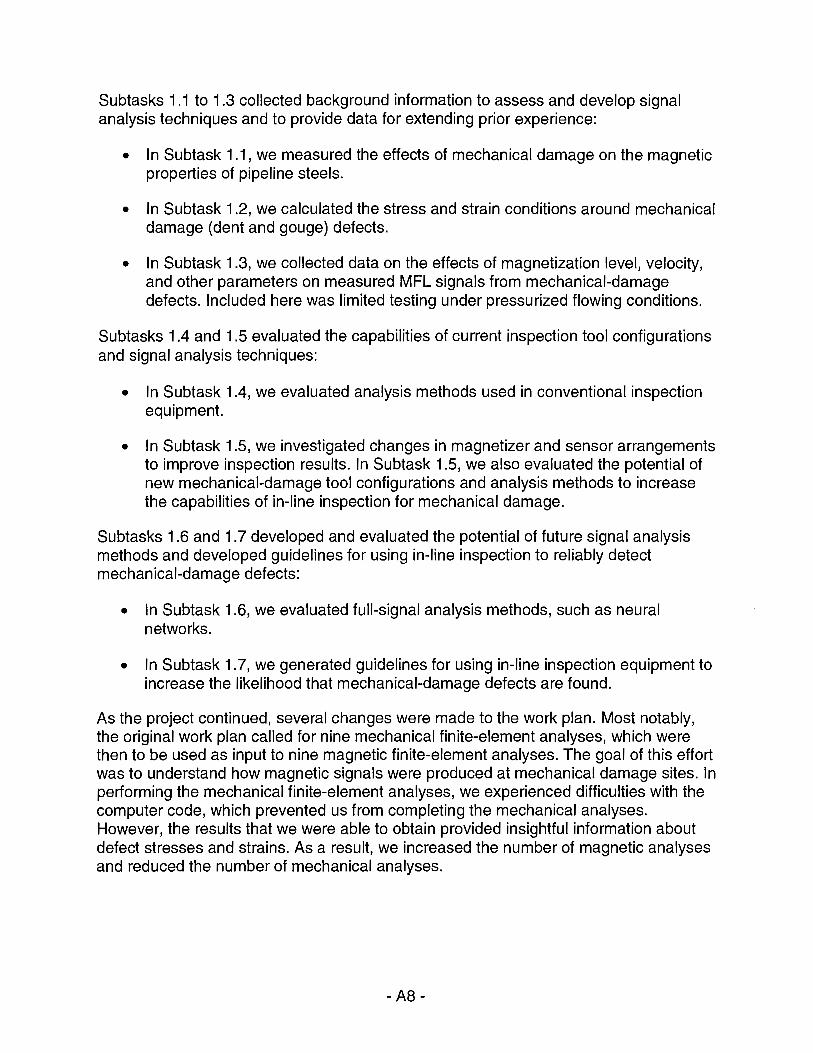
Subtasks 1 .1 to 1 .3 collected background information to assess and develop signal analysis techniques and to provide data for extending prior experience:

• In Subtask 1.1, we measured the effects of mechanical damage on the magnetic properties of pipeline steels.

• In Subtask 1.2, we calculated the stress and strain conditions around mechanical damage (dent and gouge) defects.

• In Subtask 1.3, we collected data on the effects of magnetization level, velocity, and other parameters on measured MFL signals from mechanical-damage defects. Included here was limited testing under pressurized flowing conditions.

Subtasks 1.4 and 1.5 evaluated the capabilities of current inspection tool configurations and signal analysis techniques:

• In Subtask 1.4, we evaluated analysis methods used in conventional inspection equipment.

• In Subtask 1.5, we investigated changes in magnetizer and sensor arrangements to improve inspection results. In Subtask 1.5, we also evaluated the potential of new mechanical-damage tool configurations and analysis methods to increase the capabilities of in-line inspection for mechanical damage.

Subtasks 1.6 and 1.7 developed and evaluated the potential of future signal analysis methods and developed guidelines for using in-line inspection to reliably detect mechanical-damage defects:

• In Subtask 1.6, we evaluated full-signal analysis methods, such as neural networks.

• In Subtask 1.7, we generated guidelines for using in-line inspection equipment to increase the likelihood that mechanical-damage defects are found.

As the project continued, several changes were made to the work plan. Most notably, the original work plan called for nine mechanical finite-element analyses, which were then to be used as input to nine magnetic finite-element analyses. The goal of this effort was to understand how magnetic signals were produced at mechanical damage sites. In performing the mechanical finite-element analyses, we experienced difficulties with the computer code, which prevented us from completing the mechanical analyses. However, the results that we were able to obtain provided insightful information about defect stresses and strains. As a result, we increased the number of magnetic analyses and reduced the number of mechanical analyses.

-AB -

Task 2 Workplan

Task 2 evaluated two inspection technologies for detecting cracks. The focus in Task 2 was on electromagnetic techniques that have been developed in recent years and that could be used on or as a modification to existing MFL tools. Ultrasonic techniques, while valuable, were not considered because they are the subject of research and development in ongoing GRI programs. Three subtasks were conducted to evaluate velocity-induced remote-field techniques, remote-field eddy-current techniques, and external techniques for sizing stress-corrosion cracks.

These subtasks were:

• Subtask 2.1. External Techniques for Sizing Stress-Corrosion Cracks.

• Subtask 2.2. Velocity-Induced Remote-Field Techniques.

• Subtask 2.3. Remote-Field Eddy-Current Techniques.

< suBtasR 2:2 · pc;it9•·1rtaus~a•·R~mrite#ield~.• mddifyJiOite:celement model L

tortlQ~fcr·· ya!p~t~ cµrJ~ntpefi4fb.at1on

Ff .. ~ndve!ociiy••ingµced•fi(;3Jds /

Task 2 Flowchart

There were no substantial changes to the work plan for Task 2 after the start of the project.

-A9 -

Background Material on MFL

The magnetic flux leakage (MFL) response to pipeline anomalies depends on many things, including the magnetic properties of pipeline steel and the geometry of the defects. Magnetic flux inspection tools locate pipeline defects by applying a magnetic field in the pipe wall and then sensing a local change in this applied field. As an example of this process, corrosion changes the ferromagnetic pipe steel into non­ferromagnetic iron oxide. An MFL inspection tool detects this change in magnetic property because it reduces the local ability of the pipe to carry magnetic flux.

Magnetic Flux Leakage

Detecting mechanical damage works on the same principle, but the changes in magnetic properties are more subtle. For mechanical damage defects, the flux leakage is due to a change in magnetic property induced by stress and plastic deformation rather than removed metal. These changes are much smaller and depend on the pipeline steel and the damage characteristics.

MFL Signals at Mechanical Damage

For more information on MFL, please refer to " Magnetic Flux Leakage (MFL) Technology for Natural Gas Pipeline Inspection"

-A10 -

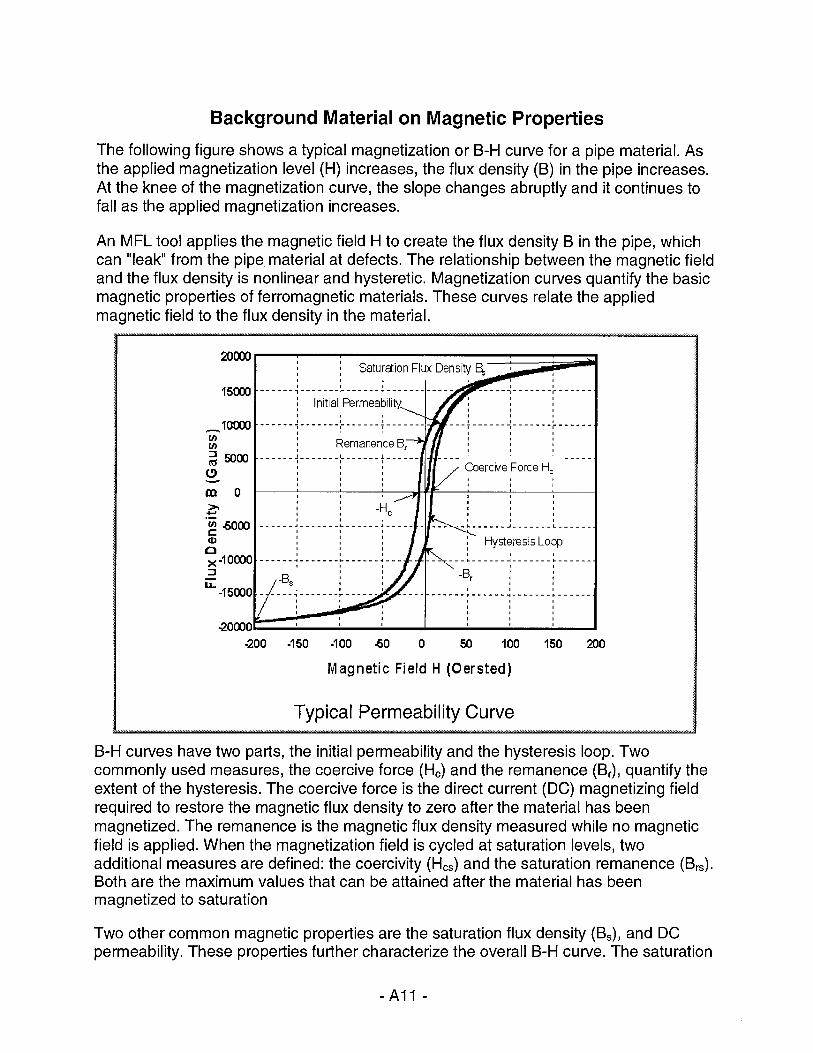
Background Material on Magnetic Properties

The following figure shows a typical magnetization or B-H curve for a pipe material. As the applied magnetization level (H) increases, the flux density (B) in the pipe increases. At the knee of the magnetization curve, the slope changes abruptly and it continues to fall as the applied magnetization increases.

An MFL tool applies the magnetic field H to create the flux density Bin the pipe, which can "leak" from the pipe material at defects. The relationship between the magnetic field and the flux density is nonlinear and hysteretic. Magnetization curves quantify the basic magnetic properties of ferromagnetic materials. These curves relate the applied magnetic field to the flux density in the material.

15(00

_1ocoo 1/) 1/)

~ 5000 (9

m o >, ..... ~ -6000

' ' ' . ' ' ' ' ' ' ' ------,--------------~------------ -----7-------r------: Initial Permeability ' ' ' ' ' ' ------ .-------, ------ .-------' . . ' ' ' ------ :-------: ------:------' ' ' ' ' ' ' ' ' ' ' '

' ' ' ' ' ' ' ' ' ' ' ---. ------ .-------, ------' ' ' ' ' ' ' ' ' ' ' ' Coercrve Force He

ID : Hysteresis Loop C : : : I I I

X -10000 - - - - - - ~ - - - - - - - ~ - - - - - - ~ - - - - - - - - - - • - - - - - - ~ - - - - - - - ~ - - - - - -::l I I -B t I

LL -Bs : : r : : ~5000 - ----~-------~------· -----------~------~-------~------

' ' ' ' ' ' ' ' ' ' ' ' -20000..._ _____ ......,. ________________ , -----·----' _ __,

-200 -150 -100 -60 0 50 100 150 200

Magnetic Field H (Oersted)

Typical Permeability Curve

B-H curves have two parts, the initial permeability and the hysteresis loop. Two commonly used measures, the coercive force (He) and the remanence (Br), quantify the extent of the hysteresis. The coercive force is the direct current (DC) magnetizing field required to restore the magnetic flux density to zero after the material has been magnetized. The remanence is the magnetic flux density measured while no magnetic field is applied. When the magnetization field is cycled at saturation levels, two additional measures are defined: the coercivity (Hes) and the saturation remanence (Brs), Both are the maximum values that can be attained after the material has been magnetized to saturation

Two other common magnetic properties are the saturation flux density (Bs), and DC permeability. These properties further characterize the overall B-H curve. The saturation

- A11 -

flux density has many practical and technical definitions. In this work, the saturation flux density is fundamentally defined as the flux density where changes in hysteresis behavior are negligible with changes in magnetizing field and arbitrarily defined as the flux density at a magnetic field of 200 Oersted. The DC permeability is a generic term used to represent the ratio of the magnetic flux density to the magnetic field. In this work, the incremental permeability (i.e., the slope of the magnetization curve) is used. The incremental permeability is the ratio of the change in magnetic flux density to the change in magnetic field (i.e., B/H).

For more detailed information on the magnetic properties of pipeline steels, refer to Variation of Magnetic Properties in Pipeline Steels.

-A12 -

Description of Typical Mechanical Damage Features

Mechanical damage is the largest cause of failures on gas-transmission pipelines today and a leading cause of failures on liquid lines. After a pipeline has been built, construction equipment (usually operated by outside parties) can deform the shape of a pipe, scrape away metal and coating, and change the mechanical properties of the steel. Sometimes this damage leads to immediate failure, and occasionally the damage leads to delayed or time-dependent failure. Obviously, immediate failures cannot be detected by periodic inspections. Consequently, a goal of this project is to detect those defects that might lead to delayed failure and differentiate them from benign defects.

Mechanical damage shows a number of features, such as:

(1) Denting

(2) Removal of metal at the surface of the pipe

(3) Cold-work of the material below the surface of the pipe and possible cracking in this area when the pipe is re-rounded by internal pressure

(4) Residual stresses and strains due to plastic deformation of the pipe wall

(5) Coating damage.

Mechanical Damage

The most significant of these features from the perspective of defect severity and the likelihood of delayed failure are the size and extent of the cold worked region. Dent depth, which can be easily measured by specific inspection tools, is not the most important parameter and is not sufficient to determine the severity of a mechanical damage defect. Movement or removal of metal by itself is usually not critical unless the amount of metal affected is more than about 10 percent of the wall thickness. Of course, removal or movement of metal is usually accompanied by cold working, so the presence of changes in wall thickness could indicate a significant defect.

-A13 -

Background Material on Magnetic Property Changes with Stress and Strain

The magnetic properties of pipeline steels are variable and a function of fabrication process, alloying agents, and microstructure. Stress and strain play major roles in defining a steel's magnetic properties. Previous work by SwRI and Battelle measured the effects of stress on a small set of pipe samples, but the effects of plastic deformation were not measured.

The following figure shows a typical magnetization curve or B-H curve for a pipe material. As the applied magnetization level (H) increases, the flux density (B) in the pipe increases. At the knee of the magnetization curve, the slope changes abruptly and it continues to fall as the applied magnetization increases.

Adding stress or strain changes the shape of the magnetization curve. Compressive stress shifts the curve upward in the region of the knee, but it has little effect for higher magnetization levels. As a result, an MFL signal at a mechanical damage defect changes with magnetization level. At very high levels, there is almost no effect of stress and the signal is primarily due to the geometry of the defect. At low levels, the signal has both geometric and stress components.

Pipe grade, such as API grade X52, is not a measure of magnetic properties. Many fabrication processes and concentration of alloying elements can produce pipe of a particular grade but with different magnetic properties. Depending on the fabrication process, the magnetic properties can be anisotropic and a function of circumferential location with respect to the longitudinal seam weld.

"' C 0

16 " 'al C CJ)

"' ::a:

High Magnetization Level Signal

Magnetizing Field ( H)

Effects of stress on magnetization curves

For more detailed information on the magnetic properties of pipeline steels, refer to "Variation of Magnetic Properties in Pipeline Steels "

- A14 -

Comparison of MFL Signals for Metal Loss, Dents, and Cold Work

MFL is capable of detecting mechanical damage components such as simple dents, cold work, residual stresses/strains, and removed metal. Part of the signal generated at a mechanical damage defect is due to geometric changes - for example, a reduction in wall thickness due to metal loss causes flux to leak out. Some of the signal is due to the separation of the sensor from the pipe (lift-off), which can be minimized by a good sensor carrier system. The rest of the signal is largely due to magnetic changes, for example, changes in magnetization properties that result from stresses, strains, or damage to the microstructure of the steel.

MFL signals for metal loss, dents, cold work, residual stresses, and plastic strains are fundamentally different. These differences can be seen in the experimental MFL signals shown below. The signals correspond to the axial component of the MFL field as measured by a Hall-effect sensor.

REMOVED METAL DENT GOUGE

MFL signals at mechanical damage

The plot on the left is a typical MFL signal from metal loss. Flux, which is normally carried by the pipe wall, "leaks" in regions where the wall thickness is reduced. The sensor records an increase in flux level at the reduced-thickness area. Metal loss signals have a characteristic increase in measured field along the defect, with a slight decrease at both ends. For very long defects, there can be a dip in the signal in the center part of the defect.

The plot in the center is a typical MFL signal from a dent. Here, the signal shape is fundamentally different than that seen at metal loss. The signal is due to two effects that occur at the same time. First, the sensor orientation relative to the local pipe wall changes. The sensor still records the axial field but the pipe wall is no longer parallel to the sensor; since the flux field is a vector quantity, the resultant measurement changes. Second, residual stresses and strains change the local magnetic properties. Dent signals show characteristic peaks near the start and finish of the dent with a relatively low signal through the defect.

-A15 -

The plot on the right is a typical MFL signal from a cold worked region. Here, the signal shape is fundamentally different from that of both metal loss or a dent. Flux in the region immediately below the cold worked area decreases. This change occurs because the cold worked region, which is on the side opposite the sensor, carries more flux, thereby reducing the flux in the rest of the pipe. In addition, there is a slight increase in signal at either end. These two signal features are characteristic of mechanical damage.

For more detailed information on MFL signals from mechanical damage, refer to "The Feasibility of Magnetic Flux Leakage In-Line Inspection as a Method to Detect and Characterize Mechanical Damage."

-A16 -

Linear Test Rig Description

The linear test rig is a moveable platform for testing inspection technologies, including MFL systems, at typical inspection velocities. The inspection platform is pulled along a 24-foot guide rail either through a full diameter pipe or under a partial diameter pipe section. Tests conducted under this program used flat plates or a partial diameter pipe section that represented an arc of approximately 120 degrees.

Linear Test Rig

For more information on the linear test rig, refer to GRI Pipeline Simulation Facility Nondestructive Evaluation Laboratory.

-A17 -

Pull Rig Description

The pull rig is a set of four pipe runs through which in-line inspection tools can be pulled. Each pipe run is 300 feet long and contains three 80-foot replaceable defect sections. Mechanical damage and other defect sets are mounted in the replaceable sections and data are taken using the MFL test bed vehicle. Pulls can be made at velocities up to approximately 25 miles per hour.

Pull Rig

For more information on the pull rig and its defect sets, refer to GRI Pipeline Simulation Facility Pull Rig, GRI Pipeline Simulation Facility Metal Loss Defect Set, and GRI Pipeline Simulation Facility Stress Corrosion Cracking Defect Set.

- A18 -

Description of Basic Material Property Testing

An understanding of the effects of stress and strain on magnetic properties for a wide range of materials is needed to determine whether MFL can be used to reliably detect mechanical damage. During the initial planning of the flow loop and as part of Battelle's pipe research program, 40 joints of different pipe materials were removed from service by various pipeline companies and provided to Battelle. These materials had been characterized mechanically for stress-strain and toughness properties and chemically for composition. A total of 36 joints were further characterized magnetically in this project.

The characterization and evaluation had three goals. The first was to determine whether there were clear correlations between magnetic properties and mechanical properties. The second was to determine whether magnetic properties change significantly with the application of tensile or compressive stresses and strains. The final goal was to assemble a database of both magnetic and mechanical properties for future developmental activities. Each of these goals was met.

The 36 samples were magnetically characterized following ASTM Standard A 773-80. This method, illustrated below, uses a ring sample machined to have an outside diameter of 2.0 inches and a square cross section of 0.15 inches. This provides an inside diameter to outside diameter ratio of 85 percent, as required by the ASTM standard. To obtain this sample geometry from the pipe material, a 6-inch by 6-inch coupon was cut from the pipe opposite the seam weld. The 2-inch ring sample was machined from this coupon in a liquid bath to minimize the effect of sample preparation on the magnetic properties.

The ASTM experimental procedure specifies that each ring sample be wound with drive and sense windings. The drive winding, used to generate the magnetic field (H), has a minimum of 140 turns to generate a field strength of 200 Oersted. The sense winding, used to measure the change in flux, has a minimum of 80 turns to attain accurate measurements. The windings were applied by hand, and a few additional turns were added when space was available. Measurements were made using a LDJ model 3500H Hysteresisgraph. Sufficient current was applied to the drive windings to produce 200 Oersted. After demagnetization, the magnetic field and flux density were digitally recorded at increments of nominally 0.2 Oersted for the initial magnetization curve and 0.5 Oersted increments for the hysteresis loop.

ASTM test sample

-A19 -

Description of Material Property Stress Tests

Magnetic properties of 12 of samples were further examined under tensile and compressive loading with up to 8 percent plastic deformation. Two sample configurations were used to measure magnetic properties: a "dogbone" shape for tensile loading and a thin cylinder for compressive loads. The compression sample required special attention to prevent buckling when under load. Two coaxial cylinders were used to support the sample during compression. The central holes in these cylinders were sized so that they could be slipped smoothly over each end of the sample. Very small clearances were used to prevent lateral buckling of the sample. The sensed area, in the center of the sample, was exposed between the larger coaxial cylinders.

Each sample was prepared with strain gages and with an encircling coil to measure magnetic flux. Hall probes in_ the vicinity of the sensing area were used to measure the magnetizing force. A large magnetizing coil was placed over the whole arrangement, and load cells within the loading linkage were provided as an alternative measure of specimen loading.

Test Procedure

Each sample was mounted in the test fixture, which has a scissors-type loading linkage under manual adjustment. A computer-driven magnetic sensing system automatically cycled the magnetic excitation field and collected the data from all sensors. Strain gages were connected to a bridge circuit and read manually.

B-H curve data were collected for each tensile specimen under a half-dozen different applied loads. Each sample was taken to mechanical yielding, and 8-H data were collected again for 1 percent plastic deformation plus a range of applied elastic loads. The sample was then further yielded to 2 percent, and the applied loads were cycled again. The process was repeated to a maximum of 5 to 8 percent plastic deformation. A similar process was carried out with the compressive samples.

-A20 -

Description of Full Pipe Tests

Magnetic properties vary within a pipe. To examine the magnetic properties on a full section of pipe, magnetization curves were measured around the circumference of two pipes under tensile and compressive loading. The following figures shows the arrangement of the test sample.

5

Test Setup for Measuring Full-Pipe Variations in Stress Effects

Table of Measured Material Property Variations

NO LOAD TENSION COMPRESS MEAN 6.7 7.7 7.4 9.7 std Dev 1.2 0.55 0.8 0.9 MAX 9 8.6 8.4 10.9 MIN 4.5 7.1 6.3 8.5

MEAN 1003 1297 1425 488 std Dev 331 142 75 28 MAX 2090 1497 1521 549 MIN 580 1101 1325 462

The coercive force is given in Oersteds. The permeability is given as the maximum relative permeability.

For more detailed information on the magnetic properties of pipeline steels, refer to Variation of Magnetic Properties in Pipeline Steels.

-A21 -

Typical Database Entry

Material 24-06

t 0

Si -S Q ~ -10

U.. -1S

.2,)

-100

0

0

2000

/ I

J

/'/ I

t j I I

J, //

0

M:a{Jletizitl] Force H (Oersted)

. .,,,..,-~

100

M:a{Jletizitl] Force H (Oersted)

/ ' $' I Q 1SOO !£.

1 00X Pi era + Nita I B:ch O 8336 ~ = 1000

The mi crostn.clure is som e\l\hat banc:ed i and consists of a mi>ture of tetrite and ~ pearlite wth perhaps some banite. Tre S soo steel e>tlibitsa duplex grain sze Vli'lhthe c. liner grains having a grain size of .AS1M 11 and the larger ferrite grains having a o grain size of .AST M 8.5. It appears thct o this s:eel may have been cortrolled rolled wth a lowlinisling terrperature.

I I I

I I

/

-A22 -

\ \ \ \_

~ :'-....,____

~

10 lO

M:a{Jletizitl] Force H (Oersted)

100

-

=

-

Additional Details on the Linear Test Rig Experiments and Defect Sets

The linear test rig was used to take data for a variety of materials and defects. Some edge effects are present when using the linear test rig, but in general, these effects were small. The measurement system used to record data is modeled after that used in the test bed vehicle. So, the resolution and accuracy of measurements from the pull rig should be the same as that from the linear test rig.

For this program, measurements were made at velocities under about 3 miles per hour. Prior results show that such velocities are low enough that they should have negligible effects on the inspection signals. Typically, data were taken at 1 O Oersted intervals, ranging from as low as 10 Oersted to as high as 150 Oersted. In addition, remanent measurements were taken using no applied field.

Three types of defects were used in the linear test rig: fifteen defects made under pressure, five natural dent defects in pipe removed from service, and twelve simple mechanical damage defects made in flat plates. The defects consisted of plain dents, cold worked regions, dents with cold worked regions, and cold worked regions with removed metal.

Additional linear test rig defects were made in two pipe steels: the flow loop material and a generic X52 material. The materials used are the same as those used for the pull rig defects.

iilllinear Test Rig Defect Tables (Partial)

m.lLayout of Defects in One Defect Set

For more information on the linear test rig, refer to GRI Pipeline Simulation Facility Nondestructive Evaluation Laboratory.

-A23 -

Linear Test Rig Defect Tables (Partial)

·mnElldts~r·ir•FABRJGATEO.DEi=ECTs•i) ·· ion

~2W5~rit, ?llj.~i~?1•iJct~ht~; . nth oent(Roi.1nded

.:::::::::::::· .. :. .:.::::: .. :.:.·::.::·· ... ·.::::::·:· ..... .

·inp.~ .•• ~crabe: ~.~ieciM.etal,.Littl~[)~nfihg•••·······.· .• ,Finch Stt~pe; Moved Me haliow Da'ltjng . .

G08,8: • H~rd $P~i0i'4 Scfafah

D·0t > 0.45-inch 0,02 gouge Wt D-03

0~04

>8·01

•··•···•.·g;(jJ

Layout of Defects in One Defect Set

TOPVIEW I WELD

MAGNETIZER VELOCITY ---t/11- SMOOTH DENT,

\ t DENT SCRAPE ,, ·

-- - - - - - - - - - - - - -- -- - - - - - -- -- ""'"-- - -- - - - - - - - - - - - - - - - - - -- - - -- -- - -2' -SMALL -iii (i;. w, GOUGE --2,;~-u:E-- --- --------~}--- ---@-~-~~~~~~~~.----------

scRAPE SCRAPES

-A24-

Typical LTR Data

...... -.... ·. 30·-l· -----l-----l'------ll----1----1----1----+----_._ ___ _._ __ --I

::~:TE: Low MagLevel ::::: -----.---- ........ ,- ":"'":"'-· ....... ,.:.· ......... ::·::-.':._ ....... - ·:·:···: ·: :._:·· .·· ....... - ... - ............. ... ~.· 20.-+-----i----+----i-----+----t-----+_-_-_-. -.. --.-.-_-t_-_-_-_-_-.-_-_-t_-_-_-_-_-_-. -t_-_-_-_-_-_-. -1

£ ··.. ---~~~~-----~:------~ ------. ro. ..;.·..;.·._ :., ... ,_. ~ "':"--:--:- --·-:- -.:. ~- .:.'~'~:~-~ ~-~-.:. ·:·:-~-~ :': ~ .:..:. : ·: ::: : : : : ; ·~ 10+-_-_-.. _-. _-. _-.-"+. -._-_-_-_-_-_-.. !----+-----+._-. _-.-_-_-_-._-.+-_-_-. _-. _-.---..• -. +-_-·: _-.:-_-_-_-. -.+.-.;-. --·: _-.-_-_-_+_-._-.-_-.-._-_-_+-_-_-_-._-.-_.--!_ 00. ...J L1.

. . . . . . . . . . . . . . : .

---,----~~-~~--➔~-------------___ ,· .··.· .· ---- ·--·--·------. ------··;:i; o+------t----+---+------t-. -----t.~---+-++-+------t.,....--+----l

_..:;.,.,;,

.· . . . . . . .. ---------------------------------. .. .. . . .. . ... v~------·-------.------- -----~~---------- .-------------------·. -30;.L: ----'------'-----'-----''------''-----'-----'------'------'-------'

145 151 1fil 155 157 100 161 163 11:6

Sensor Position.(hchesJ

-A25 -

Additional Details on the Pull Rig Defects

Two types of defects were used in the pull rig. These defects included 38 defects made on pressurized pipe samples and 32 defects made by hitting pressurized flow loop pipe with a backhoe. The pull rig defects included dent depths up to 6 percent of the pipe diameter. Gouge depths range from nearly zero to 25 percent of the wall thickness, and gouge lengths range from nearly zero to 6 inches. c!:Defect Installation.

Typical dent

The pull rig defects were installed in two pipe samples, representing an X42 and X65 steel, which were removed from service and donated to the program. lPull rig defect sets.

Data were taken with Hall-effect sensors spaced on 0.33-inch centers circumferentially and after each 0.1 inch axial travel. The raw data were collected in a series of data files and are available for use with a customized viewing program. In addition, individual defect files were created for each run, and a separate viewing program developed that allows comparisons of measurements from up to four defects.

For more information on the pull rig and its defect sets, refer to GRI Pipeline Simulation Facility Pull Rig, GRI Pipeline Simulation Facility Metal Loss Defect Set, and GRI Pipeline Simulation Facility Stress Corrosion Cracking Defect Set

-A26-

Defect Installation

A machine is available at Battelle for making mechanical damage defects such as dents and gouges. This machine has two hydraulic actuators to press a tool into the pipe. The vertical actuator applies radial compression on the pipe, and horizontal actuator pushes the tool along the pipe axis. The machine can accept different indentor types, enabling the simulation of many defect types and controlling the defect geometry.

For defects made while there is internal pressure in the pipe, the defect rerounds when the indentor is retracted. This rerounding can significantly change the stress distribution in the defect regions. The following links provide video clips of defects being produced. The small video links are typically 100 to 300 Kilobytes in size; the large links are between 1 and 6 Megabytes in size.

Dent & Gouge Machine Photos #1 and #2

-A27-

Dent & Gouge Installation Photos #1, #2, and #3

-A28 -

Resulting Dent and Signal

Low Magnetiza:i on Level High Magnetiza:ion Level

·u

0 ~) 5 1,.., ,. 15

Resulting Scrape

Resulting Dent and Gouge

-A29 -

Resulting Scrape

Resulting Scrape and MFL Signal

150 160 170

Axial Distance (Inches)

Resulting Hit and MFL Signal

9) 9< ;:L 96 ss ·100 1~ Ic.4 ·10& ·o:: no 1-i2 1·4 ·IE 110 120

Axial Distance (inches)

-A30-

61 57

53

.Jg ., 41 :J7

33

j7

13

Resulting Multiple Hits and MFL Signals

1,0 122 124 ll6 128 130 132 134 136 1;8 ·4: 1'2 W '4€ 148 1,0

Axial Distance (inches)

Resulting Multiple Scrapes and MFL Signals

m m ~ m m ~ m ~ ~ ~ m ~ ~ ~ ~ n Axial Distance jinches)

-A31 -

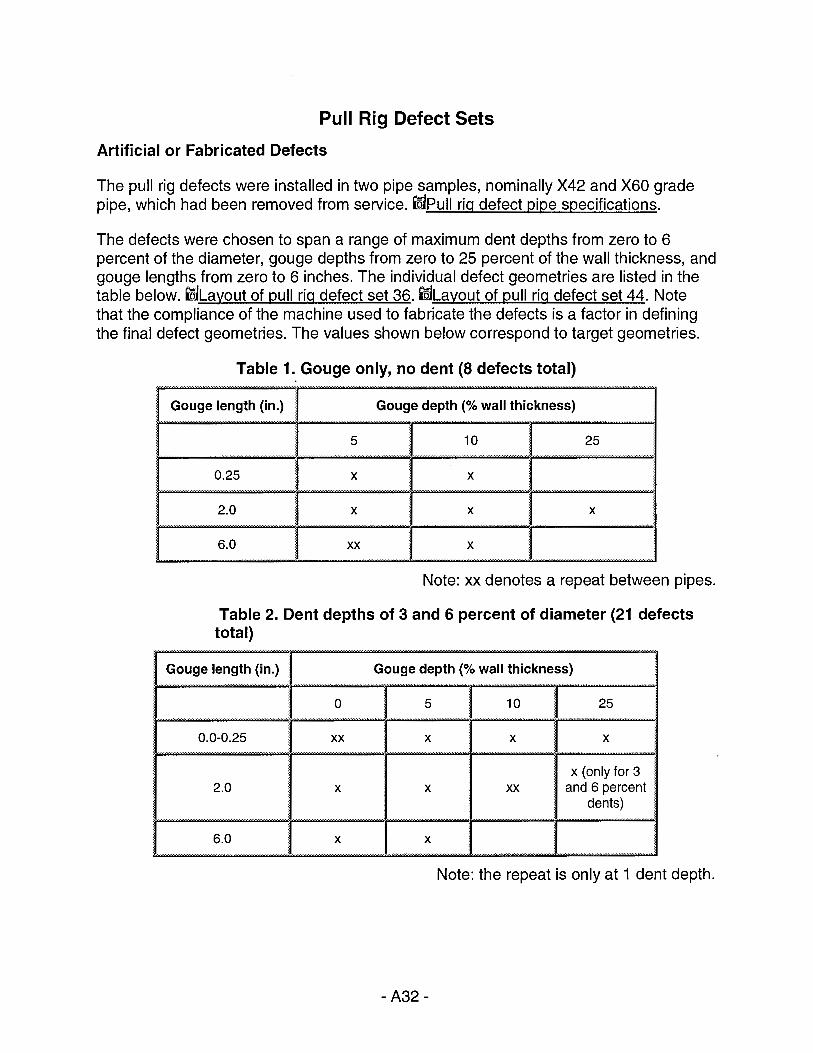
Pull Rig Defect Sets

Artificial or Fabricated Defects

The pull rig defects were installed in two pipe samples, nominally X42 and X60 grade pipe, which had been removed from service. imPull rig defect pipe specifications.

The defects were chosen to span a range of maximum dent depths from zero to 6 percent of the diameter, gouge depths from zero to 25 percent of the wall thickness, and gouge lengths from zero to 6 inches. The individual defect geometries are listed in the table below. iilllayout of pull rig defect set 36. iillLayout of pull rig defect set 44. Note that the compliance of the machine used to fabricate the defects is a factor in defining the final defect geometries. The values shown below correspond to target geometries.

-Table 1. Gouge only, no dent (8 defects total)

,_ :_ ,::,.h (in.) Gouge depth (% wall thickness)

5 10 25

0.25 X X

2.0 X X X

6.0 xx X

Note: xx denotes a repeat between pipes.

Table 2. Dent depths of 3 and 6 percent of diameter (21 defects total)

Gn11nP lenoth (in.) - - Gouge depth (% wall thickness)

0 5 10 25

0.0-0.25 xx X X X

x (only for 3 2.0 X X xx and 6 percent

dents)

6.0 X X

Note: the repeat is only at 1 dent depth.

-A32 -

Table 3. Radius cutter and dent to 3 and 6 percent of diameter (9 defects total)

Gouge length (in.) Gouge depth (% wall thickness)

5 10

2.0 X X

6.0 xx X

Note: the repeat is only at 1 dent depth.

Defects Created by Backhoe

In addition to the fabricated defects shown above, we installed a set of mechanical damage defects that had been made by a backhoe in a Gas Research Institute project on real-time monitoring. This pipe sample includes the following defect classes:

• Vertical hits on crown of pipe

• Hits and scrapes on crown of pipe

• Scrapes on crown of pipe

• Hits and scrapes on side of pipe

• Scrapes on side of pipe

• Scrape perpendicular to pipe axis.

These defects were made by striking the pipe with a rubber-tired 3000 series John Deere backhoe. Two internal pressures were used during impact, 150 psi and 250 psi.

-A33 -

Weld

270 -

180 -

90 -

Weld 0

Defect Pipe Specification

PULL RIG DEFECT PIPE SPECIFICATIONS

Defect Set in Pipe #36

Dent Depth (%diameter) x Gouge Length (inches) x Gouge Depth (%wall thickness)

~ 0% dent Depth CD 3% dent Depth 6% dent Depth e, Natural Dent

I I

- - - ~ - - - - ~4 :,- - ~ - - - -:- - - -~ - - - ~ - - - ; - - - -:- - - - ~ - - - ~ - - - - ~ - - - -:- - - - ~ - - - ~ - - - -f :i9 I : #35 : I #~4 I

6%x. 25x5• 6%x6x1•0 , 6%xi2x1 0 , I I I I I I I

I I I I I I I I I I

- - -~-~ - - - ~ <GiISi-~- - - -f!\- - - ~- - - - ~ - <0 (./:t;;;.,'.'::, - ~ -~~- - - - ~ ®- ~ - - - -!.- - - ~ - - -~- - - -: #28: : #31 ' =134 ' #27 #!O : #43: : #46 : )J%x2x:Z5 6%x2x1 OR 3%½0.25x5 3%x1x5R ' 3%>l6x5 )J%x2X5 6%l<0.25x:Z5

---~----~~--:- r-- ~-- - -,- - - I -, •»~ii'':io:Y\P- - ~ - -E}~ - - - ~ - - - -:- - - -1 :#3□: :#33: :#36 I #39 I 'll142 #4p I #48 I I

20

3C)f,x6x1 QR 6~0.25*1 O 0%)<6x5: 6%:px5R: 3%)<2xO : 3%x6t5R ~%x0.~5x25

40 60 80 100 120 140 160 180 200 220 240 260 280 JOO 320 340

Axial Distance (inches)

-A34-

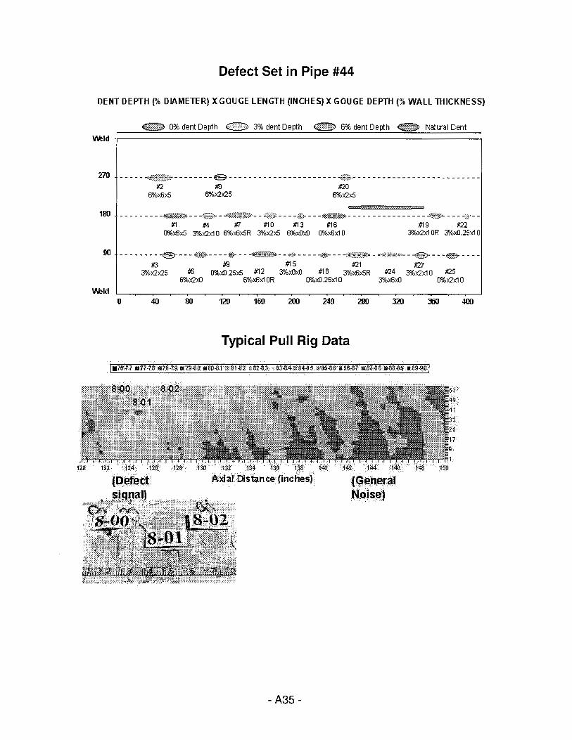
Defect Set in Pipe #44

DENT DEPTH{% DIAMETER) XGOUGE LENGTH (INCHES) X GOUGE DEPTH(% WALL THICKNESS)

~ 0% dent Depth c:::::::;i 3% dent Depth ~ 6% dent Depth ..m., Natural Dent "1\eld -.---------------------------------,

270 - - - - - . ,,:;\Flt:±!+•,., - - - - - - - - S - - - - - - - - - - - - - - - - - - - - - - ""#ii!F- - - - - - - - - - - - - - - - - - - - - - - - - -1/:2 1113 1/:20

6%x6x5 6%x2x25 6%x2x5

3§,.)fW, .......... , ........ , ........ .,.. ... .

180 - - - - - - - - -~+4W~- - -~~ - .. :AAf:@l'.#}~Ji1·- - :i,(_:~r~'- - - -Bl}- - - -~- - - - - - - - - - - - - - - - -t~~).. - - - -(i:=- -tf1 #4 tr1 tf10 tf13 tf16 tf19 1/:22

O¾x6x5 3%x2x1 O 6%x6x5R 3%x2x5 6%);f));f) O¾x6x1 0 3%x2x1 OR 3%);f).25x10

90 ---------e----<>----e,,..-~-- •·••.·----$---~z:YT::::cc- ··.·. >-- ... :::::z:i ---czr,----

W!ld 0

#3 t13 tf15 1/:21 1/:27 3%x2x25 #6 O¾);f) .25x5 tf12 3%);f));f) tf18 3%x6x5R 1/:24 3%x2x1 O 1/:25

6%x2);f) 6%x6x1 OR O¾);f).25x10 3%x6);f) O¾x2x10

40 80 120 160 200 240

Typical Pull Rig Data

. ;,;32 134 13~ ., . j~~ •·•. Axial Distance finches)

-A35 -

280 320

(.~~11eral .Ne>is~)

360 400

Description of the MFL Test Bed Vehicle

The MFL test bed vehicle (TBV) was built as a test platform for use in the Pipeline Simulation Facility. This vehicle eliminates the need to develop a test platform for this research program on mechanical damage. The test bed vehicle makes it easier for research to attain field realism, which is something only vendor laboratories had been able to do previously.

General Description

MFL tools for pipeline inspections are completely self-contained units containing magnets, sensors, data conditioning and recording systems, and power systems. The systems used in most MFL tools include:

• A drive system, which is used to propel the tool through the line. Differential pressure acting on the drive system pulls the tool through the pipeline.

• A power system, which provides battery power for the sensor, data conditioning and recording systems.

• A magnetization system for magnetizing the pipe.

• A sensor system, used to measure a flux-leakage signal.

• A data conditioning and recording system, which amplifies, filters, and stores the measured signals.

The magnetic flux leakage (MFL) test bed vehicle (TBV) was designed to simulate current inspection technology as well advance the state of the art of this technology. Many components were designed so that different configurations could be achieved. A photograph of the three module test bed vehicle is shown below. The overall length is approximately 12 feet and it is configured for 24 inch diameter pipe. The three modules are the

• Propulsion/ Battery module

• Magnetizer and sensor module

• Electronics module

-A36-

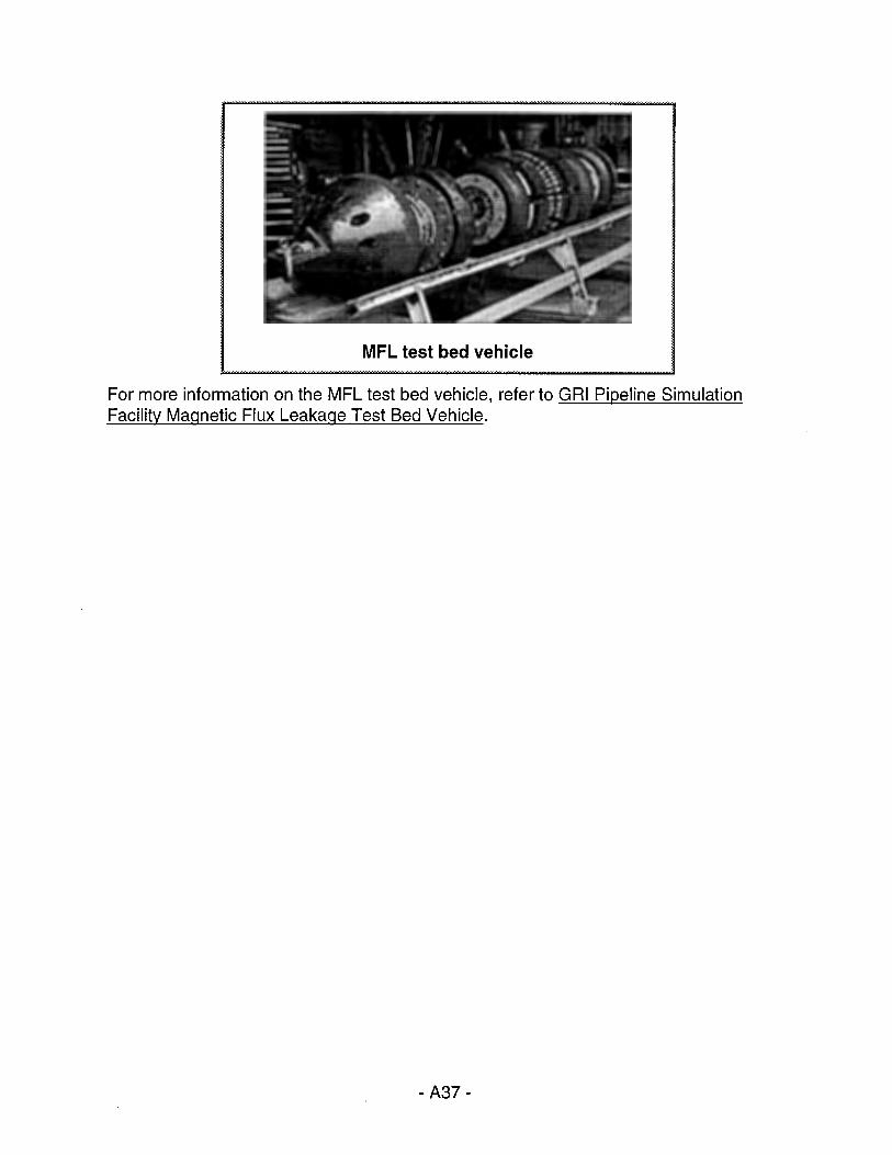
MFL test bed vehicle

For more information on the MFL test bed vehicle, refer to GRI Pipeline Simulation Facility Magnetic Flux Leakage Test Bed Vehicle.

-A37-

Additional Details on the Test Bed Vehicle Modifications

Magnetizer Modifications

An MFL tool contains a system that magnetizes a length of the pipe wall. Typically, sets of magnets are used to provide coverage around the circumference of a pipe. A permanent-magnetic system, shown below, has pairs of magnets that are attached to backing bars and to metal brushes or magnet shoes that rub against the pipe wall. Ferromagnetic brushes are used to efficiently couple the magnetic field to the pipe body. The backing bar is made of a material that is selected to obtain a high flux level in the pipe wall.

Permanent-magnetic system

The original magnetizer produced field levels in typical wall thickness pipes ranging from 70 Oe to 110 Oe. The magnetizer had 28 megagauss-oersted neodymium-iron­boron magnets in eight magnet assemblies spaced around the circumference. Each assembly had 18 sq. inches of NdBFe magnets and brushes for coupling the magnetic energy into the pipe. (See aruBackground information on magnet strength.)

Linear test rig results showed that two magnetization levels are required: one higher and one lower than the field levels established by the original magnetizer. For optimal characterization, the low field level should be between 50 and 70 Oe, and the high field level should be above 150 Oe. To attain the lower magnetization level in the pipe, some of the magnetic field was coupled directly to the backing bars by shunts. To attain higher magnetization levels in the pipe, the magnet areas were increased by 8 square inches using NdBFe 35 magnets.

Sensor Modifications

Sensors between the magnet pole pieces measure the flux leakage field. (See am Background information on MFL sensors.) The purpose of sensor systems is to convert the flux leakage field into a signal that can be stored and analyzed. The sensor system

-A38-

consists of the sensors themselves, the mounting system used to support the sensors, wear plates between the sensors and the pipe, and cabling between the sensors.

Sensors

The test bed vehicle has 48 sensor heads, six on each magnet bar. Each sensor head has four axial hall element sensors. The configuration of these sensors is shown below. Sensor spacing is similar to commercial high resolution systems. To minimize noise, some amplification of the signal takes place very near the sensor.

Sensor boards

All sensors on the test bed vehicle were replaced by SS495 Series, solid-state, ratiometric, linear sensors manufactured by Honeywell Micro Switch. These sensors have the necessary characteristics to measure the fields generated by mechanical damage defects. The sensors operate on supply voltages ranging from 4.5 volts to 10.5 volts. Outputs are ratiometric, and are set by the supply voltage. The sensors measure a minimum of +/- 600 Gauss, and they include an amplifier integrated into the circuit. Sensor arrays made up of multiple sensors are constructed using printed wiring boards. These sensor arrays are potted in a sensor housing and mounted in the sensor.

Electronics Module Replacement

The electronics module of the test bed vehicle was designed to collect data during pull rig and flow loop tests. The unit has both sensor electronics and digital computer recording capability. There are approximately 4.3 million square inches of pipe surface in the flow loop. If data are recorded in 0.1 inch (5 mm) intervals in the axial direction and using only the axial sensors, approximately 100 million data points would be taken

-A39 -

each lap. The original electronics module was not designed to handle such large amounts of data.

The electronic components were replaced with a personal computer compatible system using PC-104 format cards to minimize size and maximize ruggedness. The computer module shown below has a central processor unit (CPU) card, with six analog-to-digital (AID) cards, and a power supply module. A mass storage device and cabling complete the data acquisition system.

Po-wet supply

486:S.XCPU

A.nalogto DiQital Converters

Electronics module

CPU: The CPU module controls the functions of the data acquisition system. A Real Time Devices CPU module, model number CMi486sxlc66, is representative of the CPU to be used for the control computer. This machine utilizes a 486sx class processor running at 66 MHz, and provides sufficient computing power for the recording of flux leakage signals.

AID Converters: The AID converter hardware converts the analog signals from the sensors into digital signals that can be stored by the computer. There is one AID channel for each of the 192 sensors. Sensor voltages are in the range of 0 to 10 volts. Using a 16-bit converter allows 65536 discrete voltage levels to be measured, equating to 0.15 mV per bit. This resolution allows meaningful measurements of magnetic field strength to be recorded for later analysis. The respective AID channel captures the data from 96 sensors, the 96 AID channels being achieved by using six AID cards, each with 16 input channels.

Two separate data recording modules running in parallel are used to record the output of all 192 sensors. The 16 bits of data for each channel is in 2-byte words on the mass storage device. Each storage record, containing one data sample from each sensor, contains 192 bytes of information. Representative 16-channel, 16-bit AID PC104 cards are the PC104-DAS16JR converter boards manufactured by Computer Boards, Inc. The digital sensitivity of the sensor is approximated 0.1 gauss per quantum level.

-A40-

Mass Storage: Coupled to the CPU is a mass storage device to store the control software and the acquired data. It is a solid-state disk drive, AT2500-192, manufactured by MemTech, Sunnyvale, CA. This solid-state storage device uses Flash memory as the storage elements, and includes a standard IDE interface. Using non-volatile memory configured to have the standard disk interface results in a rugged storage device with no development of custom hardware.

Storage drive

The CPU, AID converters, power converters and mass storage devices are mounted in a rugged frame. The assembled test bed vehicle data recorder is shown below. Testing has shown that data from all 192 sensors can be recorded in 0.1 inch increments at speeds up to 8 miles per hour.

Overall system

Data Display Software

The data recorded by the MFL test bed vehicle can be displayed using a proprietary Windows® based viewer. The following figure shows test bed vehicle data recorded in the pull rig with the mechanical damage defect set. In a typical display, both image data

-A41 -

and a particular sensor output are displayed. For the image display, axial distance along the pipe is on the horizontal axis. Each horizontal line represents one sensor with color corresponding to flux leakage amplitude.

Display software

-A42 -

Background Information on Magnet Strength

Various permanent magnet strengths are available. A magnet's strength is categorized by its maximum energy product, which is a measure of the magnet's force of attraction. Many older inspection systems used ceramic permanent magnets, which have an energy product of 1 to 4 megagauss-oersted.(10) Other systems used Alnico (aluminum-nickel-cobalt) magnets, which have energy products from 5 to 12 megagauss-oersted. Rare earth magnets, such as neodymium-iron-boron magnets and samarium-cobalt, became available in 1984. These magnets have energy products from 18 to 45 megagauss-oersted. Thus, the newer magnets have dramatically increased the magnet power available. They are also mechanically stronger than the other magnet types, which tend to be brittle, and they are significantly more expensive.

Background Information on MFL Sensors

The two types of sensors commonly used in MFL tools are induction coils and Hall elements (field sensor). Coils measure the rate of change of a magnetic field, while Hall elements measure the actual magnetic field strength. Historically, induction coils have been the most commonly used type of sensor on MFL inspection tools because they do not require a power source. Instead, a voltage is generated in a passive coil of wire or printed circuit as it passes through a changing magnetic field. A recording device measures this voltage, which is proportional to the change in flux density. Since a coil responds to a change in flux density, the output of a coil is a function of the speed at which it is moving. Integration techniques can be used to convert coil measurements to flux density measurements, but the constant component is lost. The constant component is needed to determine the applied magnetic field strength.

The MFL test bed vehicle uses Hall elements. In a Hall element, an electrical current is distorted by the presence of a magnetic field. A recording device measures the change, which is proportional to the strength of the magnetic field and the amount of current. Although electrical power is required to generate the current, Hall elements are not sensitive to speed, which makes them attractive for research applications. Also, the constant field component that is related to the applied flux density in the pipe is available.

Sensors are spring-loaded against the pipe surface. The test bed vehicle has a spring­loaded four-bar linkage system. Spring loading allows the sensors to ride over weld beads, dents, and other intrusions. The stiffness of the mounting system and the mass of the sensors affect how closely the sensors follow the wall. Stiff systems closely follow the wall, but they also increase wear on the sensors. Low-mass sensors follow the wall better than high-mass sensors, but there is often a trade-off between sensor mass and sensor ruggedness.

-A43-

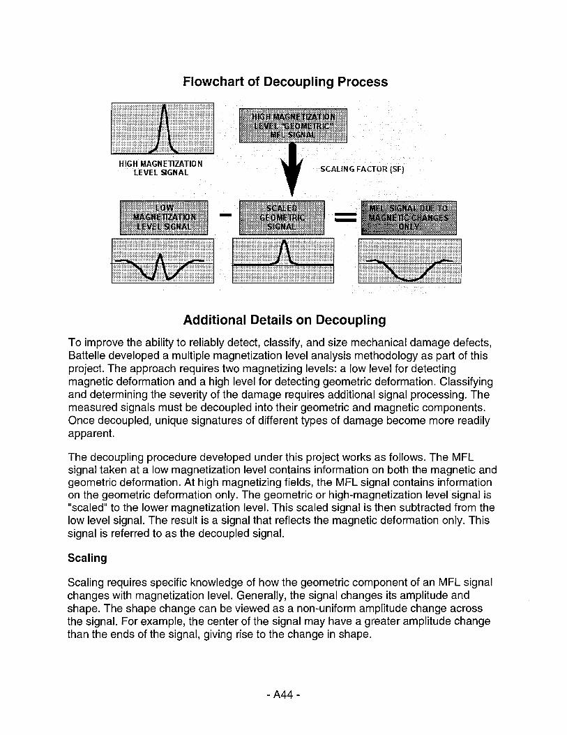
Flowchart of Decoupling Process

HIGH MAGNETIZATION LEVEL S1GNAL

-SCALING FACTOR (SF)

--

Additional Details on Decoupling

To improve the ability to reliably detect, classify, and size mechanical damage defects, Battelle developed a multiple magnetization level analysis methodology as part of this project. The approach requires two magnetizing levels: a low level for detecting magnetic deformation and a high level for detecting geometric deformation. Classifying and determining the severity of the damage requires additional signal processing. The measured signals must be decoupled into their geometric and magnetic components. Once decoupled, unique signatures of different types of damage become more readily apparent.

The decoupling procedure developed under this project works as follows. The MFL signal taken at a low magnetization level contains information on both the magnetic and geometric deformation. At high magnetizing fields, the MFL signal contains information on the geometric deformation only. The geometric or high-magnetization level signal is "scaled" to the lower magnetization level. This scaled signal is then subtracted from the low level signal. The result is a signal that reflects the magnetic deformation only. This signal is referred to as the decoupled signal.

Scaling

Scaling requires specific knowledge of how the geometric component of an MFL signal changes with magnetization level. Generally, the signal changes its amplitude and shape. The shape change can be viewed as a non-uniform amplitude change across the signal. For example, the center of the signal may have a greater amplitude change than the ends of the signal, giving rise to the change in shape.

-A44 -

The bias or background magnetization level is subtracted out of the geometric signal before being multiplied by the scaling function. The scaling function returns the scaled geometric signal without a bias. The scaled geometric signal without bias is subtracted from the measured mixed MFL signal without bias to yield the decoupled signal.

As a first approximation, the scaling function was taken to be independent of spatial coordinates. For the geometries studied, the results show that the signal shape does not appreciably change the shape function. That is, the amplitude scaling is roughly uniform over the whole signal. Therefore, we assumed the scaling function was a scalar. This approximation is very good for dent depths less than 0.75 inch and gouges less than 10 percent deep. The approximation works reasonably well for dent depths between 0.75 and 1.00 inches deep and gouges up to 20 percent deep, but it becomes less exact for deeper dents and gouges.

A second approximation was made that the scaling function is a function of magnetization level only. Here, the magnetization level includes both the level from and the level to which the signals are being scaled. Figure 2 shows the approximate scaling factor as a function of the magnetizing level for the defects modeled, where all signals were scaled to a magnetizing force of 70 Oersteds. With the approximations, the scaling function can be written as a scalar function dependent only on the magnetization levels:

SF(LML, HML) = A(LML) e-a (LML} HML

where A and a are functions of the low magnetization level.

This scaling factor worked well on most defects studied. It provides a signal that can be used to reveal cold working where cold work has occurred and no cold work where there is none. Some defects, such as surface scratches, where signal amplitudes are small (e.g., under 5 gauss), have problems due to noise, as discussed later. Magnetic noise found in most pipe is on the order of 2 to 3 gauss making classification and decoupling difficult.

-A45-

0.1 0 50 100 150 200

MAGNETIZA TlON LEVB. (OERSTEDS)

Scaling Factor

250

For more information on decoupling, refer to The Feasibility of Magnetic Flux Leakage In-Line Inspection as a Method to Detect and Characterize Mechanical Damage.

Graph of Optimum Low Magnetization Level

OPTIIVIAL MAGNETIZATION LEVB. FOR DETECTING MAGNETIC DEFORMATION

'fl, (J) :, <( Q. w □

E ..J a.. ~ ::s:: <( w ~ I I I

~ 5 ------~ O~H~~E~~::::~z::i::.~~L ----+-----+---::::S::: I I I

~ o~--·------+----+---·--·--~~ a.. REl'MNENT 20 40 60 80 100 120 140 160

MAGNETIZING FORCE (OERSTEDS}

-A46-

Details on Predicting Maximum lndentor Loads

The decoupled signals for 32 mechanical damage defects were examined using the linear test rig. Peak-to-peak amplitudes were measured and compared to the measured maximum indentor load used to create the defects for indentor load from 5 to 80 thousand pounds. The relationship shows a significant degree of scatter. As a result, methods were investigated to reduce the scatter. Results showed that much more accurate estimates of maximum indentor load could be made if the yield strength of the material is known.

35 -(I) (I)

iij 30 (!) -G) 25 "'O ::::,

:!:! 20 a. E

c:c: 15 u :;:; G)

10 C Cl tU

:a:: 5 .·

0 0

• Flat Plate X-52 ,,,,., .• ,,, •...•.•.. , <••·· • X-52 1111 X-60 1111 X-60 (L TR) _._ X-70 (old) "X-70-Flow Loop

10 20 30 40 50

Maximum Load (kips)

Predicted Indenter Loads

60 70

A vertical load of about 10 thousand pounds (kips) is required to produce a decoupled signal amplitude that is greater than 3 gauss. This value represents a lower limit to MFL's ability to detect magnetic deformation. For MFL signals with amplitudes less than 3 gauss, the decoupling method was ineffective because noise levels were of the same order as the resulting signals. Defects that produce signals this small include some surface scratches.

-A47-

Details on Rerounding and Predicting the Maximum Dent Depth

After denting, a pipeline will reround due to internal pressure. During the denting process, a maximum dent depth is reached, and at this point, the dent has a maximum surface extent. When the load is removed, the dent rerounds due to internal pipeline pressure. During the tests conducted in this program, rerounding as high as 80 percent occurred.

Because of the denting and rerounding process, residual stresses and plastic deformation arise at the outer edge of the maximum dent length. These stresses give rise to a small amount of magnetic deformation in the rerounded area. Data from Task 1 were used to determine if the maximum dent depth can be estimated from a "halo" signal around a defect.

The halo signal is caused by a ring of magnetic deformation that surrounds defects that have been rerounded from internal pipe pressure. This deformation is typically largest at the maximum dent length. The signal is visible at the low magnetization level, and it can be apparent in the high and decoupled MFL signals.

Because of the process used to produce mechanical damage, the halo length and the maximum dent depth were expected to be related. So, the maximum dent depth can be estimated from the halo length. Assuming the residual dent depth can be measured, the amount of rerounding can be easily determined.

LOAD APPLIED

¢-·t~h.-. •.,::m=:::·

DEFORMATION~ PLASTIC ,, t Ji ..

AND STRESSES MAXIMUM DEPTH

PLASTIC DEFORMATION RESIDUAL STRESSES ·~· FINAL DEPTH

LOAD REMOVED

◄

MAXIMUM DENT LENGTH= HALO LENGTH

lill

HALO SIGNAL

Halo Concept

-A48-

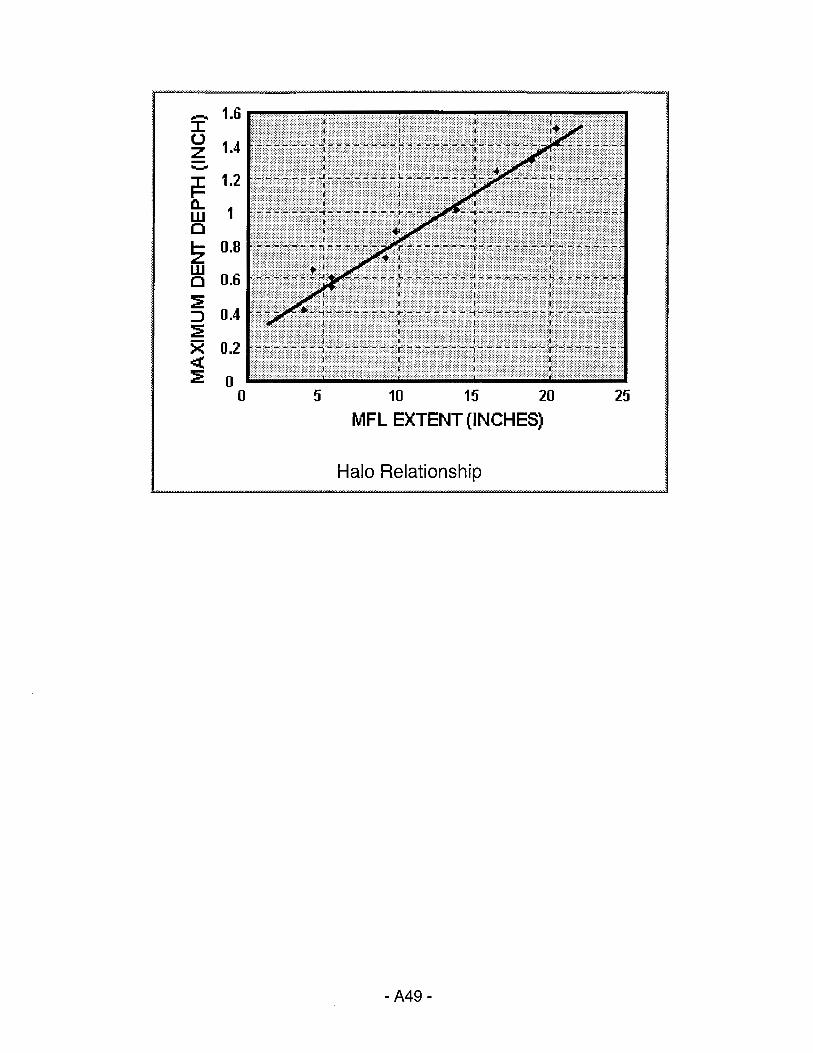
5 10 15 20 25 MFL EXTENT(INCHES)

Halo Relationship

-A49 -

Details on Recreating the Load-Deflection Curve and Predicting the Absorbed Energy

A method was developed to estimate the energy absorbed during the mechanical damage process. This method is based on a recreation of the load-deflection curve for the damage process. The method predicts the inward pipe displacement as a function of the radial indentor load as a function of the maximum indentor load, maximum dent depth, and residual dent depth.

The procedure for estimating the load deflection curve is as follows:

• Determine maximum vertical load from the amplitude of the decoupled signal

• Determine the maximum dent depth from the halo signal

• Measure the residual° dent depth using a caliper tool or other method

• Assume the initial slope of the load-displacement curve is the same as the unloading portion

• Based on the above, estimate the full shape of the load-deflection curve.

C c( 0 -I

DEFLECTION

Load Deflection Curve

-A50 -

Overview of Nonlinear Harmonic Method

Non-linear harmonics (NLH) refers to the use of an eddy current technique that is sensitive to the state of stress and plastic deformation in steel. Magnetic properties are affected by stress and deformation. As a result, harmonics of an input signal can be generated by the hysteretic characteristics of the magnetic properties of the pipe steel. In practice, the method begins with the application of a sinusoidal magnetic field at a fixed frequency to a material. A detector is used to sense odd-numbered harmonics of that frequency (typically the 3rd harmonic).

The following figure shows an excitation waveform as a solid line. The secondary voltage whose distortion represents a high third harmonic content is shown as a dashed line. This third harmonic can be detected using bandpass filtering or a lock-in amplifier. Because measurements can be accomplished using a relatively high excitation frequency, the method should lend itself to rapid scanning, and thus could be readily implemented on an inspection pig.

NLH Waveforms

-::J C.

8D51-'----hf--.l......,;.;;.~~ G) > i O ~~~~~--'-'r-,-

Nonlinear Harmonic Waveform

For more information on the effects of stress on nonlinear harmonic response, refer to Effects of Stress on the Harmonic Content of Magnetic Induction in Ferromagnetic Material

-A51 -

Details on Nonlinear Harmonics Measurements

NLH Measurement Program

The use of nonlinear harmonic technology for detecting and measuring stresses around a mechanical damage defect was evaluated in this program. The block diagram given below shows the system connections and instrumentation used for the nonlinear harmonic system. In Task 1, fundamental data were collected to demonstrate and quantify the sensitivity of nonlinear harmonics to applied stress and plastic deformation.

PIPE WALL

Nonlinear harmonic schematic

Using dog-bone and cruciform samples, small nonlinear harmonic probes were used to collect third-harmonic data as the samples were loaded both within and beyond the elastic range. The magnetic permeability of steel changes with applied stress and plastic deformation, and previous work also indicated that the nonlinear harmonic output changes with changes in magnetic permeability. It follows then, that nonlinear harmonic output should be an indicator of applied stress and plastic deformation. The laboratory experiments demonstrated that capability.

Following the initial laboratory experiments, several test specimens were fabricated with different types and severities of mechanical damage. The specimens were scanned with nonlinear harmonic probes oriented with the magnetic field in orthogonal directions. Amplitude and phase of the fundamental and third harmonic were collected and were used to generate line plots and color surface maps. These plots showed that nonlinear harmonic could be used to detect the stressed area around a mechanical damage defect.

Parameters that were varied included probe size, excitation frequency and probe orientation. There was also an initial evaluation of probe lift-off effects. The following figure shows a typical two-dimensional response to an undisturbed plate and a plate that has experienced plastic deformation. The figure on the left shows the initial nonlinear harmonic response, and the figure on the right shows the response after

-A52-

plastic strain has been applied. The change in signal is an indicator of the amount of strain that has accumulated.

Results to date show that it may be possible to use nonlinear harmonics to detect the stressed area around a mechanical damage defect. Additional parameters that are being studied include probe size, excitation frequency and probe orientation. There is also an evaluation of probe lift-off effects. This work is continuing, and conclusions will be drawn later in the program.

0.9

0.7

0ti

0.3

400< hdenl ,niso 3x3

■ 0.7-0.Q

lil0ti-0.7 I0.3-0ti

□ 0.1-0.3

□ -0.1-0.1

■ -0.3--0.1

S9 lil-0.5--0.3

09

07

05

03

0.1

-0.1

Undimnbed miso 3x3

Nonlinear harmonic plots

sg

■ 07-0.Q

805-0.7

■ 03-0.5

□ 0.1-0.3

□ -0.1-0.1

■ -03--0.1

llll-05--0.3

For more information on nonlinear harmonic measurements, refer to Nondestructive Measurement of Stress in Ferromagnetic Steels Using Harmonic Analysis of Induced Voltage and Application of the Nonlinear Harmonic Method to Stress Measurement in Steel.

-A53 -

Introduction to Neural Networks[Haykin99J

A neural network is an analysis method that uses a large number of relatively simple calculations to make a prediction. For example, a neural network can be designed to predict the shape of a corrosion defect or classify an indication based on information contained in the MFL signal. Although the calculations are simple, the large number of computations performed in concert allows neural networks to perform fairly sophisticated tasks.

The following figure is a graphical representation of the structure of a neural network. In the following figure, the input to a node (a connecting point) is shown by lines from the left and the output is shown by lines to the right. Each line represents a calculation, such as multiplying an input value by a constant. Each input parameter (e.g., signal amplitude, length, etc.) is multiplied by a (different) constant and used as input to the nodes. The action taken on the input is termed weighting or synaptic weighting.

Neural network concept

OUTPUT LAYER

A nonlinear function of the sum of the inputs to a node is calculated at the node. The function that is applied at the node to the sum is called the nodal function. Each nodal function has a set of parameters that further define it. The nodal functions are the

-A54 -

building blocks used for fitting the neural network's output to the training data. Nonlinear basis functions allow nonlinear fits to the data, which are needed for more complicated problems.

Sigmoid basis function

In a sense, each nodal function has a shape associated with it (for example, the shape of a logarithmic curve), and the output is made by summing various combinations of these shapes. For simple neural networks, such as those that make binary or yes/no decisions, sigmoidal or arctangent functions work best. For more complicated problems, such as predicting the shape of corrosion, certain functions are better suited than others in representing the intended output.

Gaussian basis function

In work done to date, several types of basis functions have been considered. In the multilevel perceptrons, a sigmoid function was used. The sigmoid function is a gradual step, from zero to one, as its input varies from negative to positive. It works best for binary decisions, such as whether a defect signal is from mechanical damage (output equals one) or not (output equals zero). The network can be trained to identify mechanical damage if the output is larger or smaller than some value.

For the more complicated problem of predicting defect geometry, radial basis functions were employed. Several radial basis functions were considered including Gaussian (an inverted bell shape), logarithmic (values ranging from negative infinity to positive infinity), and a multiquadric (values ranges from a finite number to infinity).

Typically, radial basis functions are centered about some point (a fixed value of an input parameter) and they vary with the "distance" or difference from that point. Radial basis functions provide a better ability to simulate the shapes of corrosion defects. They are

-ASS -

considered good approximators near the training data but are less accurate away from the training data.

In addition, a third set of basis functions, called wavelet functions, is being investigated. Wavelet functions are similar to radial basis functions. However they offer better approximation properties both locally and globally.

For more information on neural networks, refer to An Introduction to Computing with Neural Nets, Neural Networks: A Comprehensive Foundation, and Multivariate Functional Interpolation and Adaptive Networks.

-A56-

Overview of Training for Perceptron Neural NetworksrHaykin991

Determining the unknown parameters in a neural network is called training. Training is analogous to fitting a nonlinear curve through several points ~ there are many curves that pass through the same set of points. The key is to determine a set of parameters that reasonably matches the data and that can be extrapolated or interpolated to other sets of data. Forcing the fit to exactly match the data is possible, but usually produces poor results - errors can be introduced when the neural network attempts to predict random noise. When this happens, a neural network is said to be over-fitted. This is possible when the amount of training data is limited and is to be avoided.

The process of learning the values of the unknown parameters is at the heart of neural networks. The choice of the training method is important. Different methods have been developed (or are being developed in this program) with the goal of efficiently learning the parameters and producing a network that works well over a wide range of input conditions.

Training Example

Understanding the learning process of a neural network may not be intuitive. While different techniques are used, the method outlined below is fairly typical for multilayer perceptrons. The procedures for training radial basis function and wavelet networks are different.

Typically, at the start of training, random values are assigned to the unknown parameters. Hence, at this stage, the neural network will produce SOME ARBITRARY output. One set of input data is used, and the calculated output is compared to the desired output. As expected, they will differ. Next, the derivative of the output is taken with respect to each unknown parameter - that is, calculations are made to determine the gradient of the error function (how the output will change as each parameter changes independently).

Based on the gradients, a change is calculated for each parameter. Then, the changes are applied and the process is repeated with the next set of input data. If the problem were linear, one set of changes might produce a network that matches the data exactly. Usually, though, a change in one parameter affects all other calculations, and so, the network's output does not match the data. The process is repeated, and it is continued iteratively, until the remaining error falls below some arbitrary threshold. This process is known as learning.

The process of determining the derivatives and using them in the manner described above is called backward propagation. The term backward propagation is used to suggest that the errors are corrected back through the network using the derivatives or gradient of the error function.

Training the radial basis function networks and the wavelet networks are far more straightforward and do not involve the use of iterative procedures. The training

-A57-

procedure typically involves the inversion of a data matrix and is consequently easy to implement.

Graphical Representation of Classification Network

Input Ncdes

Hidden Ncde

X 1----► ·~-'--------:;./-4-:JIII.._

./ / ,-

/ ./

I / ;,,

/' ,I ·,·

:/ /

Output Ncde

1 0

0. : 1 J I

0000 .. ~. ~

0 -I Cl ·"'ffi

1u I :E

~--

Mechanical Damage

Multilevel perceptron structure

-A58-

Additional Details on Defect CharacterizationCHwan997.Hwan995J

Both radial basis and wavelet functions were used to perform three-dimensional defect characterization from the MFL signals. These networks were used to predict the shape of the defect (either corrosion or mechanical damage) using input parameters taken from the MFL signals. Typically, the MFL signal was transformed, for example, by converting the signal to its equivalent components in the frequency domain, after which 6 to 10 features from the transformed signal were chosen as input.

The radial basis function networks were developed under an earlier project for GRI. The wavelet network architecture is similar to that of the radial basis network, however, it uses wavelets for functional approximation. Wavelets can be expressed using

C C llr where "' and \Y' are known as the "centers" of the wavelet network, <)> and 'I' denote scaling wavelet functions, and ck and dk specify wavelet transform coefficients. The use of wavelets as basis functions provides a simplified training procedure and a trade-off between computational complexity and prediction accuracy in defect characterization.

A Gaussian radial basis function was used for scaling, and the Mexican hat wavelet, which is related to the second derivative of a Gaussian, was used as the wavelet function. The basis function width (one of the parameters describing the function) at the finest resolution was chosen in order to cover the full range of input parameters. The unknown weights were calculated using a matrix inversion technique.

-A59 -

Additional Details on the Prediction of Two-Dimensional Stress Fieldsnvanov9s1

Test Measurements

Two-dimensional stress fields were studied using defects installed on 4-inch by 1 /4-inch by 16-inch 1018 cold-finished flat steel plates. Two defects were placed on each plate to avoid the blooming effect of MFL signals for defects that are very near each other.

Two basic methods were used to prepare the defects. Simulated gouges were made by pressing a steel ball-bearing on the steel plate with a hydraulic pressure machine. Two different sized ball-bearings and ten pressure levels of the hydraulic pressure machine were used for a total of twenty gouge defects. A set of twenty corresponding metal loss defects was made by drilling out material from the plate.

The steel plates were magnetized with a custom magnetizer. The three components of the MFL signal from the defect were recorded with a Gauss meter for varying magnetization levels from about 1,300 Alm to 34,000 Alm. The specimens were magnetized to saturation, and the magnetizer was removed in order to measure the residual field signals.

Data were recorded for all defects for the active leakage field at saturation and the corresponding residual leakage field signals. Results showed nearly identical MFL signatures from the gouges and the metal loss at saturation. However, a large difference in the residual field signals was observed. A very small residual leakage field signal was recorded for the metal loss defects, while the leakage field was larger for the gouge defects.

-:naidt~I s:reB; I cc-npne~:; =-E -nee~! :i 1)1 ~. . . .,,..,...,..,...........,. 15

0

1./'..

1

.,i

Residual stress distribution

-A60-

Finite-Element Modelingnvanov971

Finite element modeling involved a structural analysis of the specimen in order to obtain the distribution of stresses from known loading conditions. An active "stress profile" was defined as the aggregate stress around the defect. The stress profiles and corresponding residual MFL signals were used as training data for the stress characterization algorithm. ~Finite Element Modeling of Defect Installation Process.

Mapping from the MFL signal to the stress profile was accomplished using a radial basis function network. The input to the network was taken from the residual MFL signal. In order to determine the optimal network configuration (i.e., to find the synaptic weights), both the training data and the support of the radial basis functions were varied (the support is one of the parameters that defines the functions).

The network was tested with MFL signals that were not part of the training set and the predicted stress profiles were compared with those generated by the mechanical damage finite element model. Typical results are shown below. The agreement between the predicted and desired profiles indicates that this method shows considerable promise.

Residual S ip,.al: 5/8" Ball O.,~ -~------~---,

-O.t) 10 2J 30 40 3J 60 'ill 80 Position

,....... O.c Residual S igral: 518" Ball

ij O.l /~ ~ / \_ 55klbs "-'0.4 ... ,\, lo.~ ~ 0 // \ i , \ ~-0., __ / \.

-0.l - ..._'--.----

-O., J 10 20 30 40 50 60 'ill 00

Position

1.5

Stress Profile: 518" Ball

Position

, I\ S tress Profile: 5/8 " Ball

10 20 Position

30 40

Two-dimensional stress distributions

-A61 -

3)

3)

Finite-Element Modeling of Defect Installation Process

The defect installation process was modeled by applying pressure on a small spherical pit on the top surface of a steel plate. The elastic behavior of steel was represented with a Young's modulus of 30x106 psi, a Poisson's ratio of 0.3 and specific density of 0.283 lb/in3

. The model was meshed with tetrahedral elements and care was taken that the element side length ratio did not exceed 1 :2. The nodes on the back of the plate were restrained (all degrees of freedom equal to zero) to avoid the change of geometry.

The load was perpendicular to the outer surface; therefore, the largest strains and stresses appear normal to the pipe surface. The external magnetization is along the pipe axis and is perpendicular to the largest component of the stress vector. The effect of compression was modeled by increasing the permeability, and similarly areas under tension were modeled by lowering their permeability values.

o.s •• ,, 0 -----------''!

-0.5

1 -1

i-1.5 v.o

-2

-2.5

-3

1

0.1 0.2

~, I , ___________ _

' 1

' I

1 , 1 I

' I I

' ' ' ' I I

' I

' ' ' ,,. - - - -.!

0.3 0.4 Distance

0.5 0.6 0.7

Stress distribution and stress profile for a 10 ksi, gouge

The results of elastic, static structural analysis for a load of 10 ksi are shown above. The top figure represents the distribution of the stress perpendicular to the top surface of the specimen, while the bottom figure shows the one-dimensional "stress profile" corresponding to that stress distribution. The elements directly under the pit are under compression, while the nodes on the edge of the pit experience tension. This is reflected in the "stress profile" as positive peaks above the edges and a negative peak under the pit.

-A62-

Details on Hysteretic Property Measurements11vanov991

Hysteretic parameters were measured using a Magniscope, an instrument designed and used in the Metals Development Lab at Iowa State University. This instrument allows "local" measurement of the B-H characteristics for ferromagnetic materials. The B-H curve is measured by magnetizing a small volume of the sample, using a yoke. The field intensity is measured, with a Hall probe located in the middle of the yoke. The probe is oriented to pick up the horizontal component of the field. The flux density is measured using a coil wound on the yoke. Parameters such as coercivity, remanence, and hysteresis loss are estimated from the B-H curve. The depth of measurement is roughly equivalent to half the distance between the poles of the yoke. A half-inch probe was used; the penetration depth was, therefore, approximately 0.25 inch.

Measurements were made on the surface opposite the defect. The scanning area was 3 by 3 inches, divided into a 12 by 12 grid, with the defect located in the middle of the scanned area. The measurement procedure included demagnetization, registration of a single hysteresis loop, and demagnetization again. Care was taken so that the orientation of the magnetic field remained constant. Measurements were taken with the field oriented in two perpendicular directions. Measurements were also made on a circular grid with eight divisions along the circumference and six divisions along the radius, resulting in 48 measurement locations. The magnetization field for circular measurement was radially oriented. This was done in order to maintain the symmetry of the residual stress field.

The resulting sets of data were processed and are shown below. The data were compared with the stress distribution patterns obtained from the structural finite-element model discussed earlier. For example, the scan shown in the first figure represents the distribution of coercivity (He) around a defect corresponding to a 30 kip load. The second figure shows the calculated residual stresses for the same defect.

The small variation of coercivity around the metal-loss defect in the first figure is a result of measurement and instrumentation error and does not indicate a variation of the coercivity of the material. No variation should be expected because the area is free of stress. The pattern around the pressed-in gouge exhibits a very large variation, on the order of 25 percent. This variation represents the residual stress in the sample due to the mechanical damage. The third and fourth figures show the distribution of remanence and hysteresis loss around the same defect. Similar results are observed.

The results suggest that the residual stress can be linked to magnetic parameters, such as coercivity, remanence, and hysteresis loss. All of the circular scans showed patterns of the shape similar to the expected stress distribution in the test samples. The sensitivity of a parameter to residual stress can be estimated from the relative change in the observed pattern. Remanence is more sensitive than coercivity, but hysteresis loss was most sensitive.

-A63-

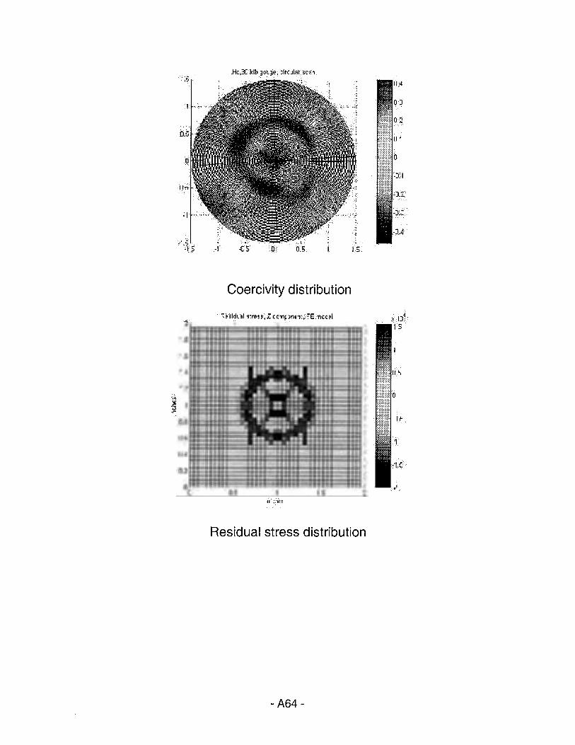
Coercivity distribution

Residual stress distribution

-A64-

Remanence distribution

Hysteresis loss distribution

-A65 -

Background on Stress Corrosion Cracking

Stress-corrosion cracking (SCC) results from the combined action of stress, a cracking (electrochemical) environment, and temperature to cause cracks to initiate and grow in a susceptible line-pipe steel. Individual cracks are generally oriented perpendicular to the maximum stress and parallel to the pipe axis. Groups of cracks usually occur in what is known as a "colony." In extreme cases, these colonies may be several feet long and extend nearly around the circumference.

SCC colonies are considered sparse if the cracks are far apart in the circumferential direction and dense if the cracks are circumferentially close together. Individual cracks can range from shallow to deep. Many cracks in the middle of dense colonies have a depth less than ten percent of the wall thickness. In sparse colonies and in some dense colonies, the cracks can grow in a stable manner until they reach nearly through the wall. These deeper cracks are of primary concern in inspections to evaluate pipeline integrity.

Stress Corrosion Cracking

As nearby cracks grow, individual cracks can coalescence or join to form a single, larger crack. If the coalesced crack is long enough, it can rupture. The consequences of a rupture are usually more severe than those of a leak. As a result, long deep cracks, and deep cracks that are close enough to coalesce into a crack that is long enough to rupture, are of primary concern when inspecting pipeline.

Two forms of SCC have been encountered: high pH and low pH. The surfaces of most low and high-pH stress-corrosion cracks are not smooth but irregular. High-pH stress­corrosion cracks are typically intergranular (with a cracking path along the grain boundaries of the material), with essentially little or no separation or opening between the crack faces. Low-pH cracks are often transgranular, where the fracture surfaces are smoother than intergranular fracture surfaces, but they are not as smooth as fatigue cracks. Also, both forms of cracking can branch as cracks grow through the wall thickness.

-A66-

Additional Impact of Cracks on Inspection Requirements

The severity or criticality of a set of stress-corrosion cracks is most strongly a function of the length, depth, and spacing between individual cracks. Crack length and depth, along with stress level and pipe toughness, determine whether an individual crack will fracture or fail unstably. Spacing between cracks determines whether one or more cracks will coalesce before or during a failure. The nucleation and growth of stress-corrosion cracks are becoming better understood, and models for predicting crack criticality are in development. However, detailed predictions are not yet feasible. The following discussion focuses on the likelihood of near-term failure as a primary criterion for determining which cracks should be found.

Years of pipeline operating experience have demonstrated that small imperfections (for example, small regions of corrosion metal loss) cause only a small reduction in failure pressure. If the imperfections do not grow, they do not significantly threaten the integrity or serviceability of a pipeline. Consequently, in developing guidelines for acceptable corrosion loss during the 1960s and 1970s, the pipeline industry defined a hydrotest to the specified minimum yield (or design) strength as a fundamental requirement for pipeline safety. An acceptable imperfection was defined as one that could pass such a hydrotest. A defect was taken as one that would not survive a hydrotest of 100 percent of the pipe's yield stress.

In recent work, Battelle developed a comprehensive failure criterion for individual stress­corrosion cracks in a program sponsored by the Pipeline Research Committee. This criterion is more accurate than and represents a significant improvement over corrosion flaw severity criteria used by the pipeline industry.

Stress-corrosion cracks cannot be considered independently, though, because their ultimate failure may involve coalescence of several cracks. If two (or more) cracks coalesce, the resulting crack length increases. As a result, the coalescence of several cracks that could each survive a high-pressure hydrotest could result in a single crack that would be on the verge of failure at typical operating pressure. As a result, basing inspection requirements on failure at high pressure alone, without considering the likelihood of coalescence, could lead to nonconservative results if nearby cracks coalesce. Accounting for the likelihood of coalescence increases the emphasis on shorter, deep cracks in setting inspection requirements.

-A67-

Details on the sue Systems

In the 1980s and early 1990s, Southwest Research Institute (SwRI) developed two inspection techniques to overcome problems associated with sizing near-surface axial cracks from the outside surface of a pipe. The SwRI techniques are referred to by the acronym SLIC, which stands for simultaneous use of shear and longitudinal waves to inspect and characterize flaws.

The SLIC-30 module is designed to enhance the ability of an ultrasonic examiner to estimate small crack depths. Two transducers are used, one to transmit a wave and one to receive. The first transmits a nearly perpendicular (70 degree) longitudinal (compression) beam that is directed at the crack face. This beam generates a set of longitudinal waves that are nearly parallel to the crack from both the surface and the crack tip. A second, low-beam (10 degree) transducer measures these secondary pulses.

The SLIC-50 system is designed to overcome shoe noise and surface reverberation that can mask the weak diffracted signals from the bottom of a shallow crack. Unlike the SLIC-30 system, the SLIC-50 system receives both longitudinal and shear waves. This feature allows the system to measure crack depth regardless of the separation between the transducer and the crack.

The SLIC-50 system operates by transmitting an interrogating wave, and then sensing a pair of associated diffracted signals (a doublet, for short) from the crack tips in the through-wall direction. A unique feature of the SLIC-50 system is that the distance between the doublet signals is practically independent of the position of the sensor.

-A68 -

General Theory of Velocity-Induced Remote Fields

Conventional pipeline inspection tools generate axially oriented magnetic fields, which are sensitive to the presence of circumferential cracks. The inspection tool is insensitive to SCC, though, because they are oriented largely in the axial direction. A possible alternative is to utilize the fields associated with the circumferential currents generated in the pipe wall by the movement of the magnetizer relative to the pipe wall.

The most general governing equation describing the physics underlying the motion of a pig in a pipe with a defect is:

1 - - aA - -Vx-VxA = Js - a-+ aVxVxA µ, at (1)

aA a-

Where the term at represents the defect-induced current density resulting from the time-varying magnetic field caused by the changing spatial relation between the defect

and magnetizer. In the case of a defect-free pipe, this term is zero. The term a V xv x A represents the currents induced by the velocity of the magnetizer relative to the pipe wall.

Since the motion of the tool inside the pipe is along the pipe axis, the motional electro­

magnetic force due to the V x B term is negligible between the poles of the magnet. However, at the poles, the radially oriented magnetic fields generate a significant amount of circumferentially directed currents in the pipe. The intersection of these motion-induced currents with axial cracks results in a perturbation of the current distribution.

The fields associated with the perturbation currents carry information related to the axial cracks. In general, the fields and resulting currents are large close to the magnetizer, making the measurement of small perturbation fields difficult. So, in this work, we considered the current perturbation in the remote field region of the magnetizer.

-A69 -

Details on Finite-Element Modeling of Velocity-Induced Remote Fields [Yang981

Modeling of the interaction between axial cracks and circumferential currents is a significant challenge in terms of computation time and memory requirements. The challenges arise due to nonlinearity of material properties, the size of the cracks relative to that of the magnetizer, and the time stepping involved in modeling velocity effects. The approach used here to surmount these difficulties was to decompose the overall task into three simpler subtasks that can be performed sequentially:

• Step 1: Calculate velocity induced currents 10 in a defect-free pipe wall due to axial motion of the magnetizer inside the pipe. (m1Step 1 Graphic)

• Step 2: Model an axial crack by applying a current -Ioli at the nodes i defining the

crack and compute total perturbation current Jp. (imStep 2 Graphic)

• Step 3: Use results obtained in Step 2 to solve for the perturbation fields that can then be measured with an induction coil. Details associated with each step are provided below. ( ioiStep 3 Graphic)

Step 1. Calculation of Velocity Induced Currents

In the first step, a defect-free pipe with a magnetizer moving at a fixed velocity is modeled. The velocity induced current in the defect free pipe wall is calculated using the Leisman-Frind method. The axial distribution of currents on (1) the inner surface, (2) middle of pipe wall, and (3) outer surface of the pipe wall show that in the vicinity of the magnetizer, the current decays from the inside to the outside diameter of the pipe. The motion of the magnetizer at a fixed velocity, therefore, results in a current distribution that varies with each time step. The current is used as the source term in step 2, which models a section of the pipe wall in the remote field region. lDetails of Step 1.

Step 2. Calculation of Perturbation Current by the Presence of a Crack

In step 2, a tight crack of zero volume is introduced in the remote field region of the pipe. The basic assumption in this step is linearity of constitutive relations in the remote field region. That is, the total current in the presence of a crack is the sum of the background current in the defect-free pipe and the perturbation current introduced by the crack. Using this approach and ignoring the defect induced current term in the equation, we apply Neumann boundary conditions at the nodes to determine the perturbation currents to a first approximation. fRDetails of Step 2.

Step 3. Calculation of Current Perturbation Fields

In the third step, the three-dimensional governing equation in terms of the vector magnetic potential is used to calculate the first approximation of the magnetic fields

-A70-

induced by the perturbation currents. This potential is then used to determine the defect-induced term that was ignored in the previous steps by iterating until convergence is obtained. The final solution is then used to calculate the associated flux density.

The motion of the tool is modeled by implementing steps 2 and 3 for each position of the defect relative to the inspection tool and the sensor coil. The induced voltage in sensor coil is then computed as a function of position. liDetails of Step 3.

Example

The inspection.11eometry used in the implementation of the finite-element model is shown below. lii&lExample of three-dimensional simulation of velocity-induced remote fields. This defect-free geometry is axisymmetric and, hence, a two-dimensional model was used in implementing step 1 to calculate the velocity-induced currents in each time step. In steps 2 and 3, the boxed section around the axial crack was modeled in three dimensions using the source currents obtained in step 1.

direction of tool motion (5 m/s)

◄ OD

Example geometry

The resulting defect signals were calculated in terms of the voltage induced in a single turn coil by the axial component of the perturbation fields. The voltage signal as a function of the depth is shown below. The peak signals occur at the crack edges.

- A71 -

X 10-6 2.5'~--~---~---~--~

..... 2 II z 1.5

u -5 -1.5 C: - -2

;

-5 D

Cm

\,

- 20% - - .. - <10% ----- 60%

. ' \, ,' '·./

5

80%

I

Induced voltage in a single turn coil for different defect depths

-A72 -

1 D

Graphics for Steps 1, 2, and 3

.. Governing Eq1rntion: 'v x t 'v x A = J, - cr 8 A + cr v x 'v x ~~ ,.L at ( Le ismann-Frind lVle thod)

" Output: Velocity induced CutTent Distribution in defect free pipe (JO)

cj Dirichlet B.C.

iri 0 OD Pi e\vall g

Re:mote region~

~ ID bru:shes

z magnet

.. CTOverning Equation: Vx .A-vx A= L-cr 0 A + crV x: Vx .. ~ ~ · at ·

( Leismann-Frind 1l1e thod)

w Output: Velocity induced Cuffent Distribution in defect free pipe (JO)

u Dirichlet B.C.

iri 0 OD Pi ewall g

Reinote region~

~ ID bru:shes

magnet z

~ G-Ove1·ning Equation: V X }II V X .~ = J, - a a A + a V X V X I . at ( Le ismann-Frind l'4i! thod)

* Output: Velocity induced Ctm-ent Distribution in defect free pipe (JO)

0 Dirichlet B. C.

~ Remote region~ z t::: OD Pi ewall § §

! ID bru!lles § ::i

z magnet td

Dirichlet B.C. 0

-A73-

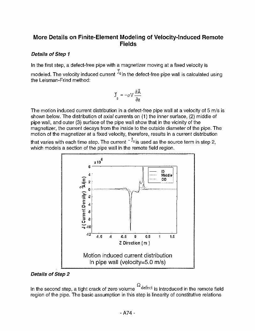
More Details on Finite-Element Modeling of Velocity-Induced Remote Fields

Details of Step 1

In the first step, a defect-free pipe with a magnetizer moving at a fixed velocity is

modeled. The velocity induced current 10 in the defect-free pipe wall is calculated using the Leisman-Frind method:

aA J =-aV-o az

The motion induced current distribution in a defect-free pipe wall at a velocity of 5 mis is shown below. The distribution of axial currents on (1) the inner surface, (2) middle of pipe wall, and outer (3) surface of the pipe wall show that in the vicinity of the magnetizer, the current decays from the inside to the outside diameter of the pipe. The motion of the magnetizer at a fixed velocity, therefore, results in a current distribution

that varies with each time step. The current - Jo is used as the source term in step 2, which models a section of the pipe wall in the remote field region.

Details of Step 2

6

4

&2 c--'fC

0 -~ 'in -2 C: (I) 4

0 ..... C: -6 e ,_ ::J -8 u ::;.10

-12

x10 6

-1.5 -1

ID Middle

·········· OD

.0.5 0 0.5 1.5

Z Direction ( m )

Motion induced current distribution in pipe wall (velocity=5.0 m/s)

Q In the second step, a tight crack of zero volume defect is introduced in the remote field region of the pipe. The basic assumption in this step is linearity of constitutive relations

-A74-

in the remote field region. That is, the total current Jin the presence of a crack is the

sum of the background current Jo in the defect-free pipe and the perturbation anomalous

current JP introduced by the crack:

- { -Jo J = p

unkno'W!l

in Qdmct

where Q~ct is the complement of QM!ct . The total current is given by:

Q On defect we have

Jp = -J0 = a(jw.A. + VV)

where V is the electric scalar potential.

Using this approach and ignoring defect induced currents, jwa.A., we apply Neumann boundary conditions at the defect nodes i:

Jo a.

l

The solution of the governing Laplace Equation V2V = Ogives to a first approximation,

the perturbation currents JP in the pipe wall section due to an axial crack.

Details of Step 3

In the third step, the three-dimensional governing equation in terms of the vector magnetic potential is used to calculate the first approximation of the magnetic fields induced by the perturbation currents. This potential is then used to determine the defect contribution to the current that was ignored in the previous step by iterating until convergence is obtained. The final solution is then used to calculate the associated flux density.

The governing equation for this step in terms of the vector magnetic potential is the three-dimensional equation

1 - -\7X-\7XA = Jp µ,

-A75 -

where Jp is the current distribution obtained in step 2. The solution of this equation is the first approximation of A . The solution is substituted in the earlier equation in the

term jwa.A. to correct the value of Io, and steps 2 and 3 are iterated until convergence is obtained. The final solution A is used for computing the associated flux density B=VxA

As an example, the axial component of the field (B2) obtained in step 3 is plotted below. Note that the figure corresponds to the axial field component at one position of the magnetizer relative to the crack.

-·-.., ...... I _,-

2 ---- '

0 -

-2 - - - - - ' ..,: ... - _, ... ... -4 ,. _,.,.,. - : _, ...... ~

E __ ...... --:---- J __ .,.,. ~ -6 - I .,. ,.._. I

~ ------r::.--~-----10 ., .,. ... - ....... ... .J...._, ...... ,- .,

-12 _____ :<:-· 40) ---~~:

- .,.. '"r· ... --- I --

1 ~-.,.,. ... 1 ......... - : .........

I -... t-- ... .,.,.I,.._ I-...._ I ""..,

I ...... I ...... I t ... ,.,_.., ~..,.., I ._ .._

I ', I '"..,I l .._ I ....... l'.,, I

._ L., I .._..,.., : ._ ..... ~

.., 'I.' I

... ... : ......... ~ -. l.,. "L., I...... :

- ... : ........ : ...... __ • .. ... J

--~ -~--- t- ..... : ------.... : ........... : ... -~ ... ~ ..... --~ ............ f', ...... :-----.:

.., ... --~,, :-- ... : .,.,. ......... :: -.._'.-!. ._i

_, ...... - ~: .... :.,. ... - .,. .................. : .. __ J'... .. _, .....

.,.,- ...... ; ... :, J:O

0 ...__ -

_, ..... - ..... 0

.Jl)

Z(mtf\) .4)) .Jl)

Pli(~

Axial component of magnetic field

The motion of the tool is modeled by implementing steps 2 and 3 for each position of the defect relative to the inspection tool and the sensor coil. This results in values <I> ; of the total flux linking the coil at each position. The induced voltage in sensor coil is then computed as a function of position j:

V. Nd#. 12 1=- -,1= ···n dt ' ' '

=-N(ct,i-ct,i-1)

where, Vi is the signal due to axial component of current perturbation fields and N is number of turns of coil.

-A76-

Example of Three-Dimensional Simulation of Velocity-Induced Remote Fields

The inspection geometry used in the implementation of the finite-element model is repeated below. The pipe wall was taken as 9 mm thick, and the magnetizer and the pick-up sensor moved at a fixed velocity of 5 meters per second. The sensor was taken as a single turn coil of dimension 2.45 cm x 6.25 cm, located in the remote field (30 cm behind the magnetizer) and 0.1 cm below the inner pipe wall. The plane of the coil was assumed to be perpendicular to the axis of pipe. The resulting defect signals were then calculated in terms of the voltage induced in a single turn coil by the axial component of the perturbation fields.

direction of tool motion (5 mis)

Example geometry

The voltage signal as a function of the depth of a crack whose length is 8 cm is shown below. The peaks occur at the crack edges.

-A77-

X 10-6 2.5.------~--~--~----,

..- 2 :!! 1.5 -~ 1 0 > I

:·,

I ' - 20% ........ ~0% ·····- 60% - - 80%

- 0 .5 .. - · -~-- \ g> 0 ~, ... ~,-:.-~------- -,_~ .., ~~=------ _, _ _. :~

....., ·• .••. • •• , '•-~ - I

~-0.5 \ --------

al -1 u -5 -1.5 C: - -2

-2 ~10 -5 0

Cm

.. / 5 10

Induced voltage in a single-turn coil for different defect depths

The peak-to-peak values plotted as a function of flaw depth show an exponential variation:

.... 5

4.5

.... :!!: 4 0

<UZ° .:!o 3.5 ro> >'a, 3

.:,,:: C)

~~ 2.5 a.c5 .s> 2 .:,,:: "C

~ ~ 1.5 D... ::I

]l1 0.5

-6 l 10

020 30 40 50 60 70 BO

Defect depth (%)

Peak-to-peak induced voltage in a single-turn coil as a function of defect depth

The signals obtained with various axial crack lengths are plotted below. The results show a monotonic increase in the peak value of the signal with defect length.

-A78-

10

9 -=:ll: 0 .-,: 8 G) :!:: .2 >o 7 tv -> G)

~E 6 G) -Q. 0

.E > 5 -"" -a tv G> G) ... 4

II.. -5 C

3+--~-~-~-------' 3 4 5 6 7 8

2 Defect length (cm)

Peak-to-peak induced voltage in a single-turn coil as a function of defect length (60% depth)

The signals shown in earlier were obtained when the coil axis was directly under the flaw. The signals obtained at other circumferential coil axis positions show a reduction in magnitude. The voltage signals at 0°, 7.9°, 15.8°, and 23.7° are plotted below. These signals show a reduction in the peak amplitude of the signal as the coil moves away from the crack.

X 10"6 2.5 r----~--~----.-----,

2

_ 15 II

z_ 1

- □ degrees

- - - - 7.9 degrees

--·---15.8 degrees -··-· 23.7 degrees

~0.5 ,,-,.,i ··-- ..

i O ><-' ~ ~-05 -0

~ -1 ::s :g_15

-2

-2 ~10

I -":-• :,/;,,.--~ ..... ___ _

-5 0 5

Axial Direction (Cm)

10

Induced voltage in a single-turn coil as a function of circumferential position

-A79 -

Overview of Remote-Field Eddy-Current Techniques

In prior work for the Pipeline Research Committee, the remote-field eddy-current technique was successfully used to detect a variety of defects and material conditions in large-diameter pipeline steels. Limitations of this technique were also identified. In this project, we investigated methods to address these limitations by improving the sensitivity of the technique and increasing the inspection speed.

Traditional remote-field eddy-current techniques use low-frequency exciters, which limits the maximum speed at which inspection equipment can travel. Typically, these speeds have been less than one mile per hour, which severely limits the potential uses on in-line inspection equipment. Detecting SCC depends on the strengths of the eddy currents, which in turn, depend on the electrical conductivity and magnetic permeability of the pipe material.

A schematic of the remote-field eddy-current technique is shown below. An exciter, which is sized to nearly the same diameter as the inside diameter of the pipe, is driven with a low-frequency sinusoidal current. A small magnetic field sensor is positioned some distance away. One portion of the magnetic field generated by the exciter travels down the inside of the pipe, with the field directly coupled to the sensor. A second portion of the alternating magnetic field propagates through the material of the pipe, inducing eddy currents as it goes. Once the magnetic field penetrates the outside wall of the pipe, it spreads along the surface of the pipe and re-enters the pipe, again inducing eddy currents to flow in the pipe material. This second path is referred to as the remote path.

Remote (far) Field Coupling

Direct Coupling

Exciter Coil

Remote-field eddy-current concept

The total magnetic field and eddy current flow at any point is the combination of directly coupled and remotely coupled fields. The key to remote-field eddy-current testing is to choose a sensor position where the remotely coupled field is large compared with a directly coupled field. This is possible because the directly coupled field decays at a faster rate.

Shown below is a semi-logarithmic plot of the decays of both the remote and direct field. Both decays are exponential and the decay constant for the direct field is nearly four

-ABO-

times as fast as the remote field. Also, the combined magnetic field is less than the direct field in the near field, and it is less than the remote field in the far field. This phenomenon is due to the fact that phase difference for the two paths is always greater than 90 degrees for distances greater than a coil diameter.

1.0e-1,----------------,

.J. 1.0e-2

~ 1.0e-3

~ 1.0e-4 0,:

~ 1.0e-5

~ 10e.S u.. 0 i!j 1.0e-7

E 10,.a 13 <( 1.0e-9 :ii

Direct Coupling -------- Remote Coupling - TotalFie1dDetec1ed

1.0e-10------,.-.....---,------,--.......-----,---.,..,

2

DISTANCE FROM EXCITOR COIL

[ Pipe Diameters)

Relative signal strengths

At a distance from the exciter coil that is greater than about three pipe diameters, the remote field is larger than the direct couple field, and it constitutes the bulk of the total field. By placing a sensitive detector in this region, perturbations in the remote field as a result of axial cracks can be detected.

-A81 -

Details on Remote-Field Eddy-Current Experiments

Remote-field eddy-current techniques were investigated using the MFL test bed vehicle and various exciter coils and sensors. A sinusoidal current flowing in an exciter coil was used to induce currents in the pipe at various background magnetization levels. The test bed vehicle supplied the background fields needed to reduce the permeability of the pipeline steel.

Three critical experiments were performed to evaluate the improvements made to remote-field eddy-current results using magnetic saturation. They were used to

• Determine the placement of remote-field eddy-current exciter coil

• Detect stress corrosion cracks using exciter coil saturation

• Demonstrate noise reduction with magnetic saturation.

The results show that the relative permeability µr of the pipe can be reduced from 98 to 15 using magnetic saturation. This means the signal amplitude at the receiver should be nearly 6.5 times ( > 98 / 15) greater with saturation than without.

Signal amplitude is proportional to the inverse of excitation frequency. The excitation frequency, in turn, limits the maximum inspection velocity: the higher the frequency, the higher the possible inspection speeds. By decreasing the relative permeability by a factor of 6.5, a 20-hertz signal through unsaturated pipe and 130-hertz signal through saturated pipe have the same signal level at the receiver. Hence, magnetic saturation could be used to help overcome implementation difficulties related to maximum inspection speed or signal amplitude.

The following figure shows a typical signal for a crack acquired at an excitation frequency of 100 Hertz. For this test, one sensor was rotated past the crack in the circumferential direction. Additional metal, in this case a 3/4-inch steel nut, was used to ensure the remote-field signal was being measured. As seen in the figure, the nut was placed next to the crack and subsequently on the crack. Placing the nut on the crack reduced the amplitude of the crack signal.

-A82 -

rn 22 rn ::I Ol

(!)

.. 20 "O ::I ~

0. E 18 <

16

,-~. - r, ~~;: sec .

"'~:'\ //'-_Y'\~',:::_ Metal Loss \ , f· I , C

. ,, j /

orros1on \ \ ! I -· ·

\ \I f \__ Nutat4" \ i

/ : / \ I \ /'

~ Stress Corrosion Crack

14 0 5 10 15 20 25

Circumferential Distance (inches)

Remote-field eddy-current results

The signal levels at 100 Hertz were adequate for defect detection, but additional signal amplitude is always helpful. Since saturation at the exciter was useful, we expected that saturation at both the exciter and the receiver would provide even better signal levels. We attempted to verify this expectation as follows. The TBV magnetizer was used to provide magnetization at the exciter coil, and local magnetization was performed at the receiver coil by placing magnets on the outside of the pipe. Saturation at the exciter and receiver provided increased signal levels over the exciter saturation only, but the saturating field at the receiver was not uniform, and the drift in bias signal level masked the defect signals. Hence, the tests were not successful. Additional work is needed here.

An interesting result was observed when the receiver magnets were removed from the outside of the pipe, and the experiment was repeated with exciter saturation only. The noise levels were greatly increased in the regions where the magnets were placed and then removed. We hypothesize that the source of the noise was a randomization of the magnetic domains caused by the application and removal of the magnets. Consequently, aligning the magnetic domains by remagnetizing could reduce the background noise levels. To prove the potential this concept, the test bed vehicle was pulled through the test sample to realign the magnetic domains, and then the exciter saturation experiment was repeated. The signal and noise levels matched previous results, demonstrating the increase in noise due to randomized magnetic domains.

While the experiments with saturation at both the exciter and receiver coils were not successful because of equipment limitations, this technique should further increase the excitation frequency enabling. Also, the remote-field eddy-current technique with magnetic saturation has potential for detecting other defects in pipelines in addition to cracks.

-A83-