Embed Size (px)
Citation preview

What drives Q and investment fluctuations?
Ilan Cooper Paulo Maio Andreea Mitrache1
This version: September 2017
1Cooper, [email protected], Department of Finance, Norwegian Business School (BI); Maio,[email protected], Department of Finance and Statistics, Hanken School of Economics; Mi-trache, [email protected], Department of Economics and Finance, Toulouse BusinessSchool.

Abstract
A dynamic present value relation implies that variations in the ratio of the marginal prof-
itability of capital to marginal Q are driven by shocks to the expected growth of the marginal
profitability of capital or discount rate shocks, or both. We find that this ratio predicts future
marginal profitability of capital growth at horizons of up to 20 years, but not investment
returns. Thus, in contrast to stock prices, the primary source of fluctuations in marginal Q as
well as of aggregate investment is expected profit growth shocks, whereas the role of discount
rate shocks is negligible. The results indicate that managers’ real investment decisions are
strongly related to economic fundamentals.
Keywords: Asset pricing, Tobin’s q, Present-value model, Investment returns, Long-
horizon regressions, VAR implied predictability
JEL classification: G10; G12

1 Introduction
The neoclassical Q-theory of investment implies that under linearly homogenous tech-
nologies the marginal value of capital, termed marginal Q (Tobin (1969)), is a sufficient
statistic to describe investment behavior (Hayashi (1982)). Marginal Q is the present value
of all future marginal profitability entailed by installing an additional unit of capital. Thus,
similar to stock prices, variations in marginal Q are driven by shocks to expected cash flows
as well as by discount rate shocks.
In this paper we explore the sources of variation in marginal Q and aggregate investment.
This is important for at least two reasons. First, aggregate investment is highly procyclical
and one of the main drivers of the business cycle. Thus, uncovering its sources of variation
will enhance our understanding of the business cycle.
Second, a large literature explores the sources of variation in stock prices (see Campbell
and Shiller (1988), Fama and French (1988), Cochrane (2011)). While stock prices are
determined by investors in the stock market, it is company managers who ultimately assess
the marginal value of capital and base investment decisions on their assessment. Stock market
investors are susceptible to the influence of investor sentiment and several other behavioral
biases. Managers, however, may be less susceptible to these biases because they have more
information about their firms.1 Thus, fluctuations in marginal Q and investment could
originate from different sources than stock prices. For example, the finding that discount
rate shocks are the sole determinant of variation in the aggregate dividend yield (Cochrane
(2008)) are consistent with time-variation of risk or risk aversion but also with waves of
investor sentiment leading to mispricing of stocks. It might be, therefore, reassuring if the
source of fluctuations in marginal Q and investment is different.
To identify marginal Q, we refrain from using observable measures of Q (such as the
market-to-book ratio) that could be contaminated with measurement errors (see Erickson
1For example, Hribar and Quinn (2013) find that managers’ trades are negatively related to investorsentiment, and especially so with stocks that are difficult to value.
1

and Whited (2000)). Instead, we employ the Euler equation from the firm’s optimization
that equates the marginal value of capital to the marginal cost of investment. Assuming
a (standard) functional form of the adjustment cost of investment (as in Liu, Whited, and
Zhang (2009)) enables us to identify the marginal cost of investment and thereby the marginal
value of capital, namely marginal Q. We note that the model-implied marginal Q is a function
of investment. Our approach is therefore a supply approach to identifying Q, and is similar to
that of Belo, Xue, and Zhang (2013) who use the supply side, that is, the firm’s optimization
conditions, to identify Q.
We use generalized method of moments (GMM) to match the mean of levered investment
returns to the mean of stock returns (as in Liu, Whited, and Zhang (2009)) and to match
observed marginal Q in the data to model-implied marginal Q (as in Belo, Xue, and Zhang
(2013)). We conduct the GMM estimation at the aggregate level for all firms on Compustat
for both value-weighted and equal-weighted aggregate portfolios.2
We derive a dynamic present value relation, according to which fluctuations of the log
ratio of the marginal profitability of capital to marginal Q (which we intermittently refer
to as mq) emanate from shocks to the expected growth rate of the marginal profitability
of capital, or discount rate shocks, that is, shocks to expected investment returns, or both.
This present value relation is reminiscent of the Campbell and Shiller (1988) decomposition,
where mq plays the role of the log dividend-to-price ratio.
In our model specification, marginal Q is a linear function of the investment-to-capital
ratio. One could derive a present value relation for marginal Q as well (see Lettau and Lud-
vigson (2002)). Such a present value relation links marginal Q to future investment returns
and to future marginal profitability and not future growth rates of marginal profitability.
There are two advantages of a variance decomposition of the marginal profitability of capital
to marginal Q over a variance decomposition of marginal Q itself. First, examining the pre-
dictability growth rates of marginal profitability emphasizes high frequency aspects of the
2As a robustness check, we also estimate the parameters using decile portfolios sorted on Q.
2

data that the empirical models may be better able to capture in the presence of slow mov-
ing and unobserved changes in technology (see Barro (1990), Morck, Shleifer, and Vishny
(1990), Cochrane (1991), and Chen, Da, and Larrain (2016) for related discussions). Sec-
ond, examining the predictability of marginal profitability growth and investment returns
using mq allows a direct analogy to the vast literature on the variance decomposition of the
dividend-to-price ratio (Campbell and Shiller (1988), Fama and French (1988), Cochrane
(2008, 2011), among many others).
We estimate weighted long-horizon regressions (as in Cochrane (2008, 2011) and Maio
and Santa-Clara (2015)) as well as conduct a variance decomposition for mq based on a first-
order VAR (following Cochrane (2008)). We find that the ratio of the marginal profitability
of capital to marginal Q is a strong predictor of the growth rate of the marginal profitability
of capital at horizons between one year and twenty years. mq does not have any predictive
power for investment returns though. Noticing that marginal Q is three times more volatile
than marginal profit, much of the variation in mq stems from variations in the log marginal
Q. We conclude that the main source of fluctuations in both marginal Q and aggregate
investment are shocks to expected growth of the marginal profitability of capital.
Abel and Blanchard (1986) calculate an approximation for the two components of marginal
Q, namely expected returns and expected marginal profitability. They find that most of the
variability in marginal Q is generated by variability in the cost of capital, whereas the
marginal profit component of marginal Q is more closely related to aggregate investment.
Abel and Blanchard (1986) argue that a possible explanation to their finding regarding a
weak relation between aggregate investment and discount rates is that they have been less
successful in constructing the cost of capital component of marginal Q than the marginal
profitability component.
Cochrane (1991) finds that the aggregate investment to capital ratio predicts the future
stock market return as well as future investment returns. Cochrane’s result suggests that
the cost of capital is a driver of investment, which seems to be somewhat at odds with the
3

conclusion reached by Abel and Blanchard (1986). Our methodology does not require the
construction of any approximation, although it does require parameter estimation. Thus,
we provide an independent test of the drivers of marginal Q and investment. Our results
regarding the link between expected marginal profitability shocks and investment are overall
consistent with those of Abel and Blanchard (1986). Given that we take the supply approach
to valuation (as in Belo, Xue, and Zhang (2013)), that is, we identify marginal Q using
investment, our results are very different from those of Abel and Blanchard (1986) regarding
the sources of fluctuations in marginal Q. That is, we find that shocks to the marginal
profitability of capital are the sole drivers of variation in marginal Q.
Lettau and Ludvigson (2002) show theoretically and confirm empirically that predic-
tive variables for excess stock returns over long horizons can also predict future investment
growth. Chen, Da, and Larrain (2016) use accounting identities to decompose unexpected
investment growth to surprises to current cash flow growth and stock returns, shocks to ex-
pected cash flow growth, and discount rate shocks. They use a VAR to extract unexpected
components, and find that current cash flow shocks account for the bulk of unexpected
aggregate investment growth. Chen, Da, and Larrain (2016) also find that discount rate
shocks are unimportant for unexpected aggregate investment growth. They find a negative
covariance between unexpected investment and expected cash flow shocks. This finding is
very different from our finding that variations in aggregate investment predict positively the
future marginal profitability of capital. Moreover, Chen, Da, and Larrain’s (2016) result
crucially depend on their VAR specification.
Our work also relates to the growing literature that studies stock return predictability
by financial ratios in association with present-value relations. This literature emphasizes
the benefits of analyzing jointly the predictability of future stock returns and cash flows by
computing variance decompositions for the financial ratios. Most of the work is concentrated
on the predictability from the dividend yield (e.g., Cochrane (1992, 2008, 2011), Lettau and
Van Nieuwerburgh (2008), Chen (2009), Binsbergen and Koijen (2010), Engsted, Pedersen,
4

and Tanggaard (2012), Asimakopoulos et al. (2014), Rangvid, Schmeling, and Schrimpf
(2014), Maio and Santa-Clara (2015)). On the other hand, several studies compute variance
decompositions for other financial ratios like the earnings yield, book-to-market ratio, or net
payout yield (e.g., Cohen, Polk, and Vuolteenaho (2003), Larrain and Yogo (2008), Chen,
Da, and Priestley (2012), Maio (2013)). Koijen and Van Nieuwerburgh (2011) provide a
survey.
The rest of the paper is organized as follows. In section 2 we present a model of a firm’s
optimal investment decisions. Section 3 describes the data and the econometric methodology
for estimating the production and adjustment costs parameters. We derive the present value
relation linking mq to future cash flows and discount rates in Section 4. Section 5 presents
the benchmark empirical results when using weighted long horizon regressions, while Section
6 presents an alternative variance decomposition based on a first-order VAR. The paper
concludes in Section 7.
2 Model
We follow Liu, Whited, and Zhang (2009) and derive a model of the firm with linearly
homogenous production and adjustment cost technologies. The factors of production are
capital, as well as costlessly adjustable inputs, such as labor. The firm is a price taker, and in
each period chooses optimally the costlessly adjustable inputs to maximize operating profits,
defined as revenues minus the cost of the costlessly adjustable inputs. Taking operating
profits as given, the firm chooses optimal investment and debt to maximize the value of
equity.
Let Π (Kit, Xit) denote the maximized operating profits of firm i at time t, where K is
the stock of capital and X is a vector of aggregate and idiosyncratic shocks. The firm is
assumed to have a Cobb-Douglas production function with constant returns to scale. The
5

marginal product of capital is given by
∂Π (Kit, Xit) /∂Kit = αYit/Kit, (1)
where α > 0 is the share of capital in production and Y is sales.
The law of motion of capital is given by
Ki,t+1 = (1− δ)Kit + Iit, (2)
where Iit is investment and δ is the capital depreciation rate.3 Investment entails adjustment
costs. As in Liu, Whited, and Zhang (2009) we assume standard quadratic functional form
for the adjustment cost function:
Φ (Iit, Kit) = a/2 (Iit/Kit)2Kit, (3)
where a > 0 is the adjustment cost parameter. Following Hennessy and Whited (2007)
we assume only one period debt. Taxable profits equal operating profits minus capital
depreciation minus interest expenses.
The firm’s payout is given by
Dit = (1− τt) [Π (Kit, Xit)− Φ (Iit, Kit)]−Iit+Bi,t+1−RBitBit+τtδKit+τt
(RBit − 1
)Bit, (4)
where τt is the corporate tax rate, Bit is bonds issued at time t−1 and paid at the beginning
of time t, and RBit is the gross corporate bond returns. τtδKit represents the interest tax
shield.
3The assumption of a constant depreciation rate is necessary for the derivation of the present valuerelations in Section 4.
6

The firm maximizes its cum-dividend market value of equity
Vit = max(Ii,t+s,Ki,t+s+1,Bi,t+s+1)
Et
∞∑s=0
M̃t+sDi,t+s
, (5)
where M̃t+1 is the stochastic discount factor from t to t+ 1 and which is correlated with the
aggregate component of Xi,t+1, subject to a transversality condition:
limT→∞
Et
[M̃t+τBit+T+1
]= 0. (6)
Proposition 1 in Liu, Whited, and Zhang (2009) states that firms’ equity value maxi-
mization implies that
Et
[M̃t+1Ri,t+1
]= 1, (7)
in which the investment return is given by
Ri,t+1 =
(1− τt+1)
[α Yit+1
Kit+1+ a
2
(Ii,t+1
Ki,t+1
)2]+ τt+1δ + (1− δ)
[1 + (1− τt+1) a
(Ii,t+1
Ki,t+1
)][1 + (1− τt) a
(Ii,tKi,t
)] . (8)
The marginal value of an additional unit of capital appears in the numerator, whereas
the marginal cost of investment is in the denominator.
We define marginal profitability of capital, M , as follows:
Mi,t+1 ≡ (1− τt+1)
[αYi,t+1
Ki,t+1
+a
2
(Ii,t+1
Ki,t+1
)2]
+ τt+1δ. (9)
Thus, the marginal profitability of capital is the sum of the after tax marginal product
of capital and reduction in adjustment costs due to the existence of the extra unit of capital,
plus the interest tax shield.4
4The additional unit of capital reduces tax liabilities as it depreciates.
7

Therefore, the investment return for firm i can be rewritten as
Ri,t+1 =(1− δ)(1 +Qi,t+1) +Mi,t+1
1 +Qit
, (10)
where Q represents Tobin’s marginal Q and M stands for marginal profits.5
3 Data and methodology
In this section, we estimate aggregate measures of the investment return and the respec-
tive components.
3.1 Methodology
Since the investment return and its components are not directly observable, we use the
approach conducted in Liu, Whited, and Zhang (2009) to estimate these variables. To
estimate the aggregate capital share (α) and the adjustment cost parameter (a) we use GMM
to fit both the investment Euler equation and the valuation equation moments. Because we
estimate the parameters at the aggregate level using only the investment Euler equation,
this leads to an unidentified estimation (we only have one moment but two parameters: the
capital share and the adjustment cost parameter). With two moments and two parameters,
the estimation is exactly identified and the two moments fit perfectly. We use the investment
model specified in Liu, Whited, and Zhang (2009) with one adjustment, that is, we include
the valuation moment in the estimation.6 Specifically, the first set of moment conditions
correspond to testing whether the average unlevered investment return equals the weighted
5Note that marginal Q is net of corporate tax.6Similarly, Belo, Xue, and Zhang (2013) base their tests on both the investment Euler equation and the
valuation equation. However, we assume that the adjustment cost function has a quadratic form in contrastto Belo, Xue, and Zhang (2013) who consider a smoother adjustment cost function. We motivate our choicewith the evidence in Cooper and Haltiwanger (2006) who show that a model with quadratic adjustmentcosts at the plant-level fits well aggregate investment data.
8

average of the stock return and the after-tax bond return,
eri ≡ ET [(wi,tRBai,t+1 + (1− wi,t)RS
i,t+1)−Ri,t+1] = 0, (11)
where RBai,t+1 ≡ RB
i,t+1 − (RBi,t+1 − 1)τt+1, wit ≡ Bi,t+1
(Pi,t+Bi,t+1), and ET (·) denotes the sample
moment.
The second set of moment conditions tests whether the average Tobin’s Q in the data
equals the average Q predicted by the model:
eqi ≡ ET
[Qi,t −
(1 + (1− τt)a
(Ii,tKi,t
))Ki,t+1
Ai,t
]= 0. (12)
We estimate the parameters, b ≡ (α, a), by minimizing a weighted combination of the
sample moments (3) and (5), denoted by gT . The GMM objective function is a weighted
sum of squares of the model errors, that is, g′TWgT , in which we use W = I, the identity
matrix. Let D = ∂gT
∂band S equal a consistent estimate of the variance-covariance matrix of
the sample errors gT . We estimate S using a standard Bartlett kernel with a window length
of five. The estimate of b, denoted b̂, is asymptotically normal with variance-covariance
matrix given by
var(b̂) =1
T(D′WD)−1D′WSWD(D′WD)−1. (13)
To construct standard errors for the model errors, we use
var(gT ) =1
T[I−D(D′WD)−1D′W]S[I−D(D′WD)−1D′W], (14)
which is the variance-covariance matrix for the model errors, gT .
As a robustness check, we estimate the aggregate capital share (α) and the adjustment
cost parameter (a), using as testing portfolios deciles formed on Tobin’s Q. We largely
follow Belo, Xue, and Zhang (2013) and sort all stocks on Tobin’s Q at the end of June of
year t into deciles based on the NYSE breakpoints. We compute annual equal- and value-
9

weighted portfolio returns from July of each year t to June of year t + 1. These portfolios
are rebalanced at the end of each June.
3.2 Data
We construct annual levered investment returns to match with annual stock returns and
annual valuation ratios to match with annual Tobin’s q. Data are from the merged CRSP
and COMPUSTAT industrial database. The sample is from 1961 to 2014.
We follow Liu, Whited, and Zhang (2009) and Belo, Xue, and Zhang (2013) in measuring
the variables. We include all firms with fiscal year ending in the second half of the calendar
year. We exclude firms with primary standard industrial classifications between 4900 and
4999 (utilities) and between 6000 and 6999 (financials). We also delete firm-year observations
for which total assets, capital stock, debt, or sales are either zero or negative. Capital
stock, Kit, is net property, plant, and equipment (item PPENT). Investment, Iit, is capital
expenditures (item CAPX) minus sales of property, plant, and equipment (item SPPE, if
not available, we set it to zero). Tobin’s q, Qit, is market value of equity plus debt to total
assets (item AT). Total debt, Bi,t+1, is long-term debt (item DLTT) plus short-term debt
(item DLC) for the fiscal year ending in the calendar year t− 1. We follow Cochrane (1991)
and assume a depreciation rate, δ, equal to 0.1.7 Output, Yit, is sales (item SALE). Market
leverage, wit, is the ratio of total debt to the sum of total debt and the market value of equity.
We aggregate firm-specific characteristics to aggregate- and portfolio-level characteristics as
in Fama and French (1995). For example, Yit+1/Kit+1 is the sum of sales in year t of all
the firms in our sample divided by the sum of capital stocks at the beginning of year t + 1
for the same set of firms. We proceed in a similar way for the aggregation of the remaining
characteristics. The corporate tax rate is the statutory corporate income tax rate. We equal-
and value-weight corporate bond returns and stock returns.
Firm-level corporate data are limited. Hence, we follow Blume, Lim, and MacKinlay
7In the data, the mean value of aggregate depreciation rate is equal to 0.1089.
10

(1998) to impute the credit ratings for the Compustat firms that have no such ratings.
Specifically, we first estimate an ordered probit model that relates credit ratings to observed
explanatory variables. To this end we use all the Compustat firms that have credit ratings
data (item SPLTICRM). We use the fitted values produced by the probit ordered model
to calculate the cutoff value for each credit rating. We compute the credit scores for all
Compustat firms and next assign the corporate bond returns for a given credit rating from
Ibbotson Associates to all firms with the same credit rating. The explanatory variables in the
probit ordered model are: interest coverage, the ratio of operating income after depreciation
(item OIADP) plus interest expense (item XINT) to interest expense; operating margin, the
ratio of operating income before depreciation (item OIBDP) to sales (item SALE); long-
term leverage, the ratio of long-term debt (item DLTT) to total assets (item AT); total
leverage, the ratio of long-term debt plus debt in current liabilities (item DLC) plus short-
term borrowing (item BAST) to total assets; the natural logarithm of the market value of
equity (item PRCC-C times item CSHO) deflated to 1973 by the consumer price index; the
market beta and residual volatility form the market regression. For each calendar year we
estimate the beta and residual volatility for firms with at least 200 daily observations. To
adjust for nonsynchronous trading we use the lead and lagged values of market return.
3.3 Structural parameter estimates
Table 1 reports the estimates of capital share (α) and adjustment costs (a) along with
the corresponding standard errors. The estimates of the two parameters have small standard
errors both in the benchmark estimation and the robustness estimation with the Tobin’s Q
deciles as testing portfolios. The size of the estimates of both parameters is not very different
across the two estimations.
To interpret the magnitude of the adjustment costs, we follow Belo, Xue, and Zhang
(2013) and report in Table 1 the fraction of lost sales due to adjustment costs CY
, where
C (Iit, Kit) = a2
(IitKit
)2Kit is the adjustment cost function, a > 0 is the adjustment cost
11

parameter, and Y is sales. To compute the fraction of sales lost, we aggregate the investment,
capital, and sales across all the firms, compute the time series of the adjustment costs by
plugging these aggregates in the adjustment cost specification, and report the average. The
estimated magnitude of the adjustment costs is 10.49% and 13.88% of sales when using the
aggregate and the portfolio-level estimate of the adjustment cost parameter. These estimates
are in line with those reported in prior studies. For example, Cooper and Priestley (2016)
find that implied adjustment costs represent 12.21% of sales across a host of manufacturing
industries. Bloom (2009) surveys the estimates of convex adjustment costs to be between
zero and 20% of revenue.
Erickson and Whited (2000) and Liu, Whited, and Zhang (2009) express the economic
magnitude of the estimates of adjustment costs in terms of the elasticity of investment with
respect to marginal Q. This elasticity is given by 1a
multiplied by the ratio of the average
Q to average IitKit
. The estimates of adjustment cost in Table 1 imply elasticities of 0.25 and
0.19 using the aggregate and portfolio estimates, respectively, suggesting that investment
responds to Q inelastically. This inference is in line with the results in Erickson and Whited
(2000) and Liu, Whited, and Zhang (2009).
Table 1 also reports two overall performance measures, the mean absolute error for both
the investment Euler equation,∣∣eiR∣∣, and the valuation equation,
∣∣eiQ∣∣ , and the χ2 test.
We report these performance measures only for the Tobin’s Q deciles. At the aggregate
model, the estimation is exactly identified and the two moments fit perfectly. The model is
not rejected by the χ2 test with a high p-value of 96% for both equal- and value-weighted
Tobin’s Q deciles. Although the model is not rejected, the mean absolute errors represent
roughly 50% of the average returns across the deciles and 40% of the average Q across the
deciles.8 The magnitude of these errors is to be expected because we ask the model to fit both
moments simultaneously. Liu, Whited, and Zhang (2009) also report larger mean absolute
8We have also considered the specification with non-quadratic adjustment costs. In terms of valuationequation errors, both specifications produce mean absolute errors of similar magnitude. However, in termsof investment return equation errors, the quadratic specification produces a mean absolute error half the sizeof that produced by the non-quadratic specification.
12

errors when they ask the model to match expected returns and variances simultaneously.
4 A present-value relation
In this section, we derive a dynamic present-value relation, which represents the basis for
the main empirical results in the paper.
Our methodology relies on the definition of the aggregate realized gross investment return
(R),
Rt+1 =(1− δ)(1 +Qt+1) +Mt+1
1 +Qt
, (15)
where Q represents the aggregate Tobin’s q and M stands for aggregate marginal profits.
This definition is analogous to the usual definition of the gross stock return with 1 + Q
playing the role of the stock price and M mimicking dividends.
By conducting a log-linear transformation of the return equation in Eq. (15), and pro-
ceeding along the lines of Campbell and Shiller (1988), we derive the following difference
equation in the log profits-to-q ratio,
mqt = const.+ ρmqt+1 + rt+1 −∆mt+1, (16)
where mqt ≡ ln(Mt) − ln(1 + Qt) = mt − qt is the log of the profits-to-Q ratio at time
t; rt ≡ ln(Rt) represents the log investment return at time t; and ∆mt+1 ≡ mt+1 − mt
denotes the log growth in marginal profits. In this setting, variables denoted with lower-
case letters represent the logs of the corresponding variables in upper-case letters. ρ is a
(log-linearization) discount coefficient that depends on the mean of mqt (mq):
ρ ≡ eln(1−δ)−mq
1 + eln(1−δ)−mq. (17)
By iterating this equation forward and assuming no-bubbles, we obtain the following
13

present-value dynamic relation for mq at each forecasting horizon K:
mqt = const.+K∑j=1
ρj−1rt+j −K∑j=1
ρj−1∆mt+j + ρKmqt+K . (18)
Under this present-value relation, the current log profits-to-Q ratio is positively correlated
with both future multi-period log investment returns (rt+j) and the future profitability ratio
at time t + K, and negatively correlated with future multi-period log growth in marginal
profits (∆mt+j). This dynamic relation is similar to the present-value relation for the log
dividend yield developed in Campbell and Shiller (1988): the log profits-to-Q ratio plays the
role of the log dividend-to-price ratio, the log growth in marginal profits is the analogous of
log dividend growth, and the investment return plays the role of the stock return.
At an infinite horizon, by assuming the following terminal condition,
limK→∞
ρKmqt+K = 0, (19)
we obtain the following present-value relation:
mqt = const.+∞∑j=1
ρj−1rt+j −∞∑j=1
ρj−1∆mt+j. (20)
Hence, at very long horizons, only predictability of future investment returns and profits
growth drives the variation in the current log profits-to-Q ratio.9
Table 2 presents the descriptive statistics for the variables of the present value relation we
derive when portfolios are value-weighted. The average estimated annual investment return
is 8%, which is similar to the average investment returns of the manufacturing industries
reported in Cooper and Priestley (2016). The standard deviation of 7% is considerably lower
than the cross-sectional volatility of the 459 manufacturing industries studied in Cooper and
Priestley (2016). The first-order autocorrelation is 0.15, rather large relative to stock returns.
9Lettau and Ludvigson (2002) derive a related dynamic accounting decomposition for the log Tobin’s Q.
14

The log growth rate of marginal profits, ∆m, has a mean around 0%, a rather high volatility
with a standard deviation of approximately 10%, and a first-order autocorrelation of 0.22.
The log of the marginal profit of capital to marginal Q ratio has a negative mean (−1.72),
reflecting the fact that marginal Q is on average larger than the marginal profitability of
capital. We note that the first-order autocorrelation of mq (0.90) indicates that this ratio is
relatively persistent.
Panel B of Table 2 describes the correlations between the three variables. The correlation
between ∆m and r is very high, at 0.95. The reason is that shocks to profitability are
also shocks to returns, as seen in the definition of the investment return (see equation 15).
Investment returns and mq are also positively correlated, with a correlation coefficient of
0.20. This is so also because shock to profits are also shocks to contemporaneous returns.
Table 3 presents the descriptive statistics for the equal-weighted market average. The
results are largely similar to the value-weighted index, although the mean investment returns
is higher at 11% per year. mq is slightly larger than in the case of the value weighted average,
and the correlations are very similar to those in Panel B of Table 3.
Figure 1 plots the time series of the marginal profit to marginal Q ratio for value weighted
and equal weighted portfolios. The ratio appears to be mean-reverting and somewhat coun-
tercyclical. It spikes during the financial crisis in 2007-2008, as well as during the mid-1970s
and early 1980s recessions. In untabulated estimation, we find that the correlation of the
ratio of marginal profit to marginal Q with real GDP growth is −0.47, confirming the coun-
tercyclical nature of the ratio.
Figure 2 depicts the time series of investment returns. Investment returns exhibits a
somewhat procyclical behavior, and its correlation with real GDP growth is 0.26. The
correlation between investment returns and the value weighted aggregate stock returns in
our sample is 0.09.10 Figure 3 shows the growth rate of the marginal profitability of capital.
10Liu, Whited, and Zhang (2009) explain that while the model predicts that investment return shouldequal stock return period by period and state by state (as in Cochrane (1991)), no set of parameters cangenerate this equality and the equality condition is rejected at any level of significance.
15

The behavior of marginal profitability growth rate is procyclical, and its correlation with
real GSP growth is 0.24.
5 Long-horizon regressions
In this section, we evaluate the predictability of the log profits-to-Q ratio for future
investment returns and growth in marginal profits by deriving and estimating a variance
decomposition.
5.1 Methodology
Following Cochrane (2008, 2011) and Maio and Santa-Clara (2015), we estimate weighted
long-horizon regressions of future log investment returns, log profits growth, and log profits-
to-Q ratio on the current profitability ratio:
K∑j=1
ρj−1rt+j = aKr + bKr mqt + εrt+K , (21)
K∑j=1
ρj−1∆mt+j = aKm + bKmmqt + εmt+K , (22)
ρKmqt+K = aKmq + bKmqmqt + εmqt+K . (23)
The t-statistics for the direct predictive slopes are based on Newey and West (1987)
standard errors with K lags, which incorporate a correction of the bias induced by using
overlapped observations in the regressions above.
Similarly to Cochrane (2011), by combining the present-value relation presented in the
previous section with the predictive regressions above, we obtain an identity involving the
predictability coefficients associated with mqt, at each horizon K:
1 = bKr − bKm + bKmq. (24)
16

This equation can be interpreted as a variance decomposition for the log profits-to-Q
ratio. The predictive coefficients bKr , −bKm, and bKmq represent the fraction of the variance of
current mq attributable to the predictability of future investment returns, marginal profits
growth, and profits-to-Q ratio, respectively. Hence, these slopes measure the weight (of the
predictability) of each of these variables (∑K
j=1 ρj−1rt+j,
∑Kj=1 ρ
j−1∆mt+j, and ρKmqt+K) in
driving the variation in the current profitability ratio. Such relation also imposes a constraint
on the predictability from the log profits-to-Q ratio: if at some forecasting horizon K, mqt
does not forecast future investment returns or profit growth, then it must forecast its own
future values, otherwise the profitability ratio would not vary over time.
5.2 Results
The results for the variance decomposition in the case of the value-weighted market
average are shown in Figure 4. At the one-year horizon the dominant source of variation
in current mq is its own predictability, and this result is associated with the relatively
large persistence of this variable as indicated in Table 2. However, for horizons beyond
one year the driving source of variation in mq becomes predictability of growth in marginal
profits, with the respective slopes being significant (at the 5% level) at all horizons. In
fact, at intermediate and long horizons (K > 7) it turns out that the slopes associated with
∆m become larger than one in magnitude. This indicates that the predictability of future
marginal profits accounts for more than 100% of the variation in current mq. The reason
for such pattern is that the investment return slopes have the wrong sign (negative) at all
forecasting horizons (although these estimates are not statistically significant).
The results for the equal-weighted market index, presented in Figure 5, are similar to the
results for the value-weighted index. In this case, the investment return slopes are positive
at all forecasting horizons. However, the magnitudes of these estimates are relatively small
(below 10% in most cases) and these estimates are not significant (at the 5% level) at any
forecasting horizon. Consequently, the coefficients corresponding to ∆m are above 90%
17

(in magnitude) at long horizons. These estimates are statistically significant (at the 5%
level) at most horizons with the exception of short horizons (K < 4). As in the case with
value-weighted investment returns the predictability of future mq is the dominant source of
variation in current mq in the near future (K < 3), but this effect decays to zero at a fast
pace.
We compute the variance decomposition for mq by using the alternative data on the
investment return and its components. The alternative data arises from GMM estimation
with portfolios deciles formed on Tobin’s Q, as explained in Section 3. The variance de-
compositions for the value- and equal weighted indexes are presented in Figures 6 and 7,
respectively. In both cases, the patterns are quite similar to the benchmark variance decom-
positions discussed above. At K = 20, the estimates for the coefficients associated with r
and ∆m are −0.20 and −1.17, respectively in the case of the value-weighted index. In what
concerns the equal-weighted index the return and profits growth slopes are −0.01 and −0.98,
respectively, at the 20-year horizon.
Overall, the results from this section clearly indicate that the major source of variation in
the profits-to-q ratio is predictability of future marginal profits growth. On the other hand,
predictability of future investment returns does not explain any variation in the profitability
ratio.
6 VAR implied predictability
In this section, we estimate an alternative variance decomposition for the profits-to-Q
ratio based on a first-order VAR.
18

6.1 Methodology
Following Cochrane (2008), we specify the following first-order restricted VAR,
rt+1 = ar + brmqt + εrt+1, (25)
∆mt+1 = am + bmmqt + εmt+1, (26)
mqt+1 = amq + φmqt + εmqt+1, (27)
where the εs represent error terms. This VAR system is estimated by OLS (equation-by-
equation) with Newey and West (1987) t-statistics (computed with one lag).
By combining the VAR above with the present-value relation in Eq. (20), we obtain the
following variance decomposition for mq at each horizon K:
1 = bKr − bKm + bKmq, (28)
bKr ≡ br(1− ρKφK)
1− ρφ,
bKm ≡ bm(1− ρKφK)
1− ρφ,
bKmq ≡ ρKφK .
In this variance decomposition, the predictive slopes at each forecasting horizon K are
obtained from the one-period VAR slopes instead of being directly estimated from long-
horizon regressions as in the previous section.11 If the first-order VAR does not fully capture
the dynamics of the data generating process for r, mq, and ∆m, it follows that the variance
decomposition will be a poor approximation of the true decomposition for the profitability
ratio. The t-statistics associated with the predictive coefficients are computed from the
t-statistics for the VAR slopes by using the Delta method.12
11Cochrane (2008, 2011) specify a similar decomposition for the dividend yield.12Details are available upon request.
19

We can also compute the variance decomposition for an infinite horizon (K →∞):
1 = blrr − blrm, (29)
blrr ≡ br1− ρφ
,
blrm ≡ bm1− ρφ
.
In this decomposition, all the variation in the current profits-to-Q ratio is associated with
either return or profit growth predictability. The t-statistics for the long-run coefficients,
blrr , blrm, are based on the standard errors of the one-period VAR slopes by using the Delta
method. Following Cochrane (2008), we compute t-statistics for two null hypotheses: the
first null assumes that there is only marginal profits growth predictability,
H0 : blrr = 0, blrm = −1,
while the second null hypothesis assumes that there is only return predictability:
H0 : blrr = 1, blrm = 0.
6.2 Results
The VAR-based decomposition for the value-weighted index are shown in Table 4 (Panel
A) and Figure 8. The results are relatively similar to those corresponding to the decomposi-
tion based on direct regressions. As in the benchmark case, the investment return coefficients
are negative at all horizons (and not statistically significant) in virtue of the negative one-
month VAR return slope (−0.06). Consequently, the coefficients associated with marginal
profits are higher than one in magnitude at most horizons (K > 5), and these estimates
are statistically significant (at the 5% level) in most cases. At short horizons (K < 3), the
dominant source is predictability of future mq, yet, this effect dies out at longer horizons.
20

At very long horizons, the results in Table 4 indicate that the return and profits coefficients
are −0.26 and −1.24, respectively. However, we clearly reject the null that blrr = 1, blrm = 0
(t-ratios above 2.50 in magnitude), while clearly cannot reject the null that blrr = 0, blrm = −1.
The results for the equal-weighted index are presented in Table 4 (Panel B) and Figure 9.
As in the decomposition based on long-horizon regressions the investment return slopes are
positive, but the magnitudes are close to zero and there is no statistical significance at any
horizon. This implies that, apart from the near horizons, the coefficients associated with ∆m
are close to −0.90. The main difference relative to the VAR-based variance decomposition
associated with the value-weighted index relies on the fact that the cash flow coefficients
are not significant at the 5% level, but there is significance at the 10% level. The lower
significance stems from the one-month slope for ∆m being not significant (t-ratio of −1.48),
thus, there is higher estimation uncertainty in the case of the equal-weighted index. At very
long horizons, the slopes corresponding to return and growth in marginal profits are 0.05
and −0.94, respectively. We clearly cannot reject the null that blrm = −1, but reject (at the
10% level) the null that blrm = 0 (t-ratio of −1.87).
Overall, the results of of the VAR-based variance decomposition for mq are consistent
with the benchmark variance decomposition estimated in the previous section. What drives
variation in the profits-to-Q ratio is predictability of future cash flows with predictability of
future investment returns playing a very marginal role. On the other hand, predictability of
future mq is only relevant at short horizons.
7 Conclusion
This paper explores the sources of fluctuations in marginal Q and aggregate investment.
We assume a parsimonious model with standard production and adjustment cost technologies
and estimate investment returns for the aggregate of firms on the Compustat database.
Subsequently we estimate the share of capital and adjustment cost parameters by employing
21

GMM estimation. We derive a present value relation to show that variations in the ratio
of marginal profitability of capital to the marginal value of capital (that is, marginal Q)
must reflect shocks to the growth rate of the marginal profitability of capital, or shocks to
expected investment returns, or both.
We conduct predictability tests and find that the ratio of marginal profitability of capital
to marginal Q can predict the growth rate of the marginal profitability of capital at horizons
of up to 20 years. A high ratio of marginal profitability of capital to marginal Q implies
high future growth rates of the marginal profitability of capital. On the contrary, investment
returns is not predictable by the ratio. Thus, virtually the entire variation in the ratio of
the marginal profitability of capital to marginal Q is driven by marginal profitability shocks.
This finding suggests, that managers’ investment decisions respond strongly to shocks to the
growth rate of profits, and stands in contrast to the prominent findings of the sources of
fluctuations in stock prices.
22

Table 1: GMM estimation of structural parametersThis table reports the one-step GMM results from estimating jointly the investment Euler
equation and the valuation equation moments, that is, α is the capital share and a is the
adjustment cost. The standard errors corresponding to the estimated parameters are re-
ported in parentheses. CY is the ratio in percent of the implied capital adjustment costs
over sales.∣∣eiR∣∣ and
∣∣eiQ∣∣ are the mean absolute Euler equation error and valuation er-
ror,respectively, χ2, d.f., and pχ2 are the statistic, the degrees of freedom, and the p-value
for the χ2 test on the null that all the errors are jointly zero. The sample is 1961–2014.
Aggregate market Tobin’s Q decilesEW VW EW VW
α 0.25 0.19 0.30 0.26[se] [0.04] [0.03] [0.03] [0.08]a 14.57 14.57 19.28 19.27
[se] [0.03] [0.03] [0.04] [0.04]CY 10.49% 10.49% 13.89% 13.89%∣∣eiR∣∣ 8.88% 7.63%∣∣eiQ∣∣ 0.41 0.41χ2 8.87 8.90d.f. 18 18pχ2 0.96 0.96
23
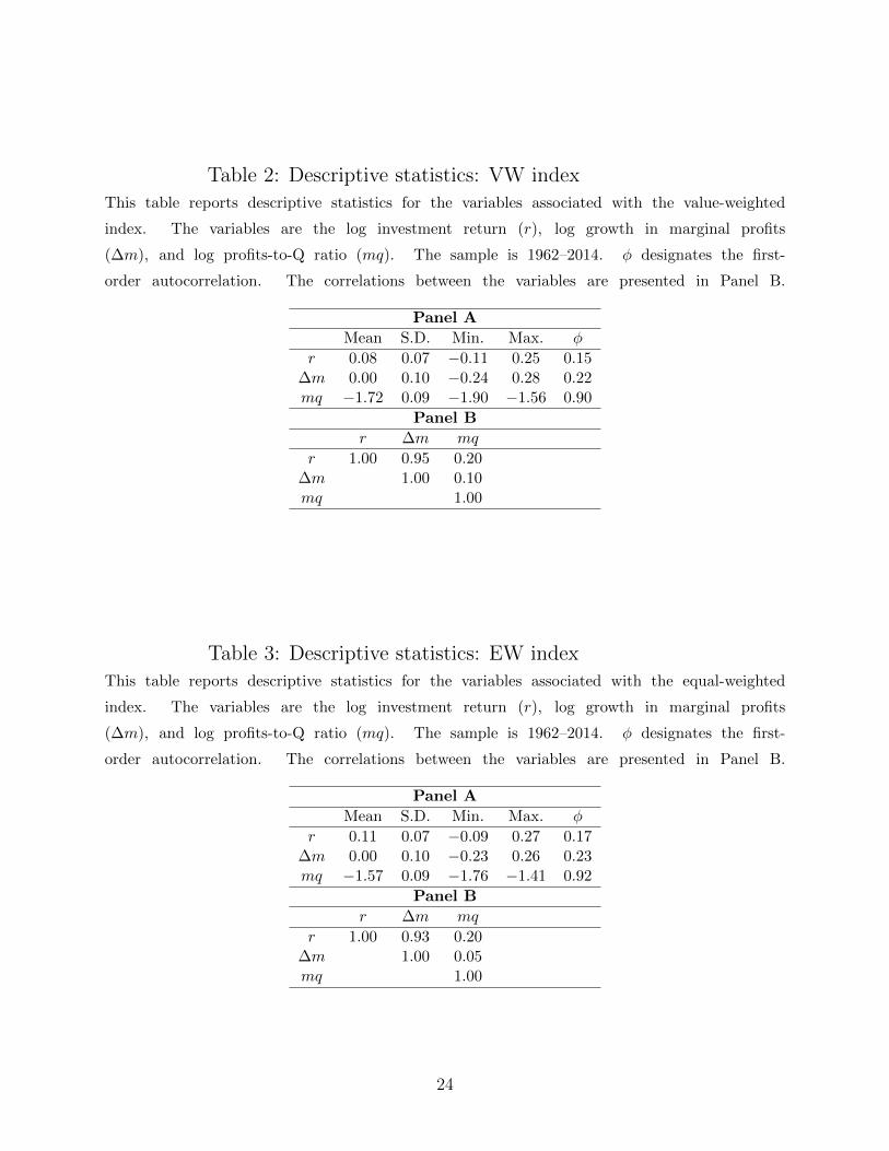
Table 2: Descriptive statistics: VW indexThis table reports descriptive statistics for the variables associated with the value-weighted
index. The variables are the log investment return (r), log growth in marginal profits
(∆m), and log profits-to-Q ratio (mq). The sample is 1962–2014. φ designates the first-
order autocorrelation. The correlations between the variables are presented in Panel B.
Panel A
Mean S.D. Min. Max. φ
r 0.08 0.07 −0.11 0.25 0.15∆m 0.00 0.10 −0.24 0.28 0.22mq −1.72 0.09 −1.90 −1.56 0.90
Panel B
r ∆m mq
r 1.00 0.95 0.20∆m 1.00 0.10mq 1.00
Table 3: Descriptive statistics: EW indexThis table reports descriptive statistics for the variables associated with the equal-weighted
index. The variables are the log investment return (r), log growth in marginal profits
(∆m), and log profits-to-Q ratio (mq). The sample is 1962–2014. φ designates the first-
order autocorrelation. The correlations between the variables are presented in Panel B.
Panel A
Mean S.D. Min. Max. φ
r 0.11 0.07 −0.09 0.27 0.17∆m 0.00 0.10 −0.23 0.26 0.23mq −1.57 0.09 −1.76 −1.41 0.92
Panel B
r ∆m mq
r 1.00 0.93 0.20∆m 1.00 0.05mq 1.00
24

Table 4: VAR estimatesThis table reports the VAR(1) estimation results when the predictor is the profits-to-Q ra-
tio. The variables in the VAR are the log investment return (r), log growth in marginal prof-
its (m), and log profits-to-Q ratio (mq). The results in Panels A and B correspond to the
value- and equal-weighted investment returns, respectively. b denote the VAR slopes associ-
ated with lagged mq, while t denotes the respective Newey and West (1987) t-statistics (calcu-
lated with one lag). R2 is the coefficient of determination for each equation in the VAR, in
%. blr denote the long-run coefficients (infinite horizon). t(blrr = 0) and t(blrr = 1) denote the
t-statistics associated with the null hypotheses (blrr = 0, blrm = −1) and (blrr = 1, blrm = 0), re-
spectively. The full sample corresponds to annual data for the 1962–2014 period. Italic, under-
lined, and bold numbers denote statistical significance at the 10%, 5%, and 1% levels, respectively.
b t R2 blr t(blrr = 0) t(blrr = 1)
Panel A (VW)
r −0.06 −0.48 0.01 −0.26 −0.53 −2.57∆m −0.31 −1 .71 0.07 −1.24 −0.50 −2.53mq 0.90 13.42 0.81
Panel B (EW)
r 0.01 0.10 0.00 0.05 0.10 −1 .92∆m −0.24 −1.48 0.06 −0.94 0.13 −1 .87mq 0.92 16.39 0.85
25

Figure 1: Marginal profits-to-Q ratioThis figure plots the time-series for the value-weighted (VW) and equal-
weighted (EW) marginal profits-to-Q ratio. The sample is 1962 to 2014.
26

Figure 2: Investment returnThis figure plots the time-series for the value-weighted (VW) and equal-
weighted (EW) investment return. The sample is 1962 to 2014.
Figure 3: Growth in marginal profitsThis figure plots the time-series for the value-weighted (VW) and equal-
weighted (EW) growth rate in marginal profits. The sample is 1962 to 2014.
27

Panel A (slopes)
Panel B (t-stats)
Figure 4: Direct term structure of predictive slopes: VW returnThis figure plots the term structure of multiple-horizon predictive coefficients, and respective t-
statistics, for the case of the value-weighted investment return. The predictive slopes are obtained
from weighted long-horizon regressions. The coefficients are associated with the log investment re-
turn (r), log growth in marginal profits (m), and log profits-to-Q ratio (mq). The forecasting vari-
able is mq in all three cases. “Sum” denotes the value of the variance decomposition, in %. The
long-run coefficients are measured in %, and K represents the number of years ahead. The hor-
izontal lines represent the 5% critical values (−1.96, 1.96). The original sample is 1962 to 2014.
28

Panel A (slopes)
Panel B (t-stats)
Figure 5: Direct term structure of predictive slopes: EW returnThis figure plots the term structure of multiple-horizon predictive coefficients, and respective t-
statistics, for the case of the equal-weighted investment return. The predictive slopes are obtained
from weighted long-horizon regressions. The coefficients are associated with the log investment re-
turn (r), log growth in marginal profits (m), and log profits-to-Q ratio (mq). The forecasting vari-
able is mq in all three cases. “Sum” denotes the value of the variance decomposition, in %. The
long-run coefficients are measured in %, and K represents the number of years ahead. The hor-
izontal lines represent the 5% critical values (−1.96, 1.96). The original sample is 1962 to 2014.
29

Panel A (slopes)
Panel B (t-stats)
Figure 6: Direct term structure of predictive slopes: alternative VW returnThis figure plots the term structure of multiple-horizon predictive coefficients, and respective t-statistics,
for the case of the alternative value-weighted investment return. The predictive slopes are obtained
from weighted long-horizon regressions. The coefficients are associated with the log investment re-
turn (r), log growth in marginal profits (m), and log profits-to-Q ratio (mq). The forecasting vari-
able is mq in all three cases. “Sum” denotes the value of the variance decomposition, in %. The
long-run coefficients are measured in %, and K represents the number of years ahead. The hor-
izontal lines represent the 5% critical values (−1.96, 1.96). The original sample is 1962 to 2014.
30

Panel A (slopes)
Panel B (t-stats)
Figure 7: Direct term structure of predictive slopes: alternative EW returnThis figure plots the term structure of multiple-horizon predictive coefficients, and respective t-statistics,
for the case of the alternative equal-weighted investment return. The predictive slopes are obtained
from weighted long-horizon regressions. The coefficients are associated with the log investment re-
turn (r), log growth in marginal profits (m), and log profits-to-Q ratio (mq). The forecasting vari-
able is mq in all three cases. “Sum” denotes the value of the variance decomposition, in %. The
long-run coefficients are measured in %, and K represents the number of years ahead. The hor-
izontal lines represent the 5% critical values (−1.96, 1.96). The original sample is 1962 to 2014.
31

Panel A (slopes)
Panel B (t-stats)
Figure 8: VAR-based term structure of predictive slopes: VW returnThis figure plots the term structure of multiple-horizon predictive coefficients, and respective t-statistics, for
the case of the value-weighted investment return. The predictive slopes are obtained from a first-order VAR.
The coefficients are associated with the log investment return (r), log growth in marginal profits (m), and log
profits-to-Q ratio (mq). The forecasting variable is mq in all three cases. “Sum” denotes the value of the vari-
ance decomposition, in %. The long-run coefficients are measured in %, and K represents the number of years
ahead. The horizontal lines represent the 5% critical values (−1.96, 1.96). The original sample is 1962 to 2014.
32

Panel A (slopes)
Panel B (t-stats)
Figure 9: VAR-based term structure of predictive slopes: EW returnThis figure plots the term structure of multiple-horizon predictive coefficients, and respective t-statistics, for
the case of the equal-weighted investment return. The predictive slopes are obtained from a first-order VAR.
The coefficients are associated with the log investment return (r), log growth in marginal profits (m), and log
profits-to-Q ratio (mq). The forecasting variable is mq in all three cases. “Sum” denotes the value of the vari-
ance decomposition, in %. The long-run coefficients are measured in %, and K represents the number of years
ahead. The horizontal lines represent the 5% critical values (−1.96, 1.96). The original sample is 1962 to 2014.
33

References
Abel, A.B., and O.J. Blanchard, 1986, The present value of profits and cyclical movements
in investment, Econometrica 54, 249–273.
Asimakopoulos, P., S. Asimakopoulos, N. Kourogenis, and E. Tsiritakis, 2014, Time-
disaggregated dividend-price ratio and dividend growth predictability in large equity
markets, Journal of Financial and Quantitative Analysis, forthcoming.
Barro, R.J., 1990, The Stock market and investment, Review of Financial Studies 3, 115-31.
Belo, F., C. Xue, and L. Zhang, 2013, A supply approach to valuation, Review of Financial
Studies 26, 3029–3067.
Binsbergen, J.H., and R.S. Koijen, 2010, Predictive regressions: A present-value approach,
Journal of Finance 65, 1439–1471.
Bloom, N., 2009, The impact of uncertainty shocks, Econometrica 77, 623–685.
Blume, M.E., F. Lim, and A.C. MacKinlay, 1998, The declining credit quality of U.S. cor-
porate debt: Myth or reality? Journal of Finance 53, 1389–1413.
Campbell, J.Y., and R.J. Shiller, 1988, The dividend price ratio and expectations of future
dividends and discount factors, Review of Financial Studies 1, 195–228.
Chen, L., 2009, On the reversal of return and dividend growth predictability: A tale of two
periods, Journal of Financial Economics 92, 128–151.
Chen, L., Z. Da, and B. Larrain, 2016, What moves investment growth? Journal of Money,
Credit and Banking 48, 1613–1653.
Chen, L., Z. Da, and R. Priestley, 2012, Dividend smoothing and predictability, Management
Science 58, 1834–1853.
Cochrane, J.H., 1991, Production-based asset pricing and the link between stock returns and
economic fluctuations, Journal of Finance 46, 209–237.
34

Cochrane, J.H., 1992, Explaining the variance of price-dividend ratios, Review of Financial
Studies 5, 243–280.
Cochrane, J.H., 2008, The dog that did not bark: A defense of return predictability, Review
of Financial Studies 21, 1533–1575.
Cochrane, J.H., 2011, Presidential address: Discount rates, Journal of Finance 66, 1047–
1108.
Cohen, R.B., C. Polk, and T. Vuolteenaho, 2003, The value spread, Journal of Finance 58,
609–641.
Cooper, R.W., and J.C. Haltiwanger, 2006, On the nature of capital adjustment costs,
Review of Economic Studies 73, 611–633.
Cooper, I., and R. Priestley, 2016, The expected returns and valuations of private and public
firms, Journal of Financial Economics 120, 41–57.
Engsted, T., T.Q. Pedersen, and C. Tanggaard, 2012, The log-linear return approximation,
bubbles, and predictability, Journal of Financial and Quantitative Analysis 47, 643–665.
Erickson, T., and T.M. Whited, 2000, Measurement error and the relationship between
investment and q, Journal of Political Economy 108, 1027–1057.
Fama, E.F., and K.R. French, 1988, Dividend yields and expected stock returns, Journal of
Financial Economics 22, 3–25.
Fama, E.F., and K.R. French, 1995, Size and book-to-market factors in earnings and returns,
Journal of Finance 50, 131–155.
Hayashi, F., 1982, Tobin’s marginal q and average q: A neoclassical interpretation, Econo-
metrica 50, 213–224.
Hennessy, C.A., and T.M. Whited, 2007, How costly is external financing? Evidence from a
structural estimation, Journal of Finance 62, 1705–1745.
35

Hribar, P., and P. Quinn, 2013, Managers and investor sentiment, Working paper, University
of Iowa.
Koijen, R.S.J., and S. Van Nieuwerburgh, 2011, Predictability of returns and cash flows,
Annual Review of Financial Economics 3, 467–491.
Larrain, B., and M. Yogo, 2008, Does firm value move too much to be justified by subsequent
changes in cash flow? Journal of Financial Economics 87, 200–226.
Lettau, M., and S. Ludvigson, 2002, Time-varying risk premia and the cost of capital: An
alternative implication of the Q theory of investment, Journal of Monetary Economics
49, 31–66.
Lettau, M., and S. Van Nieuwerburgh, 2008, Reconciling the return predictability evidence,
Review of Financial Studies 21, 1607–1652.
Liu, L.X., T.M. Whited, and L. Zhang, 2009, Investment-based expected stock returns,
Journal of Political Economy 117, 1105–1139.
Maio, P., 2013, The “Fed model” and the predictability of stock returns, Review of Finance
17, 1489–1533.
Maio, P., and P. Santa-Clara, 2015, Dividend yields, dividend growth, and return predictabil-
ity in the cross-section of stocks, Journal of Financial and Quantitative Analysis 50,
33–60.
Morck, R., A. Shleifer, and R. Vishny, 1990, The stock market and investment: Is the market
a sideshow? Brookings Papers on Economic Activity 2, 157–215.
Newey, W.K., and K.D. West, 1987, A simple, positive semi-definite, heteroskedasticity and
autocorrelation consistent covariance matrix, Econometrica 55, 703–708.
Rangvid, J., M. Schmeling, and A. Schrimpf, 2014, Dividend predictability around the world,
Journal of Financial and Quantitative Analysis 49, 1255–1277.
36

Tobin, J., 1969, A general equilibrium approach to monetary theory, Journal of Money,
Credit, and Banking 1, 15–29.
37