IJOPCM-2018 Grid Distortion Errors

Int. J. Open Problems Compt. Math., Vol. 11, No. 4, December 2018 ISSN 1998-6262; Copyright © ICSRS Publication, 2018 www.i-csrs.org

Grid distortion errors in streamfunction coordinates

M.H. Hamdan, M.A. Hajji, R.A. Ford, M.S. Abu Zaytoon

Department of Mathematics Statistics, University of New Brunswick,

P.O. Box 5050, Saint John, New Brunswick, Canada E2L 4L5 e-mail:

[email protected]

Department of Mathematical

Sciences, UAE University,

P.O. Box 15551, Al Ain, UAE

e-mail:

[email protected]

School of Information Technology, College of the North Atlantic –

Qatar,

P.O. Box 24449, Doha, Qatar

e-mail:

[email protected]

Mechanical Engineering Division, Higher Colleges of Technology,

P.O. Box 41012, Abu Dhabi, UAE

e-mail:

[email protected]

Abstract

Grid distortion errors arising due to the use of non-orthogonal grid in the curvilinear streamfunction coordinate system are analyzed in this work. The objective is to offer a method of measuring and quantifying grid distortion errors. This is accomplished by solving numerically the problem of viscous fluid flow in a curvilinear, two-dimensional channel, governed the the Navier-Stokes equations. The curvilinear flow domain is transformed into a rectangular computational domain, and the governing equations and boundary conditions are transformed, using the von Mises transformation. Grid distortions errors are then quantified using the metrics of transformation, and are taken to be proportional to the angle of inclination to the horizontal of the tangents to the streamlines of the flow. At each grid cell the sine of the inclination angle, defined in terms of the metrics, is computed and the largest possible value is obtained. Effects of the various boundary vorticity approximations on grid distortion are studied in this work where in the process the streamline pattern in the flow

(Communicated by Iqbal Jebril)

M.H. Hamdan et al. 88

field and the equivorticity curves are obtained for small Re when uniform and non-uniform grids are used.

Keywords: Grid distortion errors; von Mises; curvilinear coordinates.

1 Introduction When finite differences are used to solve partial differential equations with boundary conditions in general coordinate systems (such as fluid flow equations in curvilinear domains), the following are some of the errors and their sources that are introduced in the process and affect the local and global accuracies of the numerical solution obtained (cf. [1-5] and the references therein):

a) Round-off errors due to numerical computations b) Solution errors due to the differencing schemes c) Errors in the approximation of boundary conditions d) Local grid distortion errors due to loss of orthogonality of grid when

curvilinear coordinates are used e) Errors due to high grid aspect ratios f) Additional truncation errors that arise due to the introduction of extra

convective terms when using curvilinear coordinates.

In addition to the above, grid size used, grid clustering near the boundary, the order of accuracy of the differencing schemes used in the computational domain and on the boundary, and the choice of uniform or non-uniform (clustered) grid, influence both the local and global accuracy of the numerical solution. The above factors have been the subject matter of a large number of investigations (cf. [6-15] and the references therein), due to the importance of these studies in the efficient design of software and codes with applications to fluid flow and groundwater simulation, [14]. Errors associated with grid distortion are due to the use of non-orthogonal grid and the mapping of a curvilinear region onto a rectangular region. These errors can be measured in terms of angles of deviation from orthogonality of a computational grid. Their influence on local and global accuracies of computed solutions can be quantified in terms of the metrics of the employed transformation by defining the deviation angle in terms of the metrics. Grid distortion errors are therefore dependent in part on: (i) the transformation used, (ii) the shape of the curvilinear boundary, and (iii) the type of grid employed (that is, whether clustered or uniform). In using uniform grid, it is sometimes possible to arrive at the wrong conclusion that uniform grid produce small grid distortion. If, when using uniform grid, the step size near the boundary is fairly large (non-refined grid) then the effect of the boundary shape is not properly transmitted into the whole computational domain.

89 Grid distortion errors in streamfunction

This results in a superficial reduction in grid distortion error. For clustered grid with small step size near the boundary, a more accurate effect of the boundary is transmitted into the computational domain and the effect of grid distortion is more pronounced. In the current work we study grid distortion and the main factors that have an influence on it when the curvilinear domain is mapped onto a rectangular domain using von Mises coordinates, by devising a numerical experiment in which we consider viscous fluid flow through a two-dimensional curvilinear channel. We determine in the computational domain the largest grid distortion errors incurred when different boundary shapes are used and different finite difference approximations are implemented in computing vorticity at the boundaries. Comparison is provided between grid distortion errors when a uniform grid is used and when a grid with a variable step size is used. Grid size used is taken the same for all cases studied and first, second and third-order accurate boundary vorticity schemes are used for the sake of comparison. However, we also study the effect of grid refinement on grid distortion. To measure the effectiveness of a particular boundary we consider the region near the entrance to the channel. It is expected that the parabolic inlet profile is undisturbed in the first few steps into the channel. This implies that the vorticity along each streamline is constant, and the equivorticity lines should be as close to the horizontal as possible. However, due to boundary vorticity approximations and the influence of boundary shape, the flow pattern is disturbed and the equivorticity lines deviate from the horizontal. In order to place a quantitative measure on the influence of the boundary vorticity approximations, we measure the grid distortion in terms of sine of the angle between the horizontal axis and the tangent to the streamlines of the flow. In the process we solve the governing Navier-Stokes equations, generate streamline patterns and equivorticity curves.

2 Metrics of transformation Consider the curvilinear net in which the curves constant, represent streamlines of the flow. Now, consider the following transformation which defines the von Mises coordinates [16-18]:

. (1)

The Jacobian of transformation (1) is defined as

),( yx =y

þýü

==

),( yxyyxx


, (2)

where subscript notation denotes partial differentiation. Let be an element of arc length along any curve in the plane, with the squared element of arc length given by: . (3) From (1) we obtain:

. (4)

Using (4) in (3), we obtain: , (5) where , and are the metrics of transformation (coefficients of the first fundamental form) that satisfy: , (6) , (7)

(8) Distances in the and directions are given, respectively, by: , (9)

, (10) and the Jacobian of transformation (2) is expressed in terms of the metrics as

. (11) If fluid flows along the streamline in the direction of increasing x, then

and the positive sign in (11) is chosen, while if fluid flows in the direction of decreasing x, then and the negative sign in (11) is chosen. Now, the

yyy

xyxJ =

¶¶

=),(),(

dS -xy

222 dydxdS +=

þýü

+==

)yydydxydydxdx

x

222 ),(),(2),( yyyyy dxGdxdxFdxxEdS ++=

FE, G

2)(1),( xyxE +=y

yyyyxF x=),(

.)(),( 2yy yxG =

-x -y

dxEdSx =yy dEdS =

2FEGJ -= !

c=y0>J

0<J


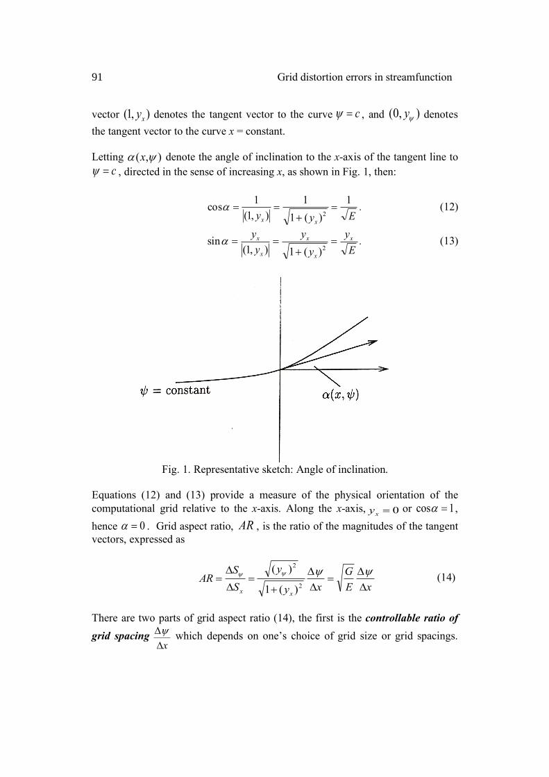
vector denotes the tangent vector to the curve , and denotes the tangent vector to the curve x = constant. Letting denote the angle of inclination to the x-axis of the tangent line to

, directed in the sense of increasing x, as shown in Fig. 1, then:

. (12)

. (13)

Fig. 1. Representative sketch: Angle of inclination.

Equations (12) and (13) provide a measure of the physical orientation of the computational grid relative to the x-axis. Along the x-axis, or , hence . Grid aspect ratio, , is the ratio of the magnitudes of the tangent vectors, expressed as

(14)

There are two parts of grid aspect ratio (14), the first is the controllable ratio of grid spacing which depends on one’s choice of grid size or grid spacings.

),1( xy c=y ),0( yy

),( ya xc=y

Eyyxx

1)(1

1),1(

1cos2=

+==a

Ey

yy

yy x

x

x

x

x =+

==2)(1),1(

sina

0=xy 1cos =a0=a AR

xEG

xy

ySS

ARxx D

D=

DD

+=

D

D=

yyyy

2

2

)(1

)(

xDDy


The second is the uncontrollable ratio , which is inherent in the

curvilinear coordinate system used. The local grid distortion is determined by angle between the coordinate lines, measured by:

. (15)

Accuracy of the solution is degraded by this grid distortion. Therefore, for high accuracy, the grid should be orthogonal or near orthogonal. For orthogonal grid,

or . Equivalently, , which implies that

or . If then (which is impossible), while if then .If the grid is not orthogonal, additional truncation errors are introduced and are proportional to . However, it is generally accepted that

departure from orthogonality of up to radians can be tolerated, [1].

3 Numerical experiment 3.1 Physical domain quantities and equations

In order to study the effect of grid distortion, error propagation, accuracy of the numerical solution and convergence of the numerical scheme used, we consider the flow of a viscous fluid through a two-dimensional channel shown diagrammatically in Fig. 2, and described by: (16)

Fluid enters through section ad and exists through bc. The channel is assumed to be long enough to impose parallel flow at its inlet and exit.

2

2

)(1

)(

xy

y

+

y

apJ -=2

EGF

yy

x

x =+

==2)(1

sincos aJ

2pJ = 0sincos == aJ 0== yyyF x

0=xy 0=yy 0=yy 0=AR 0=xyyyAR =

Jcos

4p

)}()(;),{( 21maxmin xfyxfxxxyx ££££


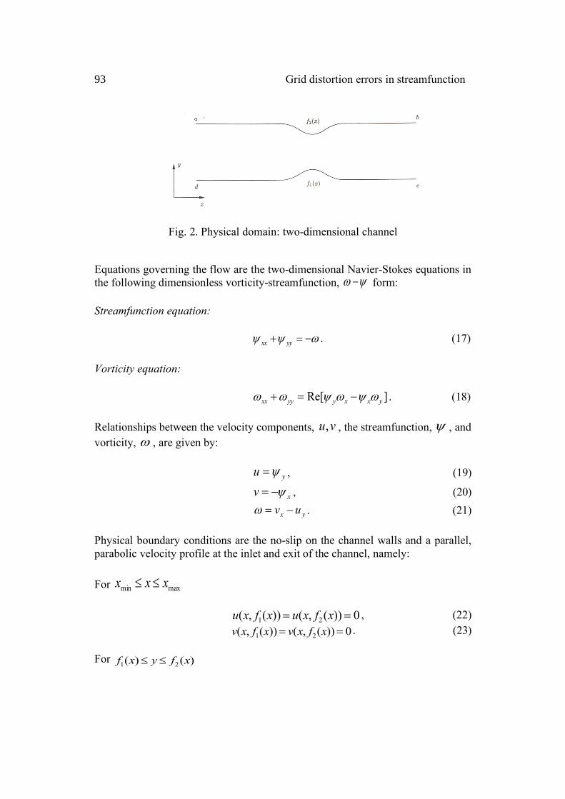
Fig. 2. Physical domain: two-dimensional channel

Equations governing the flow are the two-dimensional Navier-Stokes equations in the following dimensionless vorticity-streamfunction, form: Streamfunction equation: . (17) Vorticity equation: . (18) Relationships between the velocity components, , the streamfunction, , and vorticity, , are given by: , (19)

, (20) . (21) Physical boundary conditions are the no-slip on the channel walls and a parallel, parabolic velocity profile at the inlet and exit of the channel, namely: For

, (22) . (23)

For

yw -

wyy -=+ yyxx

]Re[ yxxyyyxx wywyww -=+

vu, yw

yu y=

xv y-=

yx uv -=w

maxmin xxx ££

0))(,())(,( 21 == xfxuxfxu0))(,())(,( 21 == xfxvxfxv

)()( 21 xfyxf ££


, (24) at and . (25)

Corresponding conditions on the streamfunction and vorticity are the following inlet and exit conditions: For

, (26)

. (27)

For , (28) , (29) , (30)

. (31)

3.2 Computational domain quantities and equations

In order to solve the governing equations using finite differences, the curvilinear physical domain is mapped onto a rectangular computational domain, Fig. 3, using the von Mises transformation (1). Boundary conditions and governing equations are transformed into von Mises coordinates, as described in what follows. Using transformation (1), the roles of and y are interchanged, the curvilinear streamlines, constant, in the physical domain are horizontal straight lines in the computational domain, and the physical domain is mapped onto the rectangular computational domain described by: (32)

2maxmin 1),(),( yyxuyxu -==

0== xvv ),( min yx ),( max yx

)()( 21 xfyxf ££

3),(),(

3

maxminyyyxyx -==yy

yyxyx 2),(),( maxmin ==ww

maxmin xxx ££

min1 ))(,( yy =xfxmax2 ))(,( yy =xfx

)(1 1)())(,( xfyyx uvxfx =-=w

)(2 2)())(,( xfyyx uvxfx =-=w

y=y

};),{( maxminmaxmin yyyy ££££ xxxx


Fig. 3. Rectangular Computational domain.

It is clear that the lower and upper boundaries are the streamlines and , respectively. First-order partial differential operators in the Cartesian and von Mises coordinate systems are related by:

, (33)

, (34)

and higher-order operators can be obtained by repeated applications of (33) and (34) onto themselves. Governing equations (17) and (18) are thus transformed into the following forms, to be solved for and : The equation: . (35)

The equation: , (36) where . (37)

Velocity components take the following forms in von Mises coordinates

miny maxy

yy

¶-¶=¶yyx

xx

yy

¶=¶yy1

),( yxy ),( yw x

-y

3)(][ yw yyL =

-w

xyyL wwww yy yRe)(][ 2 +=

yyyyy ¶++¶-¶º ])(1[2)( 22xxxxx yyyyL


, (38)

(39)

and the square of the speed of the flow is given by:

. (40)

Equations (35) and (36) are to be solved in the computational domain subject to the following transformed conditions on and : For

, (41) , (42)

, (43)

. (44)

For

, (45)

, (46)

, (47)

. (48)

4 Finite difference approximations 4.1 Discretizing the flow domain

In order to solve (35) and (36) numerically, subject the transformed boundary conditions (41)-(48), the computational domain is discretized using either a uniform grid or a non-uniform grid, with vertical grid lines ranging from i=1 at

yyu 1=

.xx uyyy

v ==y

2

2222

)()(1

yyyvuq x+

=+=

),( yxy ),( yw x

maxmin xxx ££

)(),( 1min xfxy =y)(),( 2max xfxy =y

),(2

min min)(

21),( yyyw xx qvx -=

),(2

max max)(

21),( yyyw xx qvx -=

maxmin yyy ££

yy

y =-3

),(),( min3

minxyxy

yy

y =-3

),(),( max3

maxxyxy

),(2),( minmin yyw xyx =),(2),( maxmax yyw xyx =


to i=Imax at , and horizontal grid lines ranging from j=1 at to j=Jmax at . In this work, we choose the following data for the computational domain:

; (49)

; (50)

where k is a shape parameter that controls the thickness of the boundary bump, and

The horizontal extent of the channel is deemed to be sufficient to impose parallel inlet and exit velocity profiles. We select Imax = 201 grid points in the x-direction and Jmax = 51 grid points in the -direction. In using uniform grid, step sizes are constant and take the values and

. The choice of constant step size in the -direction in the computational domain produces a grid in the physical domain that is clustered near the horizontal centerline of the channel, away from the boundary, [3,4]. This is a disadvantage of using uniform grid, since one desires clustering near the boundary in order to better capture boundary effects. In using non-uniform grid, a convenient way of generating clustered grid near the computational boundary is to select in the physical domain constant steps in the y-direction and to use (26) to compute the -values in the computational domain, hence determine the step sizes in the -direction. This method produces a naturally clustered grid near the computational boundary that is tied to the inlet velocity profile [3]. This is one of the advantages of using the von Mises transformation. Now, at the inlet to the channel, , and using 51 grid points in the y-direction gives in the physical domain. We can then generate the set of y-values {-1, -0.96, -0.92, …, 1} and calculate the

corresponding using (26). We generate values for the variable step sizes using the three grid points , by defining for j = 2 to Jmax-1:

minx maxx minymaxy

îíì

£++->-

=1);cos1(1

1;1)(1 xxk

xxf

p maxmin xxx ££

îíì

£+->

=1);cos1(1

1;1)(2 xxk

xxf

p maxmin xxx ££

.32;

32;4;4 maxminmaxmin =-==-= yyxx

y

04.0=Dx0267.0»Dy y

yy

11 ££- y04.0=Dy

== }51,...,2,1;{ jy j

jyjyD

)1,(),,(),1,( +- jijiji


, (51)

. (52)

4.2 Discretizing the governing equations

Expansion of a function about the point and using Taylor series approximations, we obtain the following second-order finite difference expressions for the first and second derivatives with respect to and , valid for variable step size in the -direction:

, (53)

, (54)

, (55)

, (56)

, (57)

where stands for either of the unknowns or , and

. (58)

Applying approximations (53)-(58) to the and equations (35) and (36), we obtain discretized forms of the equations which are then written in the following tri-diagonal matrix form that is suitable for Successive Line Over Relaxation (SLOR) in the j-direction with sweep in the i-direction:

, (59)

jjj yyy -=D +1

11 -- -=D jjj yyy

),( yxF ),( ji

x yy

xFF

xF jiji

ji D

-»

¶¶ -+

2,1,1

,

1

1,1,

, -

-+

D+D

-»

¶¶

jj

jiji

ji

FFFyyy

2,1,,1

,2

2 2x

FFFxF jijiji

ji D

+-»

¶¶ -+

÷÷ø

öççè

æ

DD+D

++-»

¶¶

-

-+

12

1,,1,

,2

2 )1(2

jjj

jijjijji

ji

FFFFyyybb

y

1

1,11,11,11,1

,

2

22 -

+--+--++

DD+DD--+

»¶¶¶

jj

jijijiji

ji xxFFFF

xF

yyy

F w y

1-DD

=j

jj y

yb

-y -w

jijijijijijiji BFcFbFa ,1,,,,1,, =++ +-


where stands for or , and is the right-hand-side vector. The

matrix coefficients , and the right-hand-side vector are given for each of governing equations (35) and (36) in what follows, for i=2,3,…,Imax-1, and j=2,3,…,Jmax-1. For the y-equation:

(60)

(61)

(62)

(63)

For the -equation:

(64)

(65)

(66)

(67)

jiF , jiy , ji,w jiB ,

jijiji cba ,,, ,,jiB ,

( ){ }2,1,12

, )(41 jijijji yyxa -+ -+D+= b

( ) { }2,1,12

22

1,1,, )(41

)(4 jijij

jjijiji yyxyyb -+-+ -+D

+---=

bb

{ }2,1,12

, )(41

jijij

jji yyxc -+ -+D÷

÷ø

öççè

æ +=

bb

{ }1,11,11,11,11,1,,1,1

,3

1,1,1

2

,1,12

1,1,,

))((

)(2)()(2

+--+--++-+-+

-+-

-+-+

--+--+

-÷÷ø

öççè

æ

D+DD

++--=

jijijijijijijiji

jijijijj

jijijijiji

yyyyyyyy

yyxyyyyB wyy

w

])2

(1)[(2 2,1,11,

jijijjjji

yya -+

-

-+D+D= yyb

])2

(1)[)(1(2)(2 2,1,11

21,1,,

jijijjjjijiji

yyyyb -+

--+

-+D+D+---= yyb

])2

(1)[(2 2,1,11,

jijijjji

yyc -+

-

-+D+D= yy

þýü

îíì --+

--+

--D+DD

+

ïþ

ïýü

ïî

ïíì

+--D+D

D-=

+--+--++-+-+

-+-+-

-+-+-

-+

2))((

))()((2Re

)()()(

1,11,11,11,11,1,,1,1

,1,11,1,1

,1,11,1,,1

22

1,1,,

jijijijijijijiji

jijijijijj

jijijijijijj

jijiji

yyyy

yyx

xyyB

wwww

wwyy

wwwwwyy


4.3 Boundary vorticity approximations

Vorticity on the lower and upper boundaries is given by (43) and (44), respectively, in terms of the first derivative of the square of the speed of the flow. Boundary vorticity is approximated using the following finite difference expressions of first, second and third order accuracy for the first derivative of the square of the speed, for both uniform and non-uniform grid. For first-order accurate approximation we implement 2, 3, 4, and 5 grid points using schemes derived in [4]. Reference to these schemes is as follows: a (1,2) scheme uses the grid points along j=1 and j=2, while a (1,2,3,4,5) scheme uses grid points along j=1,2,3,4,5.

For non-uniform grid, first, second and third-order accurate forward schemes, respectively, using the natural order of grid lines, are: First-order Schemes: (1,2) Scheme

. (68)

(1,2,3) Scheme

(69)

(1,2,3,4) Scheme

(70)

(1,2,3,4,5) Scheme

(71)

Second-order (1,2,3) Scheme

(72)

1

1,2

2,2

1,2

1,)()(

21)(

21

yw y

D-

-»-= iiii

qqq

21

1,2

2,2

3,2

1,2

1, 2)(2)()(

21)(

21

yyw y

D+D-+

-»-= iiiii

qqqq

321

1,2

2,2

3,2

4,2

1,2

1, 23)(3)()()(

21)(

21

yyyw y

D+D+D-++

-»-= iiiiii

qqqqq

4321

1,2

2,2

3,2

4,2

5,2

1,2

1, 234)(4)()()()(

21)(

21

yyyyw y

D+D+D+D-+++

-»-= iiiiiii

qqqqqq

])(

)()()2([

21)(

21 2

3,221

122,

21

2121,

211

211,

21, iiiii qqqq

yyyy

yyyy

yyyyyw y

DD+DD

-DDD+D

+D+DDD+D

--»-=


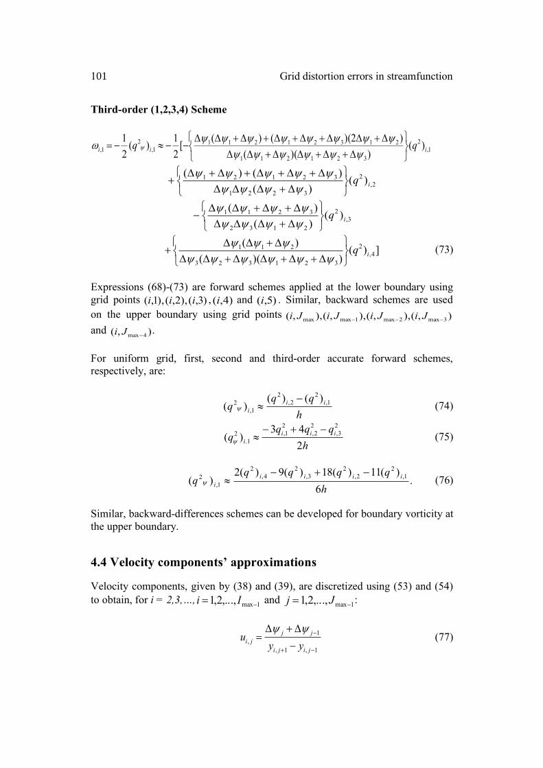
Third-order (1,2,3,4) Scheme

(73)

Expressions (68)-(73) are forward schemes applied at the lower boundary using grid points , and . Similar, backward schemes are used on the upper boundary using grid points and . For uniform grid, first, second and third-order accurate forward schemes, respectively, are:

(74)

(75)

(76)

Similar, backward-differences schemes can be developed for boundary vorticity at the upper boundary.

4.4 Velocity components’ approximations

Velocity components, given by (38) and (39), are discretized using (53) and (54) to obtain, for i = 2,3,…, and :

(77)

1,2

321211

213212111,

21, )(

))(()2)(()([

21)(

21

iii qqþýü

îíì

D+D+DD+DDD+DD+D+D+D+DD

--»-=yyyyyy

yyyyyyyyw y

2,2

3221

32121 )()(

)()(iq

þýü

îíì

D+DDDD+D+D+D+D

+yyyy

yyyyy

3,2

2132

3211 )()()(

iqþýü

îíì

D+DDDD+D+DD

-yyyyyyyy

])())((

)(4,

2

321323

211iq

þýü

îíì

D+D+DD+DDD+DD

+yyyyyy

yyy

)3,(),2,(),1,( iii )4,(i )5,(i),(),,(),,(),,( 3max2max1maxmax --- JiJiJiJi

),( 4max-Ji

hqq

q iii

1,2

2,2

1,2 )()()(

-»y

hqqq

q iiii 2

43)(

23,

22,

21,

1.2 -+-

»y

.6

)(11)(18)(9)(2)( 1,

22,

23,

24,

2

1,2

hqqqq

q iiiii

-+-»y

1max,...,2,1 -= Ii 1max,...,2,1 -= Jj

1,1,

1,

-+

-

-D+D

=jiji

jjji yy

uyy


(78)

or

(79)

For uniform grid, equations (77) and (79) take the forms, respectively:

(80)

(81)

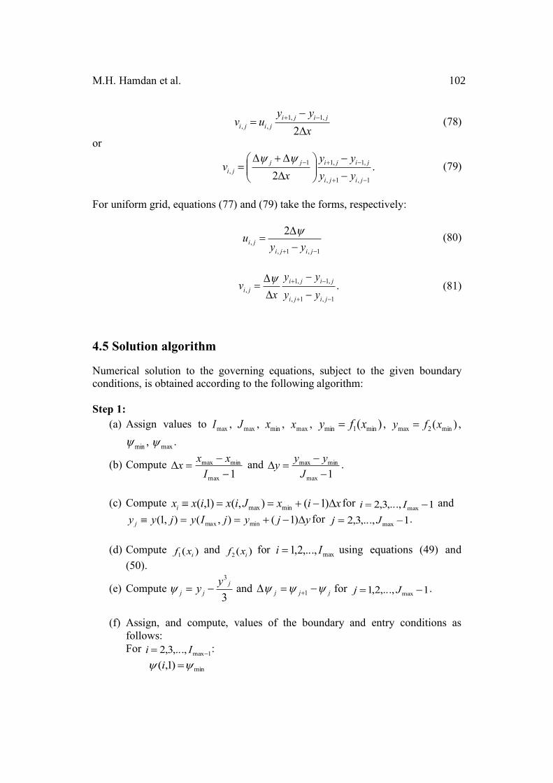
4.5 Solution algorithm

Numerical solution to the governing equations, subject to the given boundary conditions, is obtained according to the following algorithm: Step 1:

(a) Assign values to , , , , , , , .

(b) Compute and .

(c) Compute for and

for .

(d) Compute and for using equations (49) and (50).

(e) Compute and for .

(f) Assign, and compute, values of the boundary and entry conditions as

follows: For :

xyy

uv jijijiji D

-= -+

2,1,1

,,

.2 1,1,

,1,11,

-+

-+-

-

-÷÷ø

öççè

æD

D+D=

jiji

jijijjji yy

yyx

vyy

1,1,,

2

-+ -D

=jiji

ji yyu y

.1,1,

,1,1,

-+

-+

-

-

DD

=jiji

jijiji yy

yyx

v y

maxI maxJ minx maxx )( min1min xfy = )( min2max xfy =

miny maxy

1max

minmax

--

=DI

xxx1max

minmax

--

=DJ

yyy

xixJixixxi D-+==º )1(),()1,( minmax 1,...,3,2 max -= IiyjyjIyjyy j D-+==º )1(),(),1( minmax 1,...,3,2 max -= Jj

)(1 ixf )(2 ixf max,...,2,1 Ii =

3

3j

jjyy -=y jjj yyy -=D +1 1,...,2,1 max -= Jj

1max,...,3,2 -= Ii

min)1,( yy =i


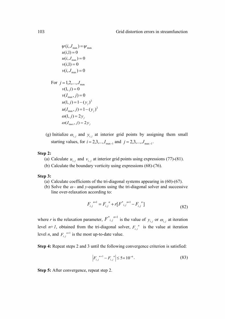
For

(g) Initialize and at interior grid points by assigning them small

starting values, for and . Step 2:

(a) Calculate and at interior grid points using expressions (77)-(81). (b) Calculate the boundary vorticity using expressions (68)-(76).

Step 3:

(a) Calculate coefficients of the tri-diagonal systems appearing in (60)-(67). (b) Solve the - and y-equations using the tri-diagonal solver and successive

line over-relaxation according to:

(82)

where r is the relaxation parameter, is the value of or at iteration level n+1, obtained from the tri-diagonal solver, is the value at iteration level n, and is the most up-to-date value. Step 4: Repeat steps 2 and 3 until the following convergence criterion is satisfied:

. (83)

Step 5: After convergence, repeat step 2.

maxmax ),( yy =Ji0)1,( =iu0),( max =Jiu

0)1,( =iv0),( max =Jiv

max,...,2,1 Jj =0),1( =jv0),( max =jIv

2)(1),1( jyju -=2

max )(1),( jyjIu -=

jyj 2),1( =w

jyjI 2),( max =w

ji ,w jiy ,1max,...,3,2 -= Ii 1max,...,3,2 -= Jj

jiu , jiv ,

w

][ ,1

,*

,1

,nji

nji

nji

nji FFrFF -+= ++

1,

* +njiF jiy , ji ,w

njiF ,

1,

+njiF

6,

1, 105 -+ ´£- n

jinji FF


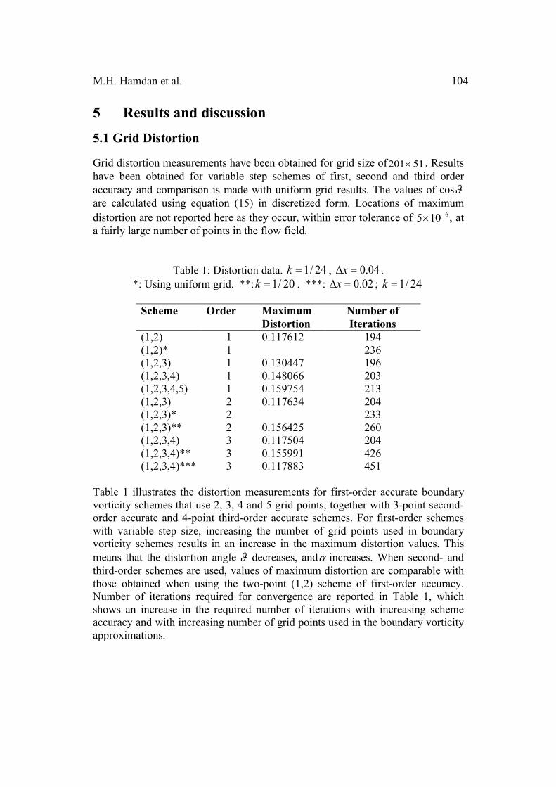
5 Results and discussion 5.1 Grid Distortion

Grid distortion measurements have been obtained for grid size of . Results have been obtained for variable step schemes of first, second and third order accuracy and comparison is made with uniform grid results. The values of are calculated using equation (15) in discretized form. Locations of maximum distortion are not reported here as they occur, within error tolerance of , at a fairly large number of points in the flow field.

Table 1: Distortion data. , . *: Using uniform grid. **: . ***: ;

Scheme Order Maximum

Distortion Number of Iterations

(1,2) 1 0.117612 194 (1,2)* 1 236 (1,2,3) 1 0.130447 196 (1,2,3,4) 1 0.148066 203 (1,2,3,4,5) 1 0.159754 213 (1,2,3) 2 0.117634 204 (1,2,3)* 2 233 (1,2,3)** 2 0.156425 260 (1,2,3,4) 3 0.117504 204 (1,2,3,4)** 3 0.155991 426 (1,2,3,4)*** 3 0.117883 451

Table 1 illustrates the distortion measurements for first-order accurate boundary vorticity schemes that use 2, 3, 4 and 5 grid points, together with 3-point second-order accurate and 4-point third-order accurate schemes. For first-order schemes with variable step size, increasing the number of grid points used in boundary vorticity schemes results in an increase in the maximum distortion values. This means that the distortion angle decreases, and increases. When second- and third-order schemes are used, values of maximum distortion are comparable with those obtained when using the two-point (1,2) scheme of first-order accuracy. Number of iterations required for convergence are reported in Table 1, which shows an increase in the required number of iterations with increasing scheme accuracy and with increasing number of grid points used in the boundary vorticity approximations.

51201´

Jcos

6105 -´

24/1=k 04.0=Dx20/1=k 02.0=Dx 24/1=k

J a


5.2 Effect of boundary shape

Equations (16) and (17) define the shape of the lower and upper channel boundaries. Thickness of the bump on the boundaries is controlled by parameter k. We have experimented with the following values: and found

that when selecting with non-uniform grid, an overflow error occurs. This

may be attributed to the closeness of streamlines to the boundary when the bump is thick, and the tendency of flow to approach separation threshold and the development of recirculating eddies near the leading and trailing edges. This kind of flow reversal changes the sign of the Jacobian of transformation, which is a drawback of using the von Mises transformation for viscous fluid flow. Results in

this work are therefore based on and , and Table 1 demonstrates

the increase in maximum grid distortion with increasing bump thickness when second- and third-order accurate boundary vorticity schemes are used.

5.3 Effect of grid refinement

If the number of grid points in the x-direction is doubled so that the grid size is and , the third-order accurate boundary vorticity scheme

produces a maximum distortion of 0.117883. Using this fine grid produces a slightly more accurate results. When using clustered grid, our numerical experiment showed that using grids containing more than 90 grid lines in the

direction results in no convergence. The upper limit on the grid size depends on the boundary vorticity finite difference formula used. For the third-order accurate scheme, the upper limit is 70 lines, while for the first-order accurate (1,2) scheme the limit is 102 lines. These upper limits represent the threshold for detection of viscous separation near the leading or trailing edges of the boundary bump, which results in flow reversal and a change of sign of the Jacobian, hence convergence is hindered.

5.4 Flow patterns and equivorticity curves

Results in this section are based on grid size of with boundary vorticity computed using third-order accurate schemes, for both uniform and non-uniform grids.

Streamlines of the flow for Re = 0 are illustrated in Fig. 4(a,b). For uniform grid, Fig. 4(a) demonstrates a loss of accuracy in the solution near the inlet and exit to the channel due to lack of clustering near the boundary. In using uniform grid, equal step sizes in the direction in the computational domain results in clustering near the centre of the channel and the boundary effects are not

241,

201,

181,

121

=k

201

>k

241

=k201

=k

51401´ 02.0=Dx

-y

51201´

-y


efficiently captured in the solution. In using non-uniform grid, Fig. 4(b), illustrates the steamline pattern with a more accurate, expected behaviour near the inlet and exit of the channel. We note that a non-uniform, clustered grid in the computational domain, with clustering near the boundary and capturing boundary effects more accurately, results in a uniform grid in the physical domain.

Streamline patterns have also been obtained for Re = 20 and 40, and exhibit similar qualitative behaviors to the patterns in Fig. 4(a,b), hence not shown here. However, effects of Re are better captured and illustrated in the equivorticity curves, shown in Fig. 5(a,b) and Fig. 6(a,b). As Re increases, the region between two equivorticity curves closest to the trailing edge gets larger. This is indicative of the possibility of potential viscous separation near the trailing edge, with increasing Re, and the potential formation of a recirculating eddy in that region. This behavior persists when either uniform or non-uniform grid is used. The effect of using non-uniform grid is, again, reflected in capturing the boundary effects better than uniform grid, hence producing different values of equivorticity curves near the boundary (along the same computational gridlines).

Fig. 4(a). Streamline pattern, uniform grid, Re = 0.


Fig. 4(b). Streamline pattern, clustered grid, Re = 0.

Fig. 5(a). Equivorticity curves, uniform grid, Re = 0.

Fig. 5(b). Equivorticity curves, clustered grid, Re = 0.


Fig. 6(a). Equivorticity curves, uniform grid, Re = 40.

Fig. 6(b). Equivorticity curves, clustered grid, Re = 40.

6 Conclusion In this work we studied grid distortion errors that arise when the von Mises transformation is used in the study of viscous fluid flow through a curvilinear domain. Maximum distortion was quantified using sine of the angle between the tangent to the streamlines and the x-axis. Effects of order of accuracy of the numerical schemes used in computing boundary vorticity and effects of grid refinement on grid distortion have been analyzed. In the process of grid distortion quantification, we produced streamline patterns and equivorticity curves of the flow for small values of Reynolds number.


7 Open problem In the above analysis we considered grid distortion in a curvilinear domain with

boundary bump thickness so that viscous separation does not occur.

When there is a possibility of flow separation near the leading and trailing

edges of the bump and a reversal in the value of the Jacobian of transformation. Handling this case requires domain decomposition and the determination of flow separation regions, which is not considered in this work.

References [1] C.A.J. Fletcher, Computational Techniques for Fluid Dynamics. Volume II,

Chapter 17, Springer-Verlag. (1998). [2] T.L. Alderson, F.M. Allan and M.H. Hamdan, “On the universality of the von

Mises transformation”, Int. J. Applied Math., 20(1), 2007, 109-121. [3] M.M. Awartani, R.A. Ford and M.H. Hamdan, “Computational complexities

and streamfunction coordinates”, Applied Math. & Computation, 169 (2), 2005, 758-777.

[4] H.I. Siyyam, R.A. Ford and M.H. Hamdan, “First-order accurate finite difference schemes for boundary vorticity approximations in curvilinear geometries”, Applied Mathematics & Computation, 215, 2009, 2378-2387.

[5] S.O. Alharbi and M.H. Hamdan, “High-order finite difference schemes for the first derivative in von Mises coordinates”, J. Applied Mathematics and Physics, 4, 2016, 524-545.

[6] J.E. Castillo, J.M. Hyman, J.M. Shashkov, and S. Steinberg, “The sensitivity and accuracy of fourth order finite-difference schemes on non-uniform grids in one dimension”, Computers and Mathematics with Applications, 30(8), 1995, 41-55.

[7] E. Kalnay de Rivas, “On the use of non-uniform grids in finite-difference equations”, J. Computational Physics, 10(2), 1972, 202-210.

[8] S.K. Pandit, J.C. Kalita and D.C. Dalal, “A fourth order accurate compact scheme for the solution of steady Navier-Stokes equations on non-uniform grids”, Computers and Fluids, 37(2), 2008, 121-134.

[9] V. Akcelik, B. Jaramaz and O. Ghattas, “Nearly orthogonal two-dimensional grid generation with aspect ratio control”, J. Computational Physics, 171, 2001, 805–821.

201

£k

201

>k


[10] W.F. Spotz and G.F. Carey, “Formulation and experiments with high-order compact schemes for non-uniform grids”, Int. J. Numerical Methods Heat Fluid Flow, 8(3), 1998, 288–303.

[11] A.E.P. Veldman and K. Rinzema, “Playing with non-uniform grids”, J. Engineering Math., 26, 1992, 119-130.

[12] M.R. Visbal and D.V. Gaitonde, “On the use of higher-order finite difference schemes on curvilinear and deforming meshes”, J. Computational Physics, 181, 2002, 155–185.

[13] J. Wang, W. Zhong and J. Zhong, “High-order compact computation and non-uniform grids for streamfunction-vorticity equations”, Applied Math. & Computation, 179(1), 2006, 108–120.

[14] D.M. Romero and S.E. Silver, “Grid cell distortion and MODFLOW’s integrated finite-difference numerical solution”, Ground Water, 44(6), 2006, 797–802.

[15] D. Lee and Y.M. Tsuei, “A Formula for estimation of truncation errors of convection terms in a curvilinear coordinate system”, J. Computational Physics, 98, 1992, 90–100.

[16] R.M. Barron, “Computation of incompressible potential flow using von Mises coordinates”, J. Math. Computers in Simulation, 31, 1989, 177-188.

[17] M.H. Hamdan, “Natural coordinate system approach to coupled n-phase fluid flow in curved domains”, Applied Math. and Computation, 85(2&3), 1997, 297-304.

[18] M.H. Hamdan, “Recent developments in the von Mises transformation and its applications in the computational sciences”, Plenary Lecture. In: Mathematical Methods, System Theory and Control, MAMECTIS09, Eds. L. Perlovsky et.al., 2009, 180-189.

Documents

IJOPCM-2018 Grid Distortion Errors