IJICC Intelligent techniques for forecasting multiple time ...zbyszek/Papers/p51.pdf · Intelligent techniques for forecasting multiple time series in real-world systems Neal Wagner

Intelligent techniques forforecasting multiple time series

in real-world systemsNeal Wagner

School of Business and Economics,Fayetteville State University, Fayetteville, North Carolina, USA

Zbigniew MichalewiczSchool of Computer Science, University of Adelaide, Adelaide, Australia,

Institute of Computer Science, Polish Academy of Sciences, Warsaw, Poland andPolish-Japanese Institute of Information Technology, Warsaw, Poland, and

Sven Schellenberg, Constantin Chiriac and Arvind MohaisSolveIT Software Pty Ltd, Adelaide, Australia

Abstract

Purpose – The purpose of this paper is to describe a real-world system developed for a large fooddistribution company which requires forecasting demand for thousands of products across multiplewarehouses. The number of different time series that the system must model and predict is on theorder of 105. The study details the system’s forecasting algorithm which efficiently handles severaldifficult requirements including the prediction of multiple time series, the need for a continuouslyself-updating model, and the desire to automatically identify and analyze various time seriescharacteristics such as seasonal spikes and unprecedented events.

Design/methodology/approach – The forecasting algorithm makes use of a hybrid modelconsisting of both statistical and heuristic techniques to fulfill these requirements and to satisfy avariety of business constraints/rules related to over- and under-stocking.

Findings – The robustness of the system has been proven by its heavy and sustained use since beingadopted in November 2009 by a company that serves 91 percent of the combined populations ofAustralia and New Zealand.

Originality/value – This paper provides a case study of a real-world system that employs a novelhybrid model to forecast multiple time series in a non-static environment. The value of the model liesin its ability to accurately capture and forecast a very large and constantly changing portfolio of timeseries efficiently and without human intervention.

Keywords Forecasting, Hybrid system, Distribution management, Time series analysis,Inventory management

Paper type Research paper

The current issue and full text archive of this journal is available at

www.emeraldinsight.com/1756-378X.htm

The authors would like to thank Mathew Weiss, Ryan Craig, David Li, and Maksud Ibrahimovfor their work in helping to develop the system and also the reviewers for their helpful comments.This work was partially funded by the ARC Discovery Grant DP0985723 and by Grants No. 516384734 and No. N519 578038 from the Polish Ministry of Science and Higher Education(MNiSW).

IJICC4,3

284

Received 7 March 2011Revised 29 March 2011Accepted 6 April 2011

International Journal of IntelligentComputing and CyberneticsVol. 4 No. 3, 2011pp. 284-310q Emerald Group Publishing Limited1756-378XDOI 10.1108/17563781111159996

1. IntroductionForecasting is a common and important component of many real-world systems. Somesystems require the forecasting of a very large portfolio of time series with differingcharacteristics, for example, demand forecasting systems for businesses with numerousproducts and customers spread over multiple regions. Additionally, in a real-worldenvironment, it is common for frequent changes to the time series portfolio as newrelevant time series are added to the system and other no-longer-relevant time series areremoved from the system.

In such systems, it is not feasible for time series analysis and model selection to beexecuted manually as the number of time series to be modeled is prohibitive. Thus,a general model that can update itself, capture, and predict a wide variety of time seriesefficiently and without human intervention must be employed.

This paper presents a system developed for a large food distribution company inwhich the number of time series to forecast is on the order of 105. The system has beenlive since November 2009 and is used daily by an Australian company to forecastproduct demand and replenish warehouse stock for a customer base that covers91 percent of the combined populations of Australia and New Zealand. The systemmakes use of a novel hybrid model that applies statistical and heuristic techniques fortime series modeling, analysis, and prediction.

The rest of this paper is organized as follows: Section 2 gives a brief review of currentforecasting methods, Section 3 describes the forecasting model employed by the system,Section 4 provides several examples of forecasting results taken from the live system,and Section 5 provides a conclusion and discusses potential areas of future work.

2. Review of current forecasting methodsCurrent time series forecasting methods generally fall into two groups: methods basedon statistical concepts and computational intelligence techniques such as neuralnetworks (NN) or genetic algorithms (GA). Hybrid methods combining more than onetechnique are also commonly found in the literature[1].

Statistical time series forecasting methods can be subdivided into the followingcategories:

. exponential smoothing methods;

. regression methods;

. autoregressive integrated moving average (ARIMA) methods;

. threshold methods; and

. generalized autoregressive conditionally heteroskedastic (GARCH) methods.

The first three categories can be considered linear methods, that is methods that employa linear functional form for time series modeling, and the last two are non-linearmethods[2].

In exponential smoothing a forecast is given as a weighted moving average ofrecent time series observations. The weights assigned decrease exponentially as theobservations get older. In regression, a forecast is given as a linear function of one ormore explanatory variables. ARIMA methods give a forecast as a linear function of pastobservations (or the differences of past observations) and error values of the time series

Forecastingmultiple time

series

285

itself and past observations of zero or more explanatory variables. See Makridakis et al.(1998) for a discussion of smoothing, regression, and ARIMA methods.

Threshold methods assume that extant asymmetric cycles are caused by distinctunderlying phases of the time series and that there is a transition period (either smooth orabrupt) between these phases. Commonly, the individual phases are given a linearfunctional form and the transition period (if smooth) is modeled as an exponentialor logistic function. GARCH methods are used to deal with time series that displaynon-constant variance of residuals (error values). In these methods, the variance of errorvalues is modeled as a quadratic function of past variance values and past error values.In Makridakis et al. (1998), McMillan (2001) and Sarantis (2001), various thresholdmethods are detailed while Akgiray (1989), Bollerslev (1986) and Engle (1982) describeGARCH methods.

The literature documenting statistical forecasting methods is vast. Many forecastingstudies employ a variation on one of the techniques described above. Some examplesinclude Baille and Bollerslev (1994), Chen and Leung (2003), Cheung and Lai (1993),Clements and Hendry (1995), Dua and Smyth (1995), Engle and Granger (1987), He et al.(2010), Hjalmarsson (2010), Masih and Masih (1996), Ramos (2003), Sarantis and Stewart(1995), Shoesmith (1992), Spencer (1993), Stock and Watson (2002) and Tourinho andNeelakanta (2010). Some studies employ statistical techniques to handle demand timeseries with unusual characteristics. In Ozden et al. (2009), regression trees are used tohandle forecasting demand for products influenced by promotions. Dolgui andPashkevich (2008) use a Bayesian method to forecast demand for products with veryshort demand histories. A system described in Chern et al. (2010) uses statisticalmeasures to help users manually select a forecasting model for a particular demandseries.

Computational intelligence techniques for time series forecasting generally fall intotwo major categories:

(1) methods based on NN; and

(2) methods based on evolutionary computation.

We can refine the latter category by dividing it further into methods based on GA,evolutionary programming (EP), and genetic programming (GP). All of the methodslisted above are motivated by the study of biological processes.

NN attempt to solve problems by imitating the human brain. An NN is a graph-likestructure that contains an input layer, zero or more hidden layers, and an output layer.Each layer contains several “neurons” which have weighted connections to neuronsof the following layer. A neuron from the input layer holds an input variable. Forforecasting models, this input is a previous time series observation or an explanatoryvariable. A neuron from the hidden or output layer consists of an “activation” function(usually the logistic function: gðuÞ ¼ 1=ð1 þ e2uÞ). Some examples of recent NNforecasting studies include Yu and Huarng (2010) and Zou et al. (2007). Generaldescriptions of NN can be found in Gurney (1997) and White (1992).

For methods based on evolutionary computation, the process of biological evolutionis mimicked in order to solve a problem. After an initial population of potential solutionsis created, solutions are ranked based on their “fitness.” New populations are producedby selecting higher ranking solutions and performing genetic operations of “mating”

IJICC4,3

286

(crossover) or “mutation” to produce offspring solutions. This process is repeated overmany generations until some termination condition is reached.

When GA is applied to forecasting, first an appropriate model is selected and aninitial population of candidate solutions is created. A candidate solution is produced byrandomly choosing a set of parameter values for the selected forecasting model. Eachsolution is then ranked based on its prediction error over a set of training data. A newpopulation of solutions is generated by selecting fitter solutions and applying acrossover or mutation operation. Crossover is performed by swapping a subset ofparameter values from two parent solutions. Mutation causes one (random) parameterfrom a solution to change. New populations are created until the fittest solution has asufficiently small prediction error or repeated generations produce no reduction oferror. Back (1996), Michalewicz (1992) and Mitchell (1996) give detailed descriptions ofGA while Chambers (1995), Chiraphadhanakul et al. (1997), Goto et al. (1999), Ju et al.(1997), Kim and Kim (1997) and Venkatesan and Kumar (2002) provide examples ofGA applied to forecasting.

For EP each candidate solution is represented as a finite state machine (FSM) ratherthan a numeric vector. FSM inputs/outputs correspond to appropriate inputs/outputsof the forecasting task. An initial population of FSMs is created and each is rankedaccording to its prediction error. New populations are generated by selecting fitterFSMs and randomly mutating them to produce offspring FSMs. Some examples of EPforecasting experiments include Fogel et al. (1966, 1995), Fogel and Chellapilla (1998)and Sathyanarayan et al. (1999).

In GP, solutions are represented as tree structures instead of numeric vectors orFSMs. Internal nodes of solution trees represent appropriate operators and leaf nodesrepresent input variables or constants. For forecasting applications, the operators aremathematical functions and the inputs are lagged time series values and/or explanatoryvariables. Some recent examples of GP forecasting applications include Chen and Chen(2010), Dilip (2010) and Wagner et al. (2007).

Prevalent in recent literature are forecasting studies which make use of a hybridmodel that employs multiple methods. NN are commonly involved in these hybridmodels. Examples of hybrid models combining statistical and NN techniques includeAzadeh and Faiz (2011), Mehdi and Mehdi (2011), Sallehuddin and Shamsuddin (2009)and Theodosiou (2011). Examples of models combining GA and NN techniques includeAraujo (2010), Hong et al. (2011) and Wang et al. (2008). Johari et al. (2009) provide ahybrid model that combines EP and NN while Lee and Tong (2011) and Nasseri et al.(2011) provide hybrid models that combine GP with an ARIMA model and a Kalmanfilter, respectively[3]. Sayed et al. (2009) provide a hybrid model that combines GA andstatistical techniques while Wang and Chang (2009) provide a hybrid model thatcombines GA and diffusion modeling[4].

The general procedure for forecasting tasks is to analyze the data to be forecast,select/construct an appropriate model, train or fit the model, and finally use it to forecastthe future (Makridakis et al., 1998, pp. 13-16). In all of the above studies, analysis andmodel selection is done manually by a practitioner. When the number of time seriesto be forecast is small and unchanging, this is reasonable and, perhaps, preferable.However, when the number of time series to be forecast is large and/or frequentlychanging, this becomes infeasible. In such circumstances, it is necessary for aforecasting system to update itself, model, and predict a wide variety of time series


series

287

without human intervention. Additionally, if the number of time series to be forecast isvery large, the computation time required to generate forecasts becomes a significantissue. Several of the techniques discussed above require the execution of many iterationsto properly train the model for a single time series and can take quite long to complete.Thus, a successful forecasting system for such an environment must not only be able toforecast automatically but also do so efficiently with minimal computation time for asingle time series so as to allow forecasts for all time series to be generated in a feasibleamount of time.

This study presents a novel hybrid forecasting model employed by a demandplanning and replenishment system developed for a large Australian food distributioncompany which automatically models and predicts a portfolio of product demand timeseries with size on the order of 105. The time series portfolio is constantly changingas new products are introduced and older products exhibiting low demand arediscontinued. The system is used to forecast product demand and replenish warehousestock and has undergone heavy and sustained use since going live in November 2009for a customer base that covers 91 percent of the combined populations of Australiaand New Zealand. The following section describes the efficient multiple time seriesforecasting model employed by the system.

3. Multiple time series forecasting systemThe food distribution company that the system is developed for requires theforecasting of product demand for approximately 18,000 products in 60 þ warehouseslocated across Australia and New Zealand. Each warehouse stocks approximately4,000 products making the total number of time series to be modeled on the order of105. These time series contain different characteristics: some have long histories, othersshort, some display seasonal spikes in demand, others do not, some are stationary[5],while others are not.

The challenge is to develop a forecasting model that inputs weekly product demandfor these products at their respective warehouse sites and produces weekly demandforecasts for a 12-week period. The forecasts should be updated on a weekly basis asnew product demand input arrives. Because the number of demand series to be forecastis quite large, the model must be efficient in its use of processor time as forecasts mustbe generated for all products during a two-day period between the end of one week andthe start of the next. This issue is critical as the forecasting model must be able toupdate itself, train, and predict a single time series with several years of historical datain less than 1/10 s in order to complete the demand forecasts for all products within therequired time frame. Additionally, executives and managers require that the systemautomatically identify and analyze spikes in demand in order to determine whether thespikes are seasonal and likely to be repeated or are unprecedented “one-off” events thatare unlikely to occur again. Also important are a number of business rules/constraintsthat are related to prevention of over- and under-stocking.

The final developed model is a hybrid that uses both statistical and heuristictechniques and can be split up into the following components:

. a series spike analyzer;

. a linear regression base model; and

. a safety stock rule engine.

IJICC4,3

288

The spike analyzer is concerned with identification and analysis of historical demandspikes, the linear regression model provides the base forecast, and the rule engineexecutes the various business rules and/or constraints. The following sections give adetailed description of these components.

3.1 Series spike analysisDuring the initial phase of the project, a subset of historical product demand time serieswere made available for analysis. Several of these series contain short-lived spikes indemand that correspond to seasons such as Christmas or Easter. Other series containshort-lived demand spikes that are not related to the season and instead represent“one-off” events such as a product promotion or unusual circumstance (e.g. spike indemand for canned goods during a power outage). Because, the company does not keepdata-linking spikes in historical demand to promotions or other unusual events, animportant requirement is for the system to automatically identify historical demandspikes and categorize them as likely to repeat (i.e. seasonal) or not.

In order to accomplish this, the series spike analysis component of the system mustfirst ensure that each series is stationary in the mean[6]. A common way to removenon-stationarity in the mean is to difference the data (Makridakis et al., 1998, p. 326).Differencing involves generating a new time series as the change between consecutiveobservations in the original series. To be sure that non-stationarity is completelyremoved, two orders of differencing are executed, that is the differencing procedure isrepeated twice (Makridakis et al., 1998, p. 329)[7]. Figure 1 shows an example demandseries that displays seasonal characteristics while Figure 2 shows the same series afterit has undergone two orders of differencing.

Upon visual inspection of Figure 1, it appears that historical demand spikesoccurring near Christmas are present and that demand spikes (in the negativedirection) may be present near Easter. The system must identify such spikes withouthuman intervention, and thus makes use of the second-order differenced series ofFigure 2 for this purpose by calculating its mean and the standard deviation. The redand green lines in the figure denote the upper and lower bounds, respectively, of twostandard deviations from the series mean. These bounds give the system a method fordetermining whether or not a historical demand observation represents an outlier.As can be seen in Figure 2, five groups of consecutive observations “break”

Figure 1.Example historical

product demandtime series

1,000

900

800

700

600

500

400

300

200

100

08/1/2004 2/17/2005 9/5/2005 3/24/2006 10/10/2006 4/28/2007 11/14/2007 6/1/2008 12/18/2008


series

289

the boundaries and may be considered outliers. Three of these (the first, second,and fourth groups) correspond to demand near Christmas and two of these (the third andfifth groups) correspond to demand near Easter. These outlying groups of differenceddata are therefore marked as Christmas or Easter “spikes” and this information is usedlater by the system when producing forecasts[8].

Executives and other domain experts in the company were also able to providebusiness rules concerning the determination of whether a demand spike represents aseasonal occurrence or one-off event such as a product promotion. These rules are thefollowing:

. the demand spike must have occurred in multiple years; and

. it must have occurred in the year corresponding to the most recent previousseason.

Based on these rules, the marked spikes are further filtered and spikes that areclassified as one-off events are removed from consideration.

At this point, it is important to note that the dates of holiday events often change fromyear to year. For example, the date of Easter can change by as much as three weeks fromone year to the next. Even Christmas, which does not change date, can change from oneyear to the next for a series that is represented as weekly. This is because the samenumeric date falls on a different day of the week from year to year. Thus, if a holiday datefalls on a Sunday in one year, it may fall on a Monday or Tuesday in the followingyear[9]. This changing day of the week can cause a change to the weekly time series asthe date may fall in such a way as to make corresponding demand occur in differingweeks (e.g. corresponding demand occurring in the 51st week of the year instead of the50th week of the year). These kinds of changing dynamics can make it very difficult fora forecasting model to correctly capture the underlying data-generating process andmake accurate predictions. It is critical for a forecasting model to handle such movingannual events correctly because if a demand spike corresponding to a repeating event islate by even one time period, then warehouse stock will not adequately cover customerdemand and significant revenue may be lost.

It becomes necessary for a model to analyze the demand corresponding to differentyears and synchronize their dynamics such that moving annual events

Figure 2.Second-order differencedproduct demandtime series

600

400

200

–200

–400

–600

–800

0

IJICC4,3

290

are appropriately reconciled. This problem is addressed by the procedure used togenerate base forecasts described below.

3.2 Linear regression base modelAs mentioned in the previous section, a subset of historical product demand time serieswere made available initially for analysis. After review of these series and confirmationfrom company domain experts, a linear regression model with seven autoregressiveexplanatory variables (AR(7)) model was selected as one of the components to be used togenerate base forecasts[10]. As discussed above seasonality is a common characteristicobserved in the product demand series analyzed. The AR(7) model taken by itselfdoes not handle seasonality. However, in conjunction with the series spike analysiscomponent described in the previous section seasonality can be accurately modeled aslong as moving annual events are dealt with adequately.

There are two ways that seasonality is commonly handled: by “seasonaldifferencing” or through the use of seasonal “dummy” variables[11].

Seasonal differencing is similar to the differencing technique discussed in Section 1.However, instead of generating a new time series by calculating the change betweenconsecutive observations, the time series is produced by calculating the changebetween observations separated by one year. Thus, for a weekly series, the seasonallydifferenced series is produced by calculating the change between observations that are52 values apart. Annual events that change dates from year to year may render theseasonal differencing procedure ineffective. This is because demand series values thatcorrespond to a particular event from different years may be separated by more or lessthan a full year. Reconciling these changes can be problematic.

The use of seasonal dummy variables is another often-used technique. A dummyvariable can only take on one of two possible values: 0 or 1. A seasonal dummy variableis used to indicate a particular season. Consider the following example. If Easter is arelevant season influencing a product demand time series, then another dummy series isgenerated to correspond to the original demand series. This corresponding series is madeup of values that are either 0 or 1: a value of 1 in the dummy series means that itscorresponding original demand series value has occurred in the Easter season and avalue of 0 in the dummy series means that its corresponding original demand seriesvalue has not occurred in the Easter season. Typically, one series of dummy values isrequired for each season that may affect a demand series (Diebold, 1998, p. 108).

Seasonal dummy variables can be used to handle moving annual events. For example,if Easter occurs in the 16th week of one year and in the 19th week of the following year,then the Easter dummy variable series would contain a value of 1 for the 16thobservation of the first year (and a value of 0 for all other observations of that first year)and a value of 1 for the 19th observation of the second year (and a value of 0 for all otherobservations of that second year). Because, the linear regression includes the dummyexplanatory variable, the Easter event is correctly modeled in both the first and secondyears despite the event having its date of occurrence moved by three weeks.

However, for a system that must model and predict thousands of different timeseries, the use of seasonal dummy variables to capture seasonal demand spikes canpresent significant inefficiencies. The problem lies in the fact that demand series maybe affected by many annual events. In Australia besides Christmas and Easter, thereare several other recurring events that may affect product demand. Some events affect


series

291

only demand in certain regions of the country while others affect all regions.Additionally, even a single event such as Easter may have several other “mini-events”associated with it. For example, some demand time series observed in the live systemrespond to Easter by an initial spike in demand one or two weeks before the event anda reverse spike (i.e. drop in demand that is significantly below non-event levels) one ortwo weeks immediately after the event. In order to accurately model such an effect,a different dummy variable must be included for each mini-event. Capturing thenumerous annual events that may affect many different demand series with seasonaldummy variables means that the system must process one dummy series for eachevent for each demand series. This represents a significant increase in processing time,and in general can be prohibitive when considering a system that must process anumber of demand series on the order of 105. The additional processing time occurswhen parameters of the regression model are estimated: more parameters to estimatemeans more processing time[12]. The shortcomings of seasonal differencing andseasonal dummy variables for the handling of moving annual events are difficult toovercome, and thus a different technique is sought to address this issue.

3.2.1 Efficient handling of moving annual events. In order to avoid processingnumerous dummy variables for each demand series, a different approach to theproblem of moving annual events is used. The idea is to reconcile the demand seriesvalues from one year with its values from a different year by synchronizing values thatcorrespond to the same event. The result is a transformed demand series in which oneyear’s demand values have been altered temporarily to match those of another year insuch a way that guarantees values associated with a particular event are “in-sync,”that is they occur in the same time period relative to their respective years.

Consider the following example. Suppose that a particular weekly product demandseries is affected by several annual events and has two years of historical data[13].Suppose one or more of the events are moving events, that is they occur in the ith weekof the current year, the jth week of the previous year and that i – j. When a demandseries is processed by the system, the current year’s events are used to temporarilyalter historical demand data for a previous year. The procedure builds a temporarycopy of the previous year’s data points with altered values that “sync” with data pointsof the current year. This synchronized version of the previous year’s data is thenpre-pended to the current year’s demand data before being sent to the spike analysiscomponent (described in Section 1) for processing. This is done by the following steps:

(1) For a single data point of the current year:. retrieve the corresponding data point of the previous year (i.e. the data point

with the same relative time period for that year);. check if the current year’s data point is associated with an annual event;

check if the previous year’s data point is associated with an annual event;. if both are associated with the same annual event or neither is associated

with any event, no transformation is necessary for these points;. if the current year’s data point is associated with an event and the previous

year’s data point is not associated with the same event, scan the previousyear’s data points until locating the data point that is associated with theevent. Replace the value of the previous year’s original data point with thevalue of the event-associated data point; and

IJICC4,3

292

. if the current year’s data point is not associated with any event and theprevious year’s data point is associated with an event, scan the previousyear’s data point for the nearest two points before and after the original datapoint that have no event associated with them. Calculate the average value ofthe two non-event data points. Replace the value of the previous year’soriginal data point with this calculated average value.

(2) Repeat this procedure for all data points of the current year.

Note that in the above procedure, the current year’s data points remain unchanged. Onlydata points of previous year(s) are temporarily altered. Thus, the series spike analysiscomponent of the system processes historical demand data that are synchronized fromyear to year by the annual events that affect them and allows for accurate capture ofseasonality.

As mentioned in the previous section, the use of seasonal dummy variables to modelseasonality means that one dummy variable is required for each annual event that mayaffect a product demand series. If m events exist, then m additional parameters must beestimated by the linear regression. The ordinary least squares (OLS) estimationprocedure of linear regression is given by:

b̂ ¼ ðX0XÞ21X0y; ð1Þ

where b̂ are the estimated parameters, y is the vector of n observed samples, X is thedesign matrix of k explanatory variables, and X0 is the transpose of X (Hamilton, 1994,p. 201). The computational complexity of OLS estimation is given by the following[14]:

. Calculation of X0X is Oðn £ k 2Þ where n is the number of observations and k isthe number of explanatory variables.

. Calculation of the inverse of the result of the previous step (a ðk £ kÞ matrix)is Oðk 3Þ.

. Calculation of X0y is Oðn £ k 2Þ.

. The final matrix multiplication (two ðk £ kÞ matrices) is Oðk 3Þ.

So, the total computational complexity is given by:

Oðnk 2 þ k 3Þ ¼ Oðk 2ðnþ kÞÞ: ð2Þ

It is clear from the above that the number of parameters to be estimated, k, is asignificant factor in the computational complexity. When a large number of seasonalevents must be modeled through the use of dummy variables, numerous parametersare added to the linear regression. These additional parameters directly affect thevariable k in equation (2), and thus cause a significant increase in the computationalresources required. Since the system must process < 105 product demand time series,this increase in computation proves prohibitive.

However, the system avoids the use of dummy variables by “synchronizing” thehistorical demand data as described above, and thus has far fewer parameters tobe estimated. The extra computation necessary to synchronize a demand seriesis essentially a single scan through the historical data. This adds a constant term


series

293

to the complexity of equation (2) and is negligible. The full procedure for generatingbase forecasts is described below.

3.2.2 Generating base forecasts. As mentioned above, the system employs an AR(7)model as one component of the base forecasting model. The AR(7) linear model iscombined with spike analysis described in the previous section to generate a baseforecast. The following procedure is used:

(1) Time series data are “synchronized” for moving annual events using theprocedure described in the previous section. This synchronized series data arethen sent to the spike analyzer component.

(2) Spikes identified by the spike analyzer component are removed from thesecond-order differenced demand series. Note that both seasonal and “one-off”spikes are removed.

(3) The parameters of the AR(7) model are fitted using the spike removed,second-order differenced series produced by the previous step.

(4) The fitted AR(7) model is then used to generate predictions for a 12-weekperiod.

(5) Spikes that are categorized as seasonal are grouped by the season (e.g. Christmas)and their average change (difference between the spike and non-spike levels) iscalculated. Spikes that are categorized as one-off are discarded.

(6) The calculated average seasonal spike(s) are then overlaid onto the predictionsmade by the AR(7) model.

(7) Finally, the resulting forecasts for the second-order differenced series areundifferenced to produce the base forecasts[15].

In the following section, the safety stock rule component of the system is described.

3.3 Safety stock rulesThe safety stock component is concerned with ensuring that system-generated forecastsare at safe levels (not too low) so as to minimize the chance of stock outs (i.e. lack ofavailable stock to cover customer orders). The system uses several safety rules tocover various circumstances such as low recent demand levels, up-trends, anddown-trends.

It is common for a demand series to experience a sudden drop in demand tolevels significantly below normal. Company domain experts often attribute thiskind of phenomena to an unusual circumstance such as a power outage or hardware/infrastructure failure that prevents customers from submitting normal orders. In suchcircumstances, the failure often will be rectified shortly and demand will return to itspre-failure level. Thus, the following safety rule is used to prevent system forecasts frombeing driven too far down by the low recent demand:

Safety rule 1. In the presence of low recent demand, the first three weeklyforecasts must be at least as high as the average demand for the item over thelast four weeks.

Up-trends are also a common dynamic seen in product demand series. An up-trend isdefined by company domain experts as consecutive increases in demand every week

IJICC4,3

294

over the last four weeks. The system identifies series exhibiting an up-trend andadjusts forecasts to minimize the chance of stock out by the following rule:

Safety rule 2. If an up-trend is detected, the first three weekly forecasts must be atleast as high as the most recent historical demand seen.

This rule minimizes the chance of stock out by preventing system-generated forecastsfrom being too low if the up-trend in demand continues.

A down-trend is defined by company domain experts as consecutive decreases indemand every week over the last four weeks. The system identifies series exhibiting adown-trend and adjusts their forecasts to minimize the chance of stock out by thefollowing rule:

Safety rule 3. If a down-trend is detected, the first three weekly forecastsmust be at least as high as the average demand for the item over the last fourweeks.

This rule minimizes the chance of stock outs by preventing system-generated forecastsfrom being too low if the down-trend is the result of consecutive unusual occurrences(such as an extended power outage) that are likely to be rectified in the near future.

Once the system has generated a base forecast as described in the previous section,the forecast is then processed by the system’s safety stock component. If the historicaldemand data for the time series activate a particular safety rule, the base forecast isthen adjusted in accordance with the rule if necessary. This potentially adjustedforecast is the final forecast output produced by the system.

As discussed above, the system is designed to model and predict a wide variety ofproduct demand time series with differing dynamics in minimal computation time. Thisdesign allows the system to generate hundreds of thousands of forecasts per week thatare current for the most recently observed product demand, accurate for time series thatdisplay seasonality and/or “one-off” events, and safe from a business perspective. This isaccomplished without the need for human invention and represents true automaticforecasting.

In the following section, several forecasting examples taken from the live system arepresented and discussed.

4. System forecast examplesIt is worthwhile to provide example time series with varying characteristics and showhow the system reacts to these inputs. The following figures are screen captures fromthe system depicting weekly historical product demand series and their correspondingsystem-generated forecasts.

In Figure 3, one such historical series is shown. The series given in the figurecontains historical demand spikes that occur during multiple Christmas seasons.

In the figure, historical demand data for each year are overlaid onto each other so thatseasonal effects can be more easily seen. This kind of data plot is called a “seasonal plot”(Makridakis et al., 1998, p. 26). In the plot, red data points represent the historical demandfrom two years previous to the current year, blue data points represent the demand fromone year previous to the current year, and green data points represent the current year’sdemand. Note that spikes in historical demand have occurred in both of the previous twoyears during the late December period. The light blue-shaded area on the plot represents


series

295

the future 12-week period of the current year for which forecasts are required.(No forecasts are displayed in the figure).

Figure 4 shows the same demand series and corresponding forecasts made for theblue-shaded 12-week period. In the figure, only historical demand data for the currentyear and forecasts are displayed to enhance visual clarity. Green data points representthe current year’s demand and light blue data points represent system forecasts for the12-week period.

The forecasts given in the figure show a forecasted spike in demand for the lateDecember time period matching demand spikes seen in the historical demand.

Figures 5 and 6 show a time series with similar characteristics to those of Figures 3and 4 except that only a single spike in historical demand exists two years previous tothe current year. In the figures, seasonal plots are shown in the same way as given

Figure 3.Example historicalproduct demandtime series – spikesoccurring in multipleChristmas seasons

0

Note: Historical demand data shown only

Mar Apr May Jun Jul AugDate

Sep Oct Nov Dec Jan Feb

100200300400500600700800900

1,000

Sal

es

1,1001,2001,3001,4001,5001,6001,7001,800

Figure 4.Example historicalproduct demand timeseries – spikesoccurring in multipleChristmas seasons

0Mar Apr May Jun Jul Aug

Date

Note: Current year historical demand data and forecasts shown only


100200300400500600700800900

1,000

Sal

es

1,1001,2001,3001,4001,5001,6001,7001,800

IJICC4,3

296

in Figures 3 and 4 with Figure 5 shows historical demand data only and Figure 6shows current year historical demand and 12-week forecasts.

The forecasts shown in Figure 6 ignore the “one-off” historical demand spike andpredict a more level demand over the future 12-week period.

Figures 7 and 8 show an example of how the system handles time series that exhibitdiffering trend levels from year to year.

In Figure 7, a seasonal plot of a time series with a lower demand level in the currentyear than is seen for previous years is shown. The time series also contains historicaldemand spikes that occur for multiple Christmas seasons. Figure 8 shows the currentyear historical demand and system-generated forecasts. As can be seen in the figure,the lower current trend level is detected and extrapolated into the future. The historical

Figure 5.Product demand time

series – spike occurring ina single Christmas seasontwo years previous to the

current year

0

250


500

750

1,000

1,250

1,500

1,750



Sal

es


series – spike occurring ina single Christmas seasontwo years previous to the

current year

0

250


500

750

1,000

1,250

1,500

1,750



Sal

es


series

297

seasonal demand spikes are also taken into account and a spike in demand is predictedfor the current season at a lower overall level than seen in previous years.

As mentioned in the previous section, short sudden drops in demand are often aresponse to some unusual circumstance such as a power outage or infrastructure failure.Usually, such situations are corrected quickly and demand returns to its pre-failure level.An example of such a demand series is shown in Figure 9. Such cases activate thesystem’s safety rule 1 which is meant to prevent forecasts from being driven too fardown in the presence of low recent demand.

Figure 10 shows the system-generated forecasts for the demand series of Figure 9.As can be seen in the figure, predicted demand for the first three weekly forecasts areadjusted to a safer (higher) level.

Figure 7.Product demand timeseries – lower demandlevel for current year andseasonal spikes present

0




100200300400500600700800900

1,000

Sal

es

1,1001,2001,3001,4001,5001,6001,7001,800

Figure 8.Product demand timeseries – lower demandlevel for current year andseasonal spikes present

0




100200300400500600700800900

1,000

Sal

es

1,1001,2001,3001,4001,5001,6001,7001,800

IJICC4,3

298

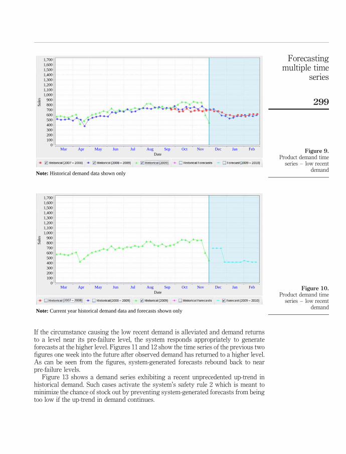
If the circumstance causing the low recent demand is alleviated and demand returnsto a level near its pre-failure level, the system responds appropriately to generateforecasts at the higher level. Figures 11 and 12 show the time series of the previous twofigures one week into the future after observed demand has returned to a higher level.As can be seen from the figures, system-generated forecasts rebound back to nearpre-failure levels.

Figure 13 shows a demand series exhibiting a recent unprecedented up-trend inhistorical demand. Such cases activate the system’s safety rule 2 which is meant tominimize the chance of stock out by preventing system-generated forecasts from beingtoo low if the up-trend in demand continues.


series – low recentdemand

0




100200300400500600700800900

1,000

Sal

es

1,1001,2001,3001,4001,5001,6001,700


series – low recentdemand


DateSep Oct Nov Dec Jan Feb

100


200300400500600700800900

1,000

Sal

es

1,1001,2001,3001,4001,5001,6001,700


series

299

Figure 14 shows the system-generated forecasts for the demand series of Figure 13.As can be seen in the figure, the up-trend is detected and system-generated forecastsfor the first three weeks are adjusted to a level that is as high as the last demand dataobserved.

If the up-trend is broken, the system responds by returning forecasts to morenormal lower levels as can be seen in Figures 15 and 16. Note that the forecasts given inthe latter figure are also subject to safety rule 1, and thus are set at least as high as thefour-week average for the first three weekly forecasts.

Figure 17 shows a demand series exhibiting a recent unprecedented down-trend inhistorical demand. Such cases activate the system’s safety rule 3. This rule minimizes

Figure 11.Product demand timeseries – low recentdemand has returned tousual levels


DateSep Oct Nov Dec Jan MarFeb

100200


300400500600700800900

1,000

Sal

es1,1001,2001,3001,4001,5001,6001,700

Figure 12.Product demand timeseries – low recentdemand has returned tousual levels

0

Date

100200


300400500600700800900

1,000

Sal

es

1,1001,2001,3001,4001,5001,6001,700

Mar Apr May Jun Jul Aug Sep Oct Nov Dec Jan MarFeb

IJICC4,3

300

the chance of stock outs in the presence of a potentially short-lived trend of lowerdemand levels.

Figure 18 shows the system-generated forecasts for the demand series of Figure 17.As can be seen from the figure, the down-trend is detected and system-generatedforecasts for the first three weeks are adjusted to a level that is at least as high as thefour-week average of the most recent historical demand.

If the down-trend is broken, the system responds by returning forecasts to higherlevels near those seen before the down-trend. This is depicted by the demand series andsystem forecasts shown in Figures 19 and 20.

The figures discussed above provide examples of several types of historical demandtime series commonly observed in the live system and show how the system’s


series – up-trend indemand

0

250

500


750

1,000

1,250

1,500

1,750

2,000

2,250

Date

Sal

es

2,500

Mar Apr May Jun Jul Aug Sep Oct Nov Dec Jan Feb


series – up-trend indemand

0

250


500

750

1,000

1,250

1,500

1,750

2,000

2,250

Date

Sal

es

2,500



series

301

three-component model handles these series to produce forecasts that take into accountcurrent demand levels as well as seasonal and “one-off” demand spikes whileminimizing the risk of lost sales revenue due to stock outs resulting from unusualcircumstances such as a power outage or infrastructure failure.

5. Conclusion and future workIn this paper, a real-world forecasting system that automatically models and predictsthousands of time series per week is presented. The system is used by a large fooddistribution company based in Australia to forecast product demand and replenishwarehouse stock for its numerous products distributed out of multiple warehouses

Figure 15.Product demand timeseries – up-trend indemand has broken

0

250

500


750

1,000

1,250

1,500

1,750

2,000

2,250

Date

Sal

es

2,500

Mar Apr May Jun Jul Aug Sep Oct Nov Dec Jan Feb Mar

Figure 16.Product demand timeseries – up-trend indemand has broken

0

250

500


750

1,000

1,250

1,500

1,750

2,000

2,250

Date

Sal

es

2,500


IJICC4,3

302

and services a customer base that covers 91 percent of the combined populations ofAustralia and New Zealand. The total number of demand time series that the systemmust process weekly is on the order of 105.

The system employs a hybrid forecasting model that combines both statistical andheuristic techniques to accurately capture and predict a wide variety of productdemand time series that are influenced by multiple repeating events with minimalcomputation time and without human intervention. A discussion of the algorithm thatunderpins the hybrid model and an analysis of its computational efficiency is provided.System-generated forecasts for several product demand time series taken from the livesystem are presented and discussed.


series – down-trend indemand

0

500400300


200100

800700600

Date

Sal

es

1,7001,6001,5001,4001,3001,2001,1001,000

900



series – down-trend indemand

0


500400300200100

800700600

Date

Sal

es

1,7001,6001,5001,4001,3001,2001,1001,000

900



series

303

The system has been live since November 2009 and has undergone heavy andsustained use since then. The algorithm discussed in this paper has remainedessentially unchanged during this time, and thus has proven to be robust.

One potential direction for future study might be to apply this system to forecastmultiple demand series for other consumer goods such as electronics or insuranceproducts. Another direction to investigate could be to replace the linear regression basemodel with a non-linear model such as a threshold or GARCH model. This kind ofapproach might be able to capture certain non-linear dynamics such as asymmetriccycles or individual outliers that a linear model cannot capture.

Figure 19.Product demand timeseries – down-trend indemand has broken

0

500400300200


100

800700600

Date

Sal

es

1,7001,6001,5001,4001,3001,2001,1001,000

900


Figure 20.Product demand timeseries – down-trend indemand has broken

0

500400300200100


800700600

Date

Sal

es

1,7001,6001,5001,4001,3001,2001,1001,000

900


IJICC4,3

304

Notes

1. These will be cited below.

2. Regression and ARIMA methods can be given a non-linear functional form, however, this isnot common.

3. A Kalman filter is a variation of ARIMA in which the model is expressed in state space form(Makridakis et al. 1998, p. 429).

4. A diffusion model is an ordinary differential equation that is quadratic in the unknownfunction and has constant coefficients (Bass, 1969).

5. A series is stationary if its underlying data-generating process is based on a constant meanand a constant variance (Makridakis et al. 1998, p. 615).

6. After initial analysis it was observed that while some time series exhibited non-stationarityin the mean, none exhibited non-stationarity in the variance.

7. See Makridakis et al. (1998, pp. 324-35) for a detailed discussion of stationarity anddifferencing of time series data.

8. Domain experts in the company confirm that spikes in historical demand occurring duringChristmas and Easter are particularly common in their industry and were able to definespecific time intervals before and after the holiday dates as the representing the relevantholiday season.

9. An example of this is December 25 for years 2007 and 2008: in 2007, it falls on a Tuesday andin 2008 it falls on a Thursday.

10. See Makridakis et al. (1998, pp. 335-47) for a detailed explanation of AR models.

11. See Makridakis et al. (1998, pp. 331-47) for a detailed discussion of seasonal differencing andDiebold (1998, pp. 108-18) for a detailed discussion of seasonal dummy variables and theirusage.

12. See Hamilton (1994, pp. 200-30) for a detailed discussion of parameter estimation for linearregression.

13. In this example, we consider only two years of historical data for clarity.

14. See Knuth (1997) for a detailed discussion of the computational complexity of matrixoperations.

15. Undifferencing is the reverse procedure to differencing. For a second-order differencedseries, the undifferencing must be executed twice.

References

Akgiray, V. (1989), “Conditional heteroskedasticity in time series and stock returns: evidence andforecasts”, Journal of Business, Vol. 62, pp. 55-80.

Araujo, R. (2010), “A quantum-inspired evolutionary hybrid intelligent approach for stockmarket prediction”, International Journal of Intelligent Computing and Cybernetics, Vol. 3,pp. 24-54.

Azadeh, A. and Faiz, Z. (2011), “A meta-heuristic framework for forecasting household electricityconsumption”, Applied Soft Computing, Vol. 11, pp. 614-20.

Back, T. (1996), Evolutionary Algorithms in Theory and Practice: Evolution Strategies,Evolutionary Programming, and Genetic Algorithms, Oxford University Press,New York, NY.


series

305

Baille, R. and Bollerslev, T. (1994), “Cointegration, fractional cointegration, and exchange ratedynamics”, Journal of Finance, Vol. 49, pp. 737-45.

Bass, F. (1969), “A new product growth model for consumer durables”, Management Science,Vol. 15, pp. 215-27.

Bollerslev, T. (1986), “Generalized autoregressive conditional heteroskedasticity”, Journal ofEconometrics, Vol. 31, pp. 307-27.

Chambers, L. (Ed.) (1995), Practical Handbook of Genetic Algorithms: Applications, CRC Press,Boca Raton, FL.

Chen, A. and Leung, M. (2003), “A Bayesian vector error correction model for forecastingexchange rates”, Computers & Operations Research, Vol. 30, pp. 887-900.

Chen, S. and Chen, J. (2010), “Forecasting container throughputs at ports using geneticprogramming”, Expert Systems with Applications, Vol. 37, pp. 2054-8.

Chern, C., Ao, I., Wu, L. and Kung, L. (2010), “Designing a decision-support system fornew product sales forecasting”, Expert Systems with Applications, Vol. 37, pp. 1654-65.

Cheung, Y. and Lai, K. (1993), “A fractional cointegration analysis of purchasing power parity”,Journal of Business and Economic Statistics, Vol. 11, pp. 103-12.

Chiraphadhanakul, S., Dangprasert, P. and Avatchanakorn, V. (1997), “Genetic algorithms inforecasting commercial banks deposit”, Proceedings of the IEEE International Conferenceon Intelligent Processing Systems, Beijing, China, Vol. 1, pp. 557-65.

Clements, M. and Hendry, D. (1995), “Forecasting in cointegrated systems”, Journal of AppliedEconometrics, Vol. 10, pp. 127-46.

Diebold, F. (1998), Elements of Forecasting, International Thomson Publishing, Cincinnati, OH.

Dilip, P. (2010), “Improved forecasting of time series data of real system using geneticprogramming”, GECCO ’10 Proceedings of the 12th Annual Conference on Genetic andEvolutionary Computation, Portland, OR, USA, Vol. 1, pp. 977-8.

Dolgui, A. and Pashkevich, M. (2008), “Extended beta-binomial model for demand forecasting ofmultiple slow-moving inventory items”, International Journal of Systems Science, Vol. 39,pp. 713-26.

Dua, P. and Smyth, D. (1995), “Forecasting home sales using BVAR models and surveydata on households’ buying attitudes for homes”, Journal of Forecasting, Vol. 14,pp. 217-27.

Engle, R. (1982), “Autoregressive conditional heteroskedasticity with estimates of the variance ofUK inflation”, Econometrica, Vol. 50, pp. 987-1008.

Engle, R. and Granger, C. (1987), “Co-integration and error correction: representation, estimation,and testing”, Econometrica, Vol. 55, pp. 251-76.

Fogel, D. and Chellapilla, K. (1998), “Revisiting evolutionary programming”, PSPIEAerosense98. Applications and Science of Computational Intelligence, Vol. 1, pp. 2-11.

Fogel, L., Angeline, P. and Fogel, D. (1995), “An evolutionary programming approach toself-adaptation on finite state machines”, Proceedings of the 4th Annual Conference onEvolutionary Programming, San Diego, CA, USA, Vol. 1, pp. 355-65.

Fogel, L., Owens, A. and Walsh, M. (1966), Artificial Intelligence through Simulated Evolution,Wiley, New York, NY.

Goto, Y., Yukita, K., Mizuno, K. and Ichiyanagi, K. (1999), “Daily peak load forecasting bystructured representation on genetic algorithms for function fitting”, Transactions of theInstitute of Electrical Engineers of Japan, Vol. 119, pp. 735-6.

Gurney, K. (1997), An Introduction to Neural Networks, UCL Press, London.

IJICC4,3

306

Hamilton, J. (1994), Time Series Analysis, Princeton University Press, Princeton, NJ.

He, Z., Huh, S. and Lee, B. (2010), “Dynamic factors and asset pricing”, Journal of Financial andQuantitative Analysis, Vol. 45, pp. 707-37.

Hjalmarsson, E. (2010), “Predicting global stock returns”, Journal of Financial and QuantitativeAnalysis, Vol. 45, pp. 49-80.

Hong, W., Dong, Y., Chen, L. and Wei, S. (2011), “SVR with hybrid chaotic genetic algorithms fortourism demand forecasting”, Applied Soft Computing, Vol. 11, pp. 1881-90.

Johari, D., Rahman, T., Musirin, I. and Aminuddin, N. (2009), “Hybrid meta-EP-ANN techniquefor lightning prediction under Malaysia environment”, AIKED ’09 Proceedings of the8th WSEAS International Conference on Artificial Intelligence, Knowledge Engineeringand Data Bases, Cambridge, UK, Vol. 1, pp. 224-9.

Ju, Y., Kim, C. and Shim, J. (1997), “Genetic based fuzzy models: interest rate forecastingproblem”, Computers & Industrial Engineering, Vol. 33, pp. 561-4.

Kim, D. and Kim, C. (1997), “Forecasting time series with genetic fuzzy predictor ensemble”,IEEE Transactions on Fuzzy Systems, Vol. 5, pp. 523-35.

Knuth, D. (1997), The Art of Computer Programming, Addison-Wesley, Reading, MA.

Lee, Y. and Tong, L. (2011), “Forecasting time series using a methodology based onautoregressive integrated moving average and genetic programming”, Knowledge-BasedSystems, Vol. 24, pp. 66-72.

McMillan, D.G. (2001), “Nonlinear predictability of stock market returns: evidence fromnonparametric and threshold models”, International Review of Economics and Finance,Vol. 10, pp. 353-68.

Makridakis, S., Wheelwright, S. and Hyndman, R. (1998), Forecasting: Methods and Applications,Wiley, New York, NY.

Masih, R. and Masih, A. (1996), “A fractional cointegration approach to empirical tests of PPP:new evidence and methodological implications from an application to the Taiwan/USdollar relationship”, Weltwirtschaftliches Archiv, Vol. 132, pp. 673-93.

Mehdi, K. and Mehdi, B. (2011), “A novel hybridization of artificial neural networks and ARIMAmodels for time series forecasting”, Applied Soft Computing, p. 11.

Michalewicz, Z. (1992), Genetic AlgorithmsþData Structures¼Evolution Programs, Springer,New York, NY.

Mitchell, M. (1996), An Introduction to Genetic Algorithms, MIT Press, Cambridge, MA.

Nasseri, M., Moeini, L. and Tabesh, M. (2011), “Forecasting monthly urban water demandusing extended Kalman filter and genetic programming”, Expert Systems withApplications, p. 38.

Ozden, G., Sayin, S., Woensel, T. and Fransoo, J. (2009), “SKU demand forecasting in the presenceof promotions”, Expert Systems with Applications, Vol. 36, pp. 12340-8.

Ramos, F. (2003), “Forecasts of market shares from VAR and BVAR models: a comparison oftheir accuracy”, International Journal of Forecasting, Vol. 19, pp. 95-110.

Sallehuddin, R. and Shamsuddin, S. (2009), “Hybrid grey relational artificial neural network andauto regressive integrated moving average model for forecasting time-series data”,Applied Artificial Intelligence, Vol. 23, pp. 443-86.

Sarantis, N. (2001), “Nonlinearities, cyclical behaviour and predictability in stock markets:international evidence”, International Journal of Forecasting, Vol. 17, pp. 459-82.


series

307

Sarantis, N. and Stewart, C. (1995), “Structural, VAR and BVAR models of exchange ratedetermination: a comparison of their forecasting performance”, Journal of Forecasting,Vol. 14, pp. 201-15.

Sathyanarayan, R., Birru, S. and Chellapilla, K. (1999), “Evolving nonlinear time series modelsusing evolutionary programming”, CECCO 99: Proceedings of the 1999 Congress onEvolutionary Computation, Washington, DC, USA, Vol. 1, pp. 243-53.

Sayed, H., Gabbar, H. and Miyazaki, S. (2009), “A hybrid statistical genetic-based demandforecasting expert system”, Expert Systems with Applications, Vol. 36, pp. 11662-70.

Shoesmith, G. (1992), “Cointegration, error correction, and improved regional VAR forecasting”,Journal of Forecasting, Vol. 11, pp. 91-109.

Spencer, D. (1993), “Developing a Bayesian vector autoregression forecasting model”,International Journal of Forecasting, Vol. 9, pp. 407-21.

Stock, J. and Watson, M. (2002), “Macroeconomic forecasting using diffusion indexes”,Journal of Business and Economic Statistics, Vol. 20, pp. 147-62.

Theodosiou, M. (2011), “Disaggregation and aggregation of time series components: a hybridforecasting approach using generalized regression neural networks and the theta method”,Neurocomputing, Vol. 20, pp. 896-905.

Tourinho, R. and Neelakanta, P. (2010), “Evolution and forecasting of business-centrictechnoeconomics: a time-series pursuit via digital ecology”, I-Business, Vol. 2, pp. 57-66.

Venkatesan, R. and Kumar, V. (2002), “A genetic algorithms approach to growth phaseforecasting of wireless subscribers”, International Journal of Forecasting, Vol. 18, pp. 625-46.

Wagner, N., Michalewicz, Z., Khouja, M. and McGregor, R. (2007), “Time series forecasting fordynamic environments: the DyFor genetic program model”, IEEE Transactions onEvolutionary Computation, Vol. 11, pp. 433-52.

Wang, F. and Chang, K. (2009), “Modified diffusion model with multiple products using a hybridGA approach”, Expert Systems with Applications, Vol. 36, pp. 12613-20.

Wang, Y., Jiang, W., Yuan, S. and Wang, J. (2008), “Forecasting chaotic time series based onimproved genetic Wnn”, ICNC ’08: Proceedings of the 2008 Fourth InternationalConference on Natural Computation, Jinan, China, Vol. 2008, p. 1.

White, H. (1992), Artificial Neural Networks: Approximation and Learning Theory, Blackwell,Oxford.

Yu, T. and Huarng, K. (2010), “A neural network-based fuzzy time series model to improveforecasting”, Expert Systems with Applications, Vol. 37, pp. 3366-72.

Zou, H., Xia, G., Yang, F. and Wang, H. (2007), “An investigation and comparison of artificialneural network and time series models for Chinese food grain price forecasting”,Neurocomputing, Vol. 70, pp. 2913-23.

About the authors

Neal Wagner is an Assistant Professor of Information Systems at FayettevilleState University, North Carolina, USA and a Scientific Advisor and Consultantfor SolveIT Software – a software company which specializes in supply chainoptimization software for large corporations. His research interests lie inthe field of computational intelligence, particularly in the application ofevolutionary algorithms for modeling, predicting, and optimizing in thepresence of ever-shifting conditions. He has publications in well-knownjournals including IEEE Transactions on Evolutionary Computation,

IJICC4,3

308

Applied Financial Economics, Defence and Peace Economics, and Journal of Business Valuationand Economic Loss Analysis. He holds a PhD in Information Technology and an MS in ComputerScience both from the University of North Carolina at Charlotte, and a BA in Mathematics fromthe University of North Carolina at Asheville. Neal Wagner is the corresponding author and canbe contacted at: [email protected]

Zbigniew Michalewicz is Professor at the University of Adelaide, Australia; alsoat the Institute of Computer Science, Polish Academy of Sciences, Warsaw,Poland, and at the Polish-Japanese Institute of Information Technology,Warsaw, Poland. He also serves as Chairman of the Board for SolveIT Software –a software company which specializes in supply chain optimization software forlarge corporations. He has published over 250 articles and 15 books. Theseinclude How to Solve It: Modern Heuristics, Adaptive Business Intelligence,

as well as Puzzle-based Learning: An Introduction to Critical Thinking, Mathematics, and ProblemSolving, and Winning Credibility: A Guide for Building a Business from Rags to Riches.

Sven Schellenberg is working as Project Manager and Manager for OptimisationApplications at SolveIT Software, an Australian-based company specialising insupply and demand optimisation and predictive modelling. He has an extensivebackground in artificial intelligence and nature inspired optimisation techniquesand their practical application to real-world problems in the fields of scheduling,manufacturing and logistics. He has expert knowledge of applied softwareengineering, software development and project management. His current

research focus is on modelling and optimising of multi-echelon production processes, on whichhe has published several conference papers and book chapters. Sven Schellenberg holds aMaster’s degree in Computer Science from the University of Adelaide with the specialisation onHigh Integrity Software Engineering and Soft Computing, and a Diplom-Ingenieur from theBerufsakademie Berlin/Germany in Computer Science.

Constantin Chiriac is an expert in the development and commercialisation ofsoftware systems, and possesses more than 15 years experience in developingenterprise software applications. He is also the co-author of the groundbreakingbook Adaptive Business Intelligence. Before co-founding SolveIT Software,Constantin worked for the National Bank of Moldova as Project Leader, where heworked on software projects of vital importance for the banking system of theRepublic of Moldova. Later, Constantin worked for several software companies

in the USA, where he used his expertise to develop enterprise software applications that made useof the latest advances in artificial intelligence. These applications were used by numerous global1,000 companies to create measurable improvements in revenue and bottom-line operationalresults. Constantin holds a Master’s degree in Computer Science from the University ofNorth Carolina at Charlotte and a Master’s degree in Economics with a specialisation in Bankingand Stock Exchange Activity from the International Independent University of Moldova.

Arvind Mohais is an expert in optimisation technologies and scientificresearch, and in their application to challenging commercial problems such asmanufacturing, planning, and logistics. He has created novel and uniquealgorithms for these problems, and has wide knowledge of advanced optimisationmethods. With a strong interest in improving profits and efficiency in commercialand industrial areas, he brings more than ten years experience in the


series

309

development, research and application of advanced optimisation and predictive modellingtechnologies. Before joining SolveIT Software, he worked on cutting-edge projects includingthe application of artificial intelligence to classification problems in Earth Science.Arvind Mohais formerly lectured at the University of the West Indies, on subjects includingartificial intelligence, advanced internet technologies, computer algorithms, discrete mathematicsfor computer science and the theory of computation. He holds a PhD in ComputerScience with a specialisation in Particle Swarm Optimisation, a Master’s degree in ComputerScience with a specialisation in Genetic Algorithms, and a Bachelor’s degree in Mathematicsand Computer Science.

IJICC4,3

310

To purchase reprints of this article please e-mail: [email protected] visit our web site for further details: www.emeraldinsight.com/reprints

Documents

IJICC Intelligent techniques for forecasting multiple time ...zbyszek/Papers/p51.pdf · Intelligent techniques for forecasting multiple time series in real-world systems Neal Wagner