IJESM SIGHTINGS ENGINEERINGgnindia.dronacharya.info/Download/Research/DGI_journal... · 2018-02-02 · FROM THE DESK OF EXECUTIVE EDITOR… DearReaders, The qualitative and timely

Approved by

All India Council for Technical Education, New Delhi (India)

Affiliated To:

Dr. A. P. J. Abdul Kalam Technical University, Lucknow (India)

Campus:

# 27, Knowledge Park-III, Greater Noida (U.P.) – 201308 (India)

Phone: 0120-2323854-58, 2322022, Email: advisor.r&[email protected]

Corporate Office:

76P, Part-III, Sector-5, Gurgaon, 122001, Haryana (India)

Phone: 0124-2251602, 2253144, Email: [email protected]

desi

gn: w

ww

.stu

dio1

-indi

a.co

m

IJESM SIGHTINGS INTERNATIONAL JOURNAL OF

ENGINEERINGSCIENCES AND MANAGEMENT

ISSN No. 2231-3273

www.dronacharya.info

A Bi-annual Research Journal of

GREATER NOIDA, U.P., INDIAGROUP OF INSTITUTIONS

J O U R N A L M A S T E R L I S T

Vol. VII | Issue II | Jul-Dec 2017

Brazil 3.5%2.3%

India 60.5%

United States 12.6%

139 different countries have visited this site. 189 flags collected.

1.6%

1.1%

1.0%

1.0%

0.9%

0.8%

0.8%

0.7%

0.7%

0.6%

China

Unknown - A/P

Czech Republic

Iran

Indonesia

Malaysia

Nigeria

Pakistan

United Kingdom

Italy

Egypt

Others 11.9%

ISSN No. 2231-3273

INTERNATIONAL JOURNAL OFENGINEERING SCIENCES AND MANAGEMENT

Vol. VII | Issue II | Jul - Dec 2017

Dr. Kripa Shankar

Professor, IIT Kanpur, India

(Former Vice Chancellor, UPTU)

E-mail: [email protected]

Mr. Rajiv Khoshoo

Senior Vice President

Siemens PLM Software,

California, USA

Email: [email protected]

Mr. Mayank Saxena

Director, Advisory Services

Price Water House Coopers


Dr. T.S. Srivatsan

Professor,

University of Akron, USA


Dr. Kulwant S Pawar

Professor, University of Nottingham, UK


Dr. Roop L. Mahajan

Lewis A. Hester Chair Professor in Engineering

Director, Institute for Critical Technology &

Applied Science (ICTAS) Virginia Tech, Blacksburg, USA


Dr. A.K. Nath

Professor, IIT Kharagpur, India


Dr. Mrinal Mugdh

Associate Vice President,

(Academic Affairs)

University of Houston,

Clear Lake, Texas, USA


Dr. Shubha Laxmi Kher

Director & Associate Professor,

Arkansas State University, USA


PATRON

Dr. SatishYadav

ChairmanDronacharya Group of Institutions, Greater Noida

EDITOR-IN-CHIEF

Dr. Ashish Soti

DirectorDronacharya Group of Institutions, Greater NoidaE-mail: [email protected]

EXECUTIVE EDITOR

Wg Cdr (Prof) TPN Singh

Advisor (Research & Development)Dronacharya Group of Institutions, Greater NoidaE-mail: advisor.r&[email protected]

EDITORIAL BOARD

Dr. Ganesh Natarajan

Founder - 5F WorldChairman - NASSCOM Foundation & Global Talent TrackPresident - HBS Club of IndiaE-mail: [email protected]

Dr. Satya Pilla

Boeing Space Exploration,iGET Enterprises,Embry-Riddle Aeronautical UniversityE-mail: [email protected]

Dr. R.P. Mohanty

Former Vice ChancellorShiksha 'O' Anusandhan UniversityBhubaneswar, IndiaEmail: [email protected]

Mr. Uday Shankar Akella

Chairman & Managing DirectorRSG Information Systems Pvt LtdHyderabad, IndiaEmail: [email protected]

Dr. Sanjay Kumar

Vice ChancellorITM University ChhatishgarhFormer Principal AdvisorDefence Avionics Research Establishment (DARE)E-mail: [email protected]

BUT WE CAN BUILD OUR YOUTH FOR THE FUTURE

WE CAN NOT ALWAYS BUILD THE FUTURE FOR OUR YOUTH,

GROUP OF INSTITUTIONS

-Franklin D Roosevelt

Here We Build Your Future

B. TECH COURSES| |Computer Science & Engineering Electronics & Communication Engineering Electronics & Computer Engineering

Electrical & Electronics Engineering Mechanical Engineering Computer Science and Information Technology| |

Information Technology Civil Engineering|

POST GRADUATE COURSESMaster of Business Administration (MBA) Master of Computer Application (MCA)|

Campus: #27, Knowledge Park- III, Greater Noida (UP) Phone: 0120-2323851-58, 2322022 | Email: [email protected] India Council for Technical Education, New Delhi (India) Dr. A. P. J. Abdul Kalam Technical University, Lucknow (India)Approved by: | Affiliated To:

DRONACHARYA GROUP OF INSTITUTIONS


DRONACHARYAGROUP OF INSTITUTIONSGREATER NOIDA, U.P., INDIA

INTERNATIONAL JOURNAL OFENGINEERING SCIENCESAND MANAGEMENT

ISSN No. 2231-3273

Volume VII | Issue II | Jul - Dec 2017

INTERNATIONAL JOURNAL OF

ENGINEERING, SCIENCES AND MANAGEMENT

All rights reserved: International Journal of Engineering, Sciences and Management,takes no responsibility for accuracy of layouts and diagrams.These are schematic or concept plans..

Editorial Information:For details please write to the Executive Editor, International Journal of Engineering, Sciences and Management, DronacharyaGroup of Institutions, # 27, Knowledge Park-III, Greater Noida – 201308 (U.P.), India.

Telephones:Landline: +91-120-2323854, 2323855, 2323856, 2323857, 2323858

+91-120-2322022Mobile: +91-8826006878

Telefax:+91-120-2323853

E-mail:advisor.r&[email protected]@[email protected]

Website:www.dronacharya.infowww.ijesm.in

The Institute does not take any responsibility about the authenticity and originality of the material contained in thisjournal and the views of the authors although all submitted manuscripts are reviewedbyexpert.

ISSN No. 2231-3273Int. J. Engg. Sc. & Mgmt. Vol. VII | Issue II | Jul - Dec 2017

ISSN No. 2231-3273

ADVISORY BOARDMEMBERS

Prof. (Dr.) Raman Menon UnnikrishnanCollege of Engineering and Computer Science

Professor of Electrical and Computer Engineering

California State University Fullerton, Fullerton,

CA 92831


Mr. Sanjay BajpaiScientist-G, Department of Science & Technology

Ministry of Science & Technology

New Delhi, India


Prof. (Dr.) Prasad K D V YarlagaddaQueensland University of Technology

South Brisbane Area, Australia.


Prof. (Dr.) Devdas KakatiFormer Vice Chancellor, Dibrugarh University

Former Professor, IIT-Madras


Prof. (Dr.) Pradeep K KhoslaChancellor, University of California

San Diego

[email protected]

Prof. (Dr.) S G DeshmukhDirector

Indian Institute of Information Technology &

Management (IIITM), Gwalior

Email: [email protected].

Mr. S. K. LalwaniHead (Projects)

Consultancy Development Centre (CDC)

DSIR, Ministry of Science & Technology

Government of India


Dr. Shailendra PalviaProfessor of Management Information Systems

Long Island University, USA

Email: [email protected], [email protected]

Prof. (Dr.) Vijay VaradharajanMicrosoft Chair in Innovation in Computing

Macquaire University, NSW 2109, Australia.


Prof. (Dr.) Surendra S YadavDept. of Management Studies

IIT Delhi, India


Int. J. Engg. Sc. & Mgmt. Vol. VII | Issue II | Jul - Dec 2017

FROM THE DESK OF

EXECUTIVE EDITOR…

Dear Readers,

The qualitative and timely publication of Vol. VII / Issue-II (Jul–Dec 2017) of our esteemed International Journal of

Engineering, Sciences and Management (ISSN: 2231-3273) has brought great joy and happiness to the entire fraternity of the

journal and honorable members of the Editorial and Advisory Board. The board members rich experience and varied expertize is

providing immense succour in propelling the journal to attain an envious position in areas of research and development and

accentuate its visibility. The distinctive feature is indexing of the journal by Jour Informatics, Index Copernicus, Google Scholar

and DOAJ. It is a matter of great pride and honor that the journal has been viewed by researchers from one hundred and thirty nine

countries across the globe. The aim of journal is to percolate knowledge in various research fields and elevate high end research.

The objective is being pursued vigorously by providing the necessary eco-system for research and development.

Large number of research papers were received from all over the globe for publication and we thank each one of the

authors personally for soliciting the journal. We also extend our heartfelt thanks to the reviewers and members of the editorial

board who so carefully perused the papers and carried out justified evaluation. Based on their evaluation, we could accept twelve

research papers for this issue across the disciplines. We are certain that these papers will provide qualitative information and

thoughtful ideas to our accomplished readers. We thank all the readers profusely who conveyed their appreciation on the quality

and content of the journal and expressed their best wishes for future issues. We convey our deep gratitude to the Editorial Board,

Advisory Board and all office bearers who have made possible the publication of this journal in the planned time frame.

We invite all the authors and their professional colleagues to submit their research papers for consideration for

publication in our forthcoming issue i.e. Vol. VIII | Issue I | Jan–Jun 2018 as per the “Scope and Guidelines toAuthors” given at the

end of this issue.Any comments and observations for the improvement of the journal are most welcome.

We wish all readers meaningful and quality time while going through the journal.

Wg Cdr (Prof) TPN SinghExecutive Editor

International journal of Engineering, Sciences and Management (IJESM)A bi-annual Research journal of Dronacharya Group of Institutions,

Greater Noida, UP, India.

Dec 2017


EFFECTS OF BIODIESEL ON ENGINE PERFORMANCE AND TAILPIPE CHARACTERISTICSDaniel Argueta, Haowei Wang1

LUCENEX: A SEARCH ENGINE FOR XML DATA ON TOP OF APACHE LUCENEWeimin He, Teng Lv, Ping Yan, Aaron Salisbury10

MONGRELIZED ALGORITHMS FOR REAL POWER LOSS MINIMIZATIONK. Lenin18

ANALYSIS OF BOOST CONVERTER USING DIFFERENT PID TUNINGTECHNIQUES COMPARED WITH CLOSE LOOP SYSTEMKiran H. Raut

50

30 A MODEL FOR FACE RECOGNITION SYSTEM USING VOILA-JONES ALGORITHMPriyadarshini Jainapur, Sowmyashree

38 DESIGN, ESTIMATION AND COSTING OF SEWAGE TREATMENT PLANT: A CASE STUDYAdarsh S, Shesha Prakash M N, Tejas S Pinaki, Darshan Paul

Amit L. Meshram, Sagar D. Shelare, Machchhendra K. Sonpimple

DESIGN AND DEVELOPMENT OF CONSTANT PRESSURE DELIVERING PUMP59

DESIGN AND DEVELOPMENT OF DROP WEIGHT GENERATOR FOR HARNESSINGGREEN ENERGYMahesh K, Lithesh J, Sujith A

69

103 SCOPE AND GUIDELINES FOR AUTHORS

14 UWB SLOT ANTENNA FOR BODY AREA NETWORK (BAN)Sanjay Kumar, Saurabh Shukla

EMPLOYEE ENGAGEMENT: EMPIRICAL EVIDENCE ON RECENT REPORTSDr.G. Swetha, D. Pradeep Kumar77

COMPARISON OF EXISTING AND PREDICTED SOLID WASTE MANAGEMENTIN AN URBAN AREAAdarsh S, Shesha Prakash M N, Aishwarya M and Roshan

94

COST EFFECTIVENESS IN QUALITY CONSTRUCTIONP.G.Seetharam86


1

ABSTRACT

1. INTRODUCTION

EFFECTS OF BIODIESEL ON ENGINE PERFORMANCE AND TAILPIPE

CHARACTERISTICS

Daniel Argueta

Mechanical Engineering Department

California State University Fullerton, Fullerton, CA 92831, USA

Haowei Wang*

Mechanical Engineering Department

California State University Fullerton, Fullerton, CA 92831, USA

Tel: +1-657-278-7913


*Corresponding author

This paper presents the findings of the effects of biodiesels B5, B20, and B99 on engine performance and tailpipe

characteristics in comparison to Diesel #2. A single cylinder diesel engine with a dynamometer and a portable gas analyzer

are used for experiments. Thermal efficiency, emissions of CO2, NOx, CO, HC are measured at a wide range of engine

speeds from 1000 rpm to 2500 rpm and at three loads of 4.32 Nm, 6.48 Nm, and 8.64 Nm. The results show that the

biofuels tested affect the engine efficiency and tailpipe characteristics differently at different loads.

Keywords: Biodiesel, Efficiency, Tailpipe Characteristics.

In an effort to abide by growing governmental demands steps are being taken to create alternate fuels in order to

reduce the use of limited fossil fuels. By the year 2022 the Unites States Department of Energy’s Renewable Fuel Standard

(RFS) dictates that 36 billion gallons of renewable fuel be blended into transportation fuels [1]. Such fuels, particularly ones

deemed renewable, need to be high in energy density and emit fewer greenhouse gases than would a typical petroleum

based fossil fuel. Such a fuel must be compatible with internal combustions engines found in transportation vehicles as

transportation is such a major consumer of fossil fuel. One such alternative to conventional fossil fuels is biodiesel.

Biodiesel is a renewable energy source that is also biodegradable [1], making it an attractive alternative to fossil fuels, even

to petroleum based diesel. Biodiesel is often made from vegetable oils, such as corn or animal fats that undergo a

transesterification process and produce alkyl esters [2]. Since these biodiesels are derived from plant matter the carbon

emissions they release can be absorbed by crops also used to produce biofuel, thus creating a possibly carbon neutral life

cycle. It is also considered an Advanced Biofuel and a Biomass-Based Diesel, meaning that is a renewable fuel source made

from feedstocks and reduces Green House Gas emission in its lifecycle by at least 50% [1].

mailto:[email protected]

2

Biodiesels, namely ethanol derived from corn or sugarcane, have been studied [3]. However other blends of biodiesel have

yet to be examined namely biodiesels that use biofuel derived from non-edible oils. Such biodiesels must be compatible

with preexisting diesel engines, or at the very least require minimal alterations. It is for this reason some fuels are over

looked as they require changes to an engine in order for proper combustion to occur. Such fuels must have high cetane

numbers to limit ignition delay and low viscosities to avoid build up in the engine. Biodiesels have generally comparable

cetane values along similar energy densities and heat of vaporization, when compared to petroleum based diesel [4]. With

the idea that a renewable fuel would be used for transportation in mind, it is important to study the emissions and

performance of the test fuels through a basic diesel internal combustion engine.

Monitoring the emissions of varied blends of biodiesel is imperative. The combustion of a biodiesel blend will emit carbon

dioxide CO2, unburned hydrocarbons (HC), carbon monoxide CO, NOx emissions, and particulate matter (PM). The overall

usefulness of a biodiesel most not only burn cleaner than petroleum based fuels, but also carry enough energy to be a

suitable transportation fuel, and thus deliver similar energy outputs.

The fuels tested included, Diesel #2, B5, B20, and B99. Diesel #2, B5, and B20 were obtained from Propel and

B99 was obtained from Downs Energy Fuel and Lubricants. Diesel #2, B5, and B20 has a fuel density of 740 as well

as a calorific value of 43.8 B99 has a density of 740 however its calorific value is 37.4. In this regard,

the amount of biofuel found in the fuel has little effect on its density and calorific value.

In order to test the various fuels, a Modified 4 Stroke Diesel Engine TD212 from TecQuipment was used. The

engine has a max power and torque output of 3.75 kW and 10.8 Nm respectively, at 3000 rpm. The compression ratio is

22:1 with a 232cc capacity. The engine is attached to a dynamometer and has a volumetric fuel gauge. An engine cycle

analysis software and Enerac portable gas analyzer are installed. The exhaust system has a thermocouple installed to

measure exhaust gas temperatures. A Kistler pressure sensor is installed, to measure the cylinder head pressure of the

engine.

Table 1: Engine specifications

An encoded is attached from the dynamometer to the Data Acquisition (DAQ) system. This DAQ system is

equipped with a computer GUI and a data analysis software. The software directly measures the engine parameters: engine

speed in rpm, engine torque in Nm, engine power in W, ambient air temperature in ˚C, exhaust gas temperature in ˚C,

differential pressure in the engine’s intake system in Pa. The parameters calculated include heat of combustion, air mass

flow rate, fuel mass flow rate, and thermal efficiency. Theses parameters help to examine the performance of the Biodiesels

tested.

2. EXPERIMENTAL METHOD

Engine type Equipment (TD212)

Fuel Injection System Direct

Max Power (Kw) 3.75

Compression Ratio 22:1

Number of Cylinders 1

Number of Cycles 4

Intake system Naturally Aspirated

Cooling system Air cooled

Engine Capacity (CC) 232

3

To measure the actual emissions of each of the fuels, the Enerac portable emission analyzer system was connected to the

tailpipe. The system recorded , , CO, , and HC concentrations that are created during combustion. The Enerac

can measure oxide from 0- 25%, from 0-5000 ppm, and uses a non-dispersive infrared gas sensor to measure CO

from 0-15%, , from 0-20%, and HC from 0-30000 ppm.

The fuels were tested at four different speeds, evenly incremented in 500 rpm intervals from 1000-2500 rpm. Each fuel was

tested at 3 different target loads 4.32, 6.48, and 8.64Nm. Each load case was tested with the given rpm range and interval.

First the engine was brought to the sampling rpm with the specified target load via the dynamometer. At each incremental

step, the engine performance parameters were recorded for 2 minutes under steady state conditions. Here steady state is

determined by monitoring the exhaust gas temperatures. Steady State is reached when the exhaust gas temperatures

converge to a single temperature or to changes of less than 1% per minute. Emissions were collected after steady state was

reached and were collected for 10 minutes. At the end of the data collection periods, the data was averaged over 2 minutes

for performance data and 10 minutes for emissions data.

3.1 Thermal Efficiency Looking at the thermal efficiency data in Figures 1-3, it is seen that B20 has an efficiency

between 60% and 80% for all three loads over the entire tested rpm spectrum. B5 tends to decline in efficiency as rpm

increases from all load cases. B99 has comparable efficiencies to both B5 and B20, however for 4.32 Nm and 6.48 Nm

loads, there is a near 20% drop in efficiency around 1500 rpm. The regular petroleum based Diesel #2 holds similar trends

for all load cases and similar characteristics over the rpm range. In general, the efficiency of Diesel #2 is below that of B20

and B99.

Figure 1: Efficiency of various fuels with 4.32Nm load

B5 and Diesel #2 behave most similarly in terms of thermal efficiency at all conditions studied. This is likely due to the fact

that B5 has the least amount of Biofuel and is most similar to the petroleum based diesel #2.

3. RESULTS AND DISCUSSION

4


B99 has the greatest efficiency when engine speed is above 2000 rpm at all three loads. B5’s efficiency drops quickly as the

rpm increases. Its close counterpart Diesel #2 has similar characteristics.


In all accounts, biofuel increases the efficiency of diesel. The efficiency of Diesel #2 is below all other test fuels. This

indicates that biodiesels can and do have higher efficiency ratings than regular petroleum based diesels, particularly Diesel

#2. To this end however in can be seen that B99 has high efficiency at above 2500rpm.

4. CONCLUSION

5

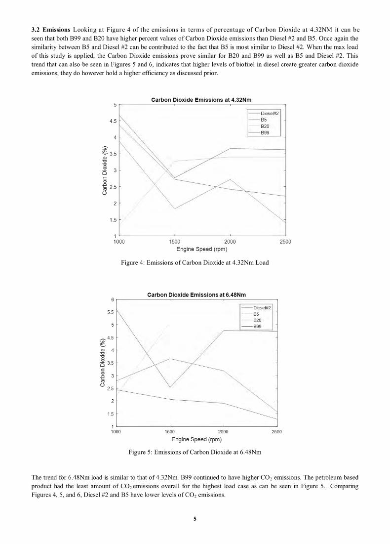
3.2 Emissions Looking at Figure 4 of the emissions in terms of percentage of Carbon Dioxide at 4.32NM it can be

seen that both B99 and B20 have higher percent values of Carbon Dioxide emissions than Diesel #2 and B5. Once again the

similarity between B5 and Diesel #2 can be contributed to the fact that B5 is most similar to Diesel #2. When the max load

of this study is applied, the Carbon Dioxide emissions prove similar for B20 and B99 as well as B5 and Diesel #2. This

trend that can also be seen in Figures 5 and 6, indicates that higher levels of biofuel in diesel create greater carbon dioxide

emissions, they do however hold a higher efficiency as discussed prior.

Figure 4: Emissions of Carbon Dioxide at 4.32Nm Load

Figure 5: Emissions of Carbon Dioxide at 6.48Nm

The trend for 6.48Nm load is similar to that of 4.32Nm. B99 continued to have higher CO2 emissions. The petroleum based

product had the least amount of CO2 emissions overall for the highest load case as can be seen in Figure 5. Comparing

Figures 4, 5, and 6, Diesel #2 and B5 have lower levels of CO2 emissions.

6

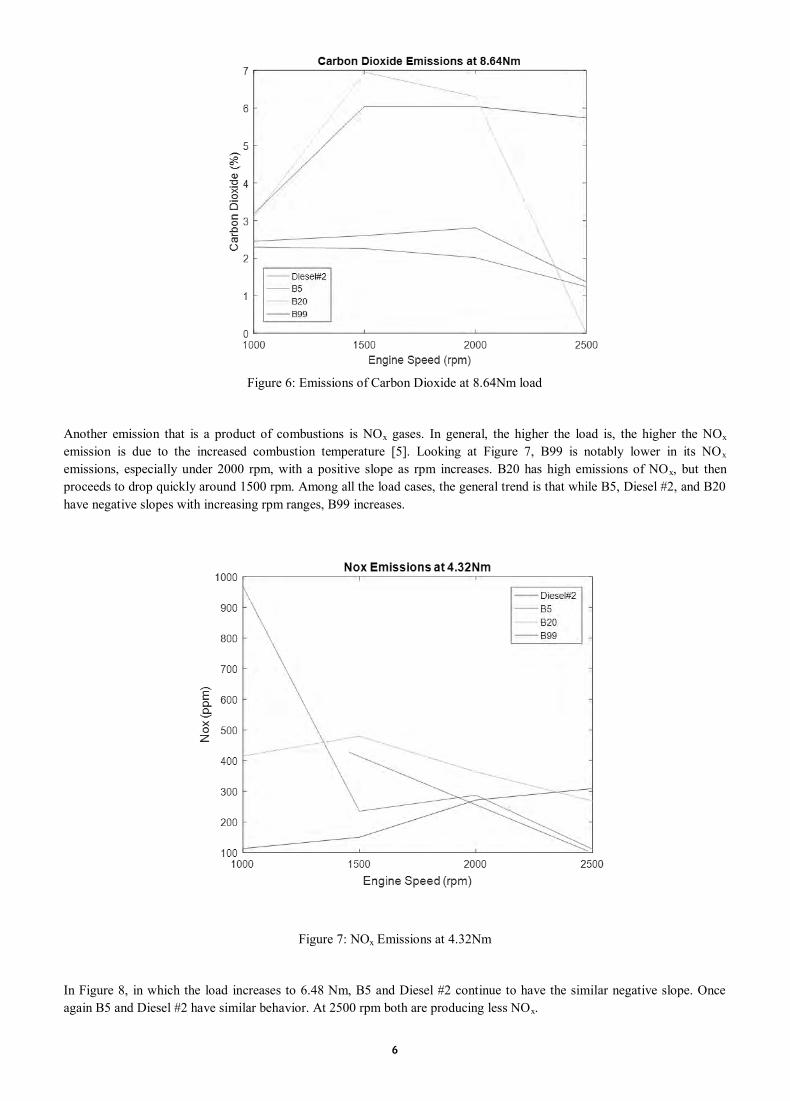
Figure 6: Emissions of Carbon Dioxide at 8.64Nm load

Another emission that is a product of combustions is NOx gases. In general, the higher the load is, the higher the NOx

emission is due to the increased combustion temperature [5]. Looking at Figure 7, B99 is notably lower in its NOx

emissions, especially under 2000 rpm, with a positive slope as rpm increases. B20 has high emissions of NOx, but then

proceeds to drop quickly around 1500 rpm. Among all the load cases, the general trend is that while B5, Diesel #2, and B20

have negative slopes with increasing rpm ranges, B99 increases.

Figure 7: NOx Emissions at 4.32Nm

In Figure 8, in which the load increases to 6.48 Nm, B5 and Diesel #2 continue to have the similar negative slope. Once

again B5 and Diesel #2 have similar behavior. At 2500 rpm both are producing less NOx.

7

Figure 8: Emission of NOx gases at 6.48Nm

In Figure 9 in which the load increases to 8.64 Nm, once again B5 and Diesel #2 have a lower emission rating. B99 ends at

2500 rpm with just under 700 ppm. Overall B5 and Diesel #2 have lower emission trends as opposed to B99 and B20 which

appear to increase emission concentration with increases in rpm

Figure 9: Emission of NOx gases at 8.64Nm.

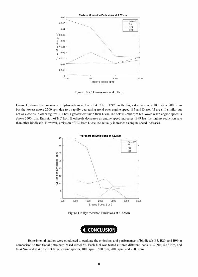
Figure 10 presents the CO emissions from all fuels studied at load of 4.32 Nm. The carbon monoxide emissions are lower

than that of NOx. B5 and Diesel #2 have similar trends again. B99 continued to have higher amounts of emissions but it

decreases as engine speed increases.

8

Figure 10: CO emissions as 4.32Nm

Figure 11 shows the emission of Hydrocarbons at load of 4.32 Nm. B99 has the highest emission of HC below 2000 rpm

but the lowest above 2500 rpm due to a rapidly decreasing trend over engine speed. B5 and Diesel #2 are still similar but

not as close as in other figures. B5 has a greater emission than Diesel #2 below 2500 rpm but lower when engine speed is

above 2500 rpm. Emission of HC from Biodiesels decreases as engine speed increases. B99 has the highest reduction rate

than other biodiesels. However, emission of HC from Diesel #2 actually increases as engine speed increases.

Figure 11: Hydrocarbon Emissions at 4.32Nm

Experimental studies were conducted to evaluate the emissions and performance of biodiesels B5, B20, and B99 in

comparison to traditional petroleum based diesel #2. Each fuel was tested at three different loads, 4.32 Nm, 6.48 Nm, and

8.64 Nm, and at 4 different target engine speeds, 1000 rpm, 1500 rpm, 2000 rpm, and 2500 rpm.

4. CONCLUSION

9

The results indicate that varied levels of biofuel do in fact affect not only the efficiency of the engine it is burning in, but the

emissions as well. Generally, the amount of biodiesel in the fuel blends positively affects the thermal efficiency of the

engine, especially when the engine speed is above 1500 rpm at all loads studied. B99 has the highest thermal efficiency

when the engine speed is above 2000 rpm.

The emissions of the test fuels varied greatly but generally the content of biodiesel tents to increase of emission of CO2, CO,

and HC. The effects of biodiesel on the emission of NOx varies greatly for the biodiesels studied here at different engine

loads and engine speeds.

In summary, for the fuels studied here, biodiesels tend to increase the thermal efficiency of an engine but also increase the

emissions of CO2, CO and HC.

1. U.S Department of Energy, Alternative Fuels Data Center, 7 February 2017. [Online]. Available:

http://www.afdc.energy.gov/laws/RFS.

2. Pinto, Angelo C., et al. Biodiesel: an overview, Journal of the Brazilian Chemical Society 16(6B), 2005, p. 1313-

1330.

3. B. E. D. Seungdo Kim, Life cycle assessment of various cropping systems utilized for producing biofuels:

Bioethanol and biodiesel, 29(6), 2005, p. 427-439.

4. Agarwal, Avinash Kumar. Biofuels (alcohols and biodiesel) applications as fuels for internal combustion engines,

Progress in energy and combustion science, 33(3), 2007, p. 233-271.

5. Yilmaz, Nadir, Erol Ileri, and Alpaslan Atmanli. Performance of biodiesel/higher alcohols blends in a diesel

engine, International Journal of Energy Research 40(8), 2016, p. 1134-1143.

REFERENCES

http://www.afdc.energy.gov/laws/RFS

10

ABSTRACT

1. INTRODUCTION

LUCENEX: A SEARCH ENGINE FOR XML DATA ON TOP OF APACHE LUCENE

Weimin He*

Department of Computing and New Media Technologies

University of Wisconsin-Stevens Point, 2100 Main Street

Stevens Point, WI, 54481, USA



Teng Lv School of Information Engineering

Anhui Xinhua University

Hefei, China

Ping Yan School of Science

Anhui Agricultural University

Hefei, China

Aaron Salisbury

Department of Computing and New Media Technologies

University of Wisconsin-Stevens Point

Stevens Point, USA

In this research paper, we have developed a prototype system termed LuceneX that serves as a search engine for

XML data across a directory containing XML documents. Our search engine was built on top of Apache Lucene, which is a

high-performance, simple text based search engine library written entirely in Java. We utilized Windows Forms in .NET

framework to design and implement the graphical user interface of LuceneX. In order to embed Java code into .NET

application, we leveraged IKVM.NET to convert our Java code into .NET DLL files.

Keywords: XML, Search Engine, Apache Lucene

As we know, XML has become the standard form for representing and exchanging data on the web, there is an

increasing interest in indexing, querying, and ranking text-centric XML documents. XML query languages, such as XPath

[13] and XQuery [14], were very powerful in expressing exact queries over XML data, but they did not meet the needs of

the IR community since they were lacking of full-text capabilities.

11

In order to support full-text search functionalities over XML documents, we built a XML search engine called LuceneX,

that supports a variety of XML full-text search queries over XML data. Our search engine was built on top of Apache

Lucene[5], which is a high-performance, simple text based search engine library.

The rest of the paper is organized as follows: Section 2 introduces Apache Lucene and IKVM.NET, which are the back-

ends of our search engine, LuceneX. Section 3 presents our search engine LuceneX in more details, including architecture,

GUI design, and type of queries supported. Section 4 discusses related work. Finally, section 5 concludes the paper and

presents the future work.

2.1 Apache Lucene Our XML search engine was built on top of Apache Lucene[5], which is a high-performance,

scalable, full-featured text search engine library written entirely in Java. Apache Lucene is a technology suitable for

applications that requires full-text search, and it is supported by the Apache Software Foundation and is released under the

Apache Software License. Lucene offers some powerful full-text search features such as high-performance indexing,

ranked searching, different query types(phrase queries, wildcard queries, proximity queries, range queries), fielded

searching, and so on.

2.2 IKVM.NET IKVM.NET is an implementation of Java for Mono[16] and the Microsoft .NET Framework[17]. It

includes the following components[15]:

A Java Virtual Machine implemented in .NET

A .NET implementation of the Java class libraries

Tools that enable Java and .NET interoperability

In order to embed Java code into our .NET Windows Forms applications, we leveraged IKVM.NET to convert our Java

code into .NET DLL files. IKVM.NET includes ikvmc, a Java bytecode to .NET IL translator. We run the following

command to convert the Java library to .NET dll files: ikvmc -target:library mylib.jar to create mylib.dll.

In order to support full-text search of XML document collections, we have developed a prototype system termed

LuceneX that serves as a search engine for XML data across a directory containing XML documents. Our search engine

was built on top of Apache Lucene, which is a high-performance, simple text based search engine library written entirely in

Java. We utilized Windows Forms in .NET framework to design and implement the graphical user interface of LuceneX. In

order to embed Java code into .NET application, we leveraged IKVM.NET to convert our Java code into .NET DLL files.

Our system allows the user to specify a directory of XML documents to create an in-memory index. Then the user may pose

a query, with a built-in syntax assist feature, against the index that was created. The query result is a list of XML document

hits, each of which can be viewed as a raw document as well as a stylized HTML document. Any well-formed XML

document can be styled dynamically, regardless of structure, thanks to a combination of SAX and XSLT technologies built

on top of Lucene. The snap shot of LuceneX is shown in the following figure.

2. APACHE LUCENE AND IKVM.NET

3. LUCENEX

12

Currently, the types of queries supported by LuceneX include simple keyword, keyword intersection, document title, range

of document titles, document date range, and proximity of keywords to each other. In addition to this base functionality, it

has been expanded to make XML specific searching possible using LINQ to XML. Here tag (element) names can be

searched on, as well by a tag’s value equaling or not equaling something.

Since XML is the data format for a wide variety of web data repositories, extensive work has been motivated on

designing powerful query languages, developing efficient indexing and query evaluation algorithms, and proposing

effective ranking schemes over XML data[1, 2, 4, 18,6, 8]. The related work can be classified into three categories.

Approaches in the first category are focused on extending existing complex XML query languages, such as XQuery, with

IR search predicates and incorporating simple IR scoring methods into the query evaluation. Khalifa et al[1] proposes bulk

algebra called TIX, which integrates simple IR scoring schemes into a traditional pipelined query evaluator for an XML

database. More specifically, new operators and efficient access methods are proposed to generate and manipulate scores of

XML fragments during query evaluation. TeXQuery[2] supports a powerful set of fully composable full-text search

primitives, which can be seamlessly integrated into the XQuery language. It mostly focuses on the TeXQuery language

design and the underlying formal model, but also provides a costing model[9]. Strategies in the second category are

dedicated to extending traditional IR models for scoring simple XPath-like queries with full-text extension. In [3], the

authors present a framework that relaxes a full-text XPath query by dropping some predicates from its closure and scoring

the approximate answers using predicate penalties. They further propose novel scoring methods by extending TF*IDF

ranking to account for both structure and content while considering query relaxations[4]. Sigurbjornsson et al,[10] propose

a framework that decomposes the query into several path-term pairs, evaluates these pairs separately and produces a final

ranking that takes into account the scores of different sources of evidence. In the third category, efforts are made to address

the problem of efficiently producing ranked results for keyword search queries over XML documents. XRank[7] extends

Google-like keyword search to XML. The authors propose an algorithm for scoring XML elements that takes into account

both hyperlink and containment edges. New inverted list index structures based on Dewey IDs and associated query

processing algorithms are also presented. XSEarch[6] is a semantic search engine that extends simple keyword search by

incorporating keyword context information into the query, i.e., each query term is a keyword-label pair instead of a single

keyword. XSEarch extends the TF*IDF ranking scheme to rank the results. Another work, XKSearch[11], introduces the

concept of smallest lowest common ancestors (SLCAs) and proposes two efficient algorithms,

4. RELATED WORK

13

Indexed Lookup Eager and Scan Eager, for keyword search in XML documents according to the SLCA semantics. Note

that all the above proposals consider querying and ranking original XML documents, and returning XML fragments as

query answers.

In this paper, we have developed a full-text search engine on top of Apache Lucene. Our search engine can support

a wide range of XML full-text search queries over a collection of XML documents. As our future work, we plan to test our

system over a large collection of XML documents in real world. We also plan to develop a ranking scheme which can rank

the returned XML documents based on TF*IDF model in IR community.

1. S. Al-Khalifa, C. Yu, and H. V. Jagadish, Querying Structured Text in an XML Database," in Proceedings of

SIGMOD'03, 2003.

2. S. Amer-Yahia, C. Botev, and S. Shanmugasundaram, TeXQuery: A Full-Text Search Extension to XQuery," in

Proceedings of WWW'04, 2004.

3. S. Amer-Yahia, L. V.S. Lakshmanan, and S. Pandit, FleXPath: Flexible Structure and Full-Text Querying for

XML," in Proceedings of SIGMOD'04, 2004.

4. S. Amer-Yahia, N. Koudas, A. Marian, D. Srivastava, and D. Toman Structure and Content Scoring for XML," in

Proceedings of VLDB'05, 2005.

5. Lucene. http://lucene.apache.org/

6. S. Cohen, J. Mamou, Y. Kanza, and Y. Sagiv, XSEarch: A Semantic Search Engine for XML," in Proceedings of

VLDB'03, 2003.

7. L. Guo, F. Shao, C. Botev, and J. Shanmugasundaram, XRANK: Ranked Keyword Search over XML Documents,"

in Proceedings of SIGMOD'03, 2003.

8. L. Chen, and Y. PapakonstantinouL, Supporting Top-K Keyword Search in XML Databases," in Proceedings of

ICDE'10, 2010.

9. A. Marian, S. Amer-Yahia, N. Koudas, and D. Srivastava, Adaptive Processing of Top-K Queries in XML," in

Proceedings of ICDE'05, 2005.

10. B. Sigurbjornsson, J. Kamps, and M. D. Rijke, Processing Content-Oriented XPath Queries," in Proceedings of

CIKM'04, 2004.

11. Y. Xu and Y. Papakonstantinou. Efficient Keyword Search for Smallest LCAs in XML Databases. SIGMOD 2005.

12. R. B. Yates and B. R. Neto, Modern Information Retrieval, ACM Press,1999.

13. 13, XML Path Language (XPath) 2.0. http://www.w3.org/TR/xpath20/

14. XQuery 1.0: An XML Query Language. http://www.w3.org/TR/xquery/

15. IKVM.NET. https://www.ikvm.net/

16. Mono. http://www.mono-project.com/

17. Microsoft .NET Framework. https://www.microsoft.com/net/download/framework

5. CONCLUSION

REFERENCES

14

ABSTRACT

1. INTRODUCTION

UWB SLOT ANTENNA FOR BODY AREA NETWORK (BAN)

Sanjay Kumar* ITM University

3rd Floor , Shyam Plaza, Pandri, Raipur-492001(C.G)

Tel. No.0771-6640438

[email protected]


Saurabh Shukla

Defence Avionics Research Establishment (DARE)

Kaggadasapura Main Road,

C V Raman Nagar, Bangalore-560093

Tel.No. 080-25047699

[email protected]

An UWB slot antenna has been designed and developed for BAN purpose. It is a compact, low profile and light

weight antenna which can be used for on-body communication link. Slot antenna consists of a slot in ground plane and a

stub attached with 50Ω feed. The proposed antenna covers 4-10 GHz frequency range antenna with a moderate gain of 4

dB. The antenna has been designed and fabricated on a low cost FR-4 substrate to reduce the cost and physical dimensions

of the antenna.

Keywords: Ultra Wide Band (UWB), Slot Antenna, Body Area Network (BAN) and On-Body Communication.

Ultra-Wideband (UWB) is defined as a frequency band covering 3.1 GHz to 10.6 GHz. It is a wide bandwidth

technology for short range ultra-high speed communications. UWB transmissions represent a bandwidth of at least 500

MHz, as well as bandwidth of at least 20% of the centre frequency. It also offers a bit rate greater than 100 Mbps within a

10-meter radius for wireless communications. The advantages of UWB include low-power transmission, robustness for

multi-path fading and low power dissipation.

Printed planar monopole antennas are widely used for UWB communications because they offer wide frequency impedance

bandwidth and omnidirectional radiation patterns. Moreover simple structure, easy fabrication on printed circuit boards

(PCBs), easy integration with other components and low cost are some additional features of these antennas.


15

The other proven topology for UWB antennas is slot antennas. In UWB slot antenna design, a large slot is cut in the ground

plane to achieve a high level of electromagnetic coupling with the tuning stub. The wide-slot antenna offers wide

impedance bandwidth but its operating bandwidth is limited by the degradation of the radiation patterns at higher

frequencies [1]. The coupling is thus dependent on the type and shape of stub and slot. The coupling actually controls the

impedance matching. In order to optimize the coupling between the microstrip line and the tapered slot, different stub

shapes have been studied and reported in literature. Some of the commonly used stub shapes are shown in Fig. 1. For

elliptical and circular shape tuning stubs, the impedance matching is very poor due to poor electromagnetic coupling

between the feed-line and tapered slot. The rectangular shape tuning stub shows a good coupling with tapered shape slot

proving a wider impedance matching for UWB application.

Fig. 1 Different stub geometry

The proposed UWB antenna has dimensions of 16mm 16mm 1.64mm and it is designed on FR-4

substrate having = 4.4 and loss tangent 0.02. It consists of a tapered slot in the ground plane of dimensions 13mm

7mm with an arc of 1mm radius. On the other side of the substrate, 50Ω feed line is designed and terminated with a

rectangular stub of dimensions 7.5mm 3mm. The offset between the stub and ground plane plays an important role and

its optimized value is 1.65mm [2]. The simulated structure and surface current on antenna are shown in Fig. 2 and Fig. 3

respectively.

Fig. 2 Antenna Geometry

Fig. 3 Surface Current

2. DESIGN PARAMETERS

16

The spacing and arc radius of proposed antenna are taken as parameters to study their impact on antenna performance. The

antenna has been simulated and optimized with these parameters to achieve desired bandwidth and radiation characteristics.

The optimized return loss of proposed antenna is presented in Fig.4. The results suggest that 10 dB return loss has been

achieved for over 3.6-11.6 GHz frequency range[3][4].

Fig. 4 Simulated S11 in dB

The simulated radiation pattern of the simulated antenna has been presented in Fig. 5. It is clear from the simulated

result that the antenna radiates in broadside direction and the radiation pattern doesn’t have nulls in the upper and lower

hemisphere which is required for wireless applications.

Fig. 5 Simulated radiation pattern

The simulated gain of the antenna over the 3-11 GHz frequency range is presented in Fig. 6.The plot suggests that

the antenna offers moderate gain ranging 3-5 dB over 4-11GHz.

Fig. 6 Simulated Gain (dB)

3. PARAMETRIC STUDY

17

The final values of the antenna parameters are given in Table1 for reference.

Table -1: Design Parameters

From the simulated results it can be concluded that introduction of the tapered slot instead of the rectangular slot

changes the electric field distribution and as a result, the impedance matching is much improved resulting in overall

enhancement of operating bandwidth. It is also observed that performance can also be improved by employing tapered slot

structure with a rectangular tuning stub. This combination produces wider bandwidth than with a circular, elliptical, and

square-shaped slot.

The wireless sensor nodes in BAN are designed to be as small as possible hence the requirements for the antenna system

are very crucial in terms of physical dimensions. Most of the BAN antennas are electrically small and the aim of a designer

is to find out the best possible compromise between antenna dimensions and radiation characteristics.

The antenna presented in this paper is very small and can be integrated with modern MMIC based Transmit-Receive

modules for BAN. Also the antenna fulfills other requirements of wearable antennas like light weight, low cost and low

profile.

As an extension of this work, the same antenna can be kept with human body model to study SAR. It can be optimized to

achieve more bandwidth and improved performance under the presence of human body.

The authors would like to thank Director, DARE and Chancellor ITM University for his continuous support and

encouragement for this work. All the designs and simulations were carried out using CST Microwave Studio available at

DARE, Bangalore.

1. Liu, Y. F., Lan, K. L., Xue, Q., Chan, C. H. Experimental Studies of Printed Wide-slot Antenna for Wide-band

Applications. IEEE Antennas & Wireless Propagation Letters, 3, 273 – 275 (2004).

2. Dastranj, A., Imani, A., Moghaddasi, M. N. Printed Wide-slot Antenna for wideband applications. IEEE

Transactions on Antennas & Propagation, 56, 3097 – 3102 (2008).

3. Jan, J. Y., Kao, J. C. Novel Printed Wide-Band Rhombus-like Slot Antenna with an Offset Microstrip-fed Line.

IEEE Antennas & Wireless Propagation Letters, 6, 249 – 251 (2007).

4. Jan, J. Y., Su, J. W. Bandwidth Enhancement of a Printed Wide-slot Antenna with a Rotated Slot. IEEE

Transactions on Antennas & Propagation, 53, 2111 – 2114 (2005).

5. CST Microwave Studio, User’s Manual 2011

4. CONCLUSION

5. ACKNOWLEDGEMENTS

REFERENCES

Parameter Name Optimized value

Substrate Length 16mm

Substrate Length 16mm

Slot Length 13mm

Slot Width 7mm

Gap between stub and Slot 1.65mm

Stub Length 7.5mm

Stub Width 3mm

18

ABSTRACT

1. INTRODUCTION

MONGRELIZED ALGORITHMS FOR REAL POWER LOSS MINIMIZATION

K. Lenin Professor

Prasad V. Potluri Siddhartha Institute of Technology

Kanuru, Vijayawada, Andhra Pradesh -520007

Email : [email protected]

In this paper Chaotic Local Search Artificial Bee Colony algorithm (CLABC) algorithm & Augmented Particle Swarm

optimization (APSO) algorithm are used to solve optimal reactive power problem. Artificial Bee Colony algorithm is a

global optimization algorithm which is motivated by the foraging behaviour of honey bee swarms. Basic Artificial Bee

Colony algorithm (ABC) has the advantages of strong robustness, fast convergence and high flexibility, fewer setting

parameters, but it has the disadvantages premature convergence in the later search period and the accuracy of the optimal

value which cannot meet the requirements sometimes. The premature convergence issue in Artificial Bee Colony algorithm

has been improved by increasing the number of scout and rational using of the global optimal value and by chaotic local

Search. The Chaotic local Search ABC (CLABC) algorithm used to solve the reactive power dispatch problem. Particle

swarm optimization (PSO) has received increasing interest from the optimization community due to its simplicity in

implementation and its inexpensive computational overhead. However, PSO has premature convergence, especially in

complex multimodal functions. Extremal Optimization is a recently developed local-search heuristic method and has been

successfully applied to a wide variety of hard optimization problems. To overcome the limitation of PSO, this paper

proposes a novel hybrid algorithm, called Augmented Particle Swarm optimization algorithm (APSO), through introducing

extremal optimization into PSO. The hybrid approach elegantly combines the exploration ability of PSO with the

exploitation ability of Extreme optimization. Both the projected algorithms CLABC & APSO has been tested in standard

IEEE 57,118 bus test systems and simulation results show clearly the enhanced performance of the both projected

algorithms in tumbling the real power loss. But CLABC has slight edge over the APSO in reducing the real power loss.

Keywords: Chaotic Local Search Artificial Bee Colony algorithm, Augmented Particle Swarm optimization optimization,

optimal reactive power, Transmission loss.

Different algorithms are utilized to solve the Reactive Power Dispatch problem. Different types of numerical techniques

like the gradient method [1-2], Newton method [3] and linear programming [4-7] have been already used to solve the

optimal reactive power dispatch problem. The voltage stability problem play’s an important role in power system planning

and operation [8].Evolutionary algorithms such as genetic algorithm, Hybrid differential evolution algorithm, Biogeography

Based algorithm, a fuzzy based approach, an improved evolutionary programming [9-15] have been already utilized to solve

the reactive power flow problem In [16-18] different methodologies like interior point, upgraded approach are successfully

handled the optimal power problem. In [19-20], a programming based approach and probabilistic algorithm is used to solve

the optimal reactive power dispatch problem. ABC (Artificial Bee Colony) algorithm is based on the intelligent behavior of


19

honeybee swarms finding nectar and sharing the information of food sources with each other [21-27]. ABC algorithm has

the advantages of strong robustness, fast convergence and high flexibility, fewer control parameters. The premature

convergence issue of the Artificial Bee Colony algorithm has been improved by increasing the number of scout and rational

using of the global optimal value and chaotic local Search. The Chaotic local Search ABC (CLABC) algorithm used to

solve the reactive power dispatch problem and it has been tested in standard test systems. Particle Swarm Optimization

(PSO) algorithm is a recent addition to the list of global search methods. This derivative-free method is particularly suited

to continuous variable problems and has received increasing attention in the optimization community. PSO is inspired by

the paradigm of birds flocking. PSO consists of a swarm of particles and each particle flies through the multi-dimensional

search space with a velocity, which is constantly updated by the particle's previous best performance and by the previous

best performance of the particle's neighbours. PSO can be easily implemented and is computationally inexpensive in terms

of both memory requirements and CPU speed [28]. Recently, a general-purpose local-search heuristic algorithm named

Extremal Optimization (EO) has been proposed by Boettcher and Percus [29, 30]. To avoid premature convergence of PSO,

an idea of combining PSO with EO is addressed in this paper called as Augmented Particle Swarm optimization (APSO)

algorithm and it has been tested in standard test systems. Both the projected algorithms CLABC & APSO has been tested in

standard IEEE 57,118 bus test systems and simulation results show clearly the enhanced performance of the both projected

algorithms in tumbling the real power loss. But CLABC has slight edge over the APSO in reducing the real power loss.

Active power loss

Main aim of the reactive power dispatch problem is to reduce the active power loss in the transmission network, which can

be described as:

(1)

Where gk: is the conductance of branch between nodes i and j, Nbr: is the total number of transmission lines in power

systems.

Voltage profile improvement

For minimization of the voltage deviation in PQ buses, the objective function turns into:

(2)

Where ωv: is a weighting factor of voltage deviation.

VD is the voltage deviation given by:

(3)

Equality Constraint

The equality constraint of the Reactive power problem is represented by the power balance equation, and can be written as,

where the total power generation must cover the total power demand and total power loss:

(4)

Where, -Total Power Generation, -Total Power Demand, – Total Power Loss.

Inequality Constraints

Inequality constraints define the limitations in power system components and power system security.

Upper and lower bounds on the active power of slack bus, and reactive power of generators are written as follows:

(5)

(6)

Upper and lower bounds on the bus voltage magnitudes are described as follows:

(7)

Upper and lower bounds on the transformers tap ratios are given as follows:

(8)

2. OBJECTIVE FUNCTION

20

Upper and lower bounds on the compensators reactive powers are written as follows:

(9)

Where N is the total number of buses, NT is the total number of Transformers; Nc is the total number of shunt reactive

compensators.

Artificial Bee Colony (ABC) contains three groups: employed bee, onlooker bee and scout. The bee going to the food

source which is visited by it previously is employed bee. The bee waiting on the dance area for making decision to choose a

food source is onlooker bee. The bee carrying out random search is scout bee. The onlooker bee with scout also called

unemployed bee. In the ABC algorithm, the collective intelligence searching model of artificial bee colony consists of three

essential components: employed, unemployed foraging bees, and food sources. The employed and unemployed bees search

for the rich food sources, which close to the bee's hive. The employed bees store the food source information and share the

information with onlooker bees. The number of employed bees is equal to the number of food sources and also equal to the

amount of onlooker bees. Employed bees whose solutions cannot be improved through a predetermined number of trials,

specified by the user of the ABC algorithm and called “limit”, become scouts and their solutions are abandoned.

3.1. The Procedure of ABC

The classical ABC includes four main phases.

Initialization Phase: The food sources, whose population size is SN, are randomly generated by scout bees. The number of

Artificial Bee is NP. Each food source xm is a vector to the optimization problem, xm has D variables and D is the

dimension of searching space of the objective function to be optimized. The initiation food sources are randomly produced

via the expression (10).

(10)

where ui and li are the upper and lower bound of the solution space of objective function, rand(0,1) is a random number

within the range [0,1].

Employed Bee Phase: A employed bee flies to a food source and finds a new food source within the neighborhood of the

food source. The higher quantity food source will be selected. The food source information stored by employed bee will be

shared with onlooker bees. A neighbor food source vmi is determined and calculated by the following equation (11).

(11)

where xk is a randomly selected food source, i is a randomly chosen parameter index, is a random number within the

range [-1,1]. The range of this parameter can make an appropriate adjustment on specific issues. The fitness of food source

is essential in order to find the global optimal. The fitness is calculated by the following formula (12). After that a greedy

selection is applied between xm and vm.

= (12)

where fm(xm) is the objective function value of xm.

Onlooker Bee Phase: Onlooker bees observe the waggle dance in the dance area and calculate the profitability of food

sources, then randomly select a higher food source. After that onlooker bees carry out randomly search in the neighborhood

of food source. The quantity of a food source is evaluated by its profitability and the profitability of all food sources. Pm is

determined by the formula

(13)

where fitm(xm) is the fitness of xm.

Onlooker bees search the neighborhood of food source according to the expression (14)

(14)

3. ARTIFICIAL BEE COLONY ALGORITHM

21

Scout Phase: If the profitability of food source cannot be improved and the times of unchanged greater than the

predetermined number of trials, which called "limit" and specified by the user of the ABC algorithm, the solutions will be

abandoned by scout bees. Then, the scouts start to randomly search the new solutions. If solution xi has been abandoned,

the new solution xm will be discovered by the scout. The xm is defined by expression (15)

(15)

Where is the new generated food source, rand (0,1) is a random number within the range [0,1], u i and li are the upper

and lower bound of the solution space of objective function.

In the basic Artificial Bee Colony algorithm, the best solution founded by onlooker bee which adopted the local search

strategy is unable to reach the ideal level of accuracy. In order to improve the accuracy of optimal solution and obtain the

fine convergence ability, we use the chaotic search method to solve this problem. In the Chaotic local Search ABC

algorithm, onlooker bees apply chaotic sequence to enhance the local searching behavior and avoid being trapped into local

optimum. In onlooker bee phase, chaotic sequence is mapped into the food source. Onlooker bees make a decision between

the old food source and the new food source according to a greedy selection strategy. In this paper, the well-known logistic

map which exhibits the sensitive dependence on initial conditions is employed to generate the chaotic sequence. The chaos

system used in this paper is defined by

(16)

(17)

Where x is the new food source and xi is the chaotic variable, R is the radius of new food source being generated. The food

source xmi is in the central of searching region. After the food source has been generated, onlooker bee will exploit the new

food source and select the higher profitable one using a greedy selection.

Chaotic search method includes the following steps:

Step1. Setting the iterations (cycle parameter) of chaotic search and produce a vector =. , which is the

initial value of chaotic search.

Step2. The chaotic sequence is generated according to expression (16) and a new food source, which combining the chaotic

sequence with the original food source, is obtained following the equation (17).

Step3. Calculating the profitability of the new food source and using the greedy selection select the higher profitability food

source.

Step4. If the number of chaotic search iterations greater than maximum, the artificial bee algorithm will enter the scout bee

phase, or else enter the next chaotic search iteration.

4.1. Global Search Strategy In the basic Artificial Bee Colony algorithm only one scout, but we added another one

into the modified Artificial Bee Colony algorithm in order to improve the global convergence ability. When a scout bee find

the food source unchanged times greater than the limit parameter, it will produce a new food source and replace the

original one .Scout bee discover the new food source using the best optimal value strategy which accelerate the global

convergence rate. Assume that the solution xi has been abandoned and the scout bee will generate the new solution xm using

the following equation

(18)

(i) (19)

Where xm is new food source produced by scout bee using the global optimal value xbest and is a random number

within the range [-1,1].

4. CHAOTIC LOCAL SEARCH ABC

22

4.2 The Procedure of CLABC

The procedure of CLABC is as following:

Initial Phase

According to equation (10) discovering the initial food sources Itertime = 1;

While (Itertime <= MaxCycle)

Employed Bee Phase

Step1. According to expression (11) searching the neighbourhood food source;

Step2. Calculate the function value;

Step3. According to formula (12) evaluate fitness of the food sources.

Onlooker Bee Phase

Step1. According to expression (13) calculate the profitability;

Step2. Onlooker bee in the guide of equation (14) and (15) exploiting the local optimal solution;

Step3. Calculating the function value of new food source;

Step4. Evaluating new food source fitness according to equation (15).

Scout Bee Phase

if (trial>limit)

Step1. The first scout randomly discovering the new food source;

Step2 The second scout bee updating the food source, which hit the limit parameter, according to formula (18) and (19).

Search the global optimal value

Global Min

End while

PSO is a population based optimization tool, where the system is initialized with a population of random particles and the

algorithm searches for optima by updating generations. Suppose that the search space is D-dimensional. The position of the

i-th particle can be represented by a D-dimensional vector and the velocity of this particle is

.The best previously visited position of the i-th particle is represented

by and the global best position of the swarm found so far is denoted by . . The fitness of each

particle can be evaluated through putting its position into a designated objective function. The particle's velocity and its new

position are updated as follows:

(20)

(21)

Where N is the population size, the superscript t denotes the iteration number, is

the inertia weight, r1 and r2 are two random values in the range [0,1], c1 and c2 are the cognitive and social scaling

parameters which are positive constants.

5. PARTICLE SWARM OPTIMIZATION

23

EO is inspired by recent progress in understanding far-from-equilibrium phenomena in terms of self-organized criticality, a

concept introduced to describe emergent complexity in physical systems. EO successively updates extremely undesirable

variables of a single sub-optimal solution, assigning them new, and random values. Moreover, any change in the fitness

value of a variable engenders a change in the fitness values of its neighbouring variable.

Procedure of EO algorithm.

1. Randomly generate algorithm. Set the optimal solution and the minimum cost

function .

2. For the current solution X ,

a. Evaluate the fitness for each variable , ,

b. Rank all the fitness and find the variable, with lowest fitness i.e. for all i.

c. Choose one solution in the neighbourhood X, such that j-th variable must change its state.

d. Accept X= unconditionally

e. If < then set and

3. Repeat set 2 as long as desired

4. Return and

Note that in the EO algorithm, each variable in the current solution X is considered “species”. In this study, we adopt the

term “component” to represent “species” which is usually used in biology. For example, if X = (x1, x2, x3), then x1, x2 and x3

are called “components” of X . From the EO algorithm, it can be seen that unlike genetic algorithms which work with a

population of candidate solutions, EO evolves a single sub-optimal solution X and makes local modification to the worst

component of X . A fitness value ¸i is required for each variable xi in the problem, in each iteration variables are ranked

according to the value of their fitness. This differs from holistic approaches such as evolutionary algorithms that assign

equal-fitness to all components of a solution based on their collective evaluation against an objective function.

Note that PSO has great global-search ability, while EO has strong local-search capability. In this work, we propose an

Augmented PSO algorithm (APSO) which combines the merits of PSO and EO. This hybrid approach makes full use of the

exploration ability of PSO and the exploitation ability of EO. Consequently, through introducing EO to PSO, the proposed

approach may overcome the limitation of PSO and have capability of escaping from local optima. In the main procedure of

Augmented PSO algorithm, the fitness of each particle is evaluated through putting its position into the objective function.

However, in the EO procedure, in order to find out the worst component, each component of a solution should be assigned a

fitness value. We defined the fitness of each component of a solution for an unconstrained minimization problem as

follows. For the i-th particle, the fitness of the k-th component is defined as the mutation cost, i.e. OBJ(Xik) - OBJ(Pg),

where X ik is the new position of the i-th particle obtained by performing mutation only on the k-th component and leaving

all other components fixed, OBJ(Xik) is the objective value of X ik, and OBJ(Pg) is the objective value of the best position in

the swarm found so far.

6. EXTREMAL OPTIMIZATION (EO)

7. AUGMENTED PSO ALGORITHM

24

EO algorithm for the RPO problem

1. Set the index of the current particle i =1.

2. for the position of the i-th particle

a. perform mutation on each component of Xi

One by one, while keeping other components fixed. Then D new positions can be obtained;

b. evaluate the fitness OBJ(Xik) - OBJ(Pg) of each component Xik , k

c. compare all the components according to their fitness values and find out the worst adapted component xiw ,and

then xiw is the new position corresponding to xiw ,w.

d. if OBJ(xiw)< OBJ(xi) then set Xi=Xiw , and OBJ(xi) = OBJ(xiw)continue the next step. Otherwise, Xi keeps

unchanged and go to Step 3;

e. update pi and pg

3. If i equals to the population size N , return the results; otherwise, set i = i +1 and go to Step 2.

APSO Algorithm for solving reactive power dispatch problem.

1. Initialize a swarm of particles with random positions and velocities N on D dimensions.

Set iteration = 0.

2. Evaluate the fitness value of each particle, and update.

3. Update the velocity and position of each particle using Eq.11 and Eq.12, respectively.

4. Evaluate the fitness value of each particle, and update.

5. If (iteration mod INV) =0, the EO procedure is introduced. Otherwise, continue the next step.

6. If the terminal condition is satisfied, go to next step; otherwise, set iteration = iteration +1, and go to Step 3.

7. Output the optimal solution and the optimal objective function value.

Proposed Chaotic Local Search Artificial Bee Colony algorithm (CLABC) algorithm & Augmented Particle Swarm

optimization (APSO) algorithm has been tested in standard IEEE-57 bus power system. The reactive power compensation

buses are 18, 25 and 53. Bus 2, 3, 6, 8, 9 and 12 are PV buses and bus 1 is selected as slack-bus. The system variable limits

are given in Table 1.

The preliminary conditions for the IEEE-57 bus power system are given as follows:

Pload = 12.213 p.u. Qload = 3.024 p.u.

The total initial generations and power losses are obtained as follows:

=12.4642 p.u. = 3.3011 p.u.

Ploss = 0.25729 p.u. Qloss = -1.2028 p.u.

Table 2 & 3 shows the various system control variables i.e. generator bus voltages, shunt capacitances and transformer tap

settings obtained after optimization which are within the acceptable limits. In Table 4, shows the comparison of optimum

results obtained from proposed methods with other optimization techniques. These results indicate the robustness of

proposed approaches for providing better optimal solution in case of IEEE-57 bus system. But CLABC has slight edge over

the APSO in reducing the real power loss.

8. SIMULATION RESULTS

25

Table 1. Variable limits

Table 2. Control variables obtained after optimization

Reactive Power Generation Limits Bus no 1 2 3 6 8 9 12 Qgmin -1.4 -.015 -.02 -0.04 -1.3 -0.03 -0.4 Qgmax 1 0.3 0.4 0.21 1 0.04 1.50

Voltage And Tap Setting Limits

vgmin Vgmax vpqmin Vpqmax tkmin tkmax

0.9 1.0 0.91 1.05 0.9 1.0

Shunt Capacitor Limits

Bus no 18 25 53

Qcmin 0 0 0 Qcmax 10 5.2 6.1

Control Variables

CLABC

V1 1.1

V2 1.041

V3 1.049

V6 1.037

V8 1.030

V9 1.011

V12 1.020

Qc18 0.0670

Qc25 0.200

Qc53 0.0465

T4-18 1.010

T21-20 1.059

T24-25 0.872

T24-26 0.880

T7-29 1.061

T34-32 0.881

T11-41 1.024

T15-45 1.040

T14-46 0.910

T10-51 1.020

T13-49 1.060

T11-43 0.910

T40-56 0.900

T39-57 0.950

T9-55 0.950

26

Table 3. Control variables obtained after optimization

Table 4. Comparison results

Control Variables APSO V1 1.1

V2 1.037

V3 1.032 V6 1.049

V8 1.041

V9 1.010

V12 1.020

Qc18 0.0651

Qc25 0.200

Qc53 0.0470 T4-18 1.010

T21-20 1.072 T24-25 0.891

T24-26 0.897 T7-29 1.077

T34-32 0.891 T11-41 1.031

T15-45 1.040 T14-46 0.910

T10-51 1.021 T13-49 1.060

T11-43 0.910 T40-56 0.900

T39-57 0.950 T9-55 0.950

S.No. Optimization Algorithm Finest Solution Poorest Solution Normal Solution

1 NLP [31] 0.25902 0.30854 0.27858 2 CGA [31] 0.25244 0.27507 0.26293

3 AGA [31] 0.24564 0.26671 0.25127 4 PSO-w [31] 0.24270 0.26152 0.24725

5 PSO-cf [31] 0.24280 0.26032 0.24698 6 CLPSO [31] 0.24515 0.24780 0.24673

7 SPSO-07 [31] 0.24430 0.25457 0.24752 8 L-DE [31] 0.27812 0.41909 0.33177

9 L-SACP-DE [31] 0.27915 0.36978 0.31032 10 L-SaDE [31] 0.24267 0.24391 0.24311

11 SOA [31] 0.24265 0.24280 0.24270 12 LM [32] 0.2484 0.2922 0.2641

13 MBEP1 [32] 0.2474 0.2848 0.2643 14 MBEP2 [32] 0.2482 0.283 0.2592

15 BES100 [32] 0.2438 0.263 0.2541 16 BES200 [32] 0.3417 0.2486 0.2443

17 Proposed CLABC 0.22098 0.23129 0.22114 18 Proposed APSO 0.22110 0.23134 0.22127

27

Then Chaotic Local Search Artificial Bee Colony algorithm (CLABC) algorithm & Augmented Particle Swarm

optimization (APSO) algorithm has been tested in standard IEEE 118-bus test system [33] .The system has 54 generator

buses, 64 load buses, 186 branches and 9 of them are with the tap setting transformers. The limits of voltage on generator

buses are 0.95 -1.1 per-unit., and on load buses are 0.95 -1.05 per-unit. The limit of transformer rate is 0.9 -1.1, with the

changes step of 0.025. The limitations of reactive power source are listed in Table 5, with the change in step of 0.01.

Table 5. Limitation of reactive power sources

The statistical comparison results of 50 trial runs have been list in Table 6 and the results clearly show the better

performance of proposed Chaotic Local Search Artificial Bee Colony algorithm (CLABC) algorithm & Augmented Particle

Swarm optimization (APSO) algorithm. But CLABC has slight edge over the APSO in reducing the real power loss.

Table 6. Comparison results

In this paper Chaotic Local Search Artificial Bee Colony algorithm (CLABC) algorithm & Augmented Particle Swarm

optimization (APSO) algorithm have been successfully solved the Reactive power optimization problem. The performance

of the proposed algorithms demonstrated through its evaluation in IEEE 57,118 test bus systems & from the simulation

study it has been found that both the proposed algorithms efficiently reduces the real power loss when compared to other

standard reported algorithms. But CLABC has slight edge over the APSO in reducing the real power loss.

1. O.Alsac,and B. Scott, “Optimal load flow with steady state security”,IEEE Transaction. PAS -1973, pp. 745-751.

2. Lee K Y ,Paru Y M , Oritz J L –A united approach to optimal real and reactive power dispatch , IEEE

Transactions on power Apparatus and systems 1985: PAS-104 : 1147-1153

3. A.Monticelli , M .V.F Pereira ,and S. Granville , “Security constrained optimal power flow with post contingency

corrective rescheduling” , IEEE Transactions on Power Systems :PWRS-2, No. 1, pp.175-182.,1987.

4. Deeb N ,Shahidehpur S.M ,Linear reactive power optimization in a large power network using the decomposition

approach. IEEE Transactions on power system 1990: 5(2) : 428-435

5. E. Hobson ,’Network consrained reactive power control using linear programming, ‘ IEEE Transactions on power

systems PAS -99 (4) ,pp 868=877, 1980

9. CONCLUSION

REFERENCES

BUS 5 34 37 44 45 46 48

QCMAX 0 14 0 10 10 10 15

QCMIN -40 0 -25 0 0 0 0

BUS 74 79 82 83 105 107 110

QCMAX 12 20 20 10 20 6 6

QCMIN 0 0 0 0 0 0 0

Active power

loss (MW) BBO [34]

ILSBBO/ strategy1

[34]

ILSBBO/ strategy1

[34]

Proposed CLABC

Proposed APSO

Min 128.77 126.98 124.78 117.91 118.81

Max 132.64 137.34 132.39 121.90 122.07

Average 130.21 130.37 129.22 119.06 120.98

28

6. K.Y Lee ,Y.M Park , and J.L Oritz, “Fuel –cost optimization for both real and reactive power dispatches” , IEE

Proc; 131C,(3), pp.85-93.

7. M.K. Mangoli, and K.Y. Lee, “Optimal real and reactive power control using linear programming” , Electr.Power

Syst.Res, Vol.26, pp.1-10,1993.

8. C.A. Canizares , A.C.Z.de Souza and V.H. Quintana , “ Comparison of performance indices for detection of

proximity to voltage collapse ,’’ vol. 11. no.3 , pp.1441-1450, Aug 1996 .

9. S. Sakthivel, M. Gayathri, V. Manimozhi, “A Nature Inspired Optimization Algorithm for Reactive Power Control

in a Power System”, International Journal of Recent Technology and Engineering (IJRTE) ,pp29-33 Volume-2,

Issue-1, March 2013.

10. D. Devaraj, and B. Yeganarayana, “Genetic algorithm based optimal power flow for security enhancement”, IEE

proc-Generation.Transmission and. Distribution; 152, 6 November 2005.

11. A. Berizzi, C. Bovo, M. Merlo, and M. Delfanti, “A ga approach to compare orpf objective functions including

secondary voltage regulation,” Electric Power Systems Research, vol. 84, no. 1, pp. 187 – 194, 2012.

12. C.-F. Yang, G. G. Lai, C.-H. Lee, C.-T. Su, and G. W. Chang, “Optimal setting of reactive compensation devices

with an improved voltage stability index for voltage stability enhancement,” International Journal of Electrical

Power and Energy Systems, vol. 37, no. 1, pp. 50 – 57, 2012.

13. P. Roy, S. Ghoshal, and S. Thakur, “Optimal var control for improvements in voltage profiles and for real power

loss minimization using biogeography based optimization,” International Journal of Electrical Power and Energy

Systems, vol. 43, no. 1, pp. 830 – 838, 2012.

14. B. Venkatesh, G. Sadasivam, and M. Khan, “A new optimal reactive power scheduling method for loss

minimization and voltage stability margin maximization using successive multi-objective fuzzy lp technique,”

IEEE Transactions on Power Systems, vol. 15, no. 2, pp. 844 – 851, may 2000.

15. W. Yan, S. Lu, and D. Yu, “A novel optimal reactive power dispatch method based on an improved hybrid

evolutionary programming technique,” IEEE Transactions on Power Systems, vol. 19, no. 2, pp. 913 – 918, may

2004.

16. W. Yan, F. Liu, C. Chung, and K. Wong, “A hybrid genetic algorithminterior point method for optimal reactive

power flow,” IEEE Transactions on Power Systems, vol. 21, no. 3, pp. 1163 –1169, aug. 2006.

17. J. Yu, W. Yan, W. Li, C. Chung, and K. Wong, “An unfixed piecewiseoptimal reactive power-flow model and its

algorithm for ac-dc systems,” IEEE Transactions on Power Systems, vol. 23, no. 1, pp. 170 –176, feb. 2008.

18. F. Capitanescu, “Assessing reactive power reserves with respect to operating constraints and voltage stability,”

IEEE Transactions on Power Systems, vol. 26, no. 4, pp. 2224–2234, nov. 2011.

19. Z. Hu, X. Wang, and G. Taylor, “Stochastic optimal reactive power dispatch: Formulation and solution method,”

International Journal of Electrical Power and Energy Systems, vol. 32, no. 6, pp. 615 – 621, 2010.

20. A. Kargarian, M. Raoofat, and M. Mohammadi, “Probabilistic reactive power procurement in hybrid electricity

markets with uncertain loads,” Electric Power Systems Research, vol. 82, no. 1, pp. 68 – 80, 2012.

21. Zhou Xi-xiang,Li Jia-sheng,Yang Sai-liang, “The Digital PID Parameter Tuning Based on Chaos Particle Swarm

Optimization”, Power Electronics,44(10):62-64, 2010.

22. Anan Banharnsakun,Tiranee Achalakul,Booncharoen Sirinaovakul, “The best-so-far selection in the Bee Clony

algorithm”, Applied Computing, 11,2888-2901, 2011.

23. Fei Kang, Junjie Li, Zhenyue Ma , Rosenbrock, “artificial bee colony algorithm for accurate global optimization of

numerical functions”, Information Sciences: S0020-0255(11)00198-8, DOI: 10.1016/j.ins.2011.04.024,2011.

24. Mustafa Sonmez ,”Artificial Bee Colony algorithm for optimization of truss structures”, Applied Soft Computing

11(2011)2406-2018,2011

25. O.Altinoz Tolga, A.Egemen Yilmaz, Gerhard Wilhelm Weber, “Chaos Particle Swarm Optimized PID Controller

for the Inverted Pendulum System”, second International Conference on Engineering Optimization, September 6-

9,2010,Lisbon ,Portugal, 2010.

29

26. Tatjana Davidovic´, Duˇsan Ramljak, MilicaˇSelmic´, Duˇsan Teodorovic´, “Bee colony optimization for the p-

center problem”, Computers & Operations Research, 38(2011)1367-1376,2011.

27. Ioná Maghali Santos de Oliveira , Roberto Schirru, “Swarm intelligence of artificial bees applied to In-Core Fuel

Management Optimization”, Annals of Nuclear Energy 38(2011)1039-1045,2011.

28. R.C. Eberhart, J. Kennedy, “A New Optimizer Using Particle Swarm Theory”, Proceedings of theSixth

International Symposium on Micro machine and Human Science, Nagoya, Japan, 1995, pp.39-43.

29. S. Boettcher, A. G. Percus, “Extremal optimization: methods derived from co-evolution”, Proceedings of the

genetic and evolutionary computation conference,1999, pp. 825-832.

30. S. Boettcher, A. G. Percus, “Nature's way of optimizing”, Artificial Intelligence 119(2000)275-286.

31. Chaohua Dai, Weirong Chen, Yunfang Zhu, and Xuexia Zhang, “Seeker optimization algorithm for optimal

reactive power dispatch,” IEEE Trans. Power Systems, Vol. 24, No. 3, August 2009, pp. 1218-1231.

32. J. R. Gomes and 0. R. Saavedra, “Optimal reactive power dispatch using evolutionary computation: Extended

algorithms,” IEE Proc.-Gener. Transm. Distrib.. Vol. 146, No. 6. Nov. 1999.

33. IEEE, “The IEEE 30-bus test system and the IEEE 118-test system”, (1993), http://www.ee.washington.edu/

trsearch/pstca/.

34. Jiangtao Cao, Fuli Wang and Ping Li, “An Improved Biogeography-based Optimization Algorithm for Optimal

Reactive Power Flow” International Journal of Control and Automation Vol.7, No.3 (2014), pp.161-176.

30

ABSTRACT

1. INTRODUCTION

A MODEL FOR FACE RECOGNITION SYSTEM USING VOILA-JONES ALGORITHM

Priyadarshini Jainapur* Assistant Professor, Department of ECE,

B.M.S Evening College of Engineering,

Bull Temple Road, Basavanagudi, Bangalore

Karnataka 560019, INDIA

[email protected]


Sowmyashree Department of ECE,

B.M.S Evening College of Engineering,

Bull Temple Road, Basavanagudi, Bangalore

Karnataka 560019, INDIA

The paper work entitled “A Model for Face Recognition system using Viola-Jones Algorithm” mainly

concentrated on detection and identification of human faces and describing a working, near real-time face recognition

system which tracks the subject’s head and then recognizes the person by comparing characteristics of the face to those of

known individuals. In this paper, the main objective of face detection is to find whether there are any faces in the video/

image or not. If the face is present, then it returns the location of the image and extent of the each face. Pre-processing is

done to remove the noise and reliance on the precise registration. There are various factors that makes the face detection is a

challenging task. Pose presence or absence of structural components, Facial expression, Occlusion, Image orientation. The

facial feature detection is the process to detect the presence and location of features, like nose, eyebrow, eyes, lips, nostrils,

mouth, ears, etc. this is done with the assumptions that there is only a single face in an image. The feature space is defined

by Eigen-Faces, which are the eigenvectors of the set of the faces. In the Face recognition process the input image is

compared with the database. The input image is also called as probe and the database is called as gallery. Then it gives a

match report and then the classification is done to identify the sub-population to which new observations belong. This

project is carried by using MATLAB software.

Face recognition has become a very active area of research in recent years mainly due to increasing security

demands and its potential commercial and law enforcement applications. The last decade has shown dramatic progress in

this area, with emphasis on such applications as human-computer interaction (HCI), biometric analysis, content-based

coding of images and videos, and surveillance. Although a trivial task for the human brain, face recognition has proved to

be extremely difficult to imitate artificially, since although commonalities do exist between faces, they vary considerably in

terms of age, skin, color and gender [2].

Early face recognition algorithms used simple geometric models, but recently the recognition process has now matured into

a science of sophisticated mathematical representations and matching processes. Major advancements and initiatives have


31

propelled face recognition technology into the spotlight [4]. Face recognition technology can be used in wide range of

applications. Computers that detect and recognize faces could be applied to a wide variety of practical applications

including criminal identification etc. Face detection and recognition is used in many places nowadays, verifying websites

hosting images and social networking sites. Face recognition and detection can be achieved using technologies related to

computer science. Features extracted from a face are processed and compared with similarly processed faces present in the

database. If a face is recognized it is known or the system may show a similar face existing in database else it is unknown

[3]. In surveillance system if an unknown face appears more than one time then it is stored in database for further

recognition. These steps are very useful in criminal identification. The strong need for user-friendly systems that can secure

our assets and protect our privacy without losing our identity in a sea of numbers is obvious. At present, one needs a PIN to

get cash from an ATM, a password for a computer, a dozen others to access the internet, and so on.

Face detection has been a fascinating problem for image processing researchers during the last decade because of many

important applications such as video face recognition at airports and security check-points, digital image archiving, etc. In

this project, we attempt to detect faces in a digital image using various techniques such as skin color segmentation,

morphological processing, template matching, Fisher linear discriminate (FLD), Eigenface decomposition, and support

vector machines (SVM) [5].

Face recognition is a visual pattern recognition problem. There, a face as a three-dimensional object subject to varying

illumination, pose, expression and so on is to be identified based on its two-dimensional image (three-dimensional images

e.g., obtained from laser may also be used).

The block diagram of a typical face recognition system can be shown with the help of Figure. The face detection and face

extraction are carried out simultaneously. The complete process of face recognition can be shown in the Fig.1.1

Fig.2.1: Block Diagram of a Face Recognition System.

The first step in face recognition system is to detect the face in an image. The main objective of face detection is to find

whether there are any faces in the image or not. If the face is present, then it returns the location of the image and extent of

the each face. Pre-processing is done to remove the noise and reliance on the precise registration. There are various factors

that makes the face detection is a challenging task. Pose presence or absence of structural components, Facial expression,

Occlusion, Image orientation. The facial feature detection is the process to detect the presence and location of features, like

nose, eyebrow, eyes, lips, nostrils, mouth, ears, etc. this is done with the assumptions that there is only a single face in an

image. In the Face recognition process the input image is compared with the database. The input image is also called as

probe and the database is called as gallery. Then it gives a match report and then the classification is done to identify the

sub-population to which new observations belong.

There are basically three approaches for face recognition

Feature base approach In feature based approach the local features like nose, eyes are segmented and it can be used as

input data in face detection to easier the task of face recognition

Holistic approach in holistic approach the whole face taken as the input in the face detection system to perform face

recognition.

Hybrid approach Hybrid approach is combination of feature based and holistic approach. In this approach both local

and whole face is used as the input to face detection system.

2.1 EIGENFACE TECHNIQUE FOR FACE RECOGNITION The Eigenface method is one of the generally used

algorithms for face recognition. This method is successfully used to perform dimensionality reduction. Principal

Component Analysis is used by face recognition and detection. Mathematically, Eigenfaces are the principal components

divide the face into feature vectors. The feature vector information can be obtained from covariance matrix. These

Eigenvectors are used to quantify the variation between multiple faces. The faces are characterized by the linear

combination of highest Eigenvalues. Each face can be considered as a linear combination of the eigenfaces. The face can be

2. DETAILS OF PAPER

32

approximated by using the eigenvectors having the largest eigenvalues. The best M eigenfaces define an M dimensional

space, which is called as the “face space. They defined that a face images could be approximately reconstructed using a

small collection of weights for each face and a standard face picture. The weights describing each face are obtained by

projecting the face image onto the Eigen picture.

Eigenface is a practical approach for face recognition. Because of the simplicity of its algorithm, implementation of an

Eigenface recognition system becomes easy. It is efficient in processing time and storage. PCA reduces the dimension size

of an image in a short period of time. There is a high correlation between the training data and the recognition data. The

accuracy of Eigenface depends on many things. As it takes the pixel value as comparison for the projection, the accuracy

would decrease with varying light intensity. Pre-processing of image is required to achieve satisfactory result. An advantage

of this algorithm is that the eigenfaces were invented exactly for those purpose what makes the system very efficient.

Fig 2.2: Example for Eigenface

A drawback is that it is sensitive for lightening conditions and the position of the head. Disadvantages-Finding the

eigenvectors and eigenvalues are time consuming on PPC. The size and location of each face image must remain similar

PCA (Eigenface) approach maps features to principle sub spaces that contain most energy.

2.2 PROPOSED ALGORITHM The Viola–Jones object detection framework is the first object detection framework to

provide competitive object detection rates in real-time proposed in 2001 by Paul Viola and Michael Jones. Although it can

be trained to detect a variety of object classes, it was motivated primarily by the problem of detection. The problem to be

solved is detection of faces in an image. A human can do this easily, but a computer needs precise instructions and

constraints. To make the task more manageable, Viola–Jones requires full view frontal upright faces. Thus in order to be

detected, the entire face must point towards the camera and should not be tilted to either side. While it seems these

constraints could diminish the algorithm's utility somewhat, because the detection step is most often followed by a

recognition step, in practice these limits on pose are quite acceptable.

ViolaJones face detection algorithm has three critical steps, including feature extraction, boosting and multi-scale detection.

Feature is very significant to any object detection algorithm. Basically, there are a lot of features, such as eyes, nose, the

topology of eye and nose, can be used for face detection. In Viola Jones face detection, a very simple and straightforward

feature has been used. Each feature can be obtained by subtracting white areas from the black areas. Here, the area means

the summation of all the pixels’ gray value within the rectangle. Aiming at calculating these features, a special

representation named as integral image has been used. Integral image of a location is the sum of the pixel values above and

to the left of, inclusively. The definition of boosting in viola jones face detection algorithm is the combination of several

weak classifiers. This boosting idea makes the process of learning to be simple and efficient. Another important step in

viola jones face detection algorithm is multi-scale detection. It is obvious that we have no idea with the size of face in an

image before doing face detection. Therefore, multi-scale detection should be adopted to guarantee that faces with any size

can be detected.

Histograms of Oriented Gradients descriptors, or descriptors, are

feature descriptors used in computer vision and image processing for the purpose of object detection. The t techniques counts

occurrences of gradient orientation in localized portions of an image. The implementation of these descriptors can be achieved

https://en.wikipedia.org/wiki/Object_detection

https://en.wikipedia.org/w/index.php?title=Paul_Viola&action=edit&redlink=1

33

by dividing the image into small connected regions, called cells, and for each cell compiling a histogram of gradient directions

or edge orientations for the pixels within the cell.

The first step of calculation is the computation of the gradient values.

The most common method is to apply the 1D centered point discrete derivative mask in both the horizontal and vertical

directions. Specifically, this method requires filtering the Gray scale image with the following filter kernels:

The magnitude of the gradient is:

The orientation of the gradient is given by:

Fig 2.3 : Initial Image.

The second step of calculation involves creating the cell histograms. Each pixel within the cell casts a weighted tone for an

orientation based histogram channel based on the values found in the gradient computation.

The cells themselves are rectangular and the histogram channels are evenly spread over 0 to 180degrees or 0 to360degrees,

depending on whether the gradient is “unsigned”or“signed”. As for the vote weight, pixel contribution can be the gradient

magnitude itself, or the square root or square of the gradient magnitude. That we have no idea with the size of face in an

22YX IIG

X

Y

I

Iarctan

1

0

1

= D , 1] 0 [1 = D YX

34

image before doing face detection. Therefore, multi-scale detection should be adopted to guarantee that faces with any size

can be detected.

There are different methods for block normalization. Let ‘v’ be the non-normalized vector containing all histograms in a

given block, ||vk|| be its k-norm for k=1,2 and ‘e’ be some small constant (whose value will not influence the results). Then

the normalization factor can be one of the following: The angle transformed into degrees is = *180/ , that will give

values in the range (-180, 180] degrees.

Being given an image, we will extract the gradient magnitude and orientation as follows:

For the orientation, we will use the function atan2 that returns a value in the interval ( , ].

So, the orientation of the gradient, for a pixel is arctan2 (IY, IX) radians.

The angle transformed into degrees is = *180/, that will give values in the range (-180, 180] degrees. For the signed

gradient we will need to translate the range of the gradient from (-180, 180] to [0, 360) degrees. This is done using the

formula:

Practical Work:You will use as input, grayscale images with 8b/px: car1.bmpAdd a new function to Diblook that computes

the magnitude of the gradient and the orientation using the given formulas. Display the gradient magnitude, normalized in

the range [0, 255].

Notice that you might need to change the palette of the image for performing this operation (for drawing colored pixels).

For the image car1.bmp the result should look like:

Fig. 2.7: Resulting image of car1.

operator nalconvolutio theis*

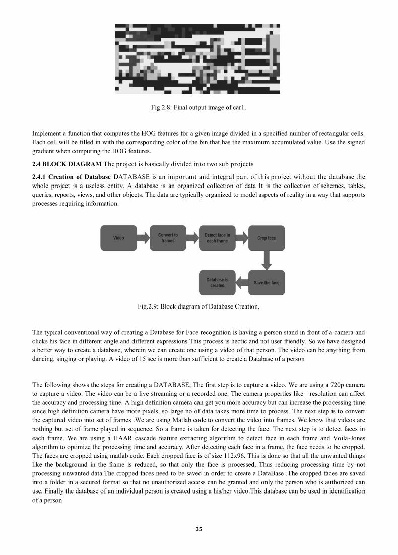
35

Fig 2.8: Final output image of car1.

Implement a function that computes the HOG features for a given image divided in a specified number of rectangular cells.

Each cell will be filled in with the corresponding color of the bin that has the maximum accumulated value. Use the signed

gradient when computing the HOG features.

2.4 BLOCK DIAGRAM The project is basically divided into two sub projects

2.4.1 Creation of Database DATABASE is an important and integral part of this project without the database the

whole project is a useless entity. A database is an organized collection of data It is the collection of schemes, tables,

queries, reports, views, and other objects. The data are typically organized to model aspects of reality in a way that supports

processes requiring information.

Fig.2.9: Block diagram of Database Creation.

The typical conventional way of creating a Database for Face recognition is having a person stand in front of a camera and

clicks his face in different angle and different expressions This process is hectic and not user friendly. So we have designed

a better way to create a database, wherein we can create one using a video of that person. The video can be anything from

dancing, singing or playing. A video of 15 sec is more than sufficient to create a Database of a person

The following shows the steps for creating a DATABASE, The first step is to capture a video. We are using a 720p camera

to capture a video. The video can be a live streaming or a recorded one. The camera properties like resolution can affect

the accuracy and processing time. A high definition camera can get you more accuracy but can increase the processing time

since high definition camera have more pixels, so large no of data takes more time to process. The next step is to convert

the captured video into set of frames .We are using Matlab code to convert the video into frames. We know that videos are

nothing but set of frame played in sequence. So a frame is taken for detecting the face. The next step is to detect faces in

each frame. We are using a HAAR cascade feature extracting algorithm to detect face in each frame and Voila-Jones

algorithm to optimize the processing time and accuracy. After detecting each face in a frame, the face needs to be cropped.

The faces are cropped using matlab code. Each cropped face is of size 112x96. This is done so that all the unwanted things

like the background in the frame is reduced, so that only the face is processed, Thus reducing processing time by not

processing unwanted data.The cropped faces need to be saved in order to create a DataBase .The cropped faces are saved

into a folder in a secured format so that no unauthorized access can be granted and only the person who is authorized can

use. Finally the database of an individual person is created using a his/her video.This database can be used in identification

of a person

36

2.4.2 Identification of a Person

Fig.2.10: Block diagram of Person Identification.

The following shows the steps in identification of a person

We have a camera to get live stream video .The camera properties like resolution can affect the accuracy and processing

time. A high definition camera can get you more accuracy but can increase the processing time since high definition camera

have more pixels, so large no of data takes more time to process. The video is converted to set of images to detect the faces.

We are using Matlab code to convert the video into set of images. We know that videos are nothing but set of frames played

in sequence. So a frame is taken for detecting the face. The next step is to detect faces in each frame .we are using a HAAR

cascade feature extracting algorithm to detect face in each frame and Voila-Jones algorithm to optimize the processing time

and accuracy. The next step is identifying the detected face. This is done by comparing the detected face with the Database.

We are using HOG feature extraction in order to compare the face and identify the detected face . The result is displayed

i.e. the details of the identified person is displayed.

2.5 RESULT ANALYSIS

Fig: 2.11: Example of Data Query Image

Fig: 2.12: Examples of Documents for Query Images

37

The purpose of face identification system is to identify criminals. In past years this process is carried out by

humans. This process gives the exact image of the criminal but it is very difficult to identify the criminal details and also it

requires much amount of human burden. The main aim of our project is to overcome the drawbacks of human based system

by using the machine based face identification process. In this process we store the details of criminal into the database

along with his photo or image. Then we make the image into different clips containing hair, forehead, eyes, nose, lips and

chin and store these clips into the database. When any crime occurs we compare the details given by the eyewitness with

the clips already stored in the database and we will identify the criminal. This project can be extended to adjust the gaps

between the clips after construction of the image to be a perfect photograph using Image processing Techniques.We were

able to create a new method to create a Database which is more user friendly than the conventional method. This can be

used in future more sophisticated creation of Database. Limitations of face recognition are Image quality affects how well

facial-recognition algorithms work, When a face-detection algorithm finds a face in an image or in a still from a video

capture, the relative size of that face compared with the enrolled image size affects how well the face will be recognized.

Even though high-definition video is quite low in resolution when compared with digital camera images, it still occupies

significant amounts of disk space.

In future, we would be able to see face recognition technology becoming the more advance security technology outdating

all other existing technologies

We are using this opportunity to express our gratitude to everyone who supported us throughout the course of this project.

We are thankful for their aspiring guidance, invaluably constructive criticism and friendly advice during the project work.

We are sincerely grateful to them for sharing their truthful and illuminating views on a number of issues related to the

project.

1. P. J. Phillips, J. Wechsler, J. Huang, P. Rauss, "The FERET database and evaluation procedure for face recognition

algorithms", Image and Vision Computing, vol. 16, no. 5, pp. 295-306, April 1998.

2. W. Zhao, R. Chellappa, P. J. Phillips, A. Rosenfeld, "Face recognition: A literature survey", ACM ComputSurv, vol.

35, pp. 399-458, December 2003.

3. M. Turk, A. Pentland, "Eigenfaces for recognition", J CognNeurosci, vol. 3, pp. 71-86, 1991.

4. P. N. Belhumeur, J. P. Hespanha, D. J. Kriegman, "Eigenfaces vs. Fisherfaces: Recognition using class specific

linear projection", IEEE Trans Pattern Anal Mach Intell, vol. 19, no. 7, pp. 711-720, July 1997.

5. H. A. Rowley, S. Baluja, T. Kanade, "Neural network-based face detection",Pattern Anal. Mach. Intell. IEEE Trans.,

vol. 20, no. 1, pp. 23-38, 1998.

6. M. V. Gupta, M. D. Sharma, "A Study of Various Face Detection Methods",METHODS, vol. 3, no. 5, 2014.

7. Kepenekci, B.; Akar, G.B, “Face classification with support vector machine,” Proc. IEEE Conf. Signal Processing

and Communications Applications, pp. 583-586, April 2004.

3. CONCLUSION

4. ACKNOWLEDGEMENTS

REFERENCES

38

ABSTRACT

DESIGN, ESTIMATION AND COSTING OF SEWAGE TREATMENT PLANT: A CASE STUDY

Adarsh S

Faculty of Civil Engineering Department

Vidya Vikas Institute of Engineering and Technology

Bannur Road, Alanahally

Mysuru-570028, Karnataka, India

9538438191

[email protected]

Shesha Prakash M N* Vice Principal, Professor and Head of Civil Engineering Department




9740011400,

[email protected]


Tejas S Pinaki, Darshan Paul Former Final year students, Department of Civil Engineering




Water scarcity has rightly occupied a prime concern due to migration of population from rural to urban areas. The

all important resource for sustenance of life is depleting at all levels, ie., above and below ground surface and needs to be

properly managed to make it more sustainable and available for future generations. The use of water, which has been

segregated based on its type of utilisation, has to be recycled and used for certain purposes. Over 70% of population across

the globe is unable to get access to drinking water. These aspects initiate the significance of design the economical

treatment plants.

Vidya Vikas Institute of Engineering and Technology (VVIET), is located at Alanahalli midway, (12018’13.3’’N

76042’36.9” E) between Mysore and Malavalli, having wide educational units starting from School to Master Degree which

educates around 4000 students every year. The campus is about 65 acres where half of the campus is filled with green

patches and lawn. There will be scarcity for water in campus during the early summer season itself due to less ground water

availability. Keeping this in mind, reuse of water is suggested by adopting Sewage Treatment Plant for the Girl’s hostel

which provides water for gardening and other recreational purposes.

A study on domestic wastewater characterization has been performed followed by the design of sewage treatment

plant. The present study involves the analysis of pH value, Total Dissolved Solids, Hardness, COD, BOD, DO, Nitrates,

Sulphates, Turbidity.



39

The study was conducted for the primary, secondary and tertiary treatment and management of sewage generated in VVIET

Girl’s hostel, a sewage treatment plant was designed. The total sewage generated in one day was estimated to be 25 KLD,

The various components of primary sewage treatment plant viz., screening chamber, Equalization and grit cum skimming

tank, settling tank, modified activated sludge tank, flash mixer and clari-flocculator, rough composite filter, disinfection

unit, sludge digester and sludge drying bed were designed considering the various standards and permissible limits of

treated sewage water.

It was recommended that the treated water will be supplied for flushing of WC, curing and gardening purpose and the

remaining sludge after treatment will be used as manure. The use of treated water will overcome the scarcity of ground

water within the campus and additionally the treated sludge will be very useful for increasing the fertility of soil.

Key Words: Vidya Vikas Institute of Engineering and Technology (VVIET), Sewage Treatment Plant (STP),

BOD, TDS, RCC Design, Estimation and Costing.

We are silently but surely heading towards “water shock” which will dwarf any oil crisis, because in the last two

decades for the first time in the human history more water is being taken out across the globe than what Nature is putting in.

Wastewater is used water, comprising of substances such as human waste, food scraps, oils, soaps, chemicals, domestic

wastes. Businesses and industries also contribute their share of used water/wastewater in addition to storm runoff burdened

with harmful substances via run off from roads, parking lots and rooftops and this can harm our fresh water systems. Even

though, nature has an amazing ability to cope with certain amounts of contaminants, there is a necessity to treat the billion

gallons of wastewater and sewage generated daily by homes, industries, and business establishments before releasing it

back to the environment (Ravi Kumar P et.al, 2010).

Degradation of water quality is the unfavourable alteration in chemical, physical and biological characteristics of water that

prevents domestic, commercial, industry, agricultural, and other beneficial uses of water. Sewage treatment plant is facility

designed to receive the waste from domestic, industrial and commercial sources and to remove materials that damage water

quality and compromise public health. Sewage is mainly composed of human fecal material, domestic wastes including

wash-water and industrial wastes (S Ramya et.al, 2015).

Currently, the interest in wastewater reuse in various parts of the world has promoted the development of wastewater and

secondary effluent treatment technologies. The main purpose of wastewater treatment is to prevent pollution of the

receiving watercourse, and to protect human health and the environment. The reuse of reclaimed wastewater is an

international practice. Due to the more and more pronounced water deficit, the reuse of wastewater in the Middle East

countries is part of the strategy for the conservation and development of water resources. Therefore, the investigation of the

characteristics of the reclaimed wastewater is necessary for evaluating its suitability for reuse (Al-Zboon, Kamel et.al,

2008). Wastewater or sewage treatment is one such alternative, wherein many processes are designed and operated in order

to mimic the natural treatment processes to reduce pollutant load to a level that nature can handle. In this regard, a detailed

characterization of the incoming wastewater based on the characterization a sewage treatment units were designed for

efficient treatment of sewage generated from the girl’s hostel and to prepare a detailed quantity estimate and costing for the

same was carried out.

Unit Operations of Sewage Treatment Plant The treatment plant should be located as near to the point of disposal as

possible. Care should be taken while locating the site that it should be on the downstream side and sufficiently away from

water intake works (Pramod Sambhaji Patil et.al, 2016).

Primary treatment systems are usually physical processes. Primary treatment alone will not produce an effluent with an

acceptable residual organic material concentration. Almost invariably biological methods are used in the treatment systems

to effect secondary treatment for removal of organic material. In biological treatment systems, the organic material is

metabolized by bacteria. Depending upon the requirement for the final effluent quality, tertiary treatment methods and/or

pathogen removal may also be included. Today majority of wastewater treatment plants use aerobic metabolism for the

removal of organic matter. The popularly used aerobic processes are the activated sludge process, oxidation ditch, trickling

1. INTRODUCTION

40

filter, and aerated lagoons. Stabilization ponds use both the aerobic and anaerobic mechanisms (Kavita N Choksi et.al,

2015). The different treatment methods used in wastewater treatment plant are classified in three different categories as:

Primary Treatment: Refers to physical unit operations.

Secondary Treatment: Refers to chemical and biological unit processes.

Tertiary Treatment: Refers to any one or combination of two or all three i.e., physical unit operations and chemical or

biological unit processes, used after secondary treatment.

Fig 2.1: Aerial view of Vidya vikas Institute of Engineering and Technology.

Vidya vikas Institute of Engineering and Technology (VVIET) is located in alanahalli midway, (12018’13.3’’N 76042’36.9”

E) between Mysore and Malavalli, and is spread over a sprawling campus of 65 acres with academic and administrative

buildings that are surrounded by a lush green ambience. VVIET is known for disciplined academic climate. Since its

inception, Vidya Vikas Educational Trust has catapulted into one of the leading educational institutions ranging from

primary schools to undergraduate and post graduate colleges covering the Arts, Commerce, Hospitality, Nursing, Social

Work, Law, and all facets of Engineering in the districts of Mysuru. Fig 2.1 depicts the Aerial view of study area.

3.1 Present Scenario: The UGD line of VVIET gir l’s hostel which accommodates near ly 220 students in 50 rooms

together connected to common manhole through a series of chambers. Fig 3.1 shows the proposed site for STP which is

located adjacent to VVIET Girl’s hostel block with an area of 60m x 60m. Block leveling for proposed STP was done using

total station. The site of area 50m x 50m is divided into blocks at an interval of 10m and the reduced level(RL) is recorded

along the longitudinal and cross section of the site. Fig 3.2 depicts the Contours plotted for the proposed STP site.

Fig 3.1: Proposed site for STP, located adjacent to VVIET Girl’s hostel with an area of 60m x 60m.

2. DESCRIPTION OF STUDY AREA

3. METHODS AND METHODOLOGY

41

Fig 3.2: Contour of the proposed site

3.2 Land Survey Block leveling for proposed STP was done using total station. The site of area 50m x 50m is divided

into blocks at an interval of 10m and the reduced level(RL) is recorded along the longitudinal and cross section of the site.

Fig 3.2 depicts the Contours plotted for the proposed STP site.

3.3 Collection of sample The sewage sample was collected through a Grab sampling technique, from the manhole

located at the corner of Hostel where the sewage from all the blocks flows into the manhole in a UGD. The sample is

collected three times (Morning, Afternoon and Evening) at the peak hours, for four consecutive days and then it is analyzed

in laboratory for various wastewater parameters. Fig 3.3 and 3.4 depicts the sample location and sample bottle after

collecting the sample from manhole.

Fig 3.3: Sampling location (Manhole) Fig 3.4: Sample collected in bottle

3.4 Laboratory Analysis Laboratory analysis was conducted for various wastewater parameters listed below as per

the standard procedures.

a. pH

b. BOD (Biochemical Oxygen Demand)

c. COD (Chemical Oxygen Demand)

d. TDS (Total Dissolved Solids)

e. Nitrates

42

f. Sulphates

g. Turbidity

4.1 Calculation of Quantity of sewage It is very difficult to ascertain the quantity of water required for a particular town.

It involves the assumptions of many variable factors and foresight of the designer plays an important role in arriving at this

quantity (K. Sesha Maheswaramma et.al, 2015). However the problem of estimating the quantity of water may be tackled

by studying in detailed the following two factors, they are rate of demand and population.

No of students: 220 No’s

Per capita demand: 135 LPCD

Percent Waste: 80%

Quantity of rain water: 1000 LPD

Influent BOD: 300mg/L

Operating cycle: 2 times per day

Total quantity of sewage: (220x135x0.8) + 1000=24760 ≈ 25000LPD OR 25KLD.

4.2 Operational units Based the wastewater characteristics, treatment units were designed. Those operations used

for the treatment of wastewater in which changes brought about by means of or through the application of physical forces

are known as unit operations. Fig 4.1 shows the flow diagram of sewage treatment plant.

Fig 4.1: Flow Diagram of Sewage Treatment Plant

M.H. = Manhole

1. Bar Screen

1.1 Equalization and grit and skimming unit

2. Modified activated sludge process

3. Settling chamber

4. Flash mixer and clarriflocculator

5. Rough composite filter

6. Disinfection unit

7. Polishing carbon filter

8. Sludge digester

9. Treated water tank

10. Sludge drying bed

M1

1.1 4 2

9

GIRLS

HOSTEL 2 2

10 6 5 8 7

3

4. DESIGN AND DETAILS OF SEWAGE TREATMENT PLANT UNIT

43

4.2.1 Bar screens The first unit operation encountered in wastewater treatment plant is screening. A screen is a

device with openings, generally of uniform size, that is used to retain the coarse solids found in wastewater. The screening

element may consist of parallel bars, rods or wings, grating, wire mesh, or perforated plate and the openings may be of any

shape but generally are circular or rectangular slots. Screens have openings (spaces between the bars) of 15mm at an angle

of angle of 45⁰ in the direction of flow. Bar screen should be either of epoxy-coated mild steel or stainless steel. Care is to

be taken to see that there are no gaps left between the screen frame and the floor and the sides of the chamber. Provide 60

cm wide and 80 cm deep drain section with bar screens of 2mmx4mm at 15 mm C-C at angle 450 in the direction of

flow. Bar screen should be either of epoxy coated mild steel or stainless steel. Care is to be taken to see that there are no

gaps left between the screen frame and the floor and the sides of the chambers the nuisance of odour coming from the

putrefying matter.

4.2.2 Equalization tank with grit cum skimming unit A grit chamber is generally not an essential unit in a typical

residential complex. It is however mandatory unit in commercial and industrial units with a canteen on campus.

A skimming tank is a chamber so arranged that floating matter rises and remains on the surface of the wastewater until

removed, while the liquid flows out continuously through deep outlets or under partitions, curtain walls or deep scum

boards. This may be accomplished in a separate tank or combined with primary sedimentation, depending on the process

and nature of the wastewater.

The equalization tank is the first collection tank in an STP. Its main function is to act as buffer: To collect the incoming raw

sewage that comes at widely fluctuating rates, and pass it on to the rest of the STP at a steady (average) flow rate.

During the peak hour sewage comes at the high rates. The equalization tank stores the sewage and lets it out during the non-

peak time when there is no/little incoming sewage. The operating cycles of the equalization tank is 2times per day.

V= 3

Assuming the depth of basin as 2.5 m

L x B = = 5 m2

Taking L = 3 m, L = length

L x B = 5 m2 B = breadth

B = =1.67m

Provide a equalization basin of (3 x 1.67 x 2.5) m.

0.5m = free board

0.8m = sludge depth

4.2.3 Modified ASP The aeration tank (together with the settling tank/clarifier that follows) is at the heart of the

treatment system. The bulk of the treatment system is provided here, employing microbes/bacteria for the process. The

main function of the aeration tank is to maintain a high population level of microbes. This mixture is called MLSS (mixed

liquor suspended solids). The mixed liquor is passed on to the clarifier tank, where the microbes are made to settle at the

bottom. The settled microbes are recycled back to the aeration tank. Thus they are retained for a long period within the

system.

Volume of ASP = V =

V = = 18.75 m3 ≈ 20 m3

Q0 = Inflow of sewage = 25 m3

c = solids retention time = 25d

Y = bio kinetic constant =0.5/d

S0=inflow BOD =300 mg/l

Se= Outflow BOD = 30 mg/l

X = MLSS=2000 mg/l

Kd = Decay rate = (0.05/d)

Let SWD = 3.0 m

44

L × B = = 6.66m2

Let us assuming L = 4 m

B = = 1.67 ≈ B = 2m

Provide (4 × 2 × 3) m for activated sludge unit.

0.3m = free board

4.2.4. Settling chamber Settling chamber is used for grit removal, particulate-matter removal in the primary settling

basin, biological-floc removal in the activated-sludge settling basin, and chemical-floc removal when the chemical

coagulation process is used. It is also used for solids concentration in sludge thickeners. In most cases, the primary purpose

is to produce a clarified effluent, but it is also necessary to produce sludge with a solids concentration that can be easily

handled and treated. In the design of sedimentation basin, considerations must be given to production of both a clarifier

effluent and a concentrated sludge.

Oxidized organics from ASP are settled in settling chamber.

Surface area of ST = A s= = 4.16 m2

Q = = =12.5 m3/cycle

Assume Outflow Rate =3 m/d

Assuming square settling chamber of size 3×3m, providing a SWD of 3m with 0.3m free board

and 0.5 m sludge depth

In flow and out flow arrangements

Inflow of biologically stabilized sewage is made by a rectangular chamber of c/s dimensions of 0.3m x 0.4m

Out flow is affected by a overflow channel of c/s dimensions of 0.5 ×0 .6m

4.2.5. Flash mixer with Clariflocculator Flash mixer with Clariflocculator Clariflocculator is a combination of

flocculation and clarification in a single tank to achieve economy in construction. It has two concentric tanks where inner

tank serves as a flocculation basin and the outer tank serves as a clarifier.

A flash mixing unit of (0.7× 0.6 ×0.5) m provided at the inlet of clariflocculator for rapid mixing of coagulant with effluent.

A clariflocculator of size 5m×4m is provided with 2 numbers of baffle walls for settling of flocs and side depth is 2 m, 1m

sludge depth. An additional 1m depth for sludge is provided. Outlet arrangement consists of a overflow channel of

dimension (0.7×0.6×0.5) m.

4.2.6. Filters Filtration is one of the principal unit operation used in the treatment of potable water. It is a well-

established operation for achieving supplemental removals of suspended solids (including particulate BOD) from

wastewater effluent of biological and chemical treatment processes. The role of filtration in the removal of effluent

suspended solids becomes even more firmly established.

4.2.7. Activated carbon filter It is light weight equipment which is aesthetic in appearance and easy to install, doesn’t

require concrete foundation. This filter uses the adsorption action of activated carbon. Activated carbon is typically

manufactured from coconut shell or charcoal, the “activation” process creating a highly porous material with a very large

surface area. Organic pollutant molecules are physically adsorbed and held fast within the catacomb-like porous structure of

the activated carbon. Granular activated carbon is typically used for this purpose.

4.2.7.1. Composite filter A rough composite filter is provided for the removal of any residual colloids from

clariflocculator. It is made up of locally available economic materials such as charcoal, brickbats, and pebbles. It is

provided with size of (2×2×2) m with free board 0.5m.

Filter media:

45

1st layer = 40mm brickbats of 0.5m deep

2nd layer = charcoal of 1m depth

3rd layer = pebbles of 0.5m depth

4.2.8. Disinfection chamber The various methods used for the disinfection are ozone, ultraviolet (UV) and chlorine.

The most common method of disinfecting wastewater is by the addition of chlorine. In most STPs, the common form of

Chlorine used is Sodium Hypochlorite (Hypo) available commercially at 10-12 % strength, being safe, easy to handle and

having a reasonable shelf life. For disinfection of pathogens in treated effluents bleaching powder is added in chamber of

(3×3×3) m with a free board of 0.3m.

4.2.9. Polishing carbon filter

It helps to remove turbidity suspended particles chlorine, organic matter, odour and colour present in the effluent.

In carbon filters adsorption process is involved.

4.2.10. Sludge digester Biological treatment of wastewater per force produces excess biological solids due to the

growth and multiplication of bacteria and other microorganisms in the system. The excess biomass thus produced needs to

be bled out of the system, and disposed off efficiently. This is a five-step process: sludge removal, storage, conditioning,

dewatering and disposal. Sludge is removed from the system from the sludge recirculation pipeline (through a branch). The

sludge is in the form of thick slurry. It is taken into a sludge-holding tank, and kept under aeration (to prevent the living

organisms from putrefying) until dewatering operations can be carried out. Before dewatering, polymer or other chemicals

may be added for conditioning the sludge, to facilitate the process. Sludge is then dewatered in a filter press/ Sludge bag/

centrifuge. The sludge digester is provided with size of 2m ϕ, height of 3m and free board of .97m.

4.2.11. Sludge drying bed: In order to dry the sludge obtained from various unit operations we are providing sludge

drying bed in brick masonry(in 1:4 CM) of size (3.0 x 2.0 x 2.0) m.

4.3 RCC Design The designed structural and reinforcement details are listed in the table 4.1 and 4.2 respectively.

4.3.1 R.C.C design of Equalization tank

Step 1: Tank dimensions:

Length= 3m,

Width= 1.67m,

Height=2.5+0.5(free board) +0.8(sludge depth) =3.8m

Specific weight/density of waste water =10.2KN/m3

Using M-30 grade concrete and HYSD bars (Fe-415)

Step 2: Permissible stress for M-30concrete and Fe – 415 steel

σcbc = permissible stress of concrete in bending = 10 N/mm2

σct= permissible stress of concrete in direct compression = 1.5 N/mm2

σst= permissible stress of steel in tension = 150 N/mm2

Step 3: Design constants:

m = modular ratio = 9.33

= 0.3834

j = 1-k/3 = = 0.8721

46

Q = 0.5× j×k× σcbc = 0.5×0.8721×0.3834×10 = 1.67 kN/mm2

Step 4: L = 3m, h = a = 3.8m, b = 1.67m

B/a= =0.44≈0.5

Mx = -0.035 @ y = 0

My = -0.029 @ y = b/2

Horizontal moment = Myωa3= 0.029 x 10.2 x 3.83=16.23 kN-m

Vertical moment = Mxωa3= 0.035 x 10.2 x 3.83 = 19.58kN-m

Thickness of wall is selected based on following three criteria

1. Thickness of wall should not be less than 150 mm

2. Thickness = 30H + 50 = 30 x 3.8 + 50 = 164 mm

3. =108.27 mm

Here we are adapting maximum of above value i.e. 164mm

Assume cover =40mm

Therefore, overall depth =165 + 40 (cover) = 205mm ≈ 210 mm

Effective depth, deff = 210 – 40 = 170 mm

Step 5: To find out the pull,

T = = 32.36 kN

Step 6: Check for stability:

< 1; σcbt=2 N\mm2, σct=1.5N\mm2 for M30 concrete

Tension is combined with horizontal moment

Therefore here moment, M = 0.029 x 10.2 x 3.83 = 16.23 kN-m

= 7.35X106 mm3

σcbt = = 2.208

σct| = = 0.242

= 1.265 > 1

Hence unsafe

Therefore, we need to increase thickness

i.e. 270 mm thickness of wall and select 12mm dia bars

deff = 270-40-12/2 =224 mm

=0.74 > 1

Hence safe, therefore we are adopting 270mm thickness of wall

Step 7: Design of base slab,

Ast min =0.3% of gross area = 0.003 x 1000 x 150 = 450mm2

Assuming thickness of base slab =150 mm

Providing =225 mm2 as main steel and distribution steel

Select 10 mm dia bars

47

Spacing = = 350 mm

Provide 10 mm dia bars @ 300 mm c/c as both main and distribution steel as both top and bottom

reinforcement.

The further units are designed using IS 3370-1967 and IS 456 – 2000 and the procedure adopted for the

design process is same as the above.

Design constants and parameters adopted for the design of treatment units:

The Specific weight/density of waste water =10.2kN/m3

Using M-30 grade concrete and HYSD bars (Fe-415)

Permissible stress for M-30concrete and Fe – 415 steel

σcbc = permissible stress of concrete in bending = 10 N/mm2

σct= permissible stress of concrete in direct compression = 1.5 N/mm2

σst= permissible stress of steel in tension = 150 N/mm2

Design constants:

m = modular ratio = 9.33

=0.3834

J = 1-k/3 = = .8721

Q = 0.5× j×k× σcbc = 0.5×.8721×.3834×10 = 1.67 kN/mm2

Note:

1. The slab thickness for the entire unit is 150mm. 2. The slab Reinforcements for entire unit is 10mm diameter at 300mm centre to centre

3. Sludge digester wall reinforcement horizontal wall is 400mm centre to centre and vertical walls is 12mm diameter at 200mm centre to centre

4. All dimensions are in mm

4.3Abstract of Estimated Cost The total abstract of estimated cost for the sewage treatment plant is given below in

the following table 4.2.

Table 4.1 : Structural Dimensions of the Sewage treatment units

Sl. No

Treatment unit

Dimensions (m)

length

width

depth Thickness (mm)

free

board depth

sludge

depth slab wall

1 Equalization and Grit cum

Skimming Tank 3 1.67 0.8 2.5 0.8 150 270

2 Modified ASP 4 2 0.3 2 150 230

3 Settling Chamber 3 3 0.3 3 0.5 150 270

4 Flash Mixer Clariflocculator 5 4 1 2.5 1 150 270

5 Rough Composite Filter 2 2 0.5 2 150 200

6 Disinfection Unit 3 3 0.3 3 150 200

7 Polishing Carbon Filter 2φ 0.54 3 150

8 Sludge digester 2φ 0.97 3 150 170

9 Treated water tank 6 6 3 150 300

10 Sludge drying bed 3 2 2 150 230

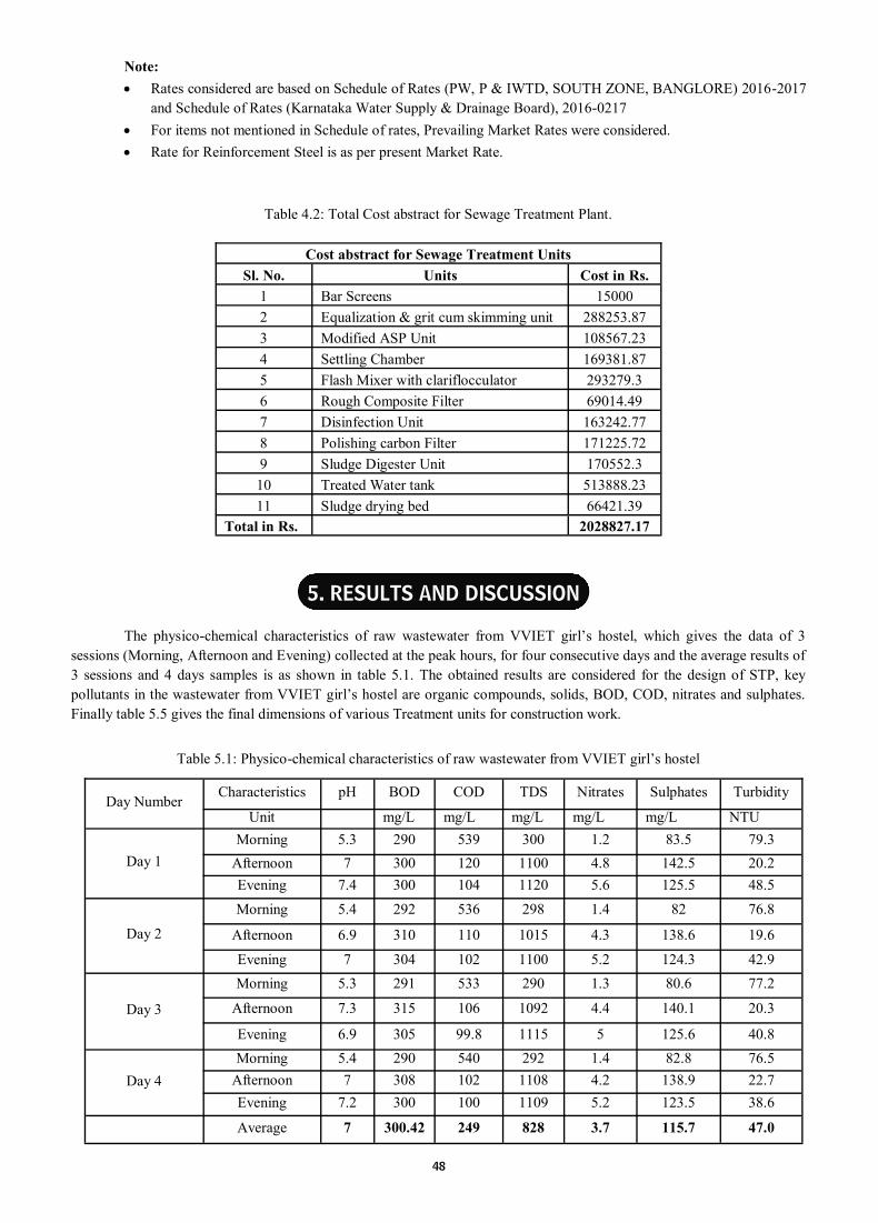
48

Note:

Rates considered are based on Schedule of Rates (PW, P & IWTD, SOUTH ZONE, BANGLORE) 2016-2017

and Schedule of Rates (Karnataka Water Supply & Drainage Board), 2016-0217

For items not mentioned in Schedule of rates, Prevailing Market Rates were considered.

Rate for Reinforcement Steel is as per present Market Rate.

Table 4.2: Total Cost abstract for Sewage Treatment Plant.

The physico-chemical characteristics of raw wastewater from VVIET girl’s hostel, which gives the data of 3

sessions (Morning, Afternoon and Evening) collected at the peak hours, for four consecutive days and the average results of

3 sessions and 4 days samples is as shown in table 5.1. The obtained results are considered for the design of STP, key

pollutants in the wastewater from VVIET girl’s hostel are organic compounds, solids, BOD, COD, nitrates and sulphates.

Finally table 5.5 gives the final dimensions of various Treatment units for construction work.

Table 5.1: Physico-chemical characteristics of raw wastewater from VVIET girl’s hostel

Cost abstract for Sewage Treatment Units

Sl. No. Units Cost in Rs.

1 Bar Screens 15000

2 Equalization & grit cum skimming unit 288253.87

3 Modified ASP Unit 108567.23

4 Settling Chamber 169381.87

5 Flash Mixer with clariflocculator 293279.3

6 Rough Composite Filter 69014.49

7 Disinfection Unit 163242.77

8 Polishing carbon Filter 171225.72

9 Sludge Digester Unit 170552.3

10 Treated Water tank 513888.23

11 Sludge drying bed 66421.39

Total in Rs. 2028827.17

Day Number Characteristics pH BOD COD TDS Nitrates Sulphates Turbidity

Unit mg/L mg/L mg/L mg/L mg/L NTU

Day 1

Morning 5.3 290 539 300 1.2 83.5 79.3

Afternoon 7 300 120 1100 4.8 142.5 20.2

Evening 7.4 300 104 1120 5.6 125.5 48.5

Day 2

Morning 5.4 292 536 298 1.4 82 76.8

Afternoon 6.9 310 110 1015 4.3 138.6 19.6

Evening 7 304 102 1100 5.2 124.3 42.9

Day 3

Morning 5.3 291 533 290 1.3 80.6 77.2

Afternoon 7.3 315 106 1092 4.4 140.1 20.3

Evening 6.9 305 99.8 1115 5 125.6 40.8

Day 4

Morning 5.4 290 540 292 1.4 82.8 76.5

Afternoon 7 308 102 1108 4.2 138.9 22.7

Evening 7.2 300 100 1109 5.2 123.5 38.6

Average 7 300.42 249 828 3.7 115.7 47.0


49

Table 5.2: Final Dimensions of various Treatment units for construction work.

The present paper works as a template for the similar designs of Sewage Treatment Plants (STP) which can be

ready reckoner. Further this will be a motivation for implementing such treatment plants in line with our Prime Minister’s

National slogan, Swach Bharath. In addition, the cost of the entire STP has been optimized to reduce it to a meager

percentage of the total cost of the associate building. A detailed Design, Estimation and Costing of Sewage Treatment Plant

for VVIET Girl’s Hostel were done. Available site area is found to be 60m x 60m and utilized area for the construction of

STP is 50m x 50m. Care was taken while selecting a site such that it is on the downstream side so that wastewater can flow

through the gravity where pumping cost will be reduced. Total quantity of wastewater to be treated is 25 KLD. Based on

the results obtained, adoption of two filters in the treatment process ensures the better treatment of sewage and hence

treated sewage could be used for gardening, flushing in Water closet and even treated water can be utilised for drinking

purpose as higher degree of treatment is given to the wastewater generated. The sludge obtained from the sludge

drying beds can be used for the gardening purpose within the campus. Surplus sludge can be sold out for reasonable price as

it can be used as manure in agricultural fields. The overall estimated cost of the project is Rs. 20, 28,827 (Twenty lakh

twenty eight thousand eight twenty two seven rupees).

1. Al-Zboon, Kamel and Al-Ananzeh, Nada (2008) “Performance of wastewater treatment plants in Jordan and suitability

for reuse” African Journal of Biotechnology 7 (15), pp. 2621-2629.

2. B G Mahendra and Prema (2013) “Performance Evaluation of Existing Waste Water Treatment Plant” International

Journal of Research in Engineering and Technology IJRET pp.294-297.

3. Kavita N. Choksi, Margi A. Sheth, Darshan Mehta (2015) “To evaluate the performance of Sewage Treatment Plant: A

Case study” International Research Journal of Engineering and Technology IRJET 4(8) pp.1076-1080.

4. K. Sesha Maheswaramma, N.Babavali, K.Satyanarayana, K. Etheshamul Haq, K.Renuka (2015) “Design of Water

Treatment Plant to Pulivendula Municipal Corporation of Kadapa (Dt), Andhra Pradesh”. International Journal of

Research in Engineering and Technology IJRET 4(2) pp.2319-2321.

5. Pramod Sambhaji Patil, Shaikh Hujefa, Nemane Rahu Mujawar Sumer, Deo Prasad, Chaudhari (2016) “Design of

Sewage Treatment Plant for Dhule City” International Journal of Engineering Research IJER 5(5) pp.353-355.

6. Ravi Kumar P, Liza Britta Pinto, Somashekar R K (2010) “Assessment of the Efficiency of Sewage Treatment Plants:

A Comparative Study between Nagasandra and Mailasandra Sewage Treatment Plants” Kathmandu University Journal

of Science, Engineering and Technology 6(1) pp.115-125.

7. S. Ramya, Aswani Krishna P, Athulya babu O C, Harsha K Rajan (2015) “Design of Sewage Treatment Plant and

Characterisation of Sewage” National Conference on Research Advances in Communication, Computation, Electrical

Science and Structures NCRACCESS pp.2348-2353.

SLNo Treatment units Dimensions (in m)

1 Bar screens (in line with outfall drain) (0.60 wide×0.80 deep) cm

2 Equalization & grit cum skimming unit 3.0×1.670×(2.50+0.80)

3 Modified ASP unit 4.0x2.0x(2+0.3)

4 Settling chamber 3.0x3.0×(3+0.3+0.5)

5 Flash mixer and clariflocculator 5.0×4.0×(2.50+1)

6 Rough composite filter 2.0×2.0×(2.0+0.5)

7 Disinfection unit 3.0×3.0×(3.0+0.3)

8 Polishing carbon filter 2.0φ×(3.0+0.54)

9 Sludge digester unit 2.0φ×(3.0+0.97)

10 Treated water tank 6.0×6.0×3.0

11 Sludge drying bed 3.0×2.0×2.0

REFEENCES

6. CONCLUSIONS

50

ABSTRACT

ANALYSIS OF BOOST CONVERTER USING DIFFERENT PID TUNING TECHNIQUES

COMPARED WITH CLOSE LOOP SYSTEM

Kiran H. Raut Assist. Professor

Electrical Engineering Department,

G. H. Raisoni Academy of Engineering And Technology, Nagpur

phone no.9623246144

E-mail:- [email protected]

The use of DC –DC power converters is continuously growing both in power electronics products & system. DC-

DC converters are used to convert one DC voltage to another DC voltage. It is inordinately used in industry as well as in

research. The major drawback of the boost converter is the uncontrolled supply of voltage and current. So initially

convectional PID controller is designed to regulate the output voltage and shows improved performance of the converter

when compared to close loop system.

Keywords: PID Controller, Boost converter, Tuning Techniques, MATLAB Simulation .

Power converter has played very important role for handling high power. DC-DC converters are some of the

simplest power electronic converter circuits. They are widely used in the power supply equipment for most electronic

instruments and also in specialized high power applications such as battery charging, plating and welding. The wide variety

of circuit topologies ranges from the single transistor buck, boost and buck/boost converters to complex configurations

comprising two or four devices and employing some techniques to control the switching losses. The usual requirement of a

control system for the converter is to maintain the output voltage constant irrespective of variations in the DC source

voltage Vin and the load current. However, load changes affect the output voltage transiently, possibly causing significant

deviations from the steady state level. Furthermore, in a practical system circuit losses introduce an output voltage

dependency on steady state load current which must be compensated for by the control system [1,2 ,3].

PID controller is being used in 90% of industries[6]. PID is extensively used for it is simple in structure and has standard

performance for most of the industries. But it is quite challenging to find gains of PID to meet response time and overshoot

(phase margin) specifications. Manual tuning is purely trial and error process, time consuming and non-systematic. It may

not produce optimal design and can lead to dangerous conditions. So some standard design procedures had been introduced

like Ziegler-Nichols method, Chien-Hrones-Reswick method and pure numerical optimization approach . For analysis of a

control system first a mathematical model of the boost converter is derived by state space averaging techniques [7]. The

transfer function Thus obtained is used to find the gains of controllers by different tuning methods mentioned above.

In this paper in section II basic theory of PID controller is given. In Section III gives basic idea of DC to DC boost

converter.In section IV & V design of boost converter with control transfer function is presented [8]. In section VII different

1. INTRODUCTION


51

tuning methods are discussed and their respective compensator transfer functions are given. Various tuning methods are

compared in section XI with system characteristics. Finally the tuning method with best performance is chosen and is

implemented to designed boost converter.

Proportional-Integral-Derivative (PID) controller has been used for several decades in industries for process

control applications. PID involves three separate parameter, the proportional, the integral and derivatives. By tuning the

three constants in PID controller algorithm, the controller can provide control action designed for specific process

requirement.

Fig.1 Block representation of PID Controller in a close loop system

This method is more popular among all control methods. The determination of proportional (KP), derivative (Kd) and

integral (Ki) constants are known as tuning of PID controller. A PID controller is shown in Figure 1 and is given by

Where Kc = proportional gain, Ti = integral time constant and Td = derivative time constant. The introduction of

integral action facilitates the achievement of equality between the measured value and the desired value, as a constant error

produces an increasing controller output. The introduction of derivative action means that changes in the desired value may

be anticipated, and thus an appropriate correction may be added prior to the actual change. Thus, in simplified terms, the

PID controller allows contributions from present, past and future controller inputs.

In case of DC to Dc boost converter, average output voltage is always higher than the input voltage.

Fig.2 DC-DC Boost Converter

(2)

2. MODEL OF PID CONTROLLER

3. DC – DC BOOST CONVERTER

52

Inductor is used to resist the change in current supplied. The boost converter is operating as follow.

1. When switch S is close, Inductor stores the energy into it. Current is circulating in clockwise direction. Left side

polarity of inductor is positive. When switch S is open, current is decrease. And inductor opposes the change of current

into it. For that polarity will be reverse. i.e. Left side of inductor is negative in this situation.

2. Switch “S” is in ON state, current through inductor is increase. And diode is in off condition. Switch “S” is in OFF

state, the current stored in inductor is now coming out through diode [4]. On the basic of Faraday’s low we can

conclude that,

Vin DT = (Vin-V0) (1-D)T

Vin = Input DC voltage,

Vo = Output DC voltage,

D = Duty cycle,

T = Total time

In the switch ON, state inductor is been charged as source voltage of Vg and capacitor will discharge. The equation of

duty cycle (D) is become [5].

As per voltage balance equation, we can see that

Vg (DTs) + (Vs – Vo) (1-D) Ts = 0

Vg(DTs) –Vg(DTs) – VgTs + Vo DTs – VoTs = 0

Boost converters are switched power converters. The converter uses a transistor switch, typically a MOSFET, to

pulse width modulate the voltage into an inductor.

Duty Cycle (D): To determine the duty cycle D, for the minimum input voltage. The minimum input voltage is used

because it leads to the maximum switching current.

D= 1-( / )

Vin = Input voltage

Vo = Desired output voltage

Load Resistance (R): R= /

Vo = desired output voltage

Io = desired output current

Inductance (L): L= ⁰( − )/Δ ⁰ ⁰

Δ =10%

Vin = input voltage

Vo = desired output voltage

fs = switching frequency

Δ = inductor ripple current


Capacitance (C): C=( ⁰ ) /( ⁰Δ )

4. DESIGN CALCULATION OF BOOST CONVERTER

53

Δ = ( 1− +Δ 2)


D = duty cycle

fs = switching frequency

Δ = output ripple voltage

Δ = inductor ripple current

ESR = equivalent series resistance of the capacitor

Table 1. Design Specification

The modeling of DC-DC boost converter is carried out to determine the state space model. The output and the

control transfer function of the system are obtained from the state space model using MATLAB. This method is known as

state space averaging technique. The operation of the boost converter takes place in two modes.

Switch ON equivalent circuit

Fig 3: Boost converter- ON mode

During ON mode as shown in Fig 2, the state equation matrices are given by-

Sr. No. Parameters Values 1 Input Voltage (Vin) 60 V 2 Input Current (Iin) 5 A 3 Output Voltage (Vo) 300 V 4 Output Current (Io) 1 A 5 Duty Cycle (D) 0.8

6 Load Resistance (R) 300 Ω 7 Inductance (L) 240 mH 8 Equivalent Series Resistance (ESL) 0.5 Ω 9 Capacitance (C) 5000 μF

10 Equivalent Series Resistance (ESR) 16 mΩ

5. STATE SPACE MODELING

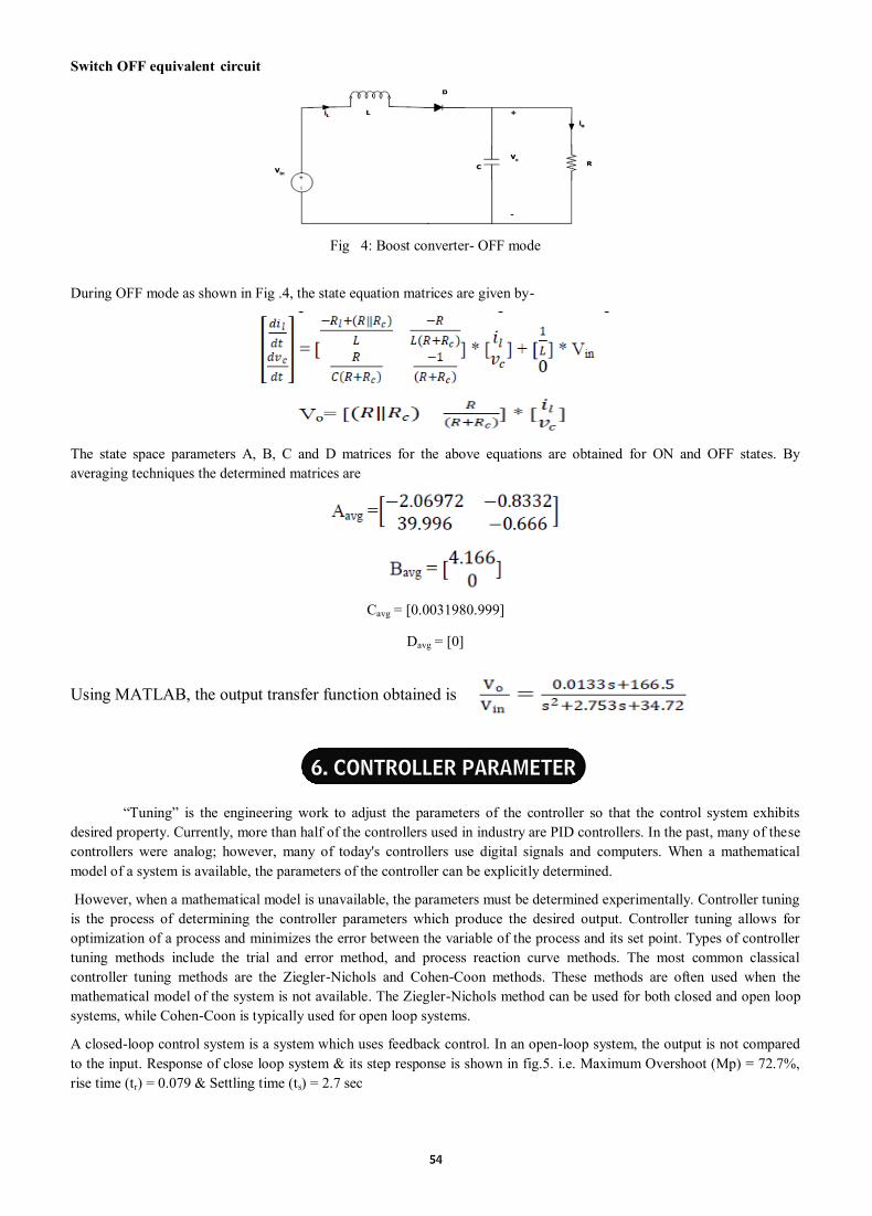
54

Switch OFF equivalent circuit

Fig 4: Boost converter- OFF mode

During OFF mode as shown in Fig .4, the state equation matrices are given by-

The state space parameters A, B, C and D matrices for the above equations are obtained for ON and OFF states. By

averaging techniques the determined matrices are

Cavg = [0.0031980.999]

Davg = [0]

Using MATLAB, the output transfer function obtained is

“Tuning” is the engineering work to adjust the parameters of the controller so that the control system exhibits

desired property. Currently, more than half of the controllers used in industry are PID controllers. In the past, many of these

controllers were analog; however, many of today's controllers use digital signals and computers. When a mathematical

model of a system is available, the parameters of the controller can be explicitly determined.

However, when a mathematical model is unavailable, the parameters must be determined experimentally. Controller tuning

is the process of determining the controller parameters which produce the desired output. Controller tuning allows for

optimization of a process and minimizes the error between the variable of the process and its set point. Types of controller

tuning methods include the trial and error method, and process reaction curve methods. The most common classical

controller tuning methods are the Ziegler-Nichols and Cohen-Coon methods. These methods are often used when the

mathematical model of the system is not available. The Ziegler-Nichols method can be used for both closed and open loop

systems, while Cohen-Coon is typically used for open loop systems.

A closed-loop control system is a system which uses feedback control. In an open-loop system, the output is not compared

to the input. Response of close loop system & its step response is shown in fig.5. i.e. Maximum Overshoot (Mp) = 72.7%,

rise time (tr) = 0.079 & Settling time (ts) = 2.7 sec

6. CONTROLLER PARAMETER

55

Fig.5 Close loop response of the system

The Z-N tuning rule was discovered by Ziegler and Nichols in the year 1942[9].

This procedure is only valid for open loop stable plants and it is carried out through the following steps

i. Set the true plant under proportional control, with a very small gain.

ii. Increase the gain until the loop starts oscillating. Note that

linear oscillation is required and that it should be detected at the controller output.

iii. Record the controller critical gain K p = Kcr and the oscillation period of the controller output, Pcr.

iv. Adjust the controller parameters according to Table 2.

After applying above procedure, the step response for the Kp = Kcr=200 .

Table 2: Ziegler –Nichols Tuning setting

Therefore, Kcr = 200 ,Pcr= 0.35 second .Obtain PID parameters from Table 2. KP = 120 ,Ki = 0.291 & Kd = 0.0437 step

response is shown in fig.6. Mp = 46%, tr = 0.00368 & ts = 0.0418 sec.

Fig.6. Time response of Ziegler-Nichols method

7. ZIEGLER-NICHOLS (Z-N) METHOD

PID Type Kp Ti Td

PID 0.6Kcr Pcr/2 Pcr/8

56

For some control loops the measure of oscillation, provide by ¼ decay ratio and the corresponding large

overshoots for set point changes are undesirable therefore more conservative methods are often preferable such as modified

Z-N settings These modified settings that are shown in Table.3. Are some overshoot (10).

Table 3: Modified Ziegler –Nichols Tuning setting

As per Table 3, for some overshoot KP = 66, Ki =1/Ti = 0.175 and Kd = 0.116, with the above values of KP, Ki and Kd, step

response is shown in Fig.7. Mp = 42.8%, tr =0.00324 & ts = 0.0363 sec.

Fig.7. Response for Modified Ziegler –Nichols Tuning Method

The Tyreus-Luyben procedure is quite similar to the Ziegler–Nichols method but the final controller settings are

different [11]. This method is applicable for PI and PID Controller .This method are based on ultimate gain period and

period given in table .4.

Table 4 : Tyreus – Luyben Parameter

As per Table 4, KP = 62.5, Ki =1/Ti = 0.777 and Kd = 0.055, with the above values of KP, Ki and Kd, step response is shown

in Fig.8. Mp = 43.9%, tr = 0.00368 & ts = 0.0517 sec.

8. MODIFIED ZIEGLER-NICHOLS TUNING METHOD

Type of controller

Parameter

Kp Ti Td

Some Overshoot 0.33 Kcr Pcr/2 Pcr/3

9. TYREUS-LUYBEN METHOD

Type of con-

troller

Parameter

Kp Ti Td

PID Controller 0.59 Kcr Pcr /6 Pcr /1.5

57

Fig.8. Response for Tyreus- Luyben Method

In many cases, plants are not allowed to undergo through sustained oscillations, as is the case for tuning using

continuous cycling method. Damped oscillation method is preferred for these cases. Damped oscillation method is invented

by Harriott. The optimum settings for a P-I-D controller are shown in Table [12]

Table 5 : Harriott Tuning Parameters

As per Table 5, KP = 118, Ki =1/Ti = 0.0583 and Kd = 0.233, with the above values of KP, Ki and Kd, step response is shown

in fig.9. Mp = 37%, tr = 0.00162 & ts = 0.0153 sec.

Fig.9.Response for Damped Oscillation Method

Different PID tuning methods are discussed in this paper. Step response of all methods and their system

characteristics are compared with close loop system. Total four PID tuning techniques were implemented and their

performances analyzed. The system exhibits a largest peak overshoot and settling time with Ziegler Nichols tuning

technique. Damped oscillation method exhibits smallest maximum overshoot and settling time. Among the four PID tuning

techniques, the damped oscillation tuned PID controller gives the best results for a second order system.

10. DAMPED OSCILLATION METHOD

Type of con-

troller

Parameter

Kp Ti Td

PID Control-

ler Kcr /3.2 Pcr /0.45 Pcr /6.3

11. CONCLUSION

58

Table 6: Time response parameters

1. Hebertt J. Sira-Ramirez & Ramón Silva-Ortigoza, Control Design Techniques in Power Electronics Devices,

Springer-Verlog, 2010

2. Mohan, Undeland and Robbins. Power Electronics: Converters, Applications and Design. – Wiley, 1989.

3. B.K.Bose, Power Electronics and Variable Frequency Drives,IEEE press, 1997.

4. X.Felix Joseph, Dr.S.Pushpakumar, D.Arun Dominic, D.M.Mary Synthia Regis Prabha, “Design and Simulation of a

soft switching scheme for a dc-dc Boost Converter with pi controller”, International Journal of Engineering (IJE),

Volume: (4).

5. Tarak Salmi, Mounir Bouzguenda, Adel Gastli, Ahmed Masmoudi “MATLAB/Simulink Based Modelling of Solar

Photovoltaic Cell” International Journal of Renewable Energy Research, Vol.2, No.2, 2012.

6. C. Lee. A Survey of PID Controller Design based on Gain and Phase Margins. International Journal of

Computational Cognition, 2004, 2(3): 63–100.

7. Robert Priewasser, Member, IEEE, Matteo Agostinelli, Member, IEEE, Christoph Unterrieder, Member, IEEE,

Stefano Marsili, Member, IEEE, and Mario Huemer, Senior Member, IEEE; “Modeling, Control and Implementation

of DC-DC Converter for Variable Frequency Operation”, IEEE Transactions on Power Electronics, Vol. 29, No.1,

January 2014.

8. [2] Hyun-Hee Park and Gyu-Hyeong Cho, Senior Member, IEEE; “A DC-DC Converter for a Fully Integrated PID

Compensator with a Single Capacitor”, IEEE Transactions on Circuits and Systems-II: Express Briefs, Vol. 61, No.

8, August 2014.

9. Ziegler, J.G. and N.B. Nichols, ―Optimum Settings for Automatic Controllers‖, Trans. ASME, Vol. 64, pp.759-768

(1942).

10. Kiran H.Raut and Dr.S.R.Vaishnav “International Journal of Innovative Research in Electrical, Electronics,

Instrumentation and Control Engineering”, “Performance Analysis of PID Tuning Techniques based on Time

Response Specification”, Volume 2, issue 1, jan 2014.

11. Finn Haugen,” Comparing PI Tuning Methods in a Real Benchmark Temperature Control System”, Modeling,

Identification and Control, Vol. 31, No. 3, 2010, pp. 79-91.

12. K. Ogata: “Modern Control Engineering”, Prentice-Hall India, Fourth Edition.

Algorithm Rise Time

(Tr)

Maximum Over-

shoot (Mp)

Settling time

(Ts)

Z-N Method 0.0036 46 0.0418

Modified Z-N Method 0.0032 42.8 0.0363

Tyreus – Luyben 0.0047 43.9 0.0517

Damped Oscillation Method 0.0016 37 0.0153

REFERENCES

59

ABSTRACT

DESIGN AND DEVELOPMENT OF CONSTANT PRESSURE DELIVERING PUMP

Amit L. Meshram

PG Scholar, Department of Mechanical Engineering,

Priyadarshini College of Engineering, RTM Nagpur University

Nagpur, Maharashtra, India.

[email protected]

Sagar D. Shelare* Assistant Professor, Department of Mechanical Engineering,



Tel No. +91-9890027265

[email protected]

*Corresponding Author

Machchhendra K. Sonpimple Professor, Department of Mechanical Engineering,



[email protected]

Water pressure is one of the major problems today we are facing in domestic, agriculture and industrial sector

since in all cases the initial requirement is to provide the water at high pressure. To maintain proper boosting pressure in

commercial buildings and all other purposes, hydro pneumatic pump can be used. These pumps are highly energy efficient

if we maintain a set pressure level whereas if we use constant speed booster systems it will tends to waste of energy. Hydro

pneumatic system are generally installed in the basement of a building for the convenience of the user on the other end of a

fixture side, at any given time. Boosters have a simple job; they “charge” the system with pressurized water such that as

soon as tap is opened on an upper floor, the water is available immediately for the user. This reality has its inherent

“inefficiencies” since many times throughout the day, the pump must either re-start to replenish any lost water in the system

or continue to run as the water is disbursed to the fixture throughout the day. Sometimes these “occasional” loads can last

throughout the day, this phenomenon realize that this run-time was costing more money. Hence the work of construction,

designing and selecting of various accessories is being carried out in industry which is given in this paper.

Keywords: Control Panel; discharge; losses; manifold; pressure.

A pump is a machine which is used to raise the pressure of the liquid and to move the liquid with pressure from

one place to another. A pump can be further defined as a machine that uses several energy which gets transform to increase

the pressure of a liquid. The transfer of liquids against gravity existed from time immemorial. A pump is one such device

1. INTRODUCTION

60

which is used energy to raise, transport, or compress liquids. Pumps are widely used in industrial and residential

applications. Pumping equipment is extremely diverse, varying in type, dimensions, size, and materials of construction

used. There have been significant new developments are in the area of pumping equipment, early 1980s. Every year vast

tonnage of liquid in the form of solid-liquid or semisolid mixtures, known as slurries. The application which involves the

largest quantities is the dredging industry, continually maintaining navigation in harbors and rivers, altering coastlines and

winning material to used to landfill and construction purposes. Dredging is one of the most common type and one of the

ancient process involving slurry flows; the dredged materials contain a wide range of particles, tree debris, rocks, etc.

Mining is one of the concept employed slurry flows in pipelines since the mid-nineteenth century, when the technique was

used to reclaim gold from placers in California. Long-distance slurry pipelines have evolved in all continents since the mid-

1950s. Some slurry mixtures consist of very fine solids at high concentration; other mixtures are based on coarse particles

up to a size of 150 mm. Pumps are normally classified as: Reciprocating, Rotary, Centrifugal etc. in this project we utilize

centrifugal pump.

Centrifugal pump works on the basic principle of forced vortex flow, which means that when a certain mass of liquid is

rotated by an external flow, there will be rise in pressure head of the rotating liquid takes place by pump. The rise in

pressure head at any point of the rotating/ moving liquid is proportional to the square of tangential velocity of the liquid at

that point. Hence at the outlet side of the impeller where the radius is more, the rise in pressure head will be more and the

liquid will be discharged at the outlet with high pressure. Due to high-pressure head, the liquid can be lifted to a high level.

Figure shows flow of fluid in a centrifugal pump. When the pump is in operation there will be an increase in the fluid

pressure from the pump inlet to its outlet. This pressure difference drives the fluid through the system or plant. The

centrifugal pump increase in pressure by transferring mechanical energy of motor to the fluid through the rotating impeller.

The fluid flows from the inlet to the impeller center and out along its blades. The centrifugal force increases the fluid

velocity and consequently also the kinetic energy is transformed to pressure.

Fig1. Principle of centrifugal pump

A. Pump: The CR pump is a vertical inline multistage pump. This pump type is also able to pump corrosive fluids because

the hydraulic parts are made of stainless steel or titanium.

B. Pressure Transducer: Pressure switches are used for maintaining the predetermined pressure differentials in the

pressure tank. They are used as pilot circuits for starting the pump when the pressure in the tank reaches the low

operating limit and again to stop the pump when the high operating limit is reached.

C. Pressure Relief Valve: Pressure relief valves are used to protect the system against damage because of either excessive

water or air pressures. They are the safety valves of the system and, therefore, should be checked frequently to keep

them in the best operating condition. They should be set to operate at a safe value above the maximum system pressure

but always within the safe working limits of the tank or other parts which are to be protected and also selected with

sufficient capacity to vent off all excess pressure.

D. Pressure Gauge: Pressure gauges are used for indicating the pressures existing in the system.

2. MAIN COMPONENTS

61

E. Strainers: Strainers are placed on the end of the water drain valves to protect the system against entrance of any

possible contamination.

F. Air Filters: Air filters are placed on the intake lines to the air compressor, air inlet valves and vent connections when

and as required. They are used to protect the system from atmospheric contaminations.

G. Check Valves: Thoughtful specification and selection of check valves for use in the piping lines of pneumatic pressure

systems contributes to installation efficiency. Noisy, slamming valves should not be tolerated and definitely have no

place in systems supplying hospitals, sanitariums, hotels and similar installations where noise is detrimental and a

nuisance.

H. Base Plate: Base plate is the firm steel structure which is used to stand the complete assembly. It is provided to

absorb shock, provide damping and provide the base.

I. Suction Manifold: Suction manifold is the essential need of any pump, in this project as the pump is of negative type

hence specially design suction manifold is used in project.

J. Delivery Manifold: Delivery manifold are used to deliver pump water to the required section.

K. Hydro pneumatic Tank: Hydro pneumatic tank basic purpose is to maintain proper pressure and flow control. Two

factors should be considered when specifying the construction of the pressure tank. They are the minimum safe

working pressure which the tank must withstand in service and the possibility of corrosion which will affect the

anticipated safe working life of the tank.

L. Control Panel: Control panel is being provided to the system in which various system are provided such as VFD, PLC

and IO etc.

In modelling process CREO 2.0 have been used to developed different parts of the model which are necessary.

I. Inlet Skid:

Straight pipe: 5D-10D = 5x100 – 10x100 Length L = 720mm.

Flange= 100 mm, 8 holes dia 18, pcd 180mm. Eccentric reducer with flange= 100mm -150mm.

Ball valve = 150mm Straight pipe 2 = 200mm.

Long bend elbow 60º = 150mm Straight pipe 3 =1500mm

Fig. 2. Inlet Skid

3. COMPUTER AIDED MODELLING

62

II. Outlet Skid:

Outlet of the pump vary as per the requirement for this project we have taken the standard diameter 100mm

Fig. 3. Outlet Skid

I. Selection of Pump:

Head = 40 m, V=0.707m/s, Diameter= 0.1m

Q = A x V (1)

Applying Darcy formula we get,

Hf = 4*0.01*1500*0.707² / 2*9.81*0.1 = 15.28 m

NPSH = atmospheric pressure – elevation correction – vapor pressure –suction head

= 33.96 - 1.2 - 6.675 – 3 = 29.08 feet = 8.86m

NPSH required = 1.56 m, NPSH available = 8.86 m

On the above basis standard vertical centrifugal pump has been selected and its specification are as follows:

Table 1. Technical Specification

4. DESIGN OF HYDRAUPNUEMATIC

PRODUCT NAME CR 24-2-1 PRODUCT NAME CR 24-2-1

Technical Materials

Speed for pump data 2919 rpm Pump housing Cast iron

Rated flow 20.5 m³/h Pump housing EN-JL1030

Rated head 46.6 m Pump housing ASTM A48-30B

Head max 58.8 m Impeller Stainless steel

Impellers 4 Impeller DIN W.-Nr. 1.4301

Primary shaft seal HQQE Impeller AISI 304

Approvals on nameplate CE,TR Material code A

Curve tolerance ISO9906:2012 3B Code for rubber E

Pump type CR 20 Bush material Graflon

Stages 4

Pump version A

Model A

63

II. Design of Pipe:

Inside diameter of pipe: d = 1.13 √(Q/v) = 1.13√(0.33/42.42) = 0.099m = 100mm (2)

III. Wall thickness of pipe:

According to thin cylinder formula, wall thickness is: T = pd/2σt (3)

For design of pipe certain constant is added,

T = pd/2σt + c = 5x100/2x14 + 3 = 25mm (4)

Where c = 3 for MS, σ= 14 N/mm² for MS

Pressure drop in pipe: ∆p = [Q/cA]² x d/2 = 0.0153 bar (5)

IV. Stresses in Pipe:

According to LAMIS equation,

Tangential stress (σt) = [p(ri²)/(ro² - ri²)] x [1+ (ro²/x²)] = [5(100²)/ (125² - 100²)]

x [1+ (125²/100²)] = 10.25 MPa (6)

Where, p = internal fluid pressure, Ri = internal radius of pipe, Ro = outer radius of pipe.

Radial stress (σr) = [p (ri²) / (ro² - ri²)] x [1- (ro²/x²)] =

[5(100²)/ (125² - 100²)] x [1- (125²/100²)] = -2.25 Mpa (7)

V. Design of Flanged Joint:

D= 100mm, p=5bar, c=3, σt= 14

Thickness of pipe:T = pd/2σt + c = 5x100/2x14 +3 = 25mm (8)

Where c = 3 for MS, σ= 14 N/mm² for MS

Other dimensions of flange:

PRODUCT NAME CR 24-2-1 PRODUCT NAME CR 24-2-1

Installation Electrical data

Maximum ambient temper-

ature 60 °C Motor type 132SC

Max pressure at stated temp 16 bar / 120 °C IE Efficiency class IE3

Max pressure at stated temp 16 bar / -20 °C Rated power - P2 5.5 kW

Flange standard DIN Power (P2) required by

pump 5.5 kW

Connect code F Mains frequency 50 Hz

Pipe connection DN 50 Rated voltage 3 x 220-240 D/380-415 Y

Pressure stage PN 16 Rated current 36,0-34,5/20,8-19,8

Flange size for motor FF265 Starting current 660-780 %

Liquid Cos phi - power factor 0.88-0.84

Pumped liquid Water Rated speed 2920-2940 rpm

Liquid temperature range -20 to 120 °C Efficiency IE3 91.2%

Liquid temp 20 °C Motor efficiency at full

load 91.2-91.2 %

Density 998.2 kg/m³ Motor efficiency at 3/4

load 91.80%

Motor efficiency at 1/2

load 91.30%

Number of poles 2

Enclosure class (IEC 34-5 55 Dust/Jetting

Insulation class (IEC 85) F

Motor protect PTC

Motor No 85U07417

64

Nominal diameter of bolt: d= 0.75t + 10mm = 28mm (9)

Number of bolts: N = 0.0275d + 1.6 = 4 (10)

Thickness of flange: Tf = 1.5t + 3 = 40.5mm (11)

Width of flange: B= 2.3d = 64.4 = 66mm (12)

Outside diameter of flange: Do = d + 2t + 2B = 28 + 2x25 + 2x66 = 282mm (13)

Pitch circle diameter of bolt: Dp = D + 2t + 2d = 100 + 2x25 + 2x28 = 206mm (14)

Circumferential pitch of bolt: Pc = ᴨ x Dp / n = ᴨ x 206 / 4 = 161.71mm (15)

In order to make the joint leak proof, the radius of Pc should be in between 20√d1 to 30√d1 value.

D1 = diameter of bolt hole = d + 3 = 31mm

20√d1 = 113.35; 30√d1 = 167.03

Since circumferential pitch is in between 20√d1 to 30√d1, hence design is safe.

VI. Selection of Butterfly Valve:

As pipe diameter = 100mm, hence standard butterfly valve is selected, its technical specification are:

Valve body = cast iron ASTM A126 class GG25, Valve disc = stainless steel AISI 316, epoxy coating.

Valve seat = EPDM standard, Shaft bushing = PTFE lubricated plated steel.

Top flange = ISO 5211 standard, Pressure rating: 200 PSI/16 bar for ANSI125/150 flange

Temperature rating:

Working temp min +46ºf (+8ºc) Max +230ºf (+110ºc), Design temp min -4ºf (-20ºc) Max +248ºf (+120ºc)

VII. Assembly of Pump:

Fig. 4. Assembly of Pump

An experimentation is being carried out in Industry considering the various working aspects such as discharge

obtained per unit time, pressure obtained per unit time and power consumed per unit discharge. Readings obtained after

experimentations are:

5. EXPERIMENTAL ANALYSIS

65

Table 2. Experimental Data

Graphs are very useful to correlate the behaviour of various aspects. Therefore graphs are plotted between discharge

obtained per unit time, pressure obtained per unit time and power consumed per unit discharge.

Fig. 5 . Time Vs Discharge

From Fig. 5, it has been seen that as the discharge or requirement is zero, in such case pump will directly shut off itself.

Fig. 6 . Pressure Vs Time

From Fig. 6, it has been seen that when we set the pressure of the pump at 3 bar and we started the pump initially it will

start at lower pressure level and then gain the required pressure, suddenly at 70 sec when we close the valve, pressure

suddenly increase in such case system will get shut off.

Discharge Vs Time Pressure Vs Time Power Vs Discharge

Discharge

(m³/hr.)

Time

(hrs.)

Time

(sec)

Pressure

(bar)

Discharge

(m³/hr.)

Power

(kw)

10 1 10 1.5 0 0

5 2 20 1.9 5 2

0 3 30 2.4 10 2.7

30 4 40 2.9 15 3.2

25 5 50 3.1 20 3.7

40 6 60 3 25 3.97

45 7 70 3.4 22 3.75

30 8 80 3.2 12 2.8

66

Fig. 7.Power Vs Discharge

Fig. 7 shows the power requirements as per the discharge condition at 25 m³/hr power require is 3.97kw, as discharge level

goes down at 12 m³/hr power required is 2.8kw.

Table 3. Actual Performance

Fig. 8. Actual Performance Curve 1

Head Q (m³/hr.) ETA (%) Pump

40 5 40 1

40 10 58 1

40 15 68 1

40 20 72 1

40 25 67.5 1

40 29 67.5 1

40 30 67.5+64 1 + 2

40 35 67.5+70 1 + 2

40 40 67.5+74 1 + 2

40 45 67.5+70 1 + 2

40 50 67.5+67.5 1 + 2

67

Fig. 9. Actual Performance Curve 2

From Fig. 8, it is observed that as pump is running at constant head 40m, if we maintain a discharge of 25 m³/hr. then pump

1 will start working from 0 m³/hr. to 25 m³/hr., at the same time we observe that ETA performance is increasing after

achieving a constant height it start decreasing so as to maintain the efficient system as show in graph 1. As when the

discharge level goes beyond the 25 m³/hr. than 2nd pump comes into operation to maintain the pressure and discharge in the

system. VFD allows both pump to run but in an efficient manner as shown in Fig. 9.

Comparison of Hydro Pneumatic pump with Conventional Pump has been carried out considering the various variables

such as Power, Efficiency and Cost. The results are as shown in Fig. 10 and Fig. 11:

Fig 10: Efficiency Comparison

Fig 11: Cost Comparison

6. COMPARISON OF HYDRO PNEUMATIC PUMP AND

CONVENTIONAL PUMP

68

Conclusions obtained by above results are

At no discharge or when requirement is zero, in such case pump will directly shut off itself. When the requirement is

zero at discharge point pump get automatically switch off.

When we set the pressure of the pump at 3 bar and we started the pump initially it will start at lower pressure level and

then gain the required pressure, suddenly after some time when we close the valve, pressure suddenly increase in such

case system will get shut off.

Power requirement is directly proportional to requirement of discharge condition. Through with the help of VFD power

is saved.

Pump 1 runs upto predetermined discharge. As discharge level goes above the limit of pump 1 then automatically 2

pump starts running to maintain the constant pressure.

Pump setup is installed in the premises of Textile Industry Nagpur, after successful implementation and trial problem

of pressure and discharge has been eliminated.

Hydro pneumatic pump is much more efficient as compared with conventional pump with respect to head, discharge,

efficiency, power and cost etc.

1. Ludwig, D. Meschkat, S. and Stoffel, B.. Design Factors Affecting Pump Efficiency. Presented at the 3rd

International Conference on Energy Efficiency in Motor Driven Systems, Treviso, Italy, September 18-20, 2002,

p.532-538.

2. Stepanoff, A.J. Centrifugal and axial flow pumps: theory, design and application, John Wiley & Sons, 2nd

edition,1957.

3. Fox, R. and McDonald A. (1998) Introduction to Fluid Mechanics, John Wiley & Sons, 5th edition,1998.

4. Cernetic, J. The use of noise and vibration signals for detecting cavitation in kinetic pumps. Proc. IMechE Vol. 223

Part C: Jnl. Mech. Eng. Science, 2009, p. 1645-1655.

5. Hydraulic Institute . ANSI/HI 1.3-2000 – Rotodynamic (Centrifugal) Pumps for Design. 2000.

6. Hydraulic Institute . ANSI/HI 9.8-1998 – American National Standard for Pump Intake Design. 1998

7. American Society of Mechanical Engineers ASME . ASME/ANSI B16.1-2005 – Gray Iron Pipe Flanges and

Flanged Fittings: Classes 25, 125, and 250. 2005.

8. American Society of Mechanical Engineers . ASME/ANSI B31.1-2007 – Power Piping. American Society of

Mechanical Engineers. 2007.

9. Casada, D.. Energy and reliability considerations for adjustable speed driven pumps, Presented at Industrial Energy

Technology Conference, Houston, USA 1999, p. 53-62.

10. Meshram, A.; Sonpimple, M.K. and Shelare, S.D. A Case Study on Pump of Hydropneumatic Booster System.

Presented at the 4th International conference on Recent Innovation in Science Engineering Management, India

International Centre, New Delhi, March 20, 2016, p. 167.

7. CONCLUSIONS

REFERENCES

69

ABSTRACT

DESIGN AND DEVELOPMENT OF DROP WEIGHT GENERATOR FOR HARNESSING GREEN ENERGY

Mahesh K Professor EEE

New Horizon College of Engineering,

Bangalore-560103

Mobile: 09900119252

[email protected]

Lithesh J* New Horizon College of Engineering,

Bangalore-560103

Mobile: 9164609997

[email protected]

* Corresponding author

Sujith A New Horizon College of Engineering,

Bangalore-560103

Mobile: 7829372534

[email protected]

Conserving energy has become the biggest issue in present scenario. Due to the development and modernization

the electricity demand is increasing at high extent. To fulfil this demand globally which is without any harmful effect on

environment is possible by using gravity power generation which is part of green energy. The reason behind generating

power by using gravity is that it is available all over the earth. Comparing to the other sources like chemical, thermal and

other sources gravity is weak, is scalable. This weakness is due to uniformity, or steady state of our interactions with

gravity. The concept of Drop Weight Generator is simple. The basic concept of gravity power generation mechanism is,

when a body moves down from higher altitude to lower one its potential energy is converted into kinetic energy. This

motion is converted into circular motion and that circular motion is converted into electricity by using a single phase

synchronous generator.

Keywords: Conservation of Energy, Green Energy, Drop weight, Gravity, potential energy, kinetic energy, single phase

synchronous generator.

Now a days due to the effects of pollution and global warming there is a need for generating power from renewable

sources. Due to the availability of gravity all over the earth, abundant and consistent it is very suitable to generating power

by using gravity. Energy demand is increasing day by day with rapid growth in industrialization as well as modernization.

1. INTRODUCTION




70

But the energy resources are gradually decreasing at high extent. Within a few years the energy resources will be finished

and hence there will be lack of fuel (coal, wood, water, etc.) for power generation. The other renewable sources such as

solar, wind, biomass etc are available only for a particular duration of time during the day and night. Therefore the Drop

weight generator is one of the method to generate power which fulfils energy demands and requirements of present time [1]

[12][13].

It is possible to deflect gravitational action away from an object so that the object is partially deviated. That effect makes it

possible to extract energy from the gravitational field, which makes the generation of Drop weight generator

technologically feasible.

Gravitational force is force that attracts any object with mass (weight)[4]. The

primary objective is to provide a gravity power generation mechanism which

can continuously convert gravity potential energy into kinetic energy. This

motion is converted into circular motion and is then converted into electricity

using an Alternator .Fig 1 shows project model.

Drop weight generator has advantages over the hydro-electric plant, such as

not needing of fuel and not polluting the environment. However, the Drop

weight generator would be much smaller than hydro-electric plants. The

location of that plant would not be restricted to suitable water elevations and

Drop weight generator and their produced energy would be much expensive. If

the gravitational power electric generation comes under operation and working

then it can replace all existing nuclear and fossil fuel plants and it would

essentially solve the problem of global warming to the extent it is caused by

fossil fuel used.

Fig 1: Project model

Fig 2:Block Diagram

Components of the block diagram are as shown in Fig 2:

Alternator

Wheel arrangement

Rope and drum arrangement

Weight (Driving force)

Load

2. BLOCK DIAGRAM OF DROP WEIGHT GENERATOR

71

Alternator An alternator is an electrical generator that converts mechanical energy to electrical energy in the form

of alternating current. For reasons of cost and simplicity, most alternators use a rotating magnetic field with a

stationary armature. Occasionally, a linear alternator or a rotating armature with a stationary magnetic field is used. In

principle, any AC electrical generator can be called an alternator, but usually the term refers to small rotating machines

driven by automotive and other internal combustion engines. An alternator that uses a permanent magnet for its magnetic

field is called a magneto. Alternators in power stations driven by steam turbines are called turbo-alternators. Large 50 or

60 Hz three phase alternators in power plants generate most of the world's electric power, which is distributed by electric

power grids[6].

By Excitation There are two main ways to produce the magnetic field used in the alternators, by using permanent

magnets which create their own persistent magnetic field or by using field coils. The alternators that use permanent magnets

are specifically called magnetos. In other alternators, wound field coils form an electromagnet to produce the rotating

magnetic field.

All devices that use permanent magnets and produce alternating current are called PMA or permanent magnet alternator. A

"permanent magnet generator" (PMG) may produce either alternating current, or direct current if it has a commutator. If the

permanent magnet device makes only AC current, it is correctly called a PMA.

The fig 3 shows a design of revolving field generator and the generator is to have the armature part on stator and

the magnetic field part on rotor. A basic design of revolving field single-phase generator is shown on the right. There are

two magnetic poles, north and south, attached to a rotor and two coils which are connected in series and equally spaced on

stator. The windings of the two coils are in reverse direction to have the current to flow in the same direction because the

two coils always interact with opposing polarities. Since poles and coils are equally spaced and the locations of the poles

match to the locations of the coils, the magnetic lines of force are cut at the same amount at any degree of the rotor. As a

result, the voltages induced to all windings have the same value at any given time. The voltages from both coils are "in

phase" to each other. Therefore the total output voltage is two times the voltage induced in each winding. In the figure, at

the position where pole number 1 and coil number 1 meet, the generator produces the highest output voltage on one

direction. As the rotor turns 180 degrees, the output voltage is alternated to produce the highest voltage on the other

direction. The frequency of the AC output in this case equals to the number of rotations of the rotor per second.

Fig 3:Revolving field design

This design can also allow us to increase the output frequency by adding more poles. In this example on the right, we have

4 coils connected in series on the stator and the field rotor has 4 poles. Both coils and poles are equally spaced. Each pole

has opposite polarity to its neighbours which are angled at 90 degrees. Each coils also have opposite winding to its

neighbours. This configuration allows the lines of force at 4 poles to be cut by 4 coils at the same amount at a given time.

At each 90-degree rotation, the voltage output polarity is switched from one direction to the other. Therefore, there are 4

cycles of the AC output in one rotation. As the 4 coils are wired in series and their outputs are "in phase", the AC output of

this single-phase generator will have 4 times the voltage of that generated by each individual coil.

A benefit of the revolving field design is that if the poles are permanent magnets, then there is no need to use any slip ring

and brush to deliver electricity out of the generator as the coils are stationary and can be wired directly from the generator

to the external loads [7][8]

3. REVOLVING FIELD DESIGN

https://en.wikipedia.org/wiki/Generator_(device)

https://en.wikipedia.org/wiki/Alternating_current

https://en.wikipedia.org/wiki/Armature_(electrical_engineering)

https://en.wikipedia.org/wiki/Linear_alternator


https://en.wikipedia.org/wiki/Electrical_generator


https://en.wikipedia.org/wiki/Electrical_generator

https://en.wikipedia.org/wiki/Magnetic_field

https://en.wikipedia.org/wiki/Magneto

https://en.wikipedia.org/wiki/Magnetic_field

https://en.wikipedia.org/wiki/Magneto

https://en.wikipedia.org/wiki/Three_phase

https://en.wikipedia.org/wiki/Electric_power_grid

https://en.wikipedia.org/wiki/Permanent_magnet

https://en.wikipedia.org/wiki/Magneto_(generator)

https://en.wikipedia.org/wiki/In_phase

https://en.wikipedia.org/wiki/In_phase

72

A conductor moving relative to a magnetic field develops an electromotive force (EMF) in it (Faraday's Law). This emf

reverses its polarity when it moves under magnetic poles of opposite polarity. Typically, a rotating magnet, called

the rotor turns within a stationary set of conductors wound in coils on an iron core, called the stator. The field cuts across

the conductors, generating an induced EMF (electromotive force), as the mechanical input causes the rotor to turn. [3]

The rotating magnetic field induces an AC voltage in the stator windings. Since the currents in the stator windings vary in

step with the position of the rotor, an alternator is a synchronous generator.

The rotor's magnetic field may be produced by permanent magnets, or by a field coil electromagnet. Automotive alternators

use a rotor winding which allows control of the alternator's generated voltage by varying the current in the rotor field

winding. Permanent magnet machines avoid the loss due to magnetizing current in the rotor, but are restricted in size, due

to the cost of the magnet material. Since the permanent magnet field is constant, the terminal voltage varies directly with

the speed of the generator. Brushless AC generators are usually larger than those used in automotive applications.

An automatic voltage control device controls the field current to keep output voltage constant. If the output voltage from the

stationary armature coils drops due to an increase in demand, more current is fed into the rotating field coils through

the voltage regulator (VR). This increases the magnetic field around the field coils which induces a greater voltage in the

armature coils. Thus, the output voltage is brought back up to its original value. [2]

Alternators used in central power stations also control the field current to regulate reactive power and to help stabilize the

power system against the effects of momentary faults. Often there are three sets of stator windings, physically offset so that

the rotating magnetic field produces a three phase current, displaced by one-third of a period with respect to each other

[9].The Arrangement is shown in Fig 4 and Fig 5.

Fig 4: Wheel arrangement

Fig 5: Rope, drum and load arrangement

Load

The load can be a lamp or a battery that is to be charged or any other low voltage devices. The generated output can be used

for charging laptops and mobile phones. In this case, we require rectifiers in order to convert the generated AC voltage to

DC voltage. Car alternators usually have inbuilt rectifiers and hence this output can be used directly to charge mobile

phones and laptops.

4. PRINCIPLE OF OPERATION

https://en.wikipedia.org/wiki/Rotor_(electric)

https://en.wikipedia.org/wiki/Rotating_magnetic_field


https://en.wikipedia.org/wiki/Voltage_regulator

https://en.wikipedia.org/wiki/Power_station

https://en.wikipedia.org/wiki/Fault_(power_engineering)

https://en.wikipedia.org/wiki/Three_phase

73

The driving force here is the Weight and gravitational force. The Weight drives the wheel and the alternator shaft. The

diameter of the wheel is 26 inches whereas that of the alternator shaft is 1 inch. This makes the gear ratio to be 26:1. This

implies one rotation of the wheel would make the alternator shaft rotate 26 times. The Fig 6 shows the gear ratio.

Fig 6: 26:1 gear ratio

The alternator being

used is a Car Alternator. This alternator has three terminals as shown in Fig 7 and namely

Field supply terminal

Output terminal ( Armature )

Ground terminal (Body).

Fig 7: Alternator terminals

Field Excitation

Automotive alternators require a voltage regulator which operates by modulating the small field current to produce a

constant voltage at the battery terminals. Early designs (c.1960s-1970s) used a discrete device mounted elsewhere in the

vehicle. Intermediate designs (c.1970s-1990s) incorporated the voltage regulator into the alternator housing. Modern

designs do away with the voltage regulator altogether; voltage regulation is now a function of the electronic control

unit (ECU). The field current is much smaller than the output current of the alternator; for example, a 70 A alternator may

need only 7 A of field current. The field current is supplied to the rotor windings by slip rings. The low current and

relatively smooth slip rings ensure greater reliability and longer life than that obtained by a DC generator with its

commutator and higher current being passed through its brushes. [2]

5. WORKING OF DROP WEIGHT GENERATOR

https://en.wikipedia.org/wiki/Voltage_regulator

https://en.wikipedia.org/wiki/Electronic_control_unit

74

Fig 8: Field of an alternator

The field windings are supplied with power from the battery via the ignition switch and regulator. A parallel circuit supplies

the "charge" warning indicator and is earthed via the regulator.(which is why the indicator is on when the ignition is on but

the engine is not running). Once the engine is running and the alternator is generating power, a diode feeds the field current

from the alternator main output equalizing the voltage across the warning indicator which goes off. The wire supplying the

field current is often referred to as the "exciter" wire. The drawback of this arrangement is that if the warning lamp burns

out or the "exciter" wire is disconnected, no current reaches the field windings and the alternator will not generate power.

Some warning indicator circuits are equipped with a resistor in parallel with the lamp that permit excitation current to flow

if the warning lamp burns out [5]. The driver should check that the warning indicator is on when the engine is stopped;

otherwise, there might not be any indication of a failure of the belt which may also drive the cooling water pump. Some

alternators will self-excite when the engine reaches a certain speed. The field of the alternator is shown in Fig 8

Efficiency of automotive alternators is limited by fan cooling loss, bearing loss, iron loss, copper loss, and the voltage drop

in the diode bridges. Efficiency reduces dramatically at high speeds mainly due to fan resistance. At medium speeds

efficiency of today's alternators is 70-80%. This betters very small high-performance permanent magnet alternators, such as

those used for bicycle lighting systems, which achieve an efficiency around 60%. Larger permanent magnet electric

machines (that can operate as motors or alternators) can achieve today much higher efficiencies. Pellegrino et al., for

instance, propose not particularly expensive designs that show ample regions in which efficiency is above 96%. Large AC

generators used in power stations run at carefully controlled speeds and have no constraints on size or weight. They have

very high efficiencies as high as 98%.

Advantages of Electro magnets over Permanent magnets

Permanent magnet strength depends upon the material used in its creation. The strength of an electromagnet can be

adjusted by the amount of electric current allowed to flow into it. As a result, the same electromagnet can be adjusted

for different strength levels.

If a permanent magnet loses its magnetic properties, as it does by heating to a (maximum) temperature, it will be

rendered useless and its magnetic properties can be only recovered by re-magnetizing. Contrarily, an electromagnet

loses its magnetic power every time an electric current is removed and becomes magnetic once again when the electric

field is introduced

A permanent magnet’s magnetic properties exist when the magnet is (magnetized). An electromagnetic magnet only

displays magnetic properties when an electric current is applied to it. That is how you can differentiate between the

two. The magnets that you have affixed to your refrigerator are permanent magnets, while electromagnets are the

principle behind AC motors.

The main advantage of an electromagnet over a permanent magnet is that the magnetic field can be quickly changed by

controlling the amount of electric current in the winding. [10][11].

6. ADVANTAGES

https://en.wikipedia.org/wiki/Bicycle_lighting_systems

https://en.wikipedia.org/wiki/Permanent_magnet

75

Advantages of Alternators over DC Generator (Dynamos)

The alternator will produce its rated output at a much lower RPM than will the generator. This is a great advantage.

The alternator is mechanically simpler than generator, it does not have the brushes that wear out, so the alternator

normally last much longer with no maintenance.

For producing same output the size of DC generator is much bigger than an alternator.

They are lighter, cheaper and more rugged.

They use slip rings providing greatly extended brush life over a commutator.

The brushes in an alternator carry only excitation current, a small fraction of the current carried by the brushes of a DC

generator, which carry the generator's entire output. A set of rectifiers (diode bridge) is required to convert AC to DC.

To provide direct current with low ripple, a three-phase winding is used and the pole-pieces of the rotor are shaped

(claw-pole) to produce a waveform similar to a square wave instead of a sinusoid. Automotive alternators are

usually belt driven at 2-3 times crankshaft speed. The alternator runs at various RPM (which varies the frequency)

since it is driven by the engine. This is not a problem because the alternating current is rectified to direct current.

Advantages of the Project

The power is readily available any time.

Can be implemented for various ratings.

Continues energy conversion is possible with small energy input

Eco friendly, pollution free Green energy.

This energy source will remain forever.

The Drop Weight Generator mechanism of the present invention utilizes a gravity energy conversion unit which

can provide a continuous and stable operation to convert the gravity potential energy into kinetic energy and finally into

electric energy to perform a long-time, effective and stable energy output. The present invention not can independently

generate electricity and can also be connected to wind power and solar power generation systems to generate electricity.

This paper envisages a power generation mechanism that produces power from gravity having a simplified structure. It is

eco-friendly and could overcome present problems of pollution and global warming faced by other power generation

methods.

1. Vidhan Srivastava, Sumit Chaudhary, Shailesh M. Pandey, KulvinderRana “ Gravity Power Generation” IJMRS’s

International Journal of Engineering Sciences, Vol. 01, Issue 03, September 2012.

2. George.O. Schur, “Gravity actuated thermal motor”, United States Patent number: 4121420.

3. Richard P Feynman, Robert B Leighton ,Matthew Sands “ Lecture on physics”, Narosa book disributirs ltd., volume

1.

4. Chun-chao Wang, Yuh-suiang Wang “Gravity Power Generation Mechanism” United States patent number:

20090115195 A1 App No.11/935,228 May, 2009.

5. Victor Rene AnguloValpreda, Mayra Palomares Coral US 8344537 B2 App No. 12/668,757 January,2013.

6. David Hatcher Childress Anti-gravity and the Unified field Adventures Unlimited press Pages: 6,38,106,204,545

May,1990.

7. CONCLUSION

REFERENCES

https://en.wikipedia.org/wiki/Slip_ring

https://en.wikipedia.org/wiki/Belt_(mechanical)

76

7. John. J. Hurford, “Gravity motor ”, United States Patent number: 6237342.

8. Md.Muqtar Ahmed, HeenaNaaz, "Power Generation through Gravity and Kinetic Energy", International Journal of

Scientific and Research Publications, Volume 4, Issue 1, January 2014.

9. Digvijay S, Sagar N, Nitin N, “Gravity Power Generation” International jouranal of advance research in science and

engineering. ISSN-2319-8354, Volume No. 5, Issue No.3 march 2016.

10. Rakesh s. Ambade, RoushanPrabhakar, Rupesh s. Tayade, “Review on Gravity Power Generation”, International

Innovative Research in Science, Vol. 3, Issue 4, April 2014. PP1, 2, 3.

11. Vidhan Srivastava, Sumit Chaudhary, Shailesh M. Pandey, KulvinderRana “Gravity Power Generation” JMRS’s

International Journal of Engineering Sciences, Vol. 01, Issue 03, September 2012.

12. H.C.Verma, “Concepts of Physics-1”, BharatiBhawan (Publishers & Distributors), 2008.

13. Md.Muqtar Ahmed, HeenaNaaz, "Power Generation through Gravity and Kinetic Energy", International Journal of

Scientific and Research Publications, Volume 4, Issue 1, January 2014.

77

ABSTRACT

EMPLOYEE ENGAGEMENT: EMPIRICAL EVIDENCE ON RECENT REPORTS

G. Swetha, * Associate Professor,

Department of Management Studies,

Sri Padmavathi college of Computer Sciences and Technology,

Mohan gardens, Vaishnavi Nagar, Thiruchanoor, Tirupati-517503

[email protected]


Pradeep Kumar Professor & Head,

Department of Management Studies,

Madanapalle Institute of Technology & Science, Madanapalle

[email protected]

Employee Engagement has been a buzz word in Human Resource Management. Managers are inducing companies to

implement engagement strategies in order to increase profits and reduce attrition rate. Engaging employees is one of the

top five most important challenges for management, according to a survey of 656 chief executive officers (CEOs) from

countries around the world (Wah 1999). Employee engagement has become the top issue on the minds of business leaders,

directing us to an entirely new model of management. The objective of this paper is to present a brief review on recent

reports of Employee Engagement. The authors through this paper offer a comprehensive review of latest reports that are

available to date.

Key words: Engagement, commitment, productivity, retention and loyalty.

Employee engagement has emerged as a critical driver of business success in today’s competitive marketplace. Further,

employee engagement can be a deciding factor in organizational success. Not only does engagement have the potential to

significantly affect employee retention, productivity and loyalty, it is also a key link to customer satisfaction, company

reputation and overall stakeholder value. Thus, to gain a competitive edge, organizations are turning to HR to set the agenda

for employee engagement and commitment. Thus, to foster a culture of engagement, HR leads the way to design measure

and evaluate proactive workplace policies and practices that help attract and retain talent with skills and competencies

necessary for growth and sustainability.

Employee Engagement is defined as “the extent to which employees commit to something or someone in their organization,

how hard they work and how long they stay as a result of that commitment.”[1]

1. INTRODUCTION



78

Employees who are engaged have a positive attitude about their organization and job. They are always enthusiastic to learn

about new things. They often exhibit loyalty towards the organization. Engaged employees always go extra mile for the

growth of individual and organizational development. They are hard working and always contribute to the overall success

of the company.

In fact, there are many pathways to encourage Engagement, however only one ‘kit’ does not fit to all the organizations.

While each organization may define Employee Engagement differently, ultimately, the key to effective Engagement will be

rooted in the flexibility of approach most appropriate for each individual firm.

We know from many research institutions and studies, that companies which focus on engaging their employees typically

enjoy better profits, a happier workforce and improved productivity. For example, here are just a handful of the statistics;

Highly engaged employees are 38% more likely to have above-average productivity.

Source: Workplace Research Foundation

Employees who report feeling valued by their employer are 60% more likely to report they are motivated to do their

very best for their employer.

Source: American Psychology Association / Harrison Interactive

Companies who implement regular employee feedback have turnover rates that are 14.9% lower than for employees

who receive no feedback.

Source: Gallup

Increasing employee engagement investments by 10% can increase profits by $2,400 per employee, per year.

Source: Workplace Research Foundation

There are number of advantages due to engaged employees in the organization.

Engaged employees strive for the company’s development and growth. Employees who are engaged in the

organization leads to positive results like increased sales & profits and enhancing organization’s reputation in the

corporate world.

Employees who are engaged take pride in their work which means they are careful at work and have lower rate of work

accidents and mistakes.

They enjoy going to work which reduces absenteeism in the organization.

Engaged employees also tend to stay longer in their jobs which have less turnover and reduces recruitment cost.

In this era, one of the biggest challenges for the organizations are not just retaining talented employees, but fully engaging

them for the growth and development of the company.

According to Deloitte Global Human Capital Trends (2014) research, 78% of business leaders opine that retention and

engagement are the important and urgent issues to focus for the growth of the organizations.

According to Blessingwhite report, research confirms that four out of 10 workers are disengaged globally. According to

State of the American workplace Report, 70 percent of U.S. employees don’t like their job, emotionally disconnected from

their workplace and disengaged.

Research (source: www.blessingwhite.com) shows four out of 10 workers are disengaged globally. In the U.S., the situation

is worse. According to the latest State of the American Workplace Report, 70 percent of U.S. workers don’t like their job,

creating an environment where many workers are emotionally disconnected from their workplace and less productive than

engaged counterparts.

2. WHY EMPLOYEE ENGAGEMENT

3. ADVANTAGES OF EMPLOYEE ENGAGEMENT

4. IT'S TIME TO RETHINK ABOUT 'EMPLOYEE ENGAGEMENT'

http://www.deloitte.com/hctrends

http://www.blessingwhite.com/EEE__report.asp

http://www.blessingwhite.com

http://www.gallup.com/strategicconsulting/163007/state-american-workplace.aspx

79

The change what organizations need today is instead of measuring Engagement annually, redefine engagement in the

organization. It must be a continuous and holistic approach. If employees really love their work and there is supportive

environment in the organization, then they treat customers in a better way, innovates new products in the market and

continuously strive for the improvement of the organization.

We can’t “retain” people; we can only “attract them.” We can’t “engage them” but we can “inspire and support them.” We

can’t only “train them” but we can “enable them to learn” and “give them the opportunities to develop.”

Let’s change our thinking and move beyond the concept of employee satisfaction that is engagement. If organizations really

want to make “Irresistible” they need to make work fun, meaningful and enriching.

There are many factors that influence Employee Engagement. They are

1. Effective Reward and Recognition

2. Frequent feedback

3. Shared values and guiding principles

4. Respect, trust, and emotional intelligence on the part of the employee's direct supervisor

5. Positive relationships with coworkers

6. Integrity and team work

Dr. Ranjana Gujarati, Dr.Varuna Tygai and Rohan Thapur (2014) in their study “Employee Engagement

in India and China: A Comparative Study” based on secondary data, aims to explore the ground level issues which affected

the Employee Engagement level in India and China during 2011 and 2012. The study finds that in these two countries,

Employee Engagement has been affected by organizational and economic issues both for short and long term. But

simultaneously, culture of the country also plays a very important role in determining the Engagement level. It also affects

the employees’ perception about the drivers which they consider as the priority issues, essential for keeping and motivating

them to be engaged [2].

M.Jabeen and Dr. Lalitha Balakrishnan (2014) in their research paper “Employee Engagement: Work Force”:

published in Global Journal for Research Analysis, explained that human resource management has undergone a paradigm

shift in its approach towards Human Capital. This paper attempts to explain what constitutes the Employee Engagement,

certain drivers or factors that will help in having an engaged work force include: Two-way Communication, Make available

all resources, Appropriate training, Benefits linked to Engagement, and Strong feedback mechanism [3].

Ekta Joshi and Nisha Nagori (2014) compared the factors affecting Employee Engagement in two sectors i.e.

Information Technology and Manufacturing Sector. They identified nine factors which are labeled as Culture

Confrontation, WLB, Career development & Experimentation, Job Involvement, Organizational Commitment, Role Clarity,

Autonomy, Constructive feedback. Findings indicate that there has been no significant difference in Work life balance,

organizational commitment, Job involvement and Role clarity whereas culture, confrontation, career development &

Experimentation, Constructive feedback and Autonomy showed a significant difference [4].

Dr. Shine David and Shefali Bose (2014) in their article “Employee Engagement in IT sector: A case study of Indore

city” examined the antecedents and consequences of Employee Engagement in Jordanian Industry with a snowball sample

of 250 respondents from different levels of experience in IT sector of Indore City. The results highlights that there is

relationship between Employee Engagement and Perceived Organizational Support. The effect of Job Characteristics,

Intrinsic and Extrinsic Rewards, Perceived Supervisor Support, Procedural Justice, and Distributive Justice on Employee

Engagement was also confirmed [5].

Dr. Shruti Tripathi and Rashmi Singh (2014) in their research paper “Study of Employee Engagement and its effect

on Employee Productivity: Case Study on Telecommunication Sector” undertook a sample size of 25 from four

telecommunication companies collectively form a sample size of 100. The paper highlights that improving and maintaining

5. DRIVERS OR FACTORS OF EMPLOYEE ENGAGEMENT

6. EMPIRICAL EVIDENCE ON EMPLOYEE ENGAGEMENT

https://www.thebalance.com/how-to-demonstrate-respect-in-the-workplace-1919376

https://www.thebalance.com/trust-rules-the-most-important-secret-about-trust-1919393

https://www.thebalance.com/how-to-develop-your-emotional-intelligence-1918467

https://www.thebalance.com/what-is-integrity-really-1917676

https://www.thebalance.com/what-is-a-team-1919226

80

Employee Engagement lies in the hands of an organization which requires effort, time, dedication and investment to craft a

successful endeavor and to help them being productive employees. The study also confirms that supervisor support, pay,

job satisfaction and equal opportunities have significant influence on Employee Engagement [6].

Preethi Thakur (2014) in her article “A Research Paper on the Effect of Employee Engagement on Job Satisfaction

in IT Sector” took a sample of 120 individuals including officers and clerks of IT sector. The findings confirm that there is

a positive relationship between Employee Engagement and Job Satisfaction; work motivation can be improved through

increasing job authority and accountability. At clerical level in IT sector, rewards are significantly related with job

involvement [7].

Mrs. Jyoti Naganath Shinde and Dr. V K.Sawant (2015) in their paper “A Study of factors affecting Employee

Engagement in IT Industry” provides an overview and the factors contributing for Employee Engagement. The research

identified the factors affecting Employee Engagement in IT industry are motivation, reward system, appreciation and peer

support, and leadership behaviour at workplace [8].

Vipul Saxena and R K Srivastava (2015) in their article “Impact of Employee Engagement on Employee

Performance–Case of Manufacturing Sectors” undertook a sample of 600 white collared employees and 600 blue collared

employees and 50 HR managers situated in around Maharashtra and Gujarat from different manufacturing companies. The

results highlight that Employee Engagement is strongly related with Organizational culture, open communication with

managers, superiors concern towards subordinates, participative decision making, safety precautions in the firm, training

and development, career development, and compensation benefits leads to engaged employees, reduced attrition and

increased performance and productivity. It also confirms that Employee Engagement is an important factor for job

satisfaction, employee loyalty and retention which builds healthy culture in the firm ultimately increases productivity. Some

of them identified are Organizations with high levels of Engagement provide employees with opportunities to develop their

abilities, learn new skills, acquire new knowledge and realize their potential. When companies plan for the career paths of

their employees and invest in them in this way their people invest in them [9].

“Deloitte’s Global Human Capital Trends (2015)”, surveyed 3,300 businesses and 106 countr ies all over the wor ld,

identified that this year (2015) Culture and Engagement (see fig 6.1) was ranked as first followed by leadership (which

ranked first last year) emphasizes the significance of organization’s culture and Employee Engagement and HR managers

need to reconsider every HR program in way to enhance culture and Engagement. As worldwide economy grows and talent

becomes more particular, the competition for skilled employees has increased. This has determined Culture and

Engagement, Leadership, Training and Development has ranked top across regions and industries. The research identified

that, 87% of the companies quote Culture and Engagement is very important issue and one of the top challenges, which has

doubled this year (2015) from 26 % to 50% which is a drastic change [10].

Fig 6.1 Talent trends: Global importance vs. readines

Source: Deloitte University Press | DUPress.com

81

6.1.1. Comparison of Capability gaps in the chosen areas, 2014-15:- Fig 6.2 shows a clear capability gaps in Culture

and Engagement from 2014 (-23) to 2015 (-31) where companies must specifically focus to reduce gap by implementing

Engagement strategies.

Fig.6.2. Comparison of Capability gaps in the chosen areas, 2014-15 Source: Deloitte University Press | DUPress.com

6.1.2. Culture and Engagement: Capability gap in selected countries

Fig 6.3: Culture and Engagement: Capability gap in selected countries

Source: Deloitte University Press | DUPress.com

82

Capability gap is computed by taking the “readiness” index score and subtracting the “importance” index score. For

example, a trend with a readiness index score of 50 and an importance index score of 80 would produce a capability gap of

-30. Negative values suggest a shortfall in capability, while positive values suggest a capability surplus. The above figure

showed a significant gap in Culture and Engagement across regions and countries

6.1.3. Status of Retention and Engagement Strategy:-

Fig 6.4: Status of Retention and Engagement Strategy Source: Graphic Deloitte University Press | DUPress.com

From the above figure 6.4, when HR employees were asked about status of Retention and Engagement strategy in the

organizations, 28% rate that they are updated in the past 18 months, and 18% opine that they don’t follow any strategy in

the organizations. Fig 6.5 highlights that 7% of employees’ rate that Retention and Engagement program are excellent in

measuring, driving and improving, and 16% opine that they are poor.

Fig 6.5: Employees’ ratings of Engagement and Retention program capabilities in the organizations.

Source: Graphic Deloitte University Press | DUPress.com

As per the Gallup research, all over the world only 13% of the employees are highly engaged [11]. Research emphasizes

different factors which contribute to Employee Engagement are Job design, work atmosphere, leadership and career and

development. More number of employees rank that they are motivated by passion towards work rather than career ambition

(12% vs 5%). Many studies rated that Google is the “best place to work” predominantly concentrates on Culture and

Engagement[12].

The research suggests Engagement must start with top management, using better tools where the company is week in case

of culture and Engagement, make employees work meaningful and listen to employees’ needs, desire and values, simplify

the work environment leads to enhanced Culture and Engagement in the organizations.

Dale Carnegie (2014-15) conducted a survey in India with more than 1200 executives, chief officers and managers

across the country and he compared with the results of APAC research and Global studies on Employee Engagement. The

83

result highlights that Indian Employees (see fig 6.6) are highly engaged with 46%, when compared with APAC or the

global studies [13]

Fig 6.6. Comparative study of India, APAC & Global studies on levels of Employee Engagement

Source : Dale Carnegie report

The research emphasizes that 44% of the employees are partially engaged, 10% being disengaged which shows that there is

still lot of scope for Enhancement of Engagement in India.

5.1.4. Employee Engagement in India

Fig 6.7. Overall Employee Engagement in India

Source : Dale Carnegie report

Deloitte’s 2016 Global Human Capital Trends, conducted survey over 130 countries and interviewed 7000 business

leaders and HR leaders.[14]

Figure 6.8 presents this year’s (2016) trends ranked in order of their importance as rated by survey respondents.

Fig 6.8 The 10 trends ranked in order of importance

84

Last year, most of the leaders and managers ranked “Culture and Engagement” as one of most important issue.

Fig 6.9 The relationship between culture and engagement

This year they placed Culture and Engagement again as the important issue with 86 percent. Culture may be defined as “the

way things work around here”, while Engagement may be defined as “how people feel about the way things work around

here”. It is clear that both culture and engagement are interlinked because when a company’s culture is aligned with its

values, it attracts committed employees which leads to engaged employees ( see fig 6.9)

According to this survey, 85% of the managers ranked engagement as an important issue. Now engagement surveys are

being replaced by “employee listening” tools such as pulse surveys, anonymous social tools, and regular feedback from

superiors. In 2015, 10% of executives opine that their organizations are “very ready” to deal with engagement where as in

2016 it increased to 12%.while those who feel they are “fully ready” rose to 31% to 34%. These are hopeful signs for the

change in the organization.

“State of Employee Engagement 2016”survey was conducted by Decisionwise around the world for different

companies of all sizes. Most of the respondents are professionals in Human resources and other executives. Over 200

organizations were participated in this survey and over hundred companies have 1000 employees or more [15]

The survey highlighted that HR professionals opine that only 29% of managers believe that employee engagement is the

important issue.

In this survey, HR professionals also opine that Employee Engagement increases performance, satisfaction and retention

rate in the organization.

Companies in this survey opine that Employee Feedback Programs, Company Events, Recognition Programs, and Wellness

Programs are their top employee engagement initiatives.

Most of the companies in this survey highlight that Recognition and Employee feedback as the top Employee engagement

initiatives that their organizations are planning to implement in the future.

Most of the managers in the survey opine that paper surveys, focus group and personal interviews are the popular methods

to collect employee feedback. Among them online surveys is one of the easiest methods.

The survey highlight that most of the companies opine that they do not provide training on Employee Engagement.

Companies report higher Satisfaction, Retention, and Performance as a result of their investment in employee engagement.

Key Findings from this Research

This study provides several insights and actionable take-awaysfor HR professionals:

1. Organizations must consistently measure Employee Engagement.

2. Involve all the managers in the organizations in action planning.

3. Organizations must provide on training on Employee Engagement

85

The concept of employee engagement should not be regarded just another HR strategy. Employee’s engagement is a long

term process and linked to core tenets of business like value, culture and managerial philosophy. Employees require

adaptation to the working environment which will lead them to display behaviour that organizations are looking for. An

organization has to promote the factors which have a positive effect of engagement through every business activity that they

do.

A close study of review of literature reveals that organizations need to communicate the importance of individual

contribution to successful business outcomes. Organizations therefore have to develop such cultures where employees are

not scared to offer upwards feedback and have candid communication at all the levels. Employers need to understand their

employee’s expectations and future plans.

After reviewing research, it can also be concluded that high levels of employee engagement may lead to improved

employee commitment & involvement towards respective jobs and thus creating a motivated workforce – that will work

together to achieve the common goals of the organization.

1. Corporate Leadership Council. (2004). Driving performance and retention through employee engagement.

Washington, DC: Corporate Executive Board.

2. Dr. Ranjana Gujarati, Dr.Varuna Tygai and Rohan Thapur, “Employee Engagement in India and China: A

Comparative Study”: Pacific Business Review International, Vol 7, Issue 4, Oct 2014.

3. M.Jabeen and Dr. Lalitha Balakrishnan, “Employee Engagement:-- A Strategic HR Practice Towards Sustainable

Work Force”: Global Journal For Research Analysis, Vol 3, Issue-5, May 2014.

4. Ekta Joshi and Nisha Nagori: A Comparative Study of Factors affecting Employee Engagement in Information

Technology and Manufacturing Sector: Altius Shodh Journal of Management & Commerce, ISSN 2348 – 8891,

2014.

5. Dr. Shine David And Shefali Bose , Employee Engagement in IT Sector: A Case Study of Indore City, Shodh Ganga,

Vol. 4, No.1, Jan.-Dec. 2014.

6. Dr. Shruti Tripathi and Rashmi Singh, Study of Employee Engagement and its Effect on Employee Productivity:

Case Study on Telecommunication Sector, International Journal of Advance Research in Computer Science and

Management Studies, Vol.2, Issue 12, Dec 2014.

7. Preethi Thakur, A Research Paper on the Effect of Employee Engagement on Job Satisfaction in IT Sector, Journal

of Business Management & Social Sciences Research, Vol.3, No.5, May 2014.

8. Mrs. Jyoti Naganath Shinde and Dr. V K.Sawant, A Study of factors affecting Employee Engagement in IT Industry,

International Journal of Science, Technology & Management, March 2015, Vol.4, Issue 1.

9. Vipul Saxena and R K Srivastava, Impact of Employee Engagement on Employee Performance–case of

Manufacturing Sectors, International Journal of Management Research and Business Strategy, April 2015, Vol.4,

No.2.

10. Global Human Capital Trends 2015- Global Human Capital Trends 2015- Deloitee University Press.

11. Steve Crabtree, “Worldwide, 13% of employees are engaged at work,” Gallup, October 8, 2013, http://

www.gallup.com/poll/165269/worldwide-employees-engaged-work.aspx.

12. Farhad Manjoo, “The happiness machine: How Google became such a great place to work,” Slate, January 21,

2013,http://www.slate.com/articles/technology/technology/2013/01/

google_people_operations_the_secrets_of_the_world_s_most_scientific_human.html.

13. Dale Carnegie –Employee Engagement in India 2014-15.

14. Human Capital Trends 2016:Deloitte University press, https://dupress.deloitte.com/dup-us-en/focus/human-capital-

trends/2016/human-capital-trends-introduction.html

15. 2016 State of Employee Engagement Report-Decision Wise, https://www.decision-wise.com/wp-content/

uploads/2016/04/DecisionWise-The-State-of-Employee-Engagement-Report-2016.pdf

7. CONCLUSION

REFERENCES

https://dupress.deloitte.com/dup-us-en/focus/human-capital-trends/2016/human-capital-trends-introduction.html

https://dupress.deloitte.com/dup-us-en/focus/human-capital-trends/2016/human-capital-trends-introduction.html

86

ABSTRACT

COST EFFECTIVENESS IN QUALITY CONSTRUCTION

P.G.Seetharam Assistant professor

J.N.N Institute of Engineering, Kannigaipair

Thiruvallur district – 601103.

[email protected]

In this paper, we discuss the problems of defining quality in the construction industry, examine possible benefits of

implementing quality and look at barriers to quality implementation in construction. We use data collected during

interviews with contractors and data from questionnaire surveys. Clients demand improved service quality, faster building

and innovations in technology. It is no accident that the construction industry has turned to the manufacturing sector as a

point of reference and source of innovation. Successful concepts derived from manufacturing, such as Total Quality

Management (TQM Production and Reengineering, are being adopted and integrated into the construction industry.

Implicitly, the successful implementation of these concepts is heavily dependent on a culture of teamwork and cooperation

at both intra- and inters- organizational levels. Quality management has increasingly been adopted by construction

companies as an initiative to solve quality problems and to meet the needs of the final customer ‘if ever an industry needed

to take up the concept of TQM it is the construction industry’. Advances the view that construction very probably promises

a greater payback for performance improvement than any other service industry because of its magnitude. However,

implementing TQM principles in construction is particularly difficult because of a lack of standardization and the many

parties involved.

As the market economy has developed, market competition has had an important role of the law of survival of the

fittest in every corner. The pressure of construction enterprises from the market and competitors will be greater and greater,

as well as the increasing requirements of customers of quality assurance, which require the construction companies to

improve their internal quality, strengthen management, in particular, pay close attention to quality control.

Quality is the symbol of human civilization, and with the progress of human civilization, quality control will play an

incomparable role in the business. It can be said that if there is no quality control, there is no economic benefit. Construction

projects are an extremely complex process, involving a wide range. There are plenty of factors affecting the quality of

construction, such as design, materials, machinery, topography, geology, hydrology, meteorology, construction technology,

methods of operation, technical measures, management systems, and so on. Because of the fixed project location, large

volume and different location of different projects, the poor control of these factors may produce quality problems. During

controlling the whole process of construction, only accord with the required quality standards and user promising

requirements, fulfilling quality, time, cost, etc., construction companies could get the best economic effects. Construction

companies must adhere to the principle of quality first, and insist on quality standards.

1. INTRODUCTION


87

For construction projects, quality control means making sure things are done according to the plans, specifications, and

permit requirements. The days of easy federal money seem to be over, making it imperative that communities get the most

out of their infrastructure projects. One of the best ways to assure good construction projects is to use an inspector. The first

step an inspector should take is to become familiar with the plans, specification, and permit requirements and, equally

important, to have some common sense. Quality control during all construction phases needs to be better, and the utility

system needs to know what is being installed while the work is being done. On most construction jobs, the inspection is one

of the last things to be done—if it gets done at all.

Factors affecting quality in a construction project:

1. 5-M Factors

2. Scant respect to planning

3. Cash flow

4. Productivity

5. Clients interference & procedural delay Broadly and in simplified way, the basic reason of quality failure and the success

of any quality project depend on 5nos. M-factors, which are as follows:-

1. Money

2. Material

3. Manpower

4. Machinery and lastly,

5. Management

All the above 5 factors are co related, lake of any single factor the project can not be success. Due to the above 5 major

issues cost overrun / delay / improper management in the project the contractor will sacrifice quality for sake completion of

project.

Planning, Scheduling, Budgeting, Coordination, mismanagement etc. comes mainly under the heading of Management. So,

whenever anybody thinks about the Failure/success of any project, we will ultimately get these 5 heads not anything else.

Objective And Scope Of The Study

The objectives of this study is to

Identify a comprehensive list of factors (and their indicators) for measuring cost effectiveness in quality construction in

the context of engineering consulting services.

Conduct a survey on quality construction in Chennai.

Use the survey data to establish a priority list that identifies the most and least lack of quality receives from

engineering consulting firm.

Use the survey data to establish a quality functions.

Use the results of the analysis to derive strategies for construction firms to achieve cost effectiveness in quality

construction.

The approach of this work can be useful to engineering construction firms, not only in Chennai, but also in other places

for identifying their own weak areas so that they may improve on these areas to enhance the cost effectiveness quality

construction and satisfies the customer.

2. NEED FOR QUALITY

88

Definitions

Functional definitions for cost effectiveness, quality construction are prerequisites to measuring quality.

Cost effectiveness is Economical in terms of the goods or services received for the money spent.

Quality the standard of something as measured against other things of a similar kind; the degree of

excellence of something.

Construction the action of building something, typically a large structure.

Cost effectiveness in quality construction is to provide Customer satisfaction for the cost invested.

“Quality is not an act, it is a habit” Aristotle

The substantial economic benefits can be attained through the implementation of TQM. TQM in the jobsite has been

proven to speed-up projects while increasing profitability. ‘For the first time an empirical study has confirmed that

implementation of TQM is positively associated with home-buyer satisfaction’.

Results showed increased customer satisfaction after ISO 9000 implementation. Furthermore, the average number of

defects in housing projects built by companies with ISO 9000 certification was significantly less than the number of defects

in housing projects built by companies without ISO 9000 certification.

Thus, although there are few studies that have examined the effects of quality implementation in construction industry, the

results show that both customers and contractors can benefit from it.

Objective:

The main objectives of this research are as follows:

To determine the cost effectiveness in quality construction

By following standard specification and IS codes and construction quality standards.

Measurement of quality of construction at present in Chennai, and suggesting suitable measures to improve

with respect to cost.

The ultimate aim of this project is to provide quality project to the costumer and to minimize maintained and

repairs and satisfies the customer for their cost invested and this will also

Process involved:

The various processes involved in this phase are listed as follows:

1. Studding various quality standards been adopted in India.

2. Visiting major projects sites in Chennai, and analyzing the cost effective techniques and quality materials

were use for construction.

3. Comparing various items of works been carried out with specified quality standard.

4. Suggestions been given to the contractors for cost effective quality construction

Hence the optimum reduce of time, cost and enhance safety in construction will improve construction industry and will also

improve our economic growth of our nation.

Steps Involved

The detailed steps can be explained as follows

Data collection

3. EFFECTS OF TQM IMPLEMENTATION

IN THE CONSTRUCTION INDUSTRY

89

Questionnaire survey

Analysis

Data Collection

Data collection is any process of preparing and collecting data, for example, as part of a process improvement or

similar project. The purpose of data collection is to obtain information to keep on record, to make decisions about important

issues, or to pass information on to others. Data are primarily collected to provide information regarding a specific topic.

Data collection usually takes place early on in an improvement project, and is often formalized through a data collection

plan which often contains the following activity.

Pre collection activity — agree on goals, target data, definitions, methods

Collection — data collection

Present Findings — usually involves some form of sorting analysis and/or presentation.

Questionnaire survey

A questionnaire is a research instrument consisting of a series of questions and other prompts for the purpose of

gathering information from respondents.

Analysis

Once the survey is conducted the answers are analyzed using SPSS software and comparative study is done.

Respondent’s views specifically contractors view on consultant and vice versa can be easily studied using the graphs

obtained through the analysis. Results and conclusion are then drawn out of this.

Learning Objectives

Here are the few things that will be included in “The basics of statistics” section.

1. Research design

2. Evaluation of measuring instruments

3. Sample size and selection

4. Mean, variance, standard deviation, degrees of freedom

5. T-test

6. Correlation and regression

7. Statistical abuses

8. Create frequency tables

9. Produce bar charts

10. Use cross tabulation and correlation.

DATASET

This document uses an example survey and considers some of the analyses that might be carried out on the data.

An SPSS dataset is made up of a number of observations, each of which contains a value for each variable in the dataset.

From completed questionnaires it is possible to create a dataset. This dataset has samples and variables. The data is in fixed

column format; each measurement forms a column and the values in each column make up a variable.

GRAPHS

The data may be broken down further with tables, which shown the joint distribution of two variables values as graphs.

90

To get a cross tabulation

a) Select analyze.

b) Select descriptive statistics.

c) Select graphs

d) Select if any factor from the source variable list.

Process involved:

The various processes involved in this phase are listed as follows:

a) Studding various quality standards been adopted in India.

b) Visiting major projects sites in Chennai, and analyzing the cost effective techniques and quality materials been

use for construction.

c) Comparing various items of works been carried out with specified quality standard.

d) Suggestions been given to the contractors for cost effective quality construction

e) Hence the optimum reduce of time, cost and enhance safety in construction will improve construction industry

and will also improve our economic growth of our nation.

First the pie chart is drawn to find the main key factors in this set of questionnaire and using this main key factors the cross

tab is done. And the majority of people in construction industry concrete on conformance to requirements, drawing

specifications & quality records, cost estimation and standard of work in systematic manner. But only 30.8% of the

construction industry does both conformances to requirements drawing specification and quality records. This means only

30.8% of the organization do conformance to requirements and drawing specification and quality records effectively.

Fig 1.

4. QUALITY AUDIT IN ORGANIZATION

91

Quality Audit in organization

The above figure represents the percentage classification of quality in organization.

Barriers to quality

Fig 2 Barriers to quality

The main barriers to implement quality in the organization bad seed effect and lack of skilled labours. And other minor

criteria such as defect products, equipment, and financial status and supervisory level.

Improvement of quality performance

Fig 3

Quality performance can be achieved only giving labours training and information about 34% answered through questioner

survey, proper testing 25%, the main criteria is better craftsmanship 17%, strong prequalification and bonding between

organizations must be legally valid. Quality and safety norms must be clearly mentioned in the contract document. If all this

are implemented quality performance can be achieved.

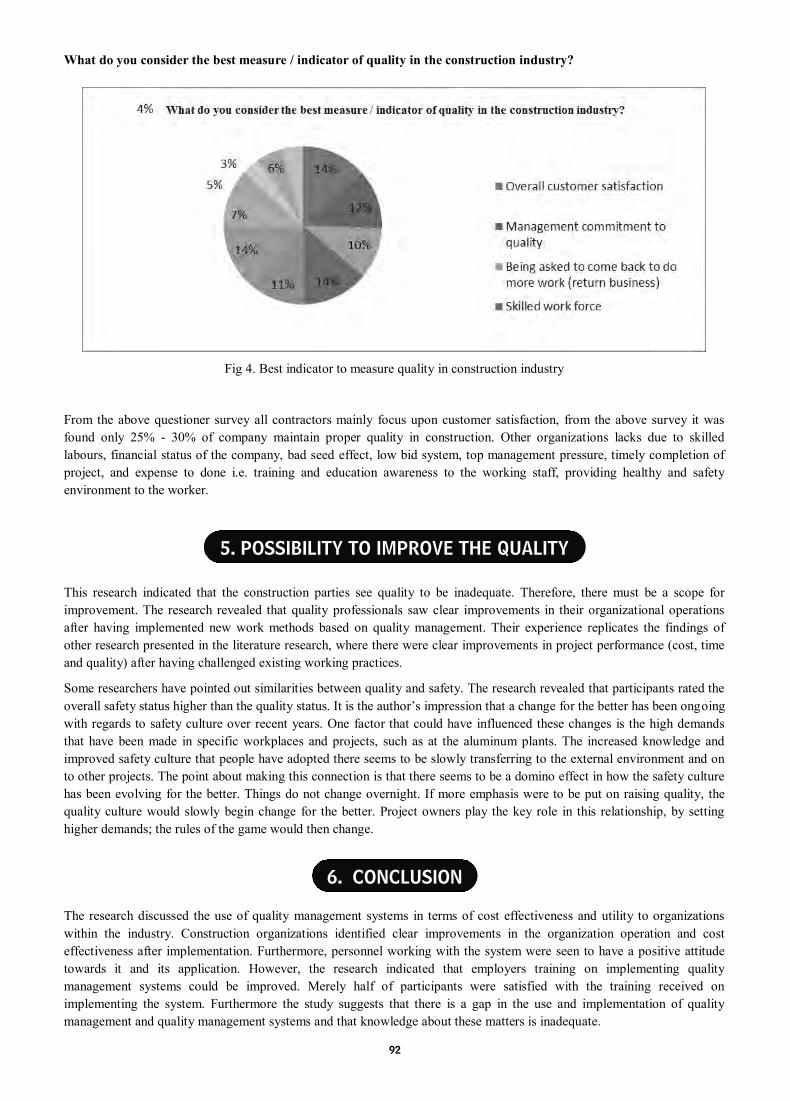
92

What do you consider the best measure / indicator of quality in the construction industry?

Fig 4. Best indicator to measure quality in construction industry

From the above questioner survey all contractors mainly focus upon customer satisfaction, from the above survey it was

found only 25% - 30% of company maintain proper quality in construction. Other organizations lacks due to skilled

labours, financial status of the company, bad seed effect, low bid system, top management pressure, timely completion of

project, and expense to done i.e. training and education awareness to the working staff, providing healthy and safety

environment to the worker.

This research indicated that the construction parties see quality to be inadequate. Therefore, there must be a scope for

improvement. The research revealed that quality professionals saw clear improvements in their organizational operations

after having implemented new work methods based on quality management. Their experience replicates the findings of

other research presented in the literature research, where there were clear improvements in project performance (cost, time

and quality) after having challenged existing working practices.

Some researchers have pointed out similarities between quality and safety. The research revealed that participants rated the

overall safety status higher than the quality status. It is the author’s impression that a change for the better has been ongoing

with regards to safety culture over recent years. One factor that could have influenced these changes is the high demands

that have been made in specific workplaces and projects, such as at the aluminum plants. The increased knowledge and

improved safety culture that people have adopted there seems to be slowly transferring to the external environment and on

to other projects. The point about making this connection is that there seems to be a domino effect in how the safety culture

has been evolving for the better. Things do not change overnight. If more emphasis were to be put on raising quality, the

quality culture would slowly begin change for the better. Project owners play the key role in this relationship, by setting

higher demands; the rules of the game would then change.

The research discussed the use of quality management systems in terms of cost effectiveness and utility to organizations

within the industry. Construction organizations identified clear improvements in the organization operation and cost

effectiveness after implementation. Furthermore, personnel working with the system were seen to have a positive attitude

towards it and its application. However, the research indicated that employers training on implementing quality

management systems could be improved. Merely half of participants were satisfied with the training received on

implementing the system. Furthermore the study suggests that there is a gap in the use and implementation of quality

management and quality management systems and that knowledge about these matters is inadequate.

5. POSSIBILITY TO IMPROVE THE QUALITY

6. CONCLUSION

93

The construction jobsite is not only possible but has proven to be a success. Project results show improved cooperation,

resulting in shorter schedules and punch lists. When a positive team attitude is developed, people will try to outdo each

other in meeting customer expectations.

In a competitive market, businesses stay ahead by offering products that are different and /or superior in ways that matter to

customers. Cost effectiveness has positioned itself at the top end of the modular buildings market in terms of quality, whilst

at the same time providing value-for-money products that fully meet key standards set out in IS0 9001. The company

should meet the required standards in all aspects of quality. This outcome is the result of a great deal of thought, careful

planning and ongoing education and training of a skilled and dedicated workforce.

1. Abdul-Aziz A. Bubshait, Iso 9000 Quality Standards In Construction The Journal Of Management In Engineering,

Vol. 15, No. 6, November/December, 1999.

2. Albert P. C. Chan Factors Affecting The Success Of A Construction Project The Journal Of Construction

Engineering And Management, Vol. 130, No. 1, February 1, 2004.

3. Alexander Laufer, Factors Affecting Construction-Planning Outcomes The Journal Of Construction Engineering

And Management, Vol. 116, No. 1, March, 1990.

4. Amirhosein Jafari Quality Costs In Construction: Case Of Qom Monorail Project In Iran The Journal Of

Construction Engineering And Management, Vol. 139, No. 9, September 1, 2013.

5. Barbara C. Lippiatt Selecting Cost-Effective Green Building Products: Bees Approach Of The Journal Of

Construction Engineering And Management, Vol. 125, No. 6, November/December, 1999.

6. Burcu Aklnci Factors Affecting Contractors' Risk Of Cost Overburden And Possible Publication On August 23,

1996. This Paper Is Part Of The Journal 0/ Ma1lqgement In Engineering, Vol. 14, No.1, January L February, 1998.

7. Harvey A. Kagan, Practical Quality-Controlled Construction The Journal Of Performance Of Constructed Facilities,

Vol. 3, No. 3, August, 1989.

REFERENCES

94

ABSTRACT

COMPARISON OF EXISTING AND PREDICTED SOLID WASTE MANAGEMENT IN AN URBAN

AREA

Adarsh S Faculty of Civil Engineering Department




Tel. No.9538438191,

[email protected]

Shesha Prakash M N Vice Principal, Professor and Head of Civil Engineering Department




Tel. No. 9740011400,

[email protected]

Aishwarya M and Roshan Former Final year students

Department of Civil Engineering




The rising pressure of population together with the constantly changing technologies and development has contributed to

the ever increasing volume of wastes in different forms. Unhygienic environment and solid waste accumulation coincides

with mosquito breeding which causes, the spread of most epidemics. The best example is the present rampant spread of

Dengue and Viral fever across Mysuru. As an environmental package, the disposal of varied solid waste generated from

different sources, such as household markets, commercial areas, slaughter houses, hospitals and industries, makes it more

difficult and challenging. In the present work, Mysuru city has been considered as the study area which has been declared as

one of the smart cities in India. It was seen that during the year 2017, Mysuru city (Karnataka, India) alone contributed

around 402 MT/Day of solid waste from the present population of 9, 38,386 lakhs. The Mysuru City Corporation is

responsible for 65 wards which have set up 9 major solid waste collection units where the waste gets segregated based on

the material and recycling of some of the plastics. The aim of this work is to highlight the importance of zero waste

management and to bring in-sustainability aspects relating to waste disposal. As a result, the present study is aligned with

treating the issues related to waste management in the city along with understanding the present scenario and prediction of

quantity of waste that could be generated in future years which pose a serious threat to our society and eco-system. The



95

future population for two decades (based on 2011 population census) has been predicted by means of arithmetic increase

method and its subsequent solid waste that would be generated has been estimated analytically. The results have shown that

by the end of 2021, the population will be 10, 36, 755 lakhs with 451.11MT/Day of solid waste generated and by the end of

2031, around 519.147MT/Day of waste would be generated for a population of 11, 79,909 lakhs. An action plan has been

devised to mitigate this serious issue which consists of 2 or 3 compost plant of each 200 tons per day capacity and 6 to 8

Biogas plants of capacity 1 ton per day in Zero waste Management.

Keywords: Solid Waste Management (SWM) Municipal solid waste (MSW), Mysuru city cooperation (MCC),

Metric ton (MT)

Increasing population levels, booming economy, rapid urbanization and the rise in community living standards have greatly

accelerated the municipal solid waste (MSW) generation rate in developing countries `(Innocent Ndoh Mbue.,et.al. 2015).

Solid waste is defined as the organic and inorganic waste substances produced through the various societal activities and

have lost value to the first user. Municipal Solid Wastes (MSW) is the commercial and residential wastes produced at the

municipal level or a notified area. The waste could either be in solid or semi-solid form and excludes industrial hazardous

wastes but includes treated bio-medical waste products (Murali Krishna Gurram.,et.al. 2014).

Solid waste generation rate is affected by variety of factors including the geographical location, season, use of kitchen food

waste grinders, collection frequency, characteristics of service area, onsite processing, peoples food habits, economic

conditions, recovery and reuse boundaries, existence of solid waste management laws, local culture and benefits, population

growth, weather conditions and household size (Sama azadi., et.al. 2016).

Solid waste management is an integral part of urban and environmental management, like most of other infrastructural

services has come under great stress, consider low priority areas, solid waste management has never been taken up seriously

either by public or by concerned agency or authorities and now the piled up waste is threatening our heath, environment and

well-being (Vipin Upadhyay et.al. 2012)

The disposal of solid waste is becoming a severe and costly logistical problem in many Asian countries. In most cities of

developing countries, municipal solid waste management costs consume 20-50% of municipal revenues yet collection

service levels remain low with only 5 to 70% of residents receiving service and most disposal being unsafe Municipal Solid

Waste Management (MSWM) of developing countries have typical problem areas such as inadequate service coverage and

operational inefficiencies of services, limited utilization of recycling activities, inadequate landfill disposal and inadequate

management of hazardous and healthcare waste. Solid waste is regarded as one of the most adverse forms of pollution it

requires environmentally sustainable solutions to reduce overall environmental burdens (Muzafar Ahmad Wani.et.al.,

2013).

In order to plan, manage and use municipal solid waste (MSW) in a sustainable way the accurate forecasting of MSW

generation and composition plays a key role in MSW management. Failure of accurate forecasting and assessment may

cause several problems in the environment and waste management systems such as increased environmental impacts and

over-or under-estimated capacity of MSW treatment facilities (Rotchana Intharathirat.et.al.,2014).

Mysore presently known as Mysuru is the third largest city in the state of Karnataka, India, which served as the capital city

of Mysore Princely kingdom (kingdom of Mysore). According to the provisional results of the 2016 National Census of

India, the population of Mysuru is 9, 38,386 and it is spread over an area of 128.42 km2. Mysuru City Corporation is

responsible for the civic administration of the city, which is also the headquarters of the Mysuru district and the Mysuru

division (Adarsh S, et.al. 2017).

The Mysuru municipality was established in 1888 and the city was divided into eight wards. In 1897 an outbreak of

bubonic plague killed nearly half of the population of the city and this paved the way for the establishment of the City

1. INTRODUCTION

2. DESCRIPTION OF STUDY AREA

96

Improvement Trust Board (CITB) in 1903. Mysuru became one of the first cities in Asia to undertake a planned

development of the city. At present, the city is divided into 65 wards. Mysuru city status in terms of population and few

other important features is given below in Table 2.1.

Table 2.1: Mysuru City profile

Municipal Solid Waste Management involves interplay of seven functional elements, namely generation of waste,

segregation, storage, collection, transport, processing and recovery and disposal (Swapan Das., et.al. 2014). It encompasses

planning, organization, administration, financial, legal and technological aspects involving interdisciplinary relationships.

Mysuru Municipal Corporation also performs the same procedure of MSWM in an attempt to minimize the health,

environmental and aesthetic impacts of solid wastes in the city. MCC is responsible for the management of solid waste

generated in the city. The city administration has been decentralized into 9 zones which includes all 65 wards in the city, as

shown in table 3.1. The chief Health Officer of each zone is the overall in-charge of solid waste management in the

corresponding zone of the city.

Table 3.1: Wards distribution Zone Wise.

According to MMC, around 402 TPD solid waste is collected every day in Mysuru city. Waste was being transported each

day which comprised fresh as well as old waste of backlog. Below Table 3.2 shows the waste generation, population,

commercial establishments, educational institution, hotel and waste collected zone wise, finally table 3.3 shows the total

quantity of waste generated in Mysuru City.

FEATURES STATUS

Population 9,38,386

Households 2,06,372

No. of municipal corporation wards 65

Area within corporation limit 128.42 km2

Height above mean sea level(MSL) 770 m

Annual rain fall 798.2 mm

Total waste generated (exiting) 402 MT/day Latitude & Longitude 12o 18’ 12” N, 76o 38’ 45” E

3. REVIEW OF EXISTING SCENARIO

ZONES WARDS

Zone 1- Vidhyaranyapuram 6 (1,2,3,4,5,6)

Zone 2- Jayanagara 8 (7,8,9,10,11,12,13,14)

Zone 3- Mysuru University 9(15,16,17,18,19,20,21,22,24)

Zone 4- Gokulam 5 (23,30,31,32,33)

Zone 5- Kumbarakoppalu 5 (25, 26,27,28,29)

Zone 6- Jodi tengina Mara Burrial Ground 5 (34,35,36,37,38)

Zone 7- Jodi tengina Mara Burrial Ground 8 ( 39,40,41,42,43,44,45,64)

Zone 8- Old Kesare 9 (46,47,48,49,50,51,52,53,54)

Zone 9- New keasare 10 (55,56,57,58,59,60,61,62,63,65)

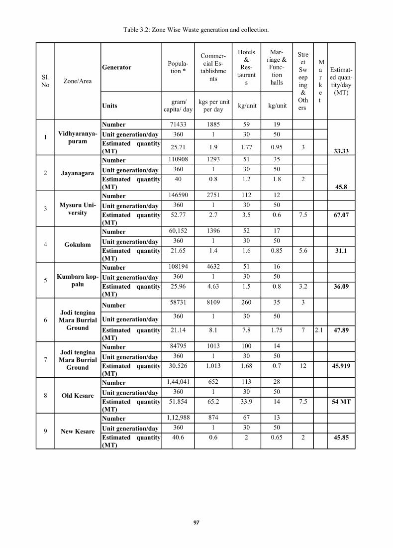
97

Table 3.2: Zone Wise Waste generation and collection.

Sl.

No Zone/Area

Generator Popula-

tion *

Commer-

cial Es-

tablishme

nts

Hotels

&

Res-

taurant

s

Mar-

riage &

Func-

tion

halls

Stre

et

Sw

eep

ing

&

Oth

ers

M

a

r

k

e

t

Estimat-

ed quan-

tity/day

(MT)

Units gram/

capita/ day kgs per unit

per day kg/unit kg/unit

1 Vidhyaranya-

puram

Number 71433 1885 59 19

33.33

Unit generation/day 360 1 30 50

Estimated quantity

(MT) 25.71 1.9 1.77 0.95 3

2 Jayanagara

Number 110908 1293 51 35

45.8


Estimated quantity

(MT) 40 0.8 1.2 1.8 2

3 Mysuru Uni-

versity

Number 146590 2751 112 12


Estimated quantity

(MT) 52.77 2.7 3.5 0.6 7.5 67.07

4 Gokulam

Number 60,152 1396 52 17


Estimated quantity

(MT) 21.65 1.4 1.6 0.85 5.6 31.1

5 Kumbara kop-

palu

Number 108194 4632 51 16


Estimated quantity

(MT) 25.96 4.63 1.5 0.8 3.2 36.09

6 Jodi tengina

Mara Burrial

Ground

Number 58731 8109 260 35 3


Estimated quantity

(MT) 21.14 8.1 7.8 1.75 7 2.1 47.89

7 Jodi tengina

Mara Burrial

Ground

Number 84795 1013 100 14


Estimated quantity

(MT) 30.526 1.013 1.68 0.7 12 45.919

8 Old Kesare

Number 1,44,041 652 113 28


Estimated quantity

(MT) 51.854 65.2 33.9 14 7.5

54 MT

9 New Kesare

Number 1,12,988 874 67 13


Estimated quantity

(MT) 40.6 0.6 2 0.65 2

45.85

98

Table 3.3: Waste Generation Details of Mysuru city.

Quantity and characteristics of the waste are the major factors, which decide technology to be used for waste disposal. On

the basis of the waste quantity, infrastructure requirement can be estimated. It is also necessary to carry out waste analysis

frequently in order to assess the changes in waste characteristics due to ever-changing scenario. This data will also serve as

a basis for up gradation or switching over to better disposal/treatment option (Swapan Das., et.al. 2014).

Storage of waste at source is the first essential step of Solid Waste Management without affecting health and hygiene of

population in the surrounding area. Every household, shop and establishment generates solid waste on day to day basis. The

waste should normally be stored at the source of waste generation till collected for its disposal.

The future amounts of waste are closely coupled to economic growth given un-changed waste intensities in economic and

human activities. Again the waste generation is directly proportional to the rate of change of population. A mathematical

calculation is ultra process beginnings with the estimation of future population based on the average increase in population

of last two decades and then calculate the future amount of municipal solid waste generation as below.

4.1 Arithmetical increase method (AIM)

Future Population, Pn= P + n I

Where, Pn = future population at nth decade

P = Present population

I = average population increase in the known decade

n = no. of decades between now and future

4.2 Calculation of solid waste generated for future years

Quantity, Wq = Pn x W r / 1000

Here,

Pn = Predicted population, and

Wr = Waste generation Rate (kg/capita/day).

The quantity of municipal waste generation will be in metric tonnes. The future population and waste generation is

calculated from the formulation taken 2011 as a base year are shown in table 5.1. Calculation of predicted population and

predicted solid waste quantity for the year 2021 and 2031 is given below.

Sl. No

Generator Number

Unit generation per day

Estimated

quantity/day (MT)

1 Population 9,38,386 360 gram/capita/day 338

2 Commercial establishments 20,329 1.0 kg/unit/day 20

3 Hotels and Restaurant 716 30 kg/unit 21

4 Marriage and function hall 127 50 kg/unit 6

5 Street sweeping 17

Total MSW generated/day in MT 402 MT

4. METHODOLOGY


99

5.1 Population determination using AIM

Total Increase = 286307

I = 286307/2 = 143153

P2021 = P + n x I

P2021 = 893062 + 1x143153

P2021 = 10, 36, 755

P2031 = 893062 + 2x143153

P2031 = 11, 79,909

5.2 Total solid waste generation for future years per day (2021)

Population = 10,36,755 x 360 gram/capita/day = 373.23 MT

Commercial establishment = 22587 x 1 kg per unit per day = 22.587 MT

Hotels and restaurants = 1060 x 30 kg/unit = 31.80 MT

Marriage and function = 170 x 50 kg/unit = 8.5 MT

Street sweeping = 23 MT

Total waste generated per day = 451.11MT

5.3 Total solid waste generation for future years per day (2031)

Population=11,79,909*360 gram/capita/day = 424.76 MT

Commercial establishment = 25015*1kgs per unit per day = 25.587 MT

Hotels and restaurants = 1300*30 kg/unit = 31.80 MT

Marriage and function = 200*50 kg/unit = 10 MT

Street sweeping = 27 MT

Total waste generated per day = 519.147 MT

Table 5.1: Population and Waste Generation Projection of Mysuru City upto Design Year 2031

Projections for urban municipal solid waste generation in 2031 are made by factoring expected growth in population and

estimated per capita waste generation. The population data collected from census conducted by Government of India as per

the report of technical group on population projections constituted by the national commission on population to the office of

the Registrar general & Census commissioner of India. The population projection is calculated by forecasting method. The

population growth in Mysuru from 2011 to 2031 shall have a growth of 25% in 20 years at a rate of 1.2% of annum. This

growth rate is considered in the model from 2011 to 2031 to predict the MSW generation. The MSW data collected from

Year Population Waste generation Quantity (MTD)

% increase in

Population % increase in

Waste generation

1991 606755 330.35 - -

2001 755379 365.25 24.5 10.6

2011 893062 400.15 18.2 9.6

2021 1036755 451.11 16.1 12.7

2031 1179909 519.147 13.8 15.1

100

MCC as per the office records and survey work. It is estimated that the amount of waste generated in Mysuru will increase

at a per capita rate of approximately 1.2% annually is considered for estimate of MSW from the year 2011 to 2031. The

population versus increase of municipal solid waste generation of year wise from 1991 to 2031 is obtained from forecasting

method shown below in Fig. 5.1.

Fig. 5.1 Population and MSW generation projection in Mysuru.

From Fig. 5.2, it is seen that the percentage increase in population is inversely proportional to the percentage increase in

waste generation. Even though there is a decrease in the increasing trend of population, the waste generation has an

increasing trend in percentage increase for different decades.

Fig. 5.2 Decade-wise percentage variation of population and waste generation

5.4 Existing SWM in Mysuru The waste arising from Residence, Hotels, Markets, Drain silt and Slaughter house is

first segregated at the source point as wet waste and dry waste. The segregated waste is then collected through door to door

service by auto or tippers provided by MCC. The collected primary waste is then sent to zero waste management unit. The

management unit motivates the redesign of resource life cycles so that all products are reused which is called as secondary

segregation. After the segregation process, wet waste is sent to composting unit in Mysuru, 200 ton capacity compost plant

located near Vidyaranyapuram. Here 50% of the waste is land filled and remaining waste is composted to produce manure

and sold to market. Dry waste is segregated in 11 categories and sold to the reprocessors to recycle and reuse. Presently, out

of 402 MT generated in Mysuru city 200 MT is sent to a composting unit to produce a manure, 80 MT waste is sent to

ZWM unit where secondary segregation is done which is the next step for recycle and reuse, 6 MT of slaughter house waste

101

is incinerated through pyrolysis process, remaining 6 MT waste is dumped into a biogas plant located at the ZWM unit to

produce a compressed natural gas (CNG). Remaining 100 MT of solid waste is dumped open land, in the mean time MCC

has proposed to setup 2 Compost plant at Rayanakere & Old Kesare of 200 TPD each for future waste generation. Figure

5.2 shows the existing SWM process flow sheet in Mysuru city.

Fig 5.2: Flow sheet of Existing SWM in Mysuru

5.5 Proposed Action Plan of Predicted SWM The predicted solid waste by the end of the year 2031 is around 519.147

MT for which a necessary action plan is as follows.

To treat the predicted solid waste, it is proposed to setup 1 new compost plant of 200 MT at Rayanakere or Old Kesare

immediately. Where MCC has already proposed to setup 2 compost units to treat the excess waste.

Presently there are 6 Biogas plant of capacity 1 MT each in ZWM Plants which can extend to install 3 more Biogas

plant of 1 MT capacity.

Incineration unit needs to be elaborated by installing extra Pyrolysis unit to treat extra 14 MT capacity of slaughter

house waste.

Fig 5.3 shows the flow sheet of proposed action plan of predicted solid waste management

Fig 5.3: Flow Sheet of Proposed Action Plan of Predicted SWM.

Predicted Solid waste

for the Year 2031 is

519.147 MT

Composting plant-

400 MT

ZWM- 90 MT (9

units of 10 MT

capacity each)

Non- Vegetarian

waste- 20 MT

9 Biogas Units at

ZWM Plants (1 MT

capacity each)

Land fill- 200 MT

Composting -200 MT

102

This research work consists of essential findings that have implications for solid waste management. As a case study, the

study area has been chosen as Mysuru city which has adopted an effective solid waste management system which includes

proper collection, segregation, transportation and disposal of waste. The scope of future waste generation is analysed by

forecasting method and illustration of the estimates of waste quantum for period from 2011 to 2031 is presented. The

estimates show that, with the population growth, the percentage increase in per capita waste generation rate will be increase

proportionally. The result shows that the expected municipal solid waste generation by Mysuru city in 2031 is 519.147

Metric tones. With rapid development of economy and change of living standard, waste composition is expected to change.

For a decoupling to take place between economic growth and waste generation, the waste generation by firms and

households in relation to their economic activities must decrease in the future. A number of studies have found that the

higher the household income and standard of living, the higher the amount of MSW generated. The per capita waste

generation rate is changing from decade to decade, due to change in economic growth. The present study also indicate that

much larger land area need to be used for land filling and composting, because the municipal solid waste generation will be

increased in the coming decades, where the initiative is already taken by MCC. The biodegradable waste can be processed

by aerobic composting, which is already in progress in Mysuru city, MCC is working on other techniques like vermi-

composting, anaerobic digestion or any other appropriate biological processing for stabilization of waste.

1. Adarsh S, Shesha Prakash M N (2017) “A Comprehensive Study on Existing Solid Waste Management in Mysuru

City”. International Journal of Engineering, Sciences and Management, 7(1), pp. 23-36.

2. Innocent Ndoh Mbue, Bitondo D, Balgah Roland Azibo (2015) “Municipal solid waste generation, composition,

and management in the Douala municipality”, Cameroon. Journal of Environment and Waste Management, 2(4),

pp. 91-101.

3. Muzafar Ahmad Wani and Shamim Ahmad (2013) “Challenges, Issues of Solid Waste Management in Himalayas:

A Case Study of Srinagar City”. African Journal of Basic & Applied Sciences 5 (1) pp.25-29.

4. Rotchana Intharathirat, P. Abdul Salam (2014) “Uncertainty of Forecasting of Municipal Solid Waste Generation

and Composition: A Case Study of Thailand”. EurAsia Waste Management Symposium, 28-30 April 2014, YTU

2010 Congress Center, Istanbul/Turkiye.

5. Sama azadi, Ayoub karimi-Jashni (2016) “Verifying the performance of artificial regression in predicting the mean

seasonal municipal solid waste generation rate: A case study for fars province, Iran”. Journal of waste management

pp. 14-23.

6. Swapan Das and Bidyut Kr. Bhattacharyya (2014) “Estimation of Municipal Solid Waste Generation and Future

Trends in Greater Metropolitan Regions of Kolkata, India”. Journal of Industrial Engineering and Management

Innovation 1(1) pp. 31-38.

7. Vipin Upadhyay, Jethoo A.S, Poonia M. P (2012) “Solid Waste Collection and Segregation: A Case Study of MNIT

Campus, Jaipur”. International Journal of Engineering and Innovative Technology (IJEIT) 1(3), ISSN: 2277-3754.

8. Murali Krishna Gurram, Lakshmana Deekshatulu Bulusu and Nooka Ratnam Kinthada (2014) “An Appraisal of

Sustainability Scenario of Solid Waste Management: A GIS Study on Municipal Wards of Hyderabad, India”. J

Geol Geosci, an open access journal 3(2) pp. 1-5.

6. CONCLUSION

REFERENCES

103

1. SCOPE OF THE JOURNAL

2. RPOSE OF HE JOURNAL

3. AIM OF THE JOURNAL

4. GUIDELINES FOR AUTHORS

INTERNATIONAL OF SCIENCES AND MANAGEMENT (ISSN:

International Journal of Engineering, Sciences and Management is a bi-annual

journal of Dronacharya Group of Institutions, Greater Noida, UP, India.

To publish full-length research papers in any one or more of the following disciplines:

Computer Science & Engineering, Information Technology, Electrical, Electronics &

Communication Engineering, Mechanical Engineering, Civil Engineering, Physics, Mathematics,

Economics, and Management.

To keep the academic community abreast of the research and technical scenario in the stated

disciplines in the world.

3. A

The aim of the Journal is to percolate latest information in the fields of Engineering, Technology and

Management to aspiring minds to carryout meaningful research work and thereby benefit mankind in

all possible ways. Knowledge shared on this common platform will immensely help researchers for

gainful outputs.

.

SUBMISSION OF MANUSCRIPTS: Soft copy of the manuscript for consideration of publication should be sent (as MS

Word Windows 2007 attachment) by Email to the Executive Editor at advisor.r&[email protected]

PREPARATION OF MANUSCRIPTS:

Manuscript: Manuscript should be in English, the preferred spelling being that of the Concise Oxford

Dictionary. It should be in ‘Times New Roman’, single-spaced, and typed on 8.5" x 11" or A4-size paper with

margins of 1" (25 mm) on each side. Manuscript should be typed in single column only (and not in double or triple

columns).

Title of Paper: Font size 16, ALL CAPITALS, bold, centered, and not underlined. The title must be 12.5 mm

below the top of the page (in addition to the standard 25 mm margin). The Title should adequately describe the

contents of the paper

Full names of all Authors, with * as superscript with corresponding author's name and his/her Email ID

(Font size 12, centered) and also the contact number. A blank line should be left between the title and the author's

name(s).

Full postal address along with affiliations (Font size 10, centered).

mailto:advisor.r%[email protected]

104

Abstract (Font size 10, centered) All papers must have a non-mathematical abstract of not more than 200 words.

The abstract should indicate the general scope of the paper, the important findings and the conclusions drawn.

The abstract should include only text. It should be specific about the methodologies used and the conclusion

drawn of the work reported. Please avoid the use of abbreviations and references. (Text of the Abstract: Font

size 9, single-space, justified).

Keywords: Include up to six keywords that describe your paper for indexing and for web searches. The more

discriminating your keywords are, the greater is the likelihood that your article will be found and cited. (Font size 9,

italics, left-justified).

Text: (Font size 10, Justified). The paper must be divided into sections starting preferably with "Introduction"

and ending with ''Conclusion". The main sections should be numbered 1,

2, 3 etc and subsections as 2.1, 2.2 etc. Main headings should be typed in capitals, subheadings in lower case. Both

types of heading should be underlined and left-justified. Footnotes should be avoided. Equations should be

typewritten and with the equation number placed in parentheses at the right margin. Reference to the equation should

use the form 'Eq. (3)'. Use extra line spacing between equations, illustrations, figures and tables. The use of SI units

is strongly recommended

Tables and Figures: Tables and Figures should be integrated with the text (and not sent separately at the end

of the manuscript) and numbered consecutively in the order in which

reference is made to them in the text of the paper. All captions must be centrally located above a Table and

below a Figure (Font size 10). All tables and figures must be numbered consecutively in Arabic numerals (not

Roman) (e.g., Table 3 or Fig. 3) in the order of appearance in the text. Tables & Figures should be reproduced in the

exact format and at the exact place as desired to appear in the journal.

Conclusion: A conclusion section must be included and should indicate clearly the advantages,

limitations and possible applications of the paper. Authors may also discuss about the scope of future work.

Acknowledgements: An acknowledgement section may be included after the ‘Conclusion’.

References: It is mandatory for references to be quoted in the text and be placed at the end of the text. They should

be numbered consecutively in order of their citation in the text and be indicated by superscripts in the text of the

manuscript. Examples of different citations as References are given below:

(i) In case of referring to an Article in a Journal

Kuebel, D.; Lahiri, M. & Wolf, E. An Inverse Problem in the Theory of Stochastic Electromagnetic Beams, Opt.

Commn., 282, 2009, p.141.

(ii) In case of referring to a Book/Monograph

Rao, C.N.R. & Raveau, B. (Eds.). Transition Metal Oxides, Wiley-VCH, 2nd Edition, 1998, Ch. 2.

(iii) In case of referring to a Conference Paper

Ctvrtnickova, T.; Mateo, M; Yanez, A. & Nicolas, G. Characterization of Coal Fly Ash Components by Laser-

Induced Breakdown Spectroscopy. Presented at the Fifth International Conf. on Laser-Induced Breakdown

Spectroscopy, Berlin, Adlershof, Germany. Sep 22-26, 2008, CP-15, p. 67-68.

(iv) In case of referring to a Report

Marine, R.E. & Iliff, K.W. Application of Parameter Estimation to Aircraft Stability and Control. NASA, USA,

1986, Report No. NASA-RP-1168.

105

Papers quoting the LATEST references from the referred journals will be preferred for publication unless the

original contribution from the author/s is of a very high standard.

Authors must include in the covering e-mail that their paper has not been published/accepted/submitted for publication/

presentation to any other journal/ book/conference in any form and the work submitted by them is their own and original.

The same ‘Undertaking’ should also be attached, on a separate page, along with the manuscript. This ethical policy of the

Journal will be strictly adhered to.

Note: Manuscripts not in conformity with these ‘Guidelines’ will not be forwarded to the

experts for review.

UNDERTAKING

ISSN No. 2231-3273

INTERNATIONAL JOURNAL OFENGINEERING SCIENCES AND MANAGEMENT

Vol. VII | Issue II | Jul - Dec 2017

Dr. Kripa Shankar

Professor, IIT Kanpur, India

(Former Vice Chancellor, UPTU)


Mr. Rajiv Khoshoo

Senior Vice President

Siemens PLM Software,

California, USA


Mr. Mayank Saxena

Director, Advisory Services

Price Water House Coopers


Dr. T.S. Srivatsan

Professor,

University of Akron, USA


Dr. Kulwant S Pawar

Professor, University of Nottingham, UK


Dr. Roop L. Mahajan

Lewis A. Hester Chair Professor in Engineering

Director, Institute for Critical Technology &

Applied Science (ICTAS) Virginia Tech, Blacksburg, USA


Dr. A.K. Nath

Professor, IIT Kharagpur, India


Dr. Mrinal Mugdh

Associate Vice President,

(Academic Affairs)

University of Houston,

Clear Lake, Texas, USA


Dr. Shubha Laxmi Kher

Director & Associate Professor,

Arkansas State University, USA


PATRON

Dr. SatishYadav

ChairmanDronacharya Group of Institutions, Greater Noida

EDITOR-IN-CHIEF

Dr. Ashish Soti

DirectorDronacharya Group of Institutions, Greater NoidaE-mail: [email protected]

EXECUTIVE EDITOR

Wg Cdr (Prof) TPN Singh

Advisor (Research & Development)Dronacharya Group of Institutions, Greater NoidaE-mail: advisor.r&[email protected]

EDITORIAL BOARD

Dr. Ganesh Natarajan

Founder - 5F WorldChairman - NASSCOM Foundation & Global Talent TrackPresident - HBS Club of IndiaE-mail: [email protected]

Dr. Satya Pilla

Boeing Space Exploration,iGET Enterprises,Embry-Riddle Aeronautical UniversityE-mail: [email protected]

Dr. R.P. Mohanty

Former Vice ChancellorShiksha 'O' Anusandhan UniversityBhubaneswar, IndiaEmail: [email protected]

Mr. Uday Shankar Akella

Chairman & Managing DirectorRSG Information Systems Pvt LtdHyderabad, IndiaEmail: [email protected]

Dr. Sanjay Kumar

Vice ChancellorITM University ChhatishgarhFormer Principal AdvisorDefence Avionics Research Establishment (DARE)E-mail: [email protected]

BUT WE CAN BUILD OUR YOUTH FOR THE FUTURE

WE CAN NOT ALWAYS BUILD THE FUTURE FOR OUR YOUTH,

GROUP OF INSTITUTIONS

-Franklin D Roosevelt

Here We Build Your Future

B. TECH COURSES| |Computer Science & Engineering Electronics & Communication Engineering Electronics & Computer Engineering

Electrical & Electronics Engineering Mechanical Engineering Computer Science and Information Technology| |

Information Technology Civil Engineering|

POST GRADUATE COURSESMaster of Business Administration (MBA) Master of Computer Application (MCA)|

Campus: #27, Knowledge Park- III, Greater Noida (UP) Phone: 0120-2323851-58, 2322022 | Email: [email protected] India Council for Technical Education, New Delhi (India) Dr. A. P. J. Abdul Kalam Technical University, Lucknow (India)Approved by: | Affiliated To:

DRONACHARYA GROUP OF INSTITUTIONS

Approved by

All India Council for Technical Education, New Delhi (India)

Affiliated To:

Dr. A. P. J. Abdul Kalam Technical University, Lucknow (India)

Campus:

# 27, Knowledge Park-III, Greater Noida (U.P.) – 201308 (India)

Phone: 0120-2323854-58, 2322022, Email: advisor.r&[email protected]

Corporate Office:

76P, Part-III, Sector-5, Gurgaon, 122001, Haryana (India)

Phone: 0124-2251602, 2253144, Email: [email protected]

desi

gn: w

ww

.stu

dio1

-indi

a.co

m

IJESM SIGHTINGS INTERNATIONAL JOURNAL OF

ENGINEERINGSCIENCES AND MANAGEMENT

ISSN No. 2231-3273

www.dronacharya.info


GREATER NOIDA, U.P., INDIAGROUP OF INSTITUTIONS

J O U R N A L M A S T E R L I S T

Vol. VII | Issue II | Jul-Dec 2017

Brazil 3.5%2.3%

India 60.5%

United States 12.6%

139 different countries have visited this site. 189 flags collected.

1.6%

1.1%

1.0%

1.0%

0.9%

0.8%

0.8%

0.7%

0.7%

0.6%

China

Unknown - A/P

Czech Republic

Iran

Indonesia

Malaysia

Nigeria

Pakistan

United Kingdom

Italy

Egypt

Others 11.9%