Embed Size (px)
Citation preview

1
IIMB WORKING PAPER NO.2010-01-301
ECONOMIC DEVELOPMENT, INEQUALITY
AND MALNUTRITION IN INDIA
Arnab Mukherji,
Indian Institute of Management Bangalore
Centre for Public Policy,
Email:[email protected]
Divya Rajaraman,
St. John’s Research Institute
Email:[email protected]
&
Hema Swaminathan
Indian Institute of Management Bangalore
Center for Public Policy,
Email: [email protected]

2
Economic Development, Inequality and Malnutrition in India1
Arnab Mukherji Divya Rajaraman Hema Swaminathan Center for Public Policy,
IIM Bangalore, India
St. John’s Research Institute, AND IIM Bangalore, Bangalore India
Center for Public Policy, IIM Bangalore, India
Abstract
Economic development and inequality is known to have an impact on health
outcomes. We show this to be true in India where we study the effect of economic
status on under and over nutrition. Inequality is measured using income or assets
and we show that both matter for malnutrition. We find women are at much
higher risk of being malnourished and this risk increases with age. Our results
suggest that while under nutrition should remain a policy priority, rising over
nutrition in the population cannot be ignored by nutritional planners.
I. Introduction
An individual’s economic and health status are strongly correlated in both industrialised
and developing societies (Wilkinson, 1998, Thomas and Frankenberg, 2002). The potential
mechanisms through which economic status affects or is affected by health status are many.
However, these mechanisms are only partially understood. The focus of most empirical analyses
on this relationship between income and inequality with health outcomes has largely tended to be
1 We’ like to thank Dr. Ajay Kumar Singla for initial discussion on this topic and to the Public Health
Group at IIM Bangalore for providing a forum for us to interact.

3
on stark health outcomes such as mortality (Deaton, 2003, Wilkinson, 2005, Smith, 1999). Much
less evidence is available on the relationship between economic status, both economic
development and inequality, and malnutrition, a less extreme, but nevertheless potentially
debilitating outcome.
Malnutrition is a state of poor nutrition which includes under nutrition, over nutrition,
and nutrient deficiency Malnutrition imposes significant costs on society; an adult being
underweight often indicates chronic energy deficiency which is associated with reduced physical
work capacity and productivity, and negative pregnancy and maternal health outcomes. Being
underweight is also associated with greater risk of morbidity and mortality (Shetty and James,
1994). Overweight and obesity are risk factors for cardiovascular disease, type 2 diabetes,
several cancers, and renal, hepatic and respiratory related mortality. Obesity is also associated
with depression (Haslam and James, 2005, Whitlock et al., 2009). Thus, from a policy
perspective, it is important to understand the prevalence and distribution of malnutrition in a
society, in order to make decisions about how to direct resources to prevent and mitigate the
associated burden of disease.
In the past fifty years, there have been huge shifts in the global distribution of
malnutrition. Different societies are at different stages of ‘nutrition transition’; this is a process
of changes in the food-diet environment, physical activity and lifestyle that result in shifts in
nutritional status at the population level, with average Body Mass Index generally rising over
time (Caballero and Popkin, 2002). Because these factors are strongly linked to individual and
societal economic status, high income countries are expected to be further along on the nutrition
transition, with food security and under nutrition being less of a concern than the health and

4
economic costs of over nutrition (Popkin, 2009, Popkin and Gordon-Larsen, 2004, World Health
Organization and Food and Agricultural Organization, 2003).
Low and middle income countries are, however, increasingly experiencing a dual burden
of both under and over nutrition (World Health Organization and Food and Agricultural
Organization, 2003). In developing countries, child and adult under nutrition continue to be a
major health concern, contributing to both morbidity and mortality. In 2005, 17 per cent of
individuals in all developing countries, and 21 per cent of South Asia’s population were
undernourished (United Nations, 2009). At the same time, increasing urbanization, and changes
in diet and lifestyle brought on by globalization and economic development are associated with
rising over nutrition and associated chronic diseases, in some cases at a very rapid rate
(Caballero, 2001, Miranda et al., 2008, Popkin, 2002). The ratio of over to under nutrition in low
income countries is also showing an upward trend. Recent analysis of nutritional data for adult
women from 37 developing countries show that more women were overweight than underweight
in over half the countries (Mendez et al., 2005).
It is well documented that the prevalence of under nutrition in India remains persistently
high (Haddad and Zeitlyn, 2009, Deaton and Dreze, 2008), with the prevalence of under nutrition
amongst adult women in 2005-2006 at 33 per cent, down only 3 percentage points from 36 per
cent in 1998/1999 (IIPS and Macro International, 2007). However, what is less discussed with
regard to India’s malnutrition concerns is the fact that over nutrition and obesity are also on the
rise, from 11 per cent of ever married women in 1998-1999 to 15 per cent in 2005-2006 (IIPS
and Macro International, 2007). This post 1990s decade also coincided with a period of
unprecedented economic growth and prosperity in India leading to increased urbanisation and

5
associated changes in lifestyle choices (Deaton and Kozel, 2005, Mukherji, 2008, Dev and Ravi,
2007). A natural concern that emerges for public policy therefore is the nature of the interactions
between increasing economic prosperity and nutrition transition, and the implications for health
and development policy.
In this paper, using the National Family Health Survey 2005-6 (NFHS-3) data, we
examine the association between various measures of economic development (such as the level
of per capita income, individual wealth, income inequality and wealth inequality), and diet,
activity and lifestyle choices on malnutrition in India. We contribute to the existing literature in
the following ways: a) we model both under nutrition and over nutrition; b) we use a richer set of
state and individual level correlates than have been used in the literature so far and discuss the
role of different forms of economic inequality, and various behavioural variables (such as diet
and activity) that affect nutrition; c) while looking at the role of economic inequality we
explicitly distinguish between wealth and income inequality; and d) we study how these
regression coefficients vary between men and women. We find that economic inequality matters
for both under and overweight, but the effects across different measures of inequality are not similar.
We also find a relatively steady relationship between the regression covariates and malnutrition
across its distribution; thus, variables that reduce under nutrition also tend to increase over
nutrition.
The paper is organised as follows: The next section reviews the literature with a
particular emphasis on the relationships between economic growth, inequality and health.
Section III discusses the data and estimation methodology. The regression results are presented
in Section IV, with policy implications of our findings being discussed in the concluding section.

6
II. Background: Economic Factors Affecting Nutritional Status
Variations in nutritional status between and within countries are associated with both
economic and social indicators. Analysis of the pattern of associations between national income
and malnutrition suggests that over nutrition rises most steeply in middle income countries, and
starts to level off as per capita income rise (Popkin, 2002). As income rises, under nutrition too
tends to decline in general, though more slowly and if these trends continues, the burden of
obesity is likely to systematically shift from higher income countries to low and middle income
countries within the next few years, further increasing existing health inequalities (Ezzati et al.,
2005).
Higher levels of national income are also associated with a changing distribution of
overweight within the country. Analysis of multi-country data on nutritional status suggests that
when a country approaches a GDP of about $2,500 per capita, the burden of overweight starts
shifting from high income groups towards low income groups (Monteiro et al., 2004). The
associations between low socio-economic status (SES) and obesity have been well documented
in high income countries, and causation has been attributed both to material factors such as
access to medical care and environmental exposures, health behaviour and lifestyle, and the
psychosocial and material effects of social and economic inequality (Goodman, 2003). Apart
from average per capita income, the distribution of wealth appears to play a role in prevalence of
malnutrition. In high income countries where obesity is a greater public health concern than
under nutrition, economic inequality is associated with greater prevalence of overweight and
obesity (Pickett et al., 2005). In low income countries, however, there has been limited analysis
of the effects of inequality on malnutrition.

7
The notion that the distribution of income in society, as measured by the variance of
income or Gini coefficient, may have a relationship with health has been debated in the literature
(Deaton, 2003, Wilkinson, 2005). The mechanisms by which inequality in income may affect
individual health are potentially many; models of redistributive politics predict that if a myopic
median voter is making choices in allocation of public goods in more unequal societies, then the
level of health care and education available to society at large will be more sub-optimal for
people at the extremes of the income distribution, the more unequal the initial distribution of
income (Alesina and Rodrik, 1994, Persson and Tabellini, 1994). It has also been argued that the
quality of social relations (such as levels of trust and violence) are better in more egalitarian
societies. Given that low social status and poor social relations are a strong determinant of poor
health, less egalitarian societies are more likely to see poorer health (Subramanian and Kawachi,
2004, Wilkinson, 2005). Indeed, there is an empirically well-documented positive relationship
between inequality and mortality (Wilkinson, 1998).
There already exists evidence that the nutrition transition in India is underway, with
overweight and obesity now a significant public health issue (Griffiths and Bentley, 2001, Siegel
et al., 2008). According to the Nutrition in India report, based on the NFHS-3 data, a significant
number of adults are suffering from both under and over nutrition, with significant regional
variation in the distribution of under and overweight. In five Indian states (Punjab, Kerala, Delhi,
Tamil Nadu and Goa), over 20 per cent of women are overweight, while in another five states
(Bihar, Chattisgarh, Jharkand, Madhya Pradesh and Orissa), more than 40 per cent of women are
underweight (Arnold et al., 2009). Previous analyses of under and overweight in India using data
from 1998-1999 have found individual socioeconomic status to be an important predictor of
being overweight (Griffiths and Bentley, 2001); at the same time, state level economic

8
development increases risk for overweight, while inequality appears to increase the risk for both
under and overweight (Subramanian et al., 2007).
The 1990s have witnessed important changes in the pattern of economic development in
India, with per capita GDP growth averaging 6.5 per cent as opposed to 5.4 per cent in the 1980s.
However, there has been substantial variation in the rate of growth across the different states
(Deaton and Kozel, 2005, Mukherji, 2008, Dev and Ravi, 2007). Moreover, national data reveals
that even in high-performing states, the gains from the high rate of growth of income are not
distribution neutral; in fact, the rate of poverty reduction has stagnated since the 1980s, with
some states actually showing a decline in performance (Dev and Ravi, 2007, Ahluwalia, 2002).
Given the importance that the level of income, its distribution, and other parallel
behavioural changes that accompany economic development, have in determining malnutrition
we exploit the vast cross-sectional variation within India to understand how economic status and
inequality affect health status.
III. Data and Methods
NFHS - 3 is the third in a series of large, nationally representative sample surveys of
households that has been designed to collect information on fertility, infant and child mortality,
the practice of family planning, maternal and child health, reproductive health, nutrition,
anaemia, and utilization and quality of health and family planning services. The first two surveys
(1990-1991 and 1998-1999) collected detailed information on women in the 15-49 years age
groups. The most recent survey additionally included men in 15-54 years age groups. NFHS -3
contains detailed individual, household and community level characteristics that provide height

9
and weight information for individuals, as well as a Body Mass Index (BMI) that is calculated as
weight /height2 (i.e. kg/m
2). BMI is an indicator of nutritional status: a BMI of less than 18.5 is
considered as underweight, while 25-29.9 is overweight and 30 or above is classified as obese
(World Health Organization and Food and Agricultural Organization, 2003). Throughout our
analysis we use two measures of malnutrition; under nutrition when BMI is less than 18.5 and
over nutrition when BMI is 25 or above (including both individuals who are overweight and
obese).
We restrict the NFHS data in two ways to construct our analysis sample: 1) we only
include men and women in the 19-49 age group. We exclude adolescents (18 and under), as it is
not straightforward to classify over and underweight through BMI in this age group. We exclude
men over 50 to ensure comparability of the men and women in the analysis; and, 2) we exclude
currently pregnant women and women who have been pregnant in the last three months as this
affects their body composition. Thus, our analysis sample consists of 101,600 women and 62,013
men in the 19 to 49 age group. We pair the individual-level data with macro-level variables
including state- level per capita income, and state-level Gini coefficients.
Income inequality is captured by state-level Gini coefficients based on household
consumption expenditure calculated by the Planning Commission. In the absence of income data,
we use this as a proxy measure of income inequality. We derive another measure of economic
inequality from the household’s ownership of assets, which is captured by the wealth index in the
NFHS dataset. The wealth index is constructed as a score variable created by conducting a factor
analysis on several asset ownership variables that are a part of the original survey instrument.
While wealth and income are correlated, they capture different economic effects. Wealth is a

10
stock variable representing the currently accumulated value of past income, while income is a
flow variable capturing income flows in the last financial year. Wealth is also considered a more
reliable measure of household welfare than income or consumption, as typically wealth status
does not fluctuate with transitory income shocks. Deininger and Olinto (2000) were amongst the
first to point out that the theoretical literature linking distributional concerns and economic
growth were based on asset inequality, and yet the empirical tests of this prediction used only
income inequality measures. When placing both income inequality and asset inequality in their
growth regressions, they found that asset inequality (with regard to land, which is also a
component of the NFHS-3 wealth index) has a negative effect, while income inequality has a
positive effect.
However, existing empirical evidence on welfare measure also suggests that inequalities
on certain outcomes such as health, education, etc. are largely robust to the measure of economic
status used (Filmer and Scott, 2008). Specifically with respect to child malnutrition, Wagstaff
and Watanabe (2003) find that there is little difference whether one uses household consumption
or a household asset index. In this paper, we use a wealth (asset) inequality index based on
household ownership of assets and an aggregate (state level) income inequality measure. In
addition to capturing inequity in resource distribution, the state level income inequality can serve
as an indicator of social cohesiveness among communities, which can potentially be protective
against malnutrition (Subramanian et al., 2007).
The degree of disaggregation at which one should measure inequality is not obvious.
Mishra and Dilip (2008) have underscored the importance of disaggregating the analysis of
wealth measures in NFHS-3 at the state or the regional level and rural-urban divides within

11
these, to understand the real effects on health outcomes. Thus, we construct two geographical
wealth inequality measures.i The geographical measure of wealth inequality measures the
dispersion in the wealth index (in terms of standard deviations) for households within the same
geographic unit. We consider two geographical aggregations within the state: the standard
deviation of wealth within a state’s urban and rural areas, and the standard deviation of wealth
within each primary sampling unit (PSU) within a state. The dispersion in the wealth index at the
urban-rural level will be greater than the dispersion at the PSU level. This implies that an
individual’s inequality ranking is likely to change as the neighbourhood is defined over a larger
geographic area. Including the two variables separately helps us check the robustness of our
wealth inequality measures as well as empirically testing if the immediate neighbourhood has a
greater impact on an individual’s health. Table 1 presents the correlation coefficients of the
different sources of economic inequality used in the models. If income and assets are distributed
identically in the data then one would expect the correlation to be positive and close to one.
However, we find that not only is the correlation small but it is also negative. This suggests that
the distribution of income and assets in the population are quite different.
The dataset contains dietary information that allows us to examine the relationship
between individuals’ eating habits in the past 30 days, and their nutritional status. Specifically, it
tells us how frequently an individual has been consuming curd, beans, leafy vegetables, fruits,
eggs, meat and fish. For each item, an individual can respond by saying they never consume,
occasionally consume, or consume the particular food item(s) on a weekly or a daily basis. We
classify households into three groups – the strongly non-vegetarian group, that is, those
households who report consuming eggs, and meat, and fish on a weekly or daily basis apart from
other food items during the last thirty days; the vegetarian group, that is, those who report

12
consuming only curd, beans, fruits and leafy vegetables on a weekly or daily in the last thirty
days and finally the mixed diet group, that is, those who consume either eggs, or meat or fish,
but not all of them on a weekly or daily basis in the last 30 days.
Given the binary nature of our outcome variables, we model the relationship between the
likelihood of being obese (or undernourished) as a logistic transformation of a range of state,
community, household, and individual specific covariates. There are a number of advantages to
using a logistic regression to model outcomes that are not continuously observed (in this case
being 1 or 0 to indicate being overweight/underweight or not): specifically, it is possible to
ensure that the relationship between any covariate and the outcome varies across the range of
values that the covariate can take, which would otherwise be constant in an ordinary least
squares regression models (Madalla, 1983). This flexibility also ensures that the interpretation of
the regression coefficients as the ceteris paribus change in probability due to a small change in
the covariate at a specific point in the distribution is consistent and valid, without violating the
natural 0 to 1 range for the outcome variable. Our basic regression model is:
(1)
In the above, i indexes adults in our sample, n indexes the geographical units (depending on the
model, the geographical unit is either the the urban-rural area, or the PSU), and s indexes the
states from which our sample is drawn. is the probability that individual i from
geographical unit n from state s is overweight (or underweight). Inequalityi,n,s is a vector of
measures of economic inequality, both income based (i.e. the Gini coefficient) and asset based
(i.e. the geographical wealth inequality measures at different levels of aggregation). x1,s is a set

13
of state level macro variables that captures the state’s level of economic development, including
per capita income, and level of urbanization. Finally, x2,s is a set of household and individual
specific variables that capture key variables that may affect nutritional morbidity, including
household wealth, age, caste, gender, education, and key variables like diet, and birth history for
women. Interpretation of the regression coefficients (βs) of the regression in equation (1) is in
terms of the change in the log odds of being over (under) weight for a unit change in a covariate.
In our regressions, we report the marginal effect on the probability of being over (under) weight
calculated at the mean of each covariate.
IV. Results
A. Economic Development, Inequality and Malnutrition in India
Figure plots individual wealth index against individual BMI for the entire dataset and
estimates a flexible local linear regression between these two variables to show the association
between wealth index and BMI in the data. It is clear that people with low BMI tend to have a
low wealth index that indicates absence of economic resources while people with high BMI tend
to also have high wealth indices. The diagram also indicates that there is large heterogeneity in
this linear association at each point on the wealth index scale suggesting a potential for a non-
linear relationship between BMI and its determinants when looking at low BMI (under nutrition)
and high BMI (over nutrition).
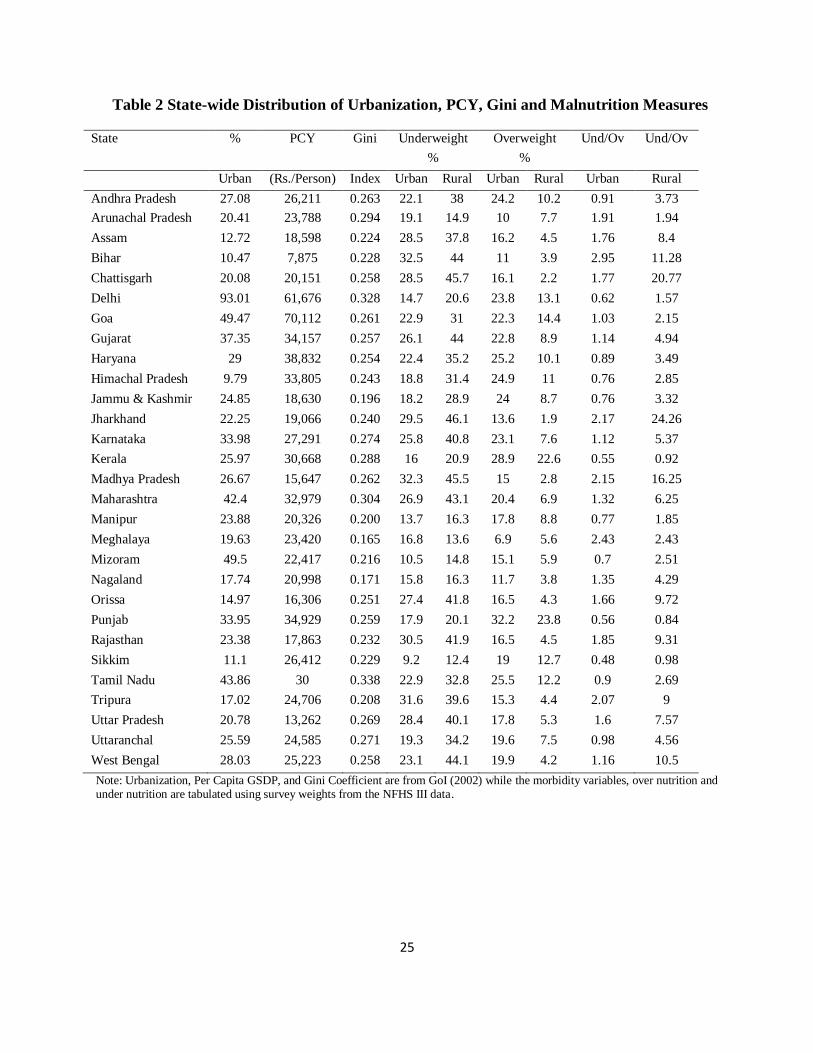
State level urbanization, per capita income (PCY), Gini coefficients and the prevalence of
malnutrition are shown in Table 2. It is noteworthy that there is significant geographic variation
in both economic development and malnutrition. The coefficient of variation, which measures
dispersion of a variable, ranges between 0.15 - 0.65 across these variables.ii The fraction

14
overweight in rural areas has the highest coefficient of variation 0.65, while the Gini coefficient
has the smallest coefficient of variation across states at 0.15-0.16. We exploit this variation in
trying to understand the relationships between economic inequality and malnutrition. The last
two columns report the state level distribution of the ratio of those experiencing under nutrition
to those facing overweight or obesity problems in the urban and rural parts of our sample. The
data suggests that being overweight is largely an urban phenomenon with twelve states showing
greater proportion of population being overweight category as compared being underweight. Of
these, 7 states report in their rural areas, the per cent of population underweight is at least twice
as much as the per cent of population overweight, suggesting a dual burden of malnutrition
overall. What is also surprising is that in rural Kerala, Punjab, and Sikkim, the per cent of
population overweight is greater than the per cent underweight.
Table 3 reports the bivariate correlations between nutritional outcomes and the other state
level variables. We see that income inequality (as measured by the Gini coefficient) is positively
correlated with measures of under and over nutrition and these are statistically significant and
substantively meaningful with large correlation coefficients (greater than 0.30). Being
overweight in either rural or urban areas is positively correlated with state per capita income,
with statistically significant correlation coefficients that are larger than 0.50. Finally, the fraction
of the state that is urbanized is also positively correlated with being overweight; this is
statistically significant, with a coefficient greater than 0.30.
B. Determinants of Over nutrition and Under nutrition
In this section, we present a series of logistic regression models with BMI as the
dependent variable. Our two outcome measures are dummy variables for being under and
overweight; 12 per cent and 33 per cent of the sample are underweight and overweight
15
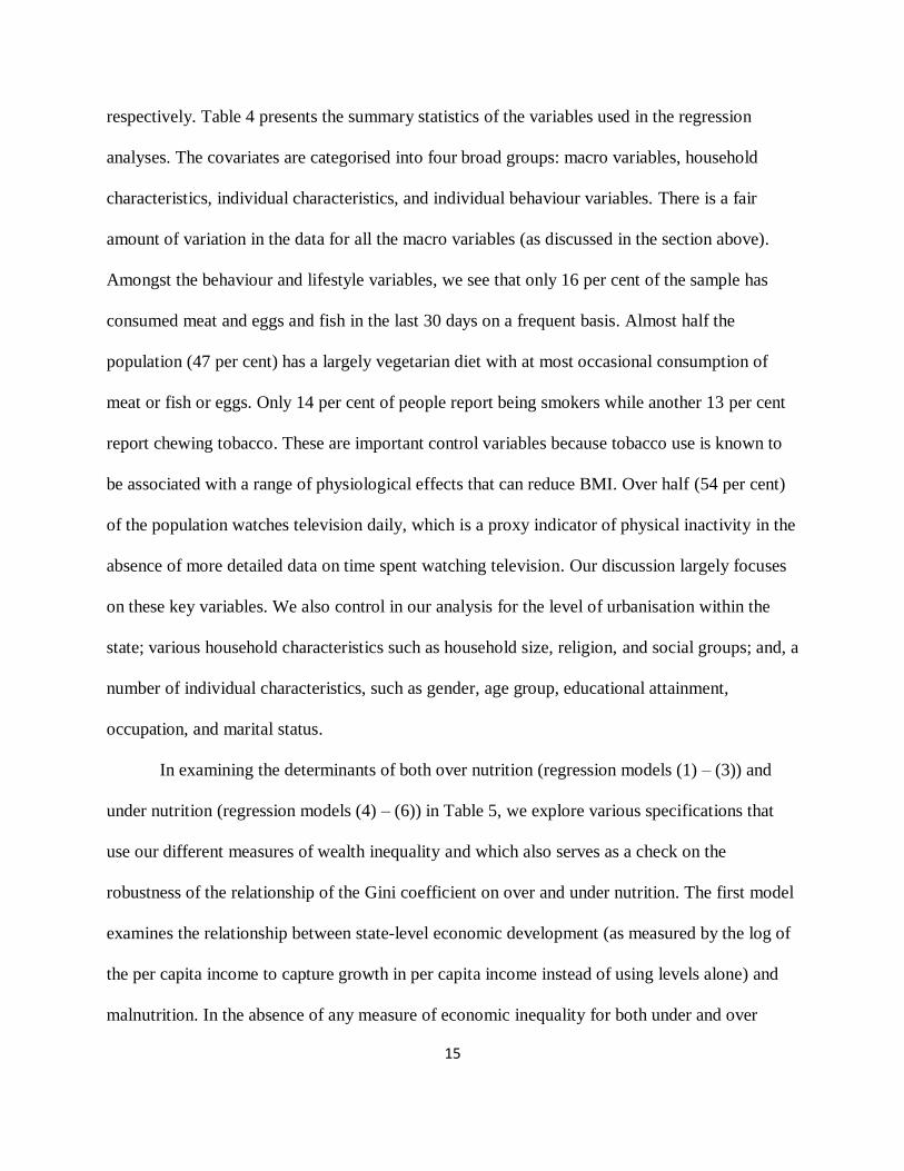
respectively. Table 4 presents the summary statistics of the variables used in the regression
analyses. The covariates are categorised into four broad groups: macro variables, household
characteristics, individual characteristics, and individual behaviour variables. There is a fair
amount of variation in the data for all the macro variables (as discussed in the section above).
Amongst the behaviour and lifestyle variables, we see that only 16 per cent of the sample has
consumed meat and eggs and fish in the last 30 days on a frequent basis. Almost half the
population (47 per cent) has a largely vegetarian diet with at most occasional consumption of
meat or fish or eggs. Only 14 per cent of people report being smokers while another 13 per cent
report chewing tobacco. These are important control variables because tobacco use is known to
be associated with a range of physiological effects that can reduce BMI. Over half (54 per cent)
of the population watches television daily, which is a proxy indicator of physical inactivity in the
absence of more detailed data on time spent watching television. Our discussion largely focuses
on these key variables. We also control in our analysis for the level of urbanisation within the
state; various household characteristics such as household size, religion, and social groups; and, a
number of individual characteristics, such as gender, age group, educational attainment,
occupation, and marital status.
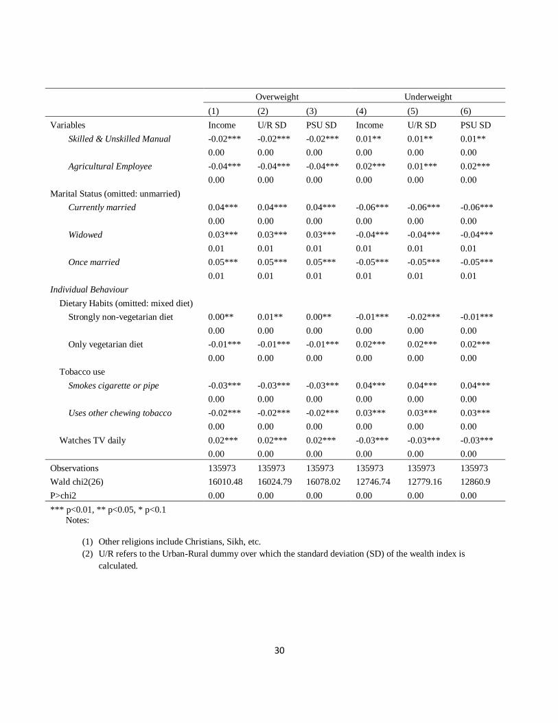
In examining the determinants of both over nutrition (regression models (1) – (3)) and
under nutrition (regression models (4) – (6)) in Table 5, we explore various specifications that
use our different measures of wealth inequality and which also serves as a check on the
robustness of the relationship of the Gini coefficient on over and under nutrition. The first model
examines the relationship between state-level economic development (as measured by the log of
the per capita income to capture growth in per capita income instead of using levels alone) and
malnutrition. In the absence of any measure of economic inequality for both under and over

16
nutrition, there is no effect of the log of per capita income (models (1) and (4), respectively).
However, once we include the income inequality and the urban-rural wealth inequality measure,
we find the log of per capita income decreases the risk of being overweight and increases the risk
of being underweight (models (2) and (5), respectively). This suggests that increasing state level
wealth improves overall nutrition, even after controlling for household wealth. However, the
effect is very small and not robust; a 1 per cent increase in per capita income reduces the
likelihood of being overweight by 0.01 probability point and increases the likelihood of being
underweight by a similar magnitude. Moreover, its effect is not statistically significant once we
include the PSU level wealth inequality as opposed to urban-rural wealth inequality.
The regression results indicate that, apart from state level income, inequality also matters
for both under and over nutrition. However, the effects across the various measures of inequality
are not entirely similar. People living in states with higher income inequality, are both more
likely to be overweight and more likely to be underweight. These results support the findings of
Subramanian et. al’s (2007) analysis of the 1998-1999 NFHS-2 data. In models (1) to (6), 1 per
cent point deterioration in income inequality, as measured on the Gini index, significantly
increases the likelihood of being overweight by a maximum of about 33 per cent points while
reducing the likelihood of being underweight by a maximum of 47 per cent points. This is a large
effect, given that the mean prevalence of being overweight and underweight in the entire
population is about 15 per cent (12.5 per cent for men and 17.2 per cent for women). We find a
similar and stronger relationship between wealth (asset inequality) and under nutrition. Urban-
rural wealth inequality increases the likelihood of being under weight by 9 per cent and the PSU
level wealth inequality by 5 per cent. Surprisingly, the wealth inequality effect on over nutrition

17
is negative and is robust across the geographical units although the effect is quite small, in the
range of 1 – 2 per cent in these models.
The level of urbanisation of the state is statistically significant and positive for all the
overweight models, suggesting that a 1 per cent increase in the level of urbanization will lead to
a two per cent increase in the incidence of overweight. Regressions (4) and (6) suggest that a 1
per cent increase in urbanization is associated with a decline in underweight; however regression
(5), where we control for urban-rural wealth inequality, suggests there is no effect of
urbanization. This might be explained by the rural-urban dummy that could be absorbing
differences between rural-urban areas but is now captured through the wealth inequality
measure. The household-level wealth quintiles also show that households in higher wealth
rankings are at greater risk of being overweight and lower risk of being underweight. These
results are substantiated by another measure of household economic deprivation, having a
‘Below the Poverty Line’ (BPL) card which provides access to state health, food, and education
subsidies.
Diet and other behaviour variables that reflect an individual’s lifestyle also affect
nutritional status. We find that in comparison to those who have had a mixed diet in the past
thirty days with occasional consumption of meat or fish or eggs, high consumption of meat, fish
and eggs increases the likelihood of being overweight and reduces the chances of being
underweight. Conversely, a purely vegetarian diet in the last thirty days reduces the chances of
being overweight and increases the likelihood of being underweight. The effect of nicotine on
BMI is significant and negative with smokers and users of other forms of tobacco at greater risk
of being undernourished and lesser risk of being over nourished. The only measure of physical
activity that was captured in NFHS was watching television frequently. Although it is not an

18
ideal measure given that there is no indication of duration of television watching, the effect is
nevertheless significant, with daily television watching raising the likelihood of being
overweight and reducing the likelihood of being underweight.
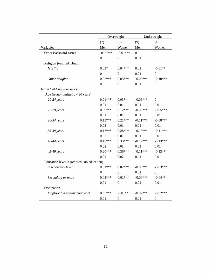
In Table 6, we estimate separate models for men and women to further understand the
differential relationship between the covariates and their nutritional status for men and women.
Focussing mainly on the economic inequality variables, we find that the effects of the Gini
coefficient and the asset inequality are qualitatively similar to the overall models. What is
interesting, however, is that the impact of income inequality increases the risk of being
overweight more for women than men, with the converse being true for the risk of being
underweight. The impact of asset inequality at the PSU level mirrors that of the overall sample; it
reduces the risk of being overweight while increasing the risk of being underweight. Both men
and women are more at risk of being overweight with increasing urbanization. However, only
women are likely to experience a decline in underweight. An interesting finding is that the
likelihood of being overweight is higher for women at all ages, but from age 30 onwards, women
are almost twice as likely as men to be overweight. While diet and behaviour variables tend to
have similar effects for men and women, smoking in women reduces the likelihood of being
overweight and increases the likelihood of being underweight twice as much as it does for men.
V. Discussion
Using individual and macro level data from India, we show that economic status, not only
at the individual and aggregate levels , but also its distribution, i.e. wealth inequality at the PSU
and rural-urban areas, as well as income inequality (the Gini coefficient), is strongly associated
19
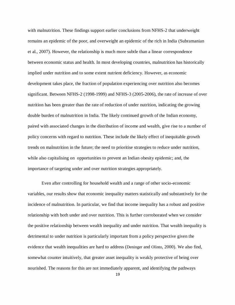
with malnutrition. These findings support earlier conclusions from NFHS-2 that underweight
remains an epidemic of the poor, and overweight an epidemic of the rich in India (Subramanian
et al., 2007). However, the relationship is much more subtle than a linear correspondence
between economic status and health. In most developing countries, malnutrition has historically
implied under nutrition and to some extent nutrient deficiency. However, as economic
development takes place, the fraction of population experiencing over nutrition also becomes
significant. Between NFHS-2 (1998-1999) and NFHS-3 (2005-2006), the rate of increase of over
nutrition has been greater than the rate of reduction of under nutrition, indicating the growing
double burden of malnutrition in India. The likely continued growth of the Indian economy,
paired with associated changes in the distribution of income and wealth, give rise to a number of
policy concerns with regard to nutrition. These include the likely effect of inequitable growth
trends on malnutrition in the future; the need to prioritise strategies to reduce under nutrition,
while also capitalising on opportunities to prevent an Indian obesity epidemic; and, the
importance of targeting under and over nutrition strategies appropriately.
Even after controlling for household wealth and a range of other socio-economic
variables, our results show that economic inequality matters statistically and substantively for the
incidence of malnutrition. In particular, we find that income inequality has a robust and positive
relationship with both under and over nutrition. This is further corroborated when we consider
the positive relationship between wealth inequality and under nutrition. That wealth inequality is
detrimental to under nutrition is particularly important from a policy perspective given the
evidence that wealth inequalities are hard to address (Deninger and Olinto, 2000). We also find,
somewhat counter intuitively, that greater asset inequality is weakly protective of being over
nourished. The reasons for this are not immediately apparent, and identifying the pathways

20
through which asset inequality could reduce malnutrition is an avenue for future research.
Overall, these findings present another facet of the negative impact of inequitable income growth
that has been seen in India since the 1990s. Not only does this call for pursuing effective
nutritional interventions, but it also underscores the importance of equitable growth strategies for
reducing the double burden of malnutrition in India.
An implication of our work is that redistributive economic policies and welfare
programmes can play an important role in reducing chronic under nutrition. India already has a
range of such programmes, including the Integrated Child Development Services, the School
Mid-Day Meal Programme, the Public Distribution System of subsidised food, and the National
Rural Employment Guarantee Scheme (NREGS). However, reviews and evaluations have also
concluded that many of these schemes suffer from poor implementation, with inadequate
systems in place for effective monitoring (Sharma et al., 2006, Swaminathan, 2008,
Radhakrishna and Subbarao, 1997, Lokshin et al., 2005). Moreover, there are design issues in
these programs; for example, there has been criticism of whether the NREGS would even allow
families to meet their minimum food requirements (Guruswamy and Abraham, 2006). There is,
nevertheless, some preliminary evidence from Andhra Pradesh that the mid-day school meal is
protective of malnutrition that is complementary to our findings (Singh, 2008).
In addition to economic development and location, gender is an important factor affecting
malnutrition, with women significantly more likely to be both under and overweight. The higher
likelihood of women being underweight may be an indicator of social inequalities such as intra-
household allocation of food in lower income households (see discussion by Harriss-White,
1997). The greater risk of over nutrition for women may be attributable in some part to biology,

21
particularly childbearing (Kim et al., 2007, Mishra and Kuh, 2007); however, these effects have
not been fully proven or understood. There exists a range of social and behavioural factors that
potentially contribute to women’s overweight and obesity including social norms around
women’s recreational exercise, a lack of opportunities for adult women to participate in sports
and physical activity, and time constraints for women who work outside the house and are also
the primary caregivers within their households.
Finally, our results also show that individual behavioural choices matter for malnutrition.
While the effects of these variables appear to be individually small, they are possibly the easiest
to target through education and behaviour adjustment interventions. Following a purely
vegetarian diet (without eggs, chicken and meat) appears to increase underweight, as well as
reduce risk for overweight. However, the interpretation of the effect of the ‘vegetarian’ variable
is confounded by the fact that there are two possible drivers for a vegetarian diet. One group of
people may be vegetarian by choice, while another may be vegetarian by default because of not
being able to afford meat and eggs. These two factors may have very different implications for
caloric intake, since the first group may get sufficient caloric intake from eating an adequate
quantity of vegetarian foods, while the second group may be much more likely to be consuming
a smaller quantity of food from all food groups, and especially those that are more expensive
(that is, meat and eggs). Nevertheless, the data are suggestive of the possible gains of
recommending greater dietary diversity for those who are undernourished and reduced meat
intake for those who are overweight/obese or at risk of falling into this category.
The inverse relationship that we find between tobacco use and body weight has been
documented in various settings, including India (Chiolero et al., 2008, Pednekar et al., 2006); this

22
can be accounted for by both socio-economic factors and physiological pathways. In India,
tobacco use is highly associated with education level, which is a proxy for income. For smokers,
nicotine is an appetite suppressant. Moreover, tobacco use can lead to reduced immunological
functioning and increased susceptibility to infection; both of these are factors that contribute to
lower body weight. Although smoking tobacco has a greater effect on BMI than chewing
tobacco (Pednekar et al., 2006), smokeless tobacco is much more prevalent, and has been largely
ignored in the Indian government’s anti-tobacco strategies (Economist Intelligence Unit, 2009).
The health outcomes of current anti-tobacco policies remain to be seen; however, thinking
forward, additional initiatives to reduce the use of chewing tobacco, such as higher taxation and
public education, could also contribute to reducing under nutrition.
In conclusion, comparison of nutritional data from developing countries in other regions
of the world show that India, despite rapid economic growth in the past two decades, is still at a
relatively early stage of the nutritional transition (International Obesity Task Force, 2009).
Overweight and obesity are already more prevalent than underweight in many countries in
Africa, the Middle East, and Latin America (Mendez et al., 2005). In contrast, underweight
remains a greater concern than overweight and obesity in India and the south Asian region.
However, with increasing incidence of over nutrition in the population, India is now clearly
moving towards a double burden of malnutrition. While tackling under nutrition remains an
obvious priority for any national nutritional strategies, global evidence of rapid growth in over
nutrition in many developing countries, and its shifting distribution towards the poor (Mendez et
al., 2005, Monteiro et al., 2004) suggests that India would be ill-advised to ignore the issue of
over nutrition at this point where prevention is still possible.

23
Targeting over nutrition will require multi-sectoral efforts involving the education, health
and urban planning sectors. Unlike strategies to reduce under nutrition which should be targeted
to those most at risk of being underweight, messages for healthy eating and physical activity
should ideally be universally targeted, since a nutrition transition suggests that those at risk of
being underweight can quickly move into a risk category for overweight, especially in urban
areas. National strategies that can be adopted to control overweight and obesity include
regulation of nutrition-related advertising, and the sale of unhealthy foods in and around
educational institutions. Finally, it is critical in India to promote a greater culture of physical
activity, particularly in urban areas, where sedentary lifestyles are more common. Women’s
much greater risk of overweight and obesity in India suggests that special efforts need to be
made to provide public exercise facilities that are accessible and safe for women to use.

24
Appendix
Tables
Table 1 Correlation Matrix for Different Measures of Wealth Inequality Variables
(1) (2) (3) (4)
Aggregate Measure of Economic Development
Log(Per Capita Income) 1
Income Inequality Measure
Gini Coefficient 0.3645*** 1
Geographical Wealth Inequality Measure
SD of WI by (State, Urban-Rural) -0.3944*** -0.0334 1
SD of WI by (State, PSU) -0.1918*** -0.0371*** 0.472*** 1
Note: *** implies significance at the 1 per cent level; WI stands for wealth index and SD of WI refers to
the standard deviation of the wealth index and PSU is the primary sampling unit. Our sample has 3,850
PSUs with an average of about 51 individuals.
25
Table 2 State-wide Distribution of Urbanization, PCY, Gini and Malnutrition Measures
State % PCY Gini Underweight Overweight Und/Ov Und/Ov
% %
Urban (Rs./Person) Index Urban Rural Urban Rural Urban Rural
Andhra Pradesh 27.08 26,211 0.263 22.1 38 24.2 10.2 0.91 3.73
Arunachal Pradesh 20.41 23,788 0.294 19.1 14.9 10 7.7 1.91 1.94
Assam 12.72 18,598 0.224 28.5 37.8 16.2 4.5 1.76 8.4
Bihar 10.47 7,875 0.228 32.5 44 11 3.9 2.95 11.28
Chattisgarh 20.08 20,151 0.258 28.5 45.7 16.1 2.2 1.77 20.77
Delhi 93.01 61,676 0.328 14.7 20.6 23.8 13.1 0.62 1.57
Goa 49.47 70,112 0.261 22.9 31 22.3 14.4 1.03 2.15
Gujarat 37.35 34,157 0.257 26.1 44 22.8 8.9 1.14 4.94
Haryana 29 38,832 0.254 22.4 35.2 25.2 10.1 0.89 3.49
Himachal Pradesh 9.79 33,805 0.243 18.8 31.4 24.9 11 0.76 2.85
Jammu & Kashmir 24.85 18,630 0.196 18.2 28.9 24 8.7 0.76 3.32
Jharkhand 22.25 19,066 0.240 29.5 46.1 13.6 1.9 2.17 24.26
Karnataka 33.98 27,291 0.274 25.8 40.8 23.1 7.6 1.12 5.37
Kerala 25.97 30,668 0.288 16 20.9 28.9 22.6 0.55 0.92
Madhya Pradesh 26.67 15,647 0.262 32.3 45.5 15 2.8 2.15 16.25
Maharashtra 42.4 32,979 0.304 26.9 43.1 20.4 6.9 1.32 6.25
Manipur 23.88 20,326 0.200 13.7 16.3 17.8 8.8 0.77 1.85
Meghalaya 19.63 23,420 0.165 16.8 13.6 6.9 5.6 2.43 2.43
Mizoram 49.5 22,417 0.216 10.5 14.8 15.1 5.9 0.7 2.51
Nagaland 17.74 20,998 0.171 15.8 16.3 11.7 3.8 1.35 4.29
Orissa 14.97 16,306 0.251 27.4 41.8 16.5 4.3 1.66 9.72
Punjab 33.95 34,929 0.259 17.9 20.1 32.2 23.8 0.56 0.84
Rajasthan 23.38 17,863 0.232 30.5 41.9 16.5 4.5 1.85 9.31
Sikkim 11.1 26,412 0.229 9.2 12.4 19 12.7 0.48 0.98
Tamil Nadu 43.86 30 0.338 22.9 32.8 25.5 12.2 0.9 2.69
Tripura 17.02 24,706 0.208 31.6 39.6 15.3 4.4 2.07 9
Uttar Pradesh 20.78 13,262 0.269 28.4 40.1 17.8 5.3 1.6 7.57
Uttaranchal 25.59 24,585 0.271 19.3 34.2 19.6 7.5 0.98 4.56
West Bengal 28.03 25,223 0.258 23.1 44.1 19.9 4.2 1.16 10.5
Note: Urbanization, Per Capita GSDP, and Gini Coefficient are from GoI (2002) while the morbidity variables, over nutrition and under nutrition are tabulated using survey weights from the NFHS III data.

26
Table 3 Correlations between Macro Variables
Macro Under Nutrition Over Nutrition
Variables Urban Rural Urban Rural
per cent Urban -0.26 -0.16 0.37** 0.34*
0.18 0.42 0.04 0.09
PCY -0.30 -0.22 0.51*** 0.56***
0.11 0.25 < 0.01 < 0.01
Gini (Urban) 0.45** 0.54*** 0.33* 0.078
0.015 < 0.01 0.08 0.68
Gini (Rural) 0.23 0.28 0.38** 0.30
0.23 0.14 0.04 0.12
Note: p-values are reported below estimates of partial correlation coefficients; * indicates significance at the 10per cent level, ** at the 5per cent level, and *** at the 1per cent level.

27
Table 4 Summary Statistics
Variable Labels Mean Std. Dev. Min Max
Body Mass Index (BMI) 21.17 3.98 7.97 74.77
Macro Variables
Log(Per Capita Income) 10.09 0.42 8.97 11.16
Gini Coefficient 0.26 0.04 0.16 0.34
Urban 0.49 0.50 0 1
SD of WI, by State Urban-Rural areas 1.01 0.16 0.45 1.34
SD of WI, by Primary Sampling Unit 0.77 0.31 0 1.98
Household Characteristics
Wealth Quintile 2 0.14 0.34 0 1
Wealth Quintile 3 0.19 0.39 0 1
Wealth Quintile 4 0.25 0.43 0 1
Wealth Quintile 5 0.32 0.47 0 1
Household has a BPL* card? 0.22 0.42 0 1
Household size 5.87 2.95 1 35
Scheduled Caste 0.17 0.38 0 1
Scheduled Tribe 0.13 0.34 0 1
Other backward castes 0.34 0.47 0 1
Household is Muslim 0.13 0.33 0 1
Household is from other religion 0.14 0.35 0 1
Individual Characteristics
Is female? 0.62 0.49 0 1
Age Group: 20-24 years 0.19 0.39 0 1
Age group: 25-29 years 0.18 0.38 0 1
Age Group: 30-34 years 0.16 0.37 0 1
Age Group: 35-39 years 0.15 0.36 0 1
Age group: 40-44 years 0.13 0.33 0 1
Age group: 44-49 years 0.10 0.30 0 1
Less than secondary education 0.52 0.50 0 1
Secondary or higher education 0.21 0.41 0 1
No manual work (Sales, Prof., Tech) 0.20 0.40 0 1
Skilled and Unskilled manual work 0.19 0.39 0 1
Agricultural Work 0.22 0.41 0 1
Currently Married 0.72 0.45 0 1
Widowed 0.03 0.16 0 1
Once Married 0.01 0.12 0 1
Individual Behavior
Strongly non-vegetarian diet 0.16 0.37 0 1
Vegetarian diet 0.47 0.50 0 1
Smokes cigarettes or pipes 0.14 0.35 0 1
Uses chewing tobacco 0.13 0.34 0 1
Watches TV daily 0.54 0.50 0 1

28
Table 5 Regression on Full Sample
Overweight Underweight
(1) (2) (3) (4) (5) (6)
Variables Income U/R SD PSU SD Income U/R SD PSU SD
Macro variables
Log(Per Capita Income) 0.00 -0.01*** 0.00 0.00 0.01*** 0.00
0.00 0.00 0.00 0.00 0.00 0.00
Gini Coefficient 0.31*** 0.33*** 0.31*** 0.47*** 0.41*** 0.46***
0.02 0.02 0.02 0.04 0.04 0.04
Urban 0.02*** 0.02*** 0.02*** -0.01*** 0 -0.01*
0.00 0.00 0.00 0.00 0.00 0.00
SD of WI by State, Urban/Rural -0.02*** 0.09***
0.01 0.01
SD of WI by State, PSU -0.01*** 0.05***
0.00 0.00
Household Characteristics
Wealth Quintiles (omitted: Quintile 1 - the poorest)
Quintile 2 0.05*** 0.05*** 0.06*** -0.04*** -0.04*** -0.04***
0.01 0.01 0.01 0 0 0
Quintile 3 0.12*** 0.12*** 0.13*** -0.09*** -0.09*** -0.09***
0.01 0.01 0.01 0 0 0
Quintile 4 0.20*** 0.20*** 0.20*** -0.13*** -0.13*** -0.13***
0.01 0.01 0.01 0 0 0
Quintile 5 0.28*** 0.28*** 0.28*** -0.21*** -0.21*** -0.20***
0.01 0.01 0.01 0 0 0
Household has a BPL card? -0.00* -0.00** -0.00* 0.02*** 0.02*** 0.02***
0.00 0.00 0.00 0.00 0.00 0.00
Household size -0.00*** -0.00*** -0.00*** 0.00*** 0.00*** 0.00***
0.00 0.00 0.00 0.00 0.00 0.00
Scheduled Caste -0.01*** -0.01*** -0.01*** 0.03*** 0.03*** 0.03***
0.00 0.00 0.00 0.00 0.00 0.00
Scheduled Tribe -0.05*** -0.05*** -0.05*** -0.01*** -0.01*** -0.01**
0.00 0.00 0.00 0.00 0.00 0.00

29
Overweight Underweight
(1) (2) (3) (4) (5) (6)
Variables Income U/R SD PSU SD Income U/R SD PSU SD
Other Backward castes -0.01*** -0.01*** -0.01*** 0 0 0
0.00 0.00 0.00 0.00 0.00 0.00
Religion (omitted: Hindu)
Muslim 0.03*** 0.02*** 0.03*** -0.01 0 0
0.00 0.00 0.00 0.00 0.00 0.00
Other Religion 0.03*** 0.03*** 0.03*** -0.10*** -0.10*** -0.10***
0.00 0.00 0.00 0.00 0.00 0.00
Individual Characteristics
Gender 0.01*** 0.01*** 0.01*** 0.04*** 0.04*** 0.04***
0.00 0.00 0.00 0.00 0.00 0.00
Age Group (omitted : < 20 years)
20-24 years 0.04*** 0.04*** 0.04*** -0.03*** -0.03*** -0.03***
0.01 0.01 0.01 0.00 0 0
25-29 years 0.12*** 0.12*** 0.12*** -0.07*** -0.07*** -0.07***
0.01 0.01 0.01 0.00 0 0
30-34 years 0.19*** 0.19*** 0.19*** -0.10*** -0.10*** -0.10***
0.01 0.01 0.01 0.00 0 0
35-39 years 0.26*** 0.26*** 0.26*** -0.12*** -0.13*** -0.12***
0.01 0.01 0.01 0.00 0 0
40-44 years 0.29*** 0.29*** 0.29*** -0.13*** -0.13*** -0.13***
0.01 0.01 0.01 0.00 0.00 0.00
45-49 years 0.32*** 0.32*** 0.32*** -0.13*** -0.13*** -0.13***
0.01 0.01 0.01 0.00 0.00 0.00
Education level is (omitted : no education)
< secondary level 0.02*** 0.02*** 0.02*** -0.03*** -0.03*** -0.03***
0.00 0.00 0.00 0.00 0.00 0.00
Secondary or more 0.02*** 0.02*** 0.02*** -0.05*** -0.05*** -0.05***
0.00 0.00 0.00 0.00 0.00 0.00
Occupation
Employed in non-manual work -0.00* -0.00** -0.00** -0.02*** -0.02*** -0.02***
0.00 0.00 0.00 0.00 0.00 0.00
30
Overweight Underweight
(1) (2) (3) (4) (5) (6)
Variables Income U/R SD PSU SD Income U/R SD PSU SD
Skilled & Unskilled Manual -0.02*** -0.02*** -0.02*** 0.01** 0.01** 0.01**
0.00 0.00 0.00 0.00 0.00 0.00
Agricultural Employee -0.04*** -0.04*** -0.04*** 0.02*** 0.01*** 0.02***
0.00 0.00 0.00 0.00 0.00 0.00
Marital Status (omitted: unmarried)
Currently married 0.04*** 0.04*** 0.04*** -0.06*** -0.06*** -0.06***
0.00 0.00 0.00 0.00 0.00 0.00
Widowed 0.03*** 0.03*** 0.03*** -0.04*** -0.04*** -0.04***
0.01 0.01 0.01 0.01 0.01 0.01
Once married 0.05*** 0.05*** 0.05*** -0.05*** -0.05*** -0.05***
0.01 0.01 0.01 0.01 0.01 0.01
Individual Behaviour
Dietary Habits (omitted: mixed diet)
Strongly non-vegetarian diet 0.00** 0.01** 0.00** -0.01*** -0.02*** -0.01***
0.00 0.00 0.00 0.00 0.00 0.00
Only vegetarian diet -0.01*** -0.01*** -0.01*** 0.02*** 0.02*** 0.02***
0.00 0.00 0.00 0.00 0.00 0.00
Tobacco use
Smokes cigarette or pipe -0.03*** -0.03*** -0.03*** 0.04*** 0.04*** 0.04***
0.00 0.00 0.00 0.00 0.00 0.00
Uses other chewing tobacco -0.02*** -0.02*** -0.02*** 0.03*** 0.03*** 0.03***
0.00 0.00 0.00 0.00 0.00 0.00
Watches TV daily 0.02*** 0.02*** 0.02*** -0.03*** -0.03*** -0.03***
0.00 0.00 0.00 0.00 0.00 0.00
Observations 135973 135973 135973 135973 135973 135973
Wald chi2(26) 16010.48 16024.79 16078.02 12746.74 12779.16 12860.9
P>chi2 0.00 0.00 0.00 0.00 0.00 0.00
*** p<0.01, ** p<0.05, * p<0.1
Notes:
(1) Other religions include Christians, Sikh, etc.
(2) U/R refers to the Urban-Rural dummy over which the standard deviation (SD) of the wealth index is
calculated.

31
Table 6 Gender Disaggregated Regressions for Regression Models (3) and (6)
Variables Overweight Underweight
(7) (8) (9) (10)
Men Women Men Women
Macro variables
Log(Per Capita Income) -0.01*** 0 0.01 0
0 0 0.01 0
Gini Coefficient 0.24*** 0.35*** 0.65*** 0.36***
0.04 0.03 0.06 0.05
Urban 0.01*** 0.02*** 0.01 -0.01***
0 0 0.01 0
SD of WI by State, PSU -0.01** -0.01*** 0.04*** 0.06***
0 0 0.01 0.01
Household Characteristics
Wealth Quintiles (omitted: Quintile 1 - the poorest)
Quintile 2 0.04*** 0.06*** -0.04*** -0.04***
0.01 0.01 0.01 0
Quintile 3 0.11*** 0.13*** -0.08*** -0.09***
0.02 0.01 0.01 0
Quintile 4 0.17*** 0.21*** -0.12*** -0.13***
0.02 0.01 0.01 0
Quintile 5 0.26*** 0.28*** -0.20*** -0.21***
0.02 0.01 0.01 0.01
Household has a BPL card? 0 -0.01** 0.02*** 0.02***
0 0 0 0
Household size 0 -0.00*** 0 0.00***
0 0 0 0
Scheduled Caste -0.02*** -0.01*** 0.02*** 0.03***
0 0 0.01 0
Scheduled Tribe -0.03*** -0.05*** -0.04*** 0
0 0 0.01 0.01
32
Overweight Underweight
(7) (8) (9) (10)
Variables Men Women Men Women
Other Backward castes -0.02*** -0.01*** 0 0
0 0 0.01 0
Religion (omitted: Hindu)
Muslim 0.01* 0.04*** 0.01 -0.01**
0 0 0.01 0
Other Religion 0.02*** 0.03*** -0.08*** -0.10***
0 0 0.01 0
Individual Characteristics
Age Group (omitted : < 20 years)
20-24 years 0.04*** 0.03*** -0.06*** 0
0.01 0.01 0.01 0.01
25-29 years 0.09*** 0.12*** -0.09*** -0.05***
0.01 0.01 0.01 0.01
30-34 years 0.13*** 0.21*** -0.11*** -0.08***
0.02 0.01 0.01 0.01
35-39 years 0.17*** 0.28*** -0.13*** -0.11***
0.02 0.01 0.01 0.01
40-44 years 0.17*** 0.33*** -0.12*** -0.13***
0.02 0.01 0.01 0.01
45-49 years 0.20*** 0.36*** -0.11*** -0.13***
0.02 0.02 0.01 0.01
Education level is (omitted : no education)
< secondary level 0.01*** 0.02*** -0.03*** -0.03***
0 0 0.01 0
Secondary or more 0.02*** 0.02*** -0.08*** -0.04***
0.01 0 0.01 0.01
Occupation
Employed in non-manual work 0.02*** -0.01** -0.07*** -0.02***
0.01 0 0.01 0

33
Overweight Underweight
(7) (8) (9) (10)
Variables Men Women Men Women
Skilled & Unskilled Manual 0 -0.02*** -0.05*** 0.02***
0.01 0 0.01 0.01
Agricultural Employee -0.01* -0.05*** -0.05*** 0.03***
0.01 0 0.01 0
Marital Status (omitted: unmarried)
Currently married 0.04*** 0.04*** -0.06*** -0.06***
0 0 0.01 0.01
Widowed 0.03 0.03*** 0.04 -0.04***
0.03 0.01 0.04 0.01
Once married 0 0.05*** 0.01 -0.06***
0.02 0.01 0.03 0.01
Individual Behaviour
Dietary Habits (omitted: mixed diet)
Strongly Non-vegetarian diet 0.01* 0.00* -0.01** -0.01***
0 0 0.01 0
Vegetarian diet -0.01*** -0.01*** 0.02*** 0.01***
0 0 0 0
Tobacco use
Smokes cigarette or pipe -0.02*** -0.04*** 0.02*** 0.10***
0 0.01 0 0.01
Uses other chewing tobacco -0.02*** -0.02*** 0.02*** 0.05***
0 0 0.01 0.01
Watches TV daily 0.02*** 0.02*** -0.02*** -0.03***
0 0 0 0
Observations 44679 91294 44679 91294
Wald chi2(26) 4673.97 11434.08 4014.89 9109.29
P>chi2 0 0 0 0
*** p<0.01, ** p<0.05, * p<0.1

34
Figure 1 BMI - Wealth Scatter Plot with a Lowess Smooth Curve
Note: We plot individual wealth index scores against individual BMI values between 14 and 35 with the data being
denoted with the dots. The vertical lines shows wealth index level consistent with a zero factor score while the
positively sloping line shows the BMI-wealth gradient estimated through a flexible local linear regression.
i We also constructed a wealth-quintile specific measure of dispersion in the wealth index for each state. However,
this had no significant impact on being overweight or underweight.
ii The coefficient of variation is defined as the ratio of the standard deviation of a variable to its mean and is
independent of units of measurement that allow for direct comparison of variability across our variables.
35
References
AHLUWALIA, M. (2002) Economic Reforms in India since 1991: Has Gradualism Worked?
Journal of Economic Perspectives, 16, 67-88.
ALESINA, A. & RODRIK, D. (1994) Distributive politics and economic growth. Quarterly Journal of
Economics, 108, 465-490.
ARNOLD, F., PARASURAMAN, S., AROKIASAMY, P. & KOTHARI, M. (2009) Nutrition in
India. National Family Health Survey (NFHS-3), India, 2005-06. . Mumbai and Calverton,
MD, Institute for Population Sciences & Macro International.
CABALLERO, B. (2001) Introduction. Symposium: Obesity in developing countries: biological
and ecological factors. Journal of Nutrition, 131, 866S-870S.
CABALLERO, B. & POPKIN, B. M. (Eds.) (2002) The nutrition transition. Diet and disease in
the developing world, London, Academic Press.
CHIOLERO, A., FAEH, D., PACCAUD, F. & CORNUZ, J. (2008) Consequences of smoking
for body weight, body fat distribution, and insulin resistance. American Journal of
Clinical Nutrition, 87, 801-9.
DEATON, A. (2003) Health, inequality and economic development. Journal of Economic
Literature, 41, 113-158.
DEATON, A. & DREZE, J. (2008) Food and nutrition in India. Facts and interpretation.
Economic and Political Weekly, 44, 42-65.
DEATON, A. & KOZEL, V. (2005) Data and dogma: the great Indian poverty debate. World
Bank Research Observer, 20, 177-99.
DENINGER, K. & OLINTO, P. (2000) Asset Distribution, inequality and growth. World Bank Policy
Research Working paper 2375. Washington DC, World Bank.
DEV, S. & RAVI, C. (2007) Poverty and Inequality: All India and States, 1983-2005. Economic
and Political Weekly, 42, 509-21.
ECONOMIST INTELLIGENCE UNIT (2009) The war against tobacco. A progress report from
the Indian front. The Economist.
EZZATI, M., VANDER HOORN, S., LAWES, C., LEACH, R., JAMES, W. P., LOPEZ, A.,
RODGERS, A. & MURRAY, C. (2005) Rethinking the 'diseases of affluenc; paradigm:
global patterns of nutritional risk in relation to economic development. PLoS Medicine, 2,
e133.
FILMER, D. & SCOTT, K. (2008) Assessing asset indices. Policy Research Working Paper.
Washington D.C., The World Bank.
GOODMAN, E. (2003) Letting the "Gini" out of the bottle. Social causation and the obesity
epidemic. Journal of Pediatrics, 142, 228-230.
GRIFFITHS, P. & BENTLEY, M. (2001) The nutrition transition is underway in India. Journal
of Nutrition, 131.
GURUSWAMY, M. & ABRAHAM, R. (2006) Redefining poverty. A new poverty line for a
new India. New Delhi, Centre for Policy Alternatives.
HADDAD, L. & ZEITLYN, S. (Eds.) (2009) Lifting the curse: Persistent undernutrition in
India, London & Brighton, DFID & IDS.
HARRISS-WHITE, B. (1997) Gender bias in intrahousehold nutrition in South India: unpacking
households and the policy process. IN HADDAD, L., HODDINOTT, J. & ALDERMAN,

36
J. (Eds.) Intrahousehold resource allocation in developing countries. Models, methods,
and policy. Baltimore and London, Johns Hopkins University Press.
HASLAM, D. & JAMES, W. P. (2005) Obesity. Lancet, 366, 1197-1209.
IIPS & MACRO INTERNATIONAL (2007) National Family Health Survey (NFHS-3), 2005-
06: India. New Delhi, Government of India.
INTERNATIONAL OBESITY TASK FORCE (2009) Global Prevalence of Adult Obesity.
International Association for the Study of Obesity, London.
KIM, S. A., STEIN, A. D. & MARTORELL, R. (2007) Country development and the
association between parity and overweight. International Journal of Obesity, 31, 805-12.
LOKSHIN, M., DAS GUPTA, M., GRAGNOLATI, C. & IVASCHENKO, O. (2005) Improving
child nutrition? The Integrated Child Development Services in India. Development and
Change, 36, 613-40.
MADALLA, G. (1983) Limited dependent variables and qualitative variables in econometrics,
New York, Cambridge University Press.
MENDEZ, M. A., MONTEIRO, C. A. & POPKIN, B. M. (2005) Overweight exceeds
underweight among women in most developing countries. American Journal of Clinical
Nutrition, 81, 714-21.
MIRANDA, J. J., KINRA, S., CASAS, J. P., DAVEY SMITH, G. & EBRAHIM, S. (2008) Non-
communicable diseases in low- and middle-income countries: context, determinants and
health policy. Tropical Medicine and International Health, 13, 1225-34.
MISHRA, G. & KUH, D. (2007) Commentary: The relationship between parity and overweight--
a life course perspective. International Journal of Epidemiology, 36, 102-3.
MISHRA, U. & DILIP, T. (2008) Reflections on Wealth Quintile Distribution and Health
Outcomes. Economic and Political Weekly, 43, 77-82.
MONTEIRO, C. A., MOURA, E. C., CONDE, W. L. & POPKIN, B. M. (2004) Socioeconomic
status and obesity in adult populations of developing countries: a review. Bulletin of the
World Health Organization, 82, 940-6.
MUKHERJI, A. (2008) Trends in Andhra Pradesh with a focus on poverty. Young Lives
Technical Note Number 7. Oxford, Young Lives Project.
PEDNEKAR, M., GUPTA, P., SHUKLA, H. & HEBERT, J. (2006) Association between
tobacco use and body mass index in urban Indian population: implications for public
health in India. BMC Public Health, 6, 70.
PERSSON, T. & TABELLINI, G. (1994) Is inequality harmful for growth? American Economic
Review, 84, 600-62.
PICKETT, K., KELLY, S., BRUNNER, E., LOBSTEIN, T. & WILKINSON, R. (2005) Wider
income gaps, wider waistbands? An ecological study of obesity and income inequality.
Journal of Epidemiology and Community Health, 59, 670-674.
POPKIN, B. M. (2002) The shift in stages of the nutrition transition in the developing world
differs from past experiences! Public Health Nutrition, 5, 205-14.
POPKIN, B. M. (2009) Global changes in diet and activity patterns as drivers of the nutrition
transition. Nestle Nutrition Workshop Series Pediatric Program, 63, 1-10; discussion 10-
4, 259-68.
POPKIN, B. M. & GORDON-LARSEN, P. (2004) The nutrition transition: worldwide obesity
dynamics and their determinants. Int J Obes Relat Metab Disord, 28 Suppl 3, S2-9.

37
RADHAKRISHNA, R. & SUBBARAO, K. (1997) India's Public Distribution System. A
national and international perspective. World Bank Discussion Paper No. 380.
Washington DC, The World Bank.
SHARMA, S., PASSI, S., THOMAS, S. & GOPALAN, H. (2006) Evaluation of mid day meal
programme in MCD Schools. New Delhi, Nutrition Foundation of India.
SHETTY, P. S. & JAMES, W. P. (1994) Body mass index. A measure of chronic energy
deficiency in adults. Rome, FAO.
SIEGEL, K., NARAYAN, K. M. & KINRA, S. (2008) Finding a policy solution to India's
diabetes epidemic. Health Affairs, 27, 1077-90.
SINGH, A. (2008) Do school meals work? Treatment evaluation of the Midday Meal Scheme in
India. Development Studies. Oxford, Oxford University.
SMITH, J. (1999) Healthy bodies and thick wallets: The dual relation between health and
economic status. Journal of Economic Perspectives, 13, 145-166
SUBRAMANIAN, S. & KAWACHI, I. (2004) Income inequality and health: what have we
learned so far? Epidemiological Review, 26, 78-91.
SUBRAMANIAN, S. V., KAWACHI, I. & SMITH, G. D. (2007) Income inequality and the
double burden of under- and overnutrition in India. J Epidemiol Community Health, 61,
802-9.
SWAMINATHAN, M. (2008) Programmes to protect the hungry: Lessons from India. DESA
Working Paper No. 70. New York, United Nations Department of Social and Economic
Affairs.
THOMAS, D. & FRANKENBERG, E. (2002) Health, nutrition and prosperity: a microeconomic
perspective. Bulletin of the World Health Organization, 80, 106-13.
UNITED NATIONS (2009) The Millenium Development Goals Report 2009. New York, United
Nations.
WAGSTAFF, A. & WATANABE, N. (2003) What difference does the choice of SES make in
health inequality measurement? Health Economics, 12, 885-890.
WHITLOCK, G., LEWINGTON, S., SHERLIKER, P., CLARKE, R., EMBERSON, J.,
HALSEY, J., QIZILBASH, N., COLLINS, R. & PETO, R. (2009) Body-mass index and
cause-specific mortality in 900 000 adults: collaborative analyses of 57 prospective
studies. Lancet, 373, 1083-96.
WILKINSON, R. (1998) Mortality and distribution of income. Low relative income affects
mortality. British Medical Journal, 316, 1611-2.
WILKINSON, R. (2005) The impact of inequality: how to make sick societies healthier, London and
New York, Routledge Taylor and Francis.
WORLD HEALTH ORGANIZATION & FOOD AND AGRICULTURAL ORGANIZATION
(2003) Diet, nutrition and the prevention of chronic diseases. Geneva, WHO.