Embed Size (px)
Citation preview

IEA SHC Task 38 Solar Air Conditioning and Refrigeration Subtask D3, December 2010
page 1
Task 38
Solar Air-Conditioning
and Refrigeration
“Life Cycle Assessment of Solar Cooling Systems”
A technical report of subtask D
Subtask Activity D3
Date: December 2010
Edited by Marco Beccali1
Contributions from Marco Beccali1, Maurizio Cellura1, Fulvio Ardente1, Sonia Longo1, Bettina
Nocke1, Pietro Finocchiaro1, Annelore Kleijer2, Catherine Hildbrand2, Jacques Bony2, Stèphane
Citherlet2
IEA SHC Task 38 Solar Air Conditioning and Refrigeration Subtask D3, December 2010
page 2
1Institution Università degli Studi di Palermo, Dept. DREAM
Address Viale delle Scienze Ed.9, 90128 Palermo, Italy
Phone +39-09123861911
Fax +39-091484425
e-mail [email protected]
2Institution University of Applied Sciences, Western Switzerland (HES-SO), ; School of
Business and Engineering Vaud (HEIG-VD)
Address Avenue des Sports 20, 1401 Yverdon-les-Bains, Switzerland
Phone +41 24 557 63 53
Fax +41 24 557 76 01
e-mail [email protected]
IEA SHC Task 38 Solar Air Conditioning and Refrigeration Subtask D3, December 2010
page 3
Contents Nomenclature ........................................................................................................................................ 5
1. Introduction .................................................................................................................................... 6
2. Methodology: LCA for innovative heating and cooling systems ............................................ 9
2.1. Introduction ............................................................................................................................ 9
2.2. A Methodology framework for LCA .................................................................................. 10
2.2.1. Goal and scope definition .......................................................................................... 10
2.2.2. Functional Unit ............................................................................................................ 10
2.2.3. System Boundaries .................................................................................................... 12
2.2.4. Reference data ............................................................................................................ 13
2.2.5. Cut-off rules ................................................................................................................. 13
2.2.6. Allocation rules ............................................................................................................ 14
2.2.7. Environmental impacts indexes ................................................................................ 14
2.2.8. Data quality and enclosed metadata ....................................................................... 16
2.2.9. Data reporting framework .......................................................................................... 17
ANNEX I : Data Report format ...................................................................................................... 19
3. LCA Case Studies ...................................................................................................................... 21
3.1 Solar Cooling systems with Ad, Ab, VC chillers ............................................................. 21
3.1.1 Definition of case studies ........................................................................................... 21
3.1.2 Air to water vapor compression chiller and gas boiler: general description of the plant 24
3.1.3 Simulation of configurations with hot and cold back up ........................................ 25
3.1.4 Simulation results ....................................................................................................... 27
3.1.5 Study field: FU, system boundaries, data quality, cut-off rules, assumptions ... 32
3.1.6 Absorption chiller ........................................................................................................ 33
3.1.6.1 General description of the plants (with cold and hot backup) ...................... 33
3.1.6.2 Eco-profile of the absorption chiller ................................................................. 35
3.1.6.3 Eco-profile of the plants ..................................................................................... 39

IEA SHC Task 38 Solar Air Conditioning and Refrigeration Subtask D3, December 2010
page 4
3.1.6.4 Discussion of the results for systems with absorption chiller ....................... 46
3.1.7 Adsorption chiller ........................................................................................................ 53
3.1.7.1 General description of the plants (with cold and hot backup) ...................... 53
3.1.7.2 Eco-profile of the adsorption chiller ................................................................. 55
3.1.7.3 Eco-profile of the plants ..................................................................................... 57
3.1.7.4 Comparison with the conventional system ..................................................... 64
3.1.7.5 Discussion of the results ................................................................................... 65
3.2 Solar DEC vs Conventional AHU: results from the operation phase of a plant in Palermo, Italy (DREAM) ................................................................................................................ 71
3.2.1. Scenario 0: Basic case-study ........................................................................................ 74
3.2.2 Scenario 1: Electricity mix. .............................................................................................. 78
3.2.3 Scenario 2: LPG eco-profiles .......................................................................................... 79
3.2.4 Scenario 3: Efficiency ....................................................................................................... 80
3.2.5 Scenario 4: Lifetime .......................................................................................................... 82
3.2.6: Scenario 5: Additional components .............................................................................. 85
3.2.7 Net benefits ........................................................................................................................ 87
3.2.8 Conclusions and expected progress.............................................................................. 88
4. Conclusions ................................................................................................................................. 90
5. Bibliography ................................................................................................................................. 93
6. Annex 1 . DATA BASE OF LCIs OF EQUIPMENTS FOR SHC PLANTS ......................... 96
6.1 Solar thermal collectors (evacuated) ............................................................................... 96
6.2 Solar thermal collectors (plate) ......................................................................................... 98
6.3 Cooling tower .................................................................................................................... 100
6.4 Dry cooling tower (Adsorption) ....................................................................................... 103
6.5 Heat pump brine-water .................................................................................................... 106
6.6 Heat storage ...................................................................................................................... 108
6.7 Gas boiler ........................................................................................................................... 110
IEA SHC Task 38 Solar Air Conditioning and Refrigeration Subtask D3, December 2010
page 5
Nomenclature Emission Payback Time (EMPT)
Energy Payback Time (EPT)
Energy Return Ratio (ERR)
Environmental Management Systems (EMS)
Environmental Product Declaration (EPD)
Functional Unit (FU)
Global Energy Requirement (GER)
Global Warming Potential (GWP)
International Iron and Steel Industry (IISI)
Life Cycle Assessment (LCA)
Life Cycle Inventory (LCI)
Non-Renewable Energy (NRE)
Operational Performance Indexes (OPI)
Primary Energy (PE)
Renewable Energy (RE)
Solar Heating & Cooling (SHC)
Vapour Compression (VC)
IEA SHC Task 38 Solar Air Conditioning and Refrigeration Subtask D3, December 2010
page 6
1. Introduction
Renewable energy (RE) systems can certainly allow reducing the use of fossil fuels and the
related environmental impacts for building air-conditioning. It is more and more clear that
good design of the system and appropriateness of the technology are a key issues on the
way to maximise the benefits. Therefore, for systems dealing with solar thermal systems, it
has been experienced that wrong choices among RE technologies to meet specific
applications could also lead to negative effects in terms of Primary Energy (PE) saving.
This issue is continuously investigated within the Task 38 "Solar air conditioning and
refrigeration", promoted by International Energy Agency in the framework of the Solar
Heating and Cooling (SHC) Programme. Important results derive by a detailed monitoring
activity since many years of operation of a large set of installations. The results of these
studies are fundamentals for highlighting performance minimum thresholds of each
equipment, rules for design (including the selection of the most appropriate technologies),
efficacy of maintenance and operation procedures. A similar consideration can be done for
environmental impacts, mainly related to Global Warming Potential (GWP) emissions,
dealing with the operation of the systems.
Nevertheless, if we enlarge our point of view from the operation of the systems to its entire
life, a new set of information can be available to do a wider energy and environmental
balance.
The scientific approach of Life Cycle Assessment (LCA) allows taking into account in all the
phases of the systems life resources and energy uses. In this way it is possible to investigate
if the use of one technology for a specific application, in a specific climate, is "globally"
convenient or not for the environment in the time period of its life.
Unfortunately the application of LCA approach is not an easy task and cannot be considered
as a tool available for a designer. The amount of data and information needed to perform
materials, energy and resources balances is quite huge. Its gathering is possible through the
access of specialised data-bases. Today the main "user" of LCA are scientists and
industries.
In scientific literature, there are numerous studies on the LCA of RE systems. Some of them,
analyzing the energy and environmental performances of photovoltaic and solar thermal
systems, are summarized in the following.
Kannan et al. (2006) performed a LCA of a distributed 2.7 kWp grid-connected mono-
crystalline

IEA SHC Task 38 Solar Air Conditioning and Refrigeration Subtask D3, December 2010
page 7
solar PV system operating in Singapore. The life time of the PV facility is expected to be 25
years. The total energy use in the three life cycle phases of production, use and end-of life,
including transportation is 2.94 MJ/kWhe. The manufacturing of solar PV modules accounted
for 81% of the life cycle energy use.
Garcìa-Valverde et al. (2009) carried out a LCA to quantify the energy use and GHG
emissions from a 4.2 kWp stand-alone solar PV system, operating in Murcia (south-east of
Spain), with a total nominal area of 35 m2. The life time of the PV facility is assumed to be 20
years. On the basis of the LCA results, it was found that the facility has about 470 GJ of
embodied energy and 13.17 metric tons of embodied CO2. The biggest energy requirements
and emissions are related to the construction phase.
Battisti and Corrado (2005a) used the LCA to assess the energy and environmental impacts
of a multi-crystalline silicon PV system located in Rome (Italy), grid-connected and retrofitted
on a tilted roof. The chosen FU is 1 kWp of PV system. Active surface necessary for 1 kWp is
9.4 m2. Results showed that the Global Energy Requirement (GER) is 53.2 GJ/kWp, the
GWP is 4730 kg CO2eq/kWp.
Ardente et al. (2005) applied the LCA to a solar thermal collector (including absorbing
collector, water tank and external support) with a total net surface of 2.13 m2. The average
useful life is assumed to be 15 years. The LCA results showed that the GER of the FU is
11.5 GJ and the GWP is 721 kg CO2eq. The energy directly used during the production
process and installation is only the 5% of the overall consumption; another 6% is consumed
for transports during the various life cycle phases. The remaining percentage is employed for
the production of raw materials, used as process inputs. These results show that the direct
energy requirement is less important than the indirect one.
Battisti and Corrado (2005b) examined a solar thermal collector with integrated water
storage, with a total surface of 1.68 m2 and an active surface of 1.44 m2. The GER is 3.1 GJ,
the GWP is 219.4 CO2eq. The above impacts are mainly due to the collector production
(98%).
Kalogirou (2004, 2009) applied the LCA to two flate-plate collectors. One (1.35 m2) is
integrated in a thermosiphon solar water heating system, constituted by two collectors (2.7
m2), insulated copper pipes and steel frame. The other (1.9 m2) is used in a solar water
heating system constituted by two collectors (3.8 m2), insulated copper pipes and steel
frame.
The first collector (1.35 m2) has a GER of 2663 MJ. The embodied energy content for the
construction and installation of the complete thermosiphon solar water heating system is
6946 MJ , the emissions of CO2 are 1.9 tons. The second collector (1.9 m2) has a GER of

IEA SHC Task 38 Solar Air Conditioning and Refrigeration Subtask D3, December 2010
page 8
3540 MJ. The GER for the construction and installation of the solar hot water system is 8700
MJ; the CO2 emissions generated from solar system embodied energy are 1.93 tons.
This report shows how LCA can be applied to SHC System for the assessment of energy
and environmental benefits (saved energy and avoided emissions) related to the use of a
solar cooling plant, in substitution of a conventional plant.
In particular this subtask activity has been mainly focused on:
definition of methodological key-issues in the LCA of solar cooling systems and the
choice of shared assumptions for the accounting and for the impact assessment;
analyses of five case studies with different technologies in different climates;
report of useful data for the main components of a SHC systems which can be useful
for further LCA studies

IEA SHC Task 38 Solar Air Conditioning and Refrigeration Subtask D3, December 2010
page 9
2. Methodology: LCA for innovative heating and cooling systems
2.1. Introduction
The LCA is a useful tool to estimate the effective energy and environmental impacts related to products or services [ISO 14040, 2006]. However, the results of the LCA do not represent ‗‗exact‘‘ and ‗‗precise‘‘ data, but are affected by a multitude of uncertainty sources.
Although the LCA has been regulated by the international standards of series ISO 14040 [ISO 14040, 2006; ISO 14044, 2006], several approaches and ways to proceed are possible, due to the choices of the analyst.
The reliability of the LCAs strictly depends on complete and sharp data that unfortunately are not always available. ISO 14040 recommends to investigate all those parameters that could heavily influence the final eco-profile. Because of Life Cycle Inventory (LCI) results could be used for comparative purposes, the quality of data is essential to state whether results are valid or not [Huijbregts et al, 1999]. Regarding data quality, LCA studies should include: time-related coverage, geographical coverage, technology coverage, precision, completeness and representativeness of data, consistency and reproducibility of methods used in the LCA, sources of the data and their representativeness, uncertainty of the information.
Despite the quality requirements above mentioned, LCA analysts often employ LCA software in an uncritical way and for this reason the life cycle interpretation represents a step of paramount importance to strength the quality of the LCA study. Several problems and disadvantages could anyway arise with software and databases for life-cycle inventory and impact assessment, as [Kemna et al., 2006]:
- There is a wide discrepancy between emission data for one material or process between the various database sources;
- Documentation regarding the origin of emission data and their validity is often not clear from the tool alone and would requires extensive additional research to explain the differences;
- Public availability of data is limited;
- Prices and training efforts constitute a significant investment, especially for Small and Medium Eneterprises.
In addition to previously listed parameters, other sources of uncertainty are [Bjorklund, 2002]:
– Data inaccuracy (due to errors and imperfection in the measurements);
– Data gaps or not representative data;
– Structure of the model (as simplified model to represent the functional relationships);
– Different choices and assumptions;
– System boundaries definition;
– Characterisation factors and weights (as those used in the calculation of potential environmental impacts);
– Mistakes (unavoidable in every step of LCA).
Furthermore, the eco-profile of the selected FU is strictly related to the service life (‗‗Period of time after installation during which all essential properties of an item meet or exceed the required performance‘‘ [ISO 15686, 2000]) and durability (‗‗Capability of an item to perform its required function over a period of time‘‘ [ISO 15686, 2000]) concepts.
The following paragraphs define a framework for the collection, processing and reporting of environmental data concerning the investigated case studies plants. Such approach tries to

IEA SHC Task 38 Solar Air Conditioning and Refrigeration Subtask D3, December 2010
page 10
grant the transparency and uniformity of the LCAs and to allow the reproducibility and comparability of results.
2.2. A Methodology framework for LCA
2.2.1. Goal and scope definition
The goal and scope of an LCA shall be clearly defined and shall be consistent with the intended application.
Due to the iterative nature of LCA, the scope may have to be refined during the study.
In defining the goal of an LCA, the following items shall be unambiguously stated:
- the intended application;
- the reasons for carrying out the study:
- the intended audience, i.e. to whom the results of the study are intended to be communicated:
- whether the results are intended to be used in comparative assertions intended to be disclosed to the public.
LCA is more and more used to classified comparative systems or products. To do these analyses, topics have to be clarified to get a transparent report and to be able to reproduce the study.
The following topics have been discussed:
- Choice of the Functional Unit (FU);
- System boundaries;
- Reference data;
- Cut-off rules and allocation rules;
- Environmental impacts indexes;
- Data quality and enclosed metadata;
- Data reporting framework.
2.2.2. Functional Unit
The first step into performing a LCA is the definition of the FU, defined as the ―the quantified performance of a product system for use as a reference unit‖ [ISO 14040, 2006]. The FU is important as basis for the data collection and for the comparability of different studies referred to the same product category. The FU specifies the function of the product system being studied and its efficiency. It also provides a reference to which the flows (inputs and outputs) are related and consequently the potential impacts on the environment, human beings, and resources.
However, the choice of FU is not always immediate and unique. Several different options could be handled, driving to very different results [Ardente et al., 2003]. For the evaluation of performance of products and services, the Standard ISO 14031 suggests the use of relative or global Operational Performance Indexes (OPI) compatibly and congruently with the aims of the study [ISO14031, 1999].
The indicators should represent environmental performance as accurately as possible, providing a balanced illustration of environmental aspects and impacts [ISO 14031, 1999]. In

IEA SHC Task 38 Solar Air Conditioning and Refrigeration Subtask D3, December 2010
page 11
addition to absolute values of environmental impacts, measurement units may also address the environmental impact per unit of product or service, per turnover, gross sales or gross value added (‗eco-efficiency‘ indicators).
Concerning the heating and cooling plants and components, the FU can refer to the entire device or to specific values.
In the first case it is possible to have an overall and complete view of the environmental impacts related to the plant, but it is difficult to compare plants of the same typology but with very different sizes.
Referring the impacts to specific values (as for example to the nominal power, the surface or the energy output) it is possible to compare the performances of different replaceable products or technologies. On the other side, specific values can be related to particular local parameters or use condition, giving therefore misleading information. For example, the output of a solar system is an extremely variable data, depending on the solar energy input and the mutable weather conditions. The FU of a collector referred to the system‘s output can therefore cause confusion, because the same collector would have a different eco-profile depending on the site where it is installed.
In any case, the European recommendations for the use of indicators in the Environmental Management Systems (EMS) suggest that, for avoiding confusion, indicators should always be accompanied by the absolute values [EC, 2003]. Advantages and drawbacks of different alternatives have been synthesized in Table 1.
We assumed that the main requirements in the selection of the FU are: transparency of the choice and conformity to the goals and scopes. In order to provide to the readers a more complete vision of the results, in the present study the eco-profiles of plants and components will be referred, when possible, to different alternatives:
1) absolute values related to the entire plants;
2) specific values per unit of system technical parameters (power or surface);
3) specific values per unit of energy output.
The report of different FUs is, anyway, dependent on the availability of input data and technical specifications.
Table 1: Choice of the FU
FU Alternatives Absolute values
Relative/specific Values
Per unit of technical parameter per unit of energy output
Advantages
It provides an unique and unambiguous view of the
global performances of the studied system.
It provides an easy basis for the comparison of
various and very different case-study systems
It takes care about the systems efficiency. Results can be
easily compared
Drawbacks
Difficulties to compare the performances of plants with different sizes or power, or
to compare different technologies
It does not take care about efficiency of the plant or the
technology
The eco-profile is depending on site-specific parameters (weather conditions, sun
radiation) or managerial and technical choices (setting parameters, working time,
useful life, etc)
IEA SHC Task 38 Solar Air Conditioning and Refrigeration Subtask D3, December 2010
page 12
2.2.3. System Boundaries
The system boundaries determine the unit of processes to be included in the study and what type of life-cycle component, process or phase could be omitted. The choice of system boundaries shall be consistent with the goals of the study. Any decision to omit life cycle stages, processes, inputs or outputs shall be clearly stated, and the reasons and implications for their omission shall be explained [ISO 14044, 2006].
A correct and transparent setting of the system boundaries allows:
- To optimize the necessary time and resources for the analysis, focusing the attention on the elements that are responsible of the highest environmental impacts;
- To compare different LCA study based on the same initial assumptions;
- To reduce the number of LCA data and facilitating the calculations without compromising the reliability, completeness and representativeness of results.
As a general principle, all processes ―from cradle to grave‖ shall be included in the study [IEC, 2008]. For products, where their further use is not known a ―from cradle to gate‖ approach is usually sufficient. For ―end-products‖ a ―cradle to grave‖-approach is usually relevant.
The following specifications of different boundary settings are relevant [IEC, 2008]:
- Boundary in time shall define/describe the time period which the LCA data are valid for.
- Boundary towards nature shall define the flow of material and energy resources from nature into the system and emissions from the system to air and water as well as waste out of the system.
- Boundary towards geography shall define/describe the geographical coverage of the LCA data including possibilities to handle different regional aspects in the supply chain, if found necessary.
- Boundaries in the life cycle shall define/describe what to be included with regards to e.g. extraction and production of raw materials, refining of raw materials, manufacturing of components and main parts, assembly of products, use of products, and end-of-life processes.
- Boundaries towards other technical systems shall define/describe the flow of materials and components from the product system under study and the outflow of materials to other systems.
In the present study the system boundaries include, where possible:
- Production phase: including extraction of resources, production and transport of raw materials and semi-manufactured goods, production of system components, assembly of the products and production waste management. Impacts due to capital equipments an human labor can be omitted;
- Use phase: including transport of products to final consumers, installation, utilizations of the energy sources and spare parts during the useful life-time and emissions to water, air and soils. Due to the large incidence of use phase in the global life-cycle, the use conditions and assumptions should be described in detail. Environmental impacts from maintenance and production of spare parts with a life cycle more than three years need not to be included;
- End life: including disassembly and dismantling of the plant/component, transport of exhausted materials, recycling processes, waste management and final disposal.
Deviations from any general rule described above for system boundary settings shall be mentioned and justified.

IEA SHC Task 38 Solar Air Conditioning and Refrigeration Subtask D3, December 2010
page 13
2.2.4. Reference data
Environmental indirect impacts of productive systems are often significant or dominant, and they strongly depend on utilized input data concerning raw materials and energy sources. For these reason it is necessary that the LCA study would be referred to common environmental databases, in order to grant the comparability of the results.
When possible, authors have to refer to the Ecoinvent database [Ecoinvent, 2007], assumed as reference LCA database. Different utilized database, missing data or other employed references have to be cited in the LCA results data-sheet.
2.2.5. Cut-off rules
The ISO standards establish that it is possible to neglect a component only after demonstrating that its incidence on a specific impact is lower than a fixed threshold. The carrying out of LCA studies can therefore become a really difficult task, because the great complexity of products and product systems, characterized often by very small components hard to be explored (for example, electronic parts present in the majority of plants and equipments). But in a so deep analysis, the analyst could have to face the problem of unavailability of data. This assumption cannot be done with an ―a priory‖ approach, but only after a demonstration of its low incidence. On the other side, a detailed and time-consuming investigation of secondary components could distract the analyst to priority elements.
The best way to proceed is therefore to refer to the scientific literature, standardized rules or to ―rules of thumbs‖ (such intending not standardized rules that anyway are generally accepted and shared). It is important to describe the rules for omitting inventory data considered as not relevant.
The ISO 14044 classify the cut-off criteria used in LCA practice to decide which inputs are to be included in the assessment, considering mass, energy and environmental significance. Making the initial identification of inputs based on mass contribution alone may result in important inputs being omitted from the study. Accordingly, energy and environmental significance should also be used as cut-off criteria in this process.
a) Mass: an appropriate decision, when using mass as a criterion, would require the inclusion in the study of all inputs that cumulatively contribute more than a defined percentage to the mass input of the product system being modeled.
b) Energy: similarly, an appropriate decision, when using energy as a criterion, would require the inclusion in the study of those inputs that cumulatively contribute more than a defined percentage of the product system‘s energy inputs.
c) Environmental significance: decisions on cut-off criteria should be made to include inputs that
contribute more than an additional defined amount of the estimated quantity of individual data of the product system that are specially selected because of environmental relevance.
Anyway there are different points of view concerning the percentage of exclusion. For example the IISI (International Iron and Steel Industry) based its report on a cut-off rule of 99.9% (excluding from the calculation only the 0.1% of input materials) [IISI, 2002]. Different rules are instead applied into different environmental product certification schemes: for example, the Environmental Product Declaration (EPD) scheme generally assume a 1% cut-off rule [IEC, 2008], while the French environmental label for the building products assumes a percentage of 5% [AFNOR, 2001].
Sensitivity analysis could represents a efficacious way to check cut-off rules in order to assess how the un-investigated input or output could affect the final results.

IEA SHC Task 38 Solar Air Conditioning and Refrigeration Subtask D3, December 2010
page 14
2.2.6. Allocation rules
Generally productive systems are characterised by two or more outputs, jointly produced. Consequently, complex systems must be broken down into a set of separate easier sub-systems, trying to analyze them separately. The problem is to find a suitable quantity to act as a partitioning parameter so that the inputs and the outputs from the overall system can be allocated to a single product system. This is known as allocation procedure, employed also to ascribe pollutants to processes that cause them.
When allocation have to be applied, the ISO 14044 suggest to follow a stepwise procedure:
a) Step 1: Wherever possible, allocation should be avoided by
1) dividing the unit process to be allocated into two or more sub-processes and collecting the input and output data related to these sub-processes, or
2) expanding the product system to include the additional functions related to the co-products.
b) Step 2: Where allocation cannot be avoided, the inputs and outputs of the system should be partitioned between its different products or functions in a way that reflects the underlying physical relationships between them; i.e. they should reflect the way in which the inputs and outputs are changed by quantitative changes in the products or functions delivered by the system.
c) Step 3: Where physical relationship alone cannot be established or used as the basis for allocation, the inputs should be allocated between the products and functions in a way that reflects other relationships between them. For example, input and output data might be allocated between co-products in proportion to the economic value of the products.
One parameter commonly used to carry out the allocation procedure is mass. For example, a system requires a total mass (M) and a total energy (E) and produces many products of mass (mi) and waste of mass (W). Using the mass as partitioning parameter (pi), it will be:
(pi)=(mi)/(∑ mi)
and so the partition of energy and mass will be:
Ei= E*( pi)
Wi= W*( pi)
It is possible to use different parameters for allocation, proceeding in a similar way as done for the mass partitioning, for example:
- Physical quantities: volume, quantity of material,
- Energy quantities: net-calorific value, gross-calorific value, enthalpy,
- Economic quantities: market price, price at the production plant.
It is also possible to allocate the energy consumption of sub-products directly to one or several target products. All the other co-products and materials are therefore valued as free of energy consumption or impacts. This assumption comes when the incidence and the role of co-products are assumed as not significant and negligible.
2.2.7. Environmental impacts indexes
In order to uniform the results of the LCA studies, it has been chosen to refer to two of the main environmental indexes enclosed in the EPD scheme [MSR, 2000]. The reported environmental impacts include:
IEA SHC Task 38 Solar Air Conditioning and Refrigeration Subtask D3, December 2010
page 15
- The Global Energy Requirement (GER) represents the entire demand, valued as PE, which arises in connection with every life-cycle step of an economic good (product or service). The index is expressed in terms of GJ of PE;
- The Global Warming Potential (GWP) is a measure of the relative, globally averaged warming effect arising from the emissions of particular greenhouse-gas. The GWP represents the ―time integrated commitment to climate forcing from the instantaneous release of 1 kg of a trace gas expressed relative to that from 1 kg of carbon dioxide‖. The characterisation factors are expressed as kg of ―CO2 equivalent‖ and are referred to a period of 100 year;
Environmental characterisation factors can be referred to the EPD guidelines [MSR, 2000; IEC, 2008].
Furthermore, the introduction of RE plants or innovative components could cause additional environmental impacts in the production and installation phases, that are however balanced by the saving of energy and emissions during the use phase. For this reasons, a further set of indexes has been suggested for innovative components, including:
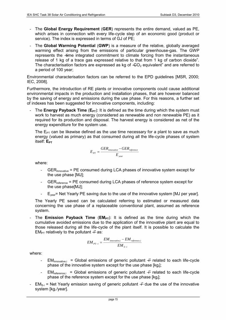
- The Energy Payback Time (EPT): It is defined as the time during which the system must work to harvest as much energy (considered as renewable and non renewable PE) as it required for its production and disposal. The harvest energy is considered as net of the energy expenditure for the system use.
The EPT can be likewise defined as the use time necessary for a plant to save as much energy (valued as primary) as that consumed during all the life-cycle phases of system itself: EPT
year
referenceinnovative
PTE
GERGERE
where:
- GERInnovative = PE consumed during LCA phases of innovative system except for the use phase [MJ];
- GERreference = PE consumed during LCA phases of reference system except for the use phase[MJ];
- Eyear= Net Yearly PE saving due to the use of the innovative system [MJ per year].
The Yearly PE saved can be calculated referring to estimated or measured data concerning the use phase of a replaceable conventional plant, assumed as reference system.
- The Emission Payback Time (EMPT): It is defined as the time during which the cumulative avoided emissions due to the application of the innovative plant are equal to those released during all the life-cycle of the plant itself. It is possible to calculate the EMPT relatively to the pollutant ―i‖ as:
iS
ireferenceiinnovative
iPTEM
EMEMEM
,,
where:
- EMinnovative,i = Global emissions of generic pollutant ―i‖ related to each life-cycle phase of the innovative system except for the use phase [kgi];
- EMreference,i = Global emissions of generic pollutant ―i‖ related to each life-cycle phase of the reference system except for the use phase [kgi];
- EMS-i = Net Yearly emission saving of generic pollutant ―i‖ due the use of the innovative system [kgi /year].
IEA SHC Task 38 Solar Air Conditioning and Refrigeration Subtask D3, December 2010
page 16
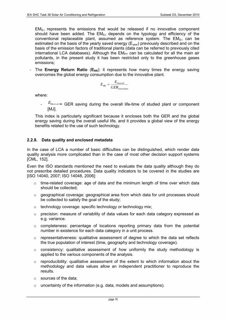
EMS-i represents the emissions that would be released if no innovative component should have been added. The EMS-i depends on the typology and efficiency of the conventional replaceable plant, assumed as reference system. The EMS-i can be estimated on the basis of the yearly saved energy (Eyear) previously described and on the basis of the emission factors of traditional plants (data can be referred to previously cited international LCA databases). Although the EMPT can be calculated for all the main air pollutants, in the present study it has been restricted only to the greenhouse gases emissions;
- The Energy Return Ratio (ERR): it represents how many times the energy saving overcomes the global energy consumption due to the innovative plant.
innovative
Overall
RRGER
EE
where:
- Over al lE = GER saving during the overall life-time of studied plant or component [MJ].
This index is particularly significant because it encloses both the GER and the global energy saving during the overall useful life, and it provides a global view of the energy benefits related to the use of such technology.
2.2.8. Data quality and enclosed metadata
In the case of LCA a number of basic difficulties can be distinguished, which render data quality analysis more complicated than in the case of most other decision support systems [CML, 152].
Even the ISO standards mentioned the need to evaluate the data quality although they do not prescribe detailed procedures. Data quality indicators to be covered in the studies are [ISO 14040, 2007; ISO 14048, 2006]:
o time-related coverage: age of data and the minimum length of time over which data should be collected;
o geographical coverage: geographical area from which data for unit processes should be collected to satisfy the goal of the study;
o technology coverage: specific technology or technology mix;
o precision: measure of variability of data values for each data category expressed as e.g. variance.
o completeness: percentage of locations reporting primary data from the potential number in existence for each data category in a unit process.
o representativeness: qualitative assessment of degree to which the data set reflects the true population of interest (time, geography and technology coverage).
o consistency: qualitative assessment of how uniformly the study methodology is applied to the various components of the analysis.
o reproducibility: qualitative assessment of the extent to which information about the methodology and data values allow an independent practitioner to reproduce the results.
o sources of the data;
o uncertainty of the information (e.g. data, models and assumptions).
IEA SHC Task 38 Solar Air Conditioning and Refrigeration Subtask D3, December 2010
page 17
Several methodologies and approaches have been suggested for the management of data quality in LCA [Heijungs, 1996; Kennedy et al. 1997; Meier, 1997; Weidema, 1996; Wrisberg, 1997]. These are often complicated and time-consuming, requiring a detailed knowledge of systems.
For these reason it has been decided to include in the data reporting sheet a set of additional data (metadata) concerning the study, the considered technical system, the data sources, the main assumptions and rules.
It is also suggest a self ―data quality‖ statement, where the analyst could consider the limits of the study, the strong and weak points, and general completeness, representativeness and reproducibility of the results.
Finally, authors should insert a text sheet where to insert further information concerning the investigated system and its peculiarities. In particular, useful information could regard the incidence of each life cycle step.
2.2.9. Data reporting framework
A data reporting framework for the presentation of data has been prepared and attached in Annex I. The report sheets aims to lead the authors into compile and report the most significant information concerning their study, and to present the LCA results in a standardized format. The sheets have been inspired to the EPD scheme, introducing new descriptive elements that reflex the previous discussed key-issues.
In the case-study report, authors should compile a brief description of their studied system, and to compile the sheets as following:
1. Product: Insert the name of the investigated product or technology;
2. Authors and reference: Insert the name of authors and the study reference;
3. Description of the product: insert a description of the main product components and functionalities, belonging technologies, and main system characteristics, in order to clarify and improve the comprehension of the next LCA steps;
4. Product characteristics: Insert some specific technical characteristics (as nominal power, useful surface, plant output). These data are useful for the calculation of the specific FUs eco-profiles. A detailed description of the working phase and efficiency should be included, in order to better evaluate the environmental impacts during the system utilization.
5. Metadata: as previously explained, metadata are the additional information that improve the understanding, the transparency and the quality of LCA studies. Furthermore metadata improve the comparability of different studies, giving information about methodological and empirical choices. Information to be included in the report are:
a. Age of the study: including the year of the study and;
b. Technological representativeness of input data: it concerns the representativeness of input LCA data employed during the inventory phase and the main assumptions on data availability;
c. System boundaries: with a description of LCA phase that have been included/excluded from the analysis and the description of possible deviations from the general assumptions previously described in paragraph 2.1.2;
d. Useful life-time: assessed or measured data of the plant‘s working time;
IEA SHC Task 38 Solar Air Conditioning and Refrigeration Subtask D3, December 2010
page 18
e. Cut-off rules: description of rules for the exclusions of components in the study, and description of the possible deviations from the general assumptions previously described in paragraph 2.1.3;
f. Allocation rules: description of the allocation processes, and description of the possible deviations from the general assumptions previously described in paragraph 2.1.4;
g. Further details: additional information that could improve the completeness of the results;
h. Quality data assessment: introducing a qualitative description of the consistency of the main employed data, their consistency and representativeness, the age of input data and their suitability for the study purposes;
6. Life Cycle inventory: including a description of the main system‘s raw materials, air and water emissions, and produced wastes;
7. Product eco-profile: a synthesis of the main environmental global indexes, as previously described in paragraph 2.1.6;
8. Primary energy saving: concerning the RE systems and the innovative components, it is possible to calculate the possible benefits and drawbacks related to the use of such technologies and additional elements. The calculation of energy and emission saving, as described into paragraph 2.1.9, requires a detailed definition and description of a reference system which compare the case-study to;
9. Payback indexes: they involve information about system impacts and benefits, trying to make a global life cycle balance and to give to regards a synthetic information about life-cycle performances of the plants.

IEA SHC Task 38 Solar Air Conditioning and Refrigeration Subtask D3, December 2010
page 19
ANNEX I : Data Report format

IEA SHC Task 38 Solar Air Conditioning and Refrigeration Subtask D3, December 2010
page 20

IEA SHC Task 38 Solar Air Conditioning and Refrigeration Subtask D3, December 2010
page 21
3. LCA Case Studies
3.1 Solar Cooling systems with Ad, Ab, VC chillers
3.1.1 Definition of case studies
Four different cases have been investigated in order to assess the performances of two
different technologies of thermally driven chillers (Absorption - Ab and Adsorption - Ad) in two
applications represented by a building loads in two localities: Palermo (South Italy) and
Zurich (Switzerland).
All the systems use two pipes fan coils for cooling and heating distribution.
In addition we have decided also to include two possible alternatives in the configurations
according to the modality of back-up of the solar cooling systems in summer operation The
first case includes an auxiliary conventional chiller supporting the ad/absorption chiller, and it
is defined as ―cold back-up‖. In the second configuration an auxiliary gas boiler, supports the
solar system and the ad/absorption chiller heat input; it is defined as ―hot-back-up‖.
The four basic systems (to be analysed in two locations) resulted to be:
- SHC with Absorption machine (12 kW) and 35 m2 evacuated tubes with hot-back-up
in summer operation
- SHC with Absorption machine (12 kW) and 35 m2 evacuated tubes with cold-back-up
in summer operation
- SHC with Adsorption machine (8 kW) and 25 m2 flat plate collectors with hot-back-up
in summer operation
- SHC with Adsorption machine (8 kW) and 25 m2 flat plate collectors with cold-back-up
in summer operation
In this way the number of investigated combinations systems/load was 8.
More details about the plants will be provided in the next chapters.
The performances of these 4 systems has been compared to a reference heating and
cooling defined by: Conventional system with a vapour compression (VC) chiller and a gas
boiler.
The first step of the analysis was to calculate, by means of TRNSYS simulations, the energy
performances of the selected SHC plants with different technologies and sizes (adsorption
machine of 8 kW – absorption machine of 12 kW), for two localities (Palermo and Zurich)
with different climatic conditions. Simulations were carried out with meteorological data from
the database METEONORM with following peak conditions.

IEA SHC Task 38 Solar Air Conditioning and Refrigeration Subtask D3, December 2010
page 22
Table 2: Meteo conditions for the two selected climates
Zurich Palermo
summer Tmax = 30.9 °C, xmax = 13.5 g/kg Tmax = 35.8 °C, xmax = 24.3 g/kg
winter Tmin = -11.5 °C xmin = 1.2 g/kg Tmin = 5.2 °C xmin = 4.6 g/kg
For this reason four different buildings have been defined in order to have a cooling peak
load of 8 kW and of 12 kW in both climatic conditions and the hourly H/C load profile for the
typical year.
The buildings have been simulated with type 56b ―Multizone Building‖ (TRNSYS version
16.1).
The following general conditions have been assumed for the simulation:
- Set point temperature for cooling: 26°C
- Set point temperature set point for heating: 20°C
- Relative humidity of set point: 50%
- Infiltration of external air: 0.6/h during the day, 0.1/h during the night
Table 3: Design data for load calculation
Zürich building Palermo building Uwall,roof 0.2 W/m2K Uwall,roof 0.48 W/m2K Uwindow 1.1 W/m2K Uwindow 1.8 W/m2K Gsolar = 0.6 Gsolar = 0.7 shading factor: 10 % winter 40 % summer shading factor: 60 %
Internal load : 6 W/m2 start cooling: end heating start cooling: end heating 15-May 14-May 15-May 30-March end cooling: start heating end cooling: start heating 14-Sept 15-Sept 30-Sept 1-Dec
All buildings have two floors, similar geometric features and the same relation wall/window
on every side.
At these conditions, the simulated load profiles came out as showed in Table4.
For every building, monthly load profiles have been created by simulation (Table5).
IEA SHC Task 38 Solar Air Conditioning and Refrigeration Subtask D3, December 2010
page 23
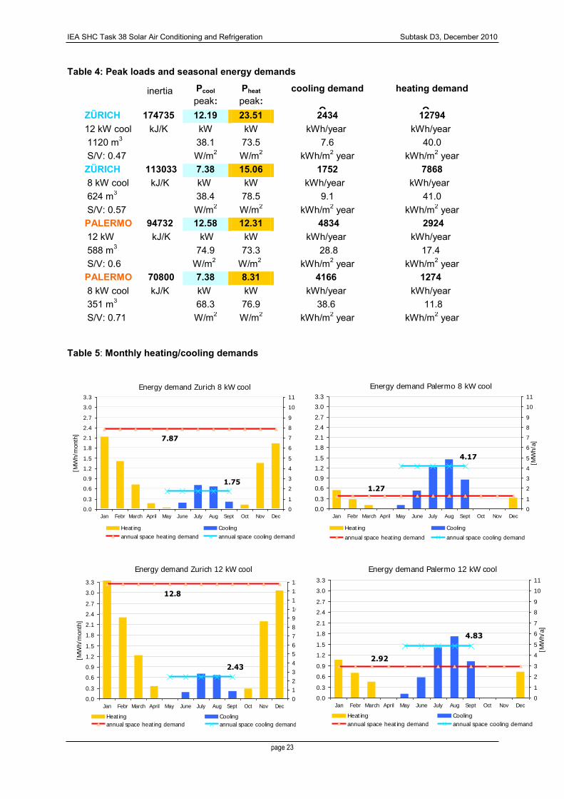
Table 4: Peak loads and seasonal energy demands
inertia Pcool
peak: Pheat
peak: cooling demand
Qcool
heating demand
Qheat ZÜRICH 174735 12.19 23.51 2434 12794 12 kW cool kJ/K kW kW kWh/year kWh/year 1120 m3 38.1 73.5 7.6 40.0 S/V: 0.47 m2/m3
W/m2 W/m2 kWh/m2 year kWh/m2 year ZÜRICH 113033 7.38 15.06 1752 7868 8 kW cool kJ/K kW kW kWh/year kWh/year 624 m3 38.4 78.5 9.1 41.0 S/V: 0.57 m2/m3
W/m2 W/m2 kWh/m2 year kWh/m2 year PALERMO 94732 12.58 12.31 4834 2924 12 kW cool
kJ/K kW kW kWh/year kWh/year 588 m3 74.9 73.3 28.8 17.4 S/V: 0.6 m2/m3
W/m2 W/m2 kWh/m2 year kWh/m2 year PALERMO 70800 7.38 8.31 4166 1274 8 kW cool kJ/K kW kW kWh/year kWh/year 351 m3 68.3 76.9 38.6 11.8 S/V: 0.71 m2/m3
W/m2 W/m2 kWh/m2 year kWh/m2 year
Table 5: Monthly heating/cooling demands
Energy demand Zurich 8 kW cool
7.87
1.75
0.0
0.3
0.6
0.9
1.2
1.5
1.8
2.1
2.4
2.7
3.0
3.3
Jan Febr March April May June July Aug Sept Oct Nov Dec
[MW
h/m
onth
]
0
1
2
3
4
5
6
7
8
9
10
11
Heating Cooling
annual space heating demand annual space cooling demand
Energy demand Palermo 8 kW cool
1.27
4.17
0.0
0.3
0.6
0.9
1.2
1.5
1.8
2.1
2.4
2.7
3.0
3.3
Jan Febr March April May June July Aug Sept Oct Nov Dec
0
1
2
3
4
5
6
7
8
9
10
11
[MW
h/a
]Heating Cooling
annual space heating demand annual space cooling demand
Energy demand Zurich 12 kW cool
12.8
2.43
0.0
0.3
0.6
0.9
1.2
1.5
1.8
2.1
2.4
2.7
3.0
3.3
Jan Febr March April May June July Aug Sept Oct Nov Dec
[MW
h/m
onth
]
0
1
2
3
4
5
6
7
8
9
10
11
12
13
Heating Cooling
annual space heating demand annual space cooling demand
Energy demand Palermo 12 kW cool
2.92
4.83
0.0
0.3
0.6
0.9
1.2
1.5
1.8
2.1
2.4
2.7
3.0
3.3
Jan Febr March April May June July Aug Sept Oct Nov Dec
0
1
2
3
4
5
6
7
8
9
10
11
[MW
h/a
]
Heating Cooling
annual space heating demand annual space cooling demand

IEA SHC Task 38 Solar Air Conditioning and Refrigeration Subtask D3, December 2010
page 24
3.1.2 Air to water vapor compression chiller and gas boiler: general description of the plant
The conventional system consists mainly of two subsystems, namely:
10 kW water VC chiller (cooling unit)
20 kW gas boiler (heating system)
A schematic diagram of this system is shown in Figure 1.
Figure 1: Schematic representation of the conventional system
In this system, the cooling effect is produced by a 10 kW water vapour compression chiller
with a COP of 2.5 during the cold season. During winter, the gas boiler is employed to
provide the required heating to the building.
The energy and environmental impacts related to the use phase of the conventional plant are
summarized in Table 6.
IEA SHC Task 38 Solar Air Conditioning and Refrigeration Subtask D3, December 2010
page 25
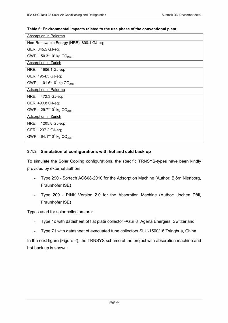
Table 6: Environmental impacts related to the use phase of the conventional plant
Absorption in Palermo
Non-Renewable Energy (NRE): 800.1 GJ-eq;
GER: 845.5 GJ-eq;
GWP: 50.3*103 kg CO2eq.
Absorption in Zurich
NRE: 1906.1 GJ-eq;
GER: 1954.3 GJ-eq;
GWP: 101.6*103 kg CO2eq.
Adsorption in Palermo
NRE: 472.3 GJ-eq;
GER: 499.8 GJ-eq;
GWP: 29.7*103 kg CO2eq.
Adsorption in Zurich
NRE: 1205.8 GJ-eq;
GER: 1237.2 GJ-eq;
GWP: 64.1*103 kg CO2eq.
3.1.3 Simulation of configurations with hot and cold back up
To simulate the Solar Cooling configurations, the specific TRNSYS-types have been kindly
provided by external authors:
- Type 290 - Sortech ACS08-2010 for the Adsorption Machine (Author: Bjòrn Nienborg,
Fraunhofer ISE)
- Type 209 - PINK Version 2.0 for the Absorption Machine (Author: Jochen Döll,
Fraunhofer ISE)
Types used for solar collectors are:
- Type 1c with datasheet of flat plate collector ―Azur 8‖ Agena Énergies, Switzerland
- Type 71 with datasheet of evacuated tube collectors SLU-1500/16 Tsinghua, China
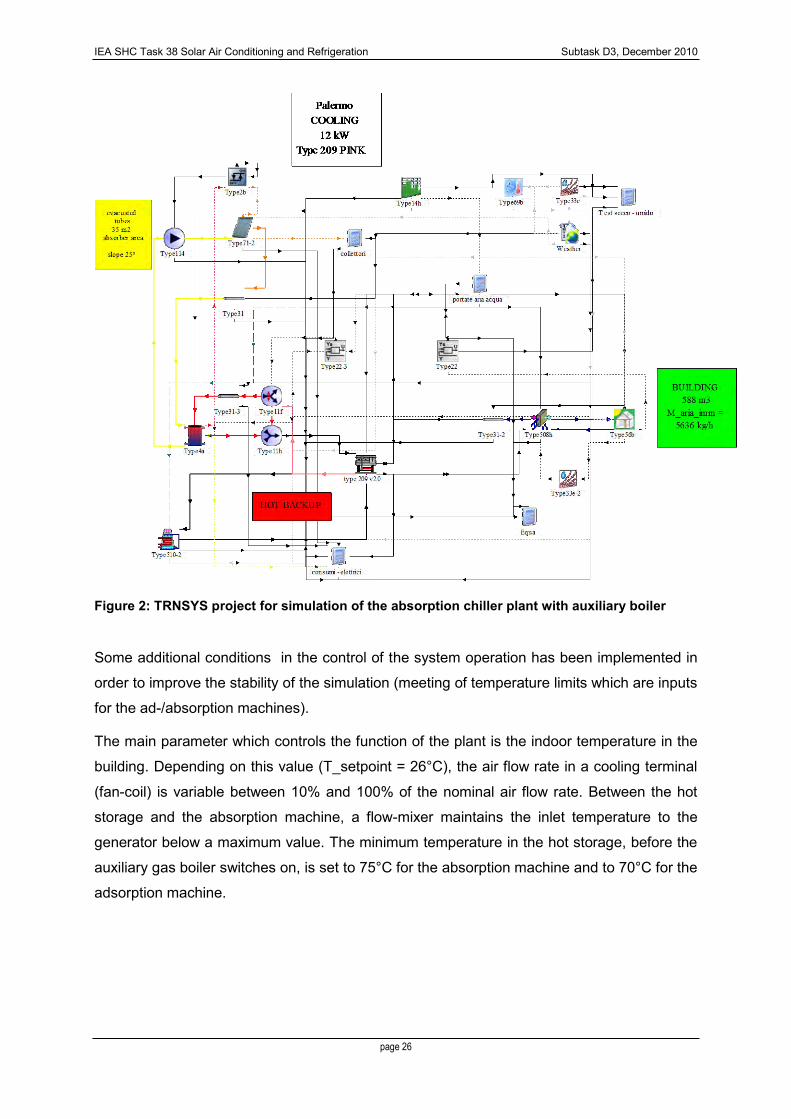
In the next figure (Figure 2), the TRNSYS scheme of the project with absorption machine and
hot back up is shown:
IEA SHC Task 38 Solar Air Conditioning and Refrigeration Subtask D3, December 2010
page 26
Figure 2: TRNSYS project for simulation of the absorption chiller plant with auxiliary boiler
Some additional conditions in the control of the system operation has been implemented in
order to improve the stability of the simulation (meeting of temperature limits which are inputs
for the ad-/absorption machines).
The main parameter which controls the function of the plant is the indoor temperature in the
building. Depending on this value (T_setpoint = 26°C), the air flow rate in a cooling terminal
(fan-coil) is variable between 10% and 100% of the nominal air flow rate. Between the hot
storage and the absorption machine, a flow-mixer maintains the inlet temperature to the
generator below a maximum value. The minimum temperature in the hot storage, before the
auxiliary gas boiler switches on, is set to 75°C for the absorption machine and to 70°C for the
adsorption machine.

IEA SHC Task 38 Solar Air Conditioning and Refrigeration Subtask D3, December 2010
page 27
Figure 3: TRNSYS project for simulation of the adsorption chiller plant with cold back up
Figure 3 represents part of TRNSYS project used for the simulation of the adsorption
configuration with cold back up. A fictive cold storage had to be inserted, in order to assure a
constant cooling load for the type of the Sortech machine, what otherwise created simulation
errors. The auxiliary chiller is connected in parallel, and switches on with a maximum outlet
temperature from the cold storage.
Heating operation has been simulated in own projects, with only solar collectors, hot storage,
auxiliary gas boiler and fan coils.
3.1.4 Simulation results
For calculation of PE consumption, following conversion have been used:
Table 7: Conversion factor for electricity and gas
SWITZERLAND ITALY
Electricity conversion factor 0.339 0.334
Gas conversion factor 0.802 0.802
In the next tables, simulation results are shown:
IEA SHC Task 38 Solar Air Conditioning and Refrigeration Subtask D3, December 2010
page 28
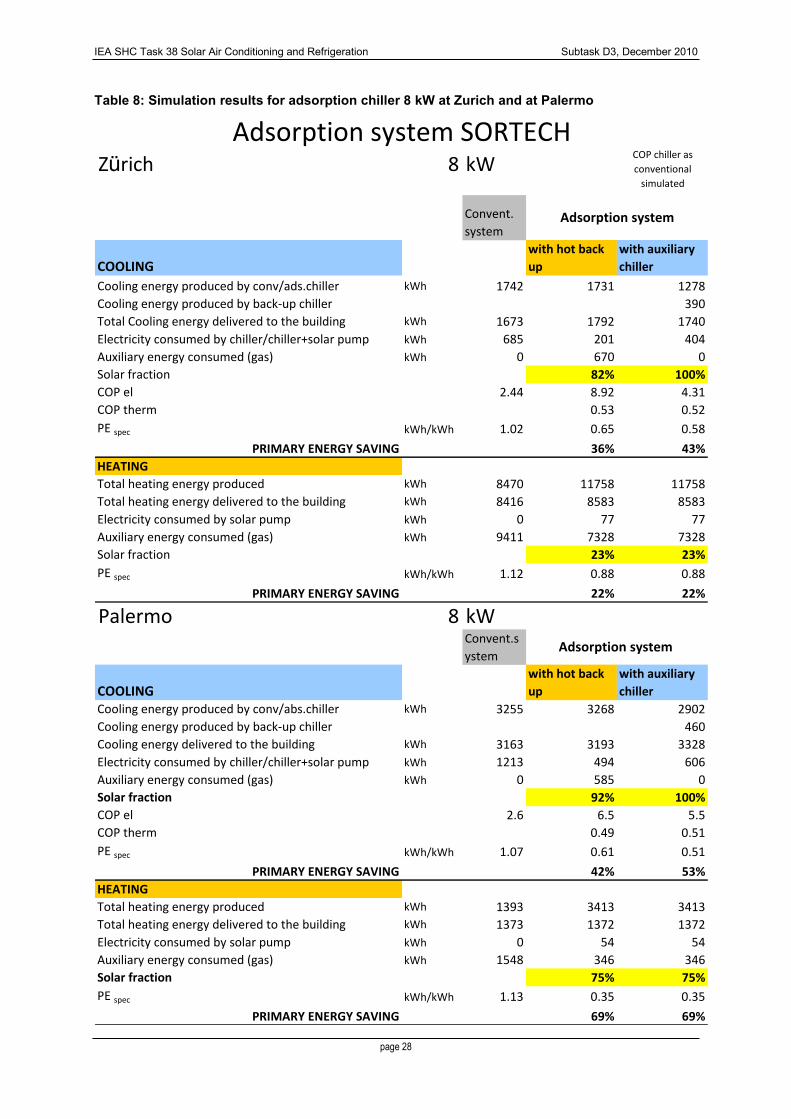
Table 8: Simulation results for adsorption chiller 8 kW at Zurich and at Palermo
Zürich 8 kW
Convent.
system
COOLINGwith hot back
up
with auxiliary
chiller
Cooling energy produced by conv/ads.chiller kWh 1742 1731 1278
Cooling energy produced by back-up chiller 390
Total Cooling energy delivered to the building kWh 1673 1792 1740
Electricity consumed by chiller/chiller+solar pump kWh 685 201 404
Auxiliary energy consumed (gas) kWh 0 670 0
Solar fraction 82% 100%
COP el 2.44 8.92 4.31
COP therm 0.53 0.52
PE spec kWh/kWh 1.02 0.65 0.58
PRIMARY ENERGY SAVING 36% 43%
HEATING
Total heating energy produced kWh 8470 11758 11758
Total heating energy delivered to the building kWh 8416 8583 8583
Electricity consumed by solar pump kWh 0 77 77
Auxiliary energy consumed (gas) kWh 9411 7328 7328
Solar fraction 23% 23%
PE spec kWh/kWh 1.12 0.88 0.88
PRIMARY ENERGY SAVING 22% 22%
Palermo 8 kW
COOLINGwith hot back
up
with auxiliary
chiller
Cooling energy produced by conv/abs.chiller kWh 3255 3268 2902
Cooling energy produced by back-up chiller 460
Cooling energy delivered to the building kWh 3163 3193 3328
Electricity consumed by chiller/chiller+solar pump kWh 1213 494 606
Auxiliary energy consumed (gas) kWh 0 585 0
Solar fraction 92% 100%
COP el 2.6 6.5 5.5
COP therm 0.49 0.51
PE spec kWh/kWh 1.07 0.61 0.51
PRIMARY ENERGY SAVING 42% 53%
HEATING
Total heating energy produced kWh 1393 3413 3413
Total heating energy delivered to the building kWh 1373 1372 1372
Electricity consumed by solar pump kWh 0 54 54
Auxiliary energy consumed (gas) kWh 1548 346 346
Solar fraction 75% 75%
PE spec kWh/kWh 1.13 0.35 0.35
PRIMARY ENERGY SAVING 69% 69%
Adsorption system
Adsorption system SORTECHCOP chiller as
conventional
simulated
Adsorption system
Convent.s
ystem

IEA SHC Task 38 Solar Air Conditioning and Refrigeration Subtask D3, December 2010
page 29
The first configuration with adsorption cooling machine 8 kW and auxiliary heater as hot back
up in Zurich reaches PE savings of only 36%, nevertheless electrical COP is extremely high
(above 8). On the other hand, the cooling energy demand is the lowest of all considered case
studies, causing poor exploitation of the machine. Using an auxiliary chiller as back-up, PE-
savings rise up to 43%.
It must be always considered that results of energy production and consumption are not-
linear, due to restrictions in the simulation of control strategies with rapid changes (for
instance electricity consumption for the external heat-exchanger).
In heating operation, PE-savings in Zurich are very low (23%), such as Solar Fraction is in
the same range.
For the Palermo climate, the configuration with hot back-up reaches 43% PE-savings, and
53% with cold back-up.
This shows that the choice of hot back-up is not convenient in case of very low thermal COP
(around 0.5 for the considered adsorption machine).
Solar Heating is, as foreseen, convenient at Palermo (Solar Fraction 75%), whereas at
Zurich a solar plant which is designed to feed a small adsorption machine, due to a higher
heating demand and lower solar radiation, provides only 23% of energy.

IEA SHC Task 38 Solar Air Conditioning and Refrigeration Subtask D3, December 2010
page 30
Table 9: Simulation results for absorption chiller 12 kW at Zurich and at Palermo
Zürich 12 kW
Convent.
system
COOLING
with hot back
up
with auxiliary
chiller
Cooling energy produced by conv/abs.chiller kWh 2438 2301 2199
Cooling energy produced by back-up chiller 182
Total Cooling energy delivered to the building kWh 2410 2325 2369
Electricity consumed by chiller/chiller+solar pump kWh 1046 655 693
Auxiliary energy consumed (gas) kWh 0 177 0
Solar fraction 94% 100%
COP el 2.30 3.55 3.42
COP therm 0.71 0.7
PE spec kWh/kWh 1.09 0.78 0.73
PRIMARY ENERGY SAVING 28% 33%
HEATING
Total heating energy produced kWh 13456 17619 17619
Total heating energy delivered to the building kWh 13380 13080 13080
Electricity consumed by solar pump kWh 0 81 81
Auxiliary energy consumed (gas) kWh 14951 10165 10165
Solar fraction 30% 30%
PE spec kWh/kWh 1.12 0.79 0.79
PRIMARY ENERGY SAVING 29% 29%
Palermo 12 kW
COOLING
with hot back
up
with auxiliary
chiller
Cooling energy produced by conv/abs.chiller kWh 4875 4659 4083
Cooling energy produced by back-up chiller 403
Cooling energy delivered to the building kWh 4899 4696 4521
Electricity consumed by chiller/chiller+solar pump kWh 1995 937 1065
Auxiliary energy consumed (gas) kWh 0 246 0
Solar fraction 96% 100%
COP el 2.5 5.0 4.2
COP therm 0.69 0.68
PE spec kWh/kWh 1.13 0.61 0.65
PRIMARY ENERGY SAVING 46% 42%
HEATING
Total heating energy produced kWh 2478 6381 6381
Total heating energy delivered to the building kWh 2455 2966 2966
Electricity consumed by solar pump kWh 0 52 52
Auxiliary energy consumed (gas) kWh 2754 414 414
Solar fraction 87% 87%
PE spec kWh/kWh 1.12 0.18 0.18
PRIMARY ENERGY SAVING 84% 84%
COP chiller as
conventional simulated
Absorption system
Absorption system PINK
Convent.
systemAbsorption system

IEA SHC Task 38 Solar Air Conditioning and Refrigeration Subtask D3, December 2010
page 31
Results reveal that the absorption chiller 12 kW at Zurich is less efficient than the first
configuration (Adsorption), with PE-savings of only 28% respectively 33% (hot/cold back-up).
This can be explained again from low cooling energy demand in the building and higher
temperature differences in the plant.
On the other hand, the larger solar collector area and use of evacuated tubes lead up to
higher Solar Fraction (30%) in heating operation.
A different scenario come out for the absorption plant 12 kW at Palermo; here the
configuration with auxiliary heater is more convenient than the one with cold back-up. In this
case the climatic conditions favor high solar heat contribution correlated with high cooling
demand. Due to good exploitation of the absorption machine, also electrical COP is relatively
high (5.0)
In heating period, likewise high PE-savings are obtained (84%).

IEA SHC Task 38 Solar Air Conditioning and Refrigeration Subtask D3, December 2010
page 32
3.1.5 Study field: FU, system boundaries, data quality, cut-off rules, assumptions
The analysis has been carried out using the LCA software SimaPro and Ecobat, the
environmental database Ecoinvent and the EPD 2007 and Cumulative Energy Demand as
impact assessment methods.
The main choices and assumptions of the LCA study are the following:
FUs:
a solar cooling plant with absorption or adsorption chiller;
1 kW of power of the main component of the plant: the absorption chiller;
1 kWh of energy produced by plant.
System boundaries: production of the main plant components, use of the plant and end-
of-life of the main plant components.
In the study have not been taken into account the energetic and environmental impacts
related to:
Transport of the plant components from the production site to the utilization site;
Transport of the plant components at the end-of-life from the utilization site to the
disposal site;
The maintenance phase.
The eco-profiles of evacuated solar thermal collectors, gas boiler, heat storage, vapor
compression chiller, pumps and piping, have been referred to Ecoinvent database: the
eco-profiles of the absorption chiller and the cooling tower have been assessed starting
from data collected in field.
The useful life of each plant component is 25 years.
The energetic and environmental impacts related to the electricity use are referred to the
Italian and Swiss energy mix.
Because of data regarding 20 kW gas boiler have not been available, they have been
estimated starting from the eco-profile of a 10 kW gas boiler and the masses of the two
gas boilers, using a conversion factor of 0.267.
Because of data about conventional vapor chiller have not been available, the eco-profile
of the chiller was estimated starting from the eco-profile of an heat-pump and using a
conversion factor of 1.53. The eco-profile of the heat-pump has been referred to
Ecoinvent database.

IEA SHC Task 38 Solar Air Conditioning and Refrigeration Subtask D3, December 2010
page 33
Data regarding the eco-profile of the pumps (with different power) have been estimated
starting from the eco-profile of a 40W pump.
Detailed metadata related to each plant component are described in Annex 2.
3.1.6 Absorption chiller
In the following, the LCA of a solar cooling plant is performed according to the LCA
standards of the ISO 14040 series [ISO 14040, 2006; ISO 14044, 2006]. The plant works
with two different configurations: hot backup and cold backup and it is installed in two
different locations: Palermo and Zurich.
3.1.6.1 General description of the plants (with cold and hot backup)
The solar absorption chiller plant, with hot backup configuration, consists mainly of five
subsystems, namely:
12 kW ammonia/water adsorption machine from Solarnext/Pink;
evacuated solar thermal collector field of 35 m2, (azimuth: south; slope: 40° at Zurich,
25° at Palermo);
2000 l hot water insulated storage tank;
35 kW wet cooling tower;
20 kW heating system (gas boiler).
A schematic diagram of this system is shown in Figure 4

IEA SHC Task 38 Solar Air Conditioning and Refrigeration Subtask D3, December 2010
page 34
Figure 4: Schematic representation of the absorption chiller plant (hot backup configuration)
The solar absorption chiller plant, with cold backup configuration, consists of the same
subsystem as above, with the cold back system which is a 10kW vapor compression chiller.
A schematic diagram of this system is shown in Figure 5.
Figure 5: Schematic representation of the absorption chiller plant (cold backup configuration)

IEA SHC Task 38 Solar Air Conditioning and Refrigeration Subtask D3, December 2010
page 35
3.1.6.2 Eco-profile of the absorption chiller
The investigated product is the SolarNext/Pink chilli®PSC12 Absorption chiller. The
absorption chiller, filled with ammonia/water solution, generates cold through a closed,
continuous cycle.
The absorption chiller consists of four main components: the generator (also named boiler or
expeller), the condenser, the evaporator and the absorber. Inside the generator (Figure 6),
hot water is supplied to the chiller through a heat exchanger. A part of the ammonia is being
expelled from the ammonia / water solution and condensed again inside the condenser. The
ammonia condensate is fed to the evaporator where it is evaporated. During this process,
heat energy is discharged from the cooling cycle which cools it down. Inside the absorber,
the ammonia is absorbed from the low concentrated refrigerant ammonia/water solution and
the cycle starts over again.
As the water chilling process produces waste heat (which is the case for compression
cooling for example), a cooling tower is required. Compared with water/lithium bromide
absorbers, ammonia absorbers differ for the pressure levels (ammonia is driven with high
pressure and water with a vacuum) and for the different evaporator temperatures.
Figure 6: Ammonia cycle into Absorption Chiller [Solarnext, 2009]
Figure 7 depicts the structure of the chiller and shows a detail of system components. Detail
of utilized masses has been analyzed in Table 10.

IEA SHC Task 38 Solar Air Conditioning and Refrigeration Subtask D3, December 2010
page 36
Pump
Plate ExchangersTube and shell
exchangers
Vessels
Framework / housing
Figure 7: The studied SolarNext/Pink Absorption Chiller
Carrying out the LCA of the investigated chiller, the following main assumptions have been
considered:
- The FU is the ―production of one complete Absorption Chiller - SolarNext/Pink
chilli®PSC12‖;
- The LCA follows a ―cradle to grave‖ approach;
- A cut off rule of 5% has been adopted. Electronic components (electric cables,
sensors, manometers and motor parts), that represent the 4.1% of the overall system
mass, have been neglected;
- System boundaries includes: production and delivery of raw materials, production
process in the factory and disposal of production wastes at the end-of-life;
- Eco-profiles of raw materials are referred to Ecoinvent database [Frischknecht et al.,
2007].
- The absorption chiller is produced in the plant of the ―Pink‖ company, sited in Austria.
Impacts related to the use of electricity refer to the Austrian energy mix. Eco-profiles
of raw materials refers to average European data;
- Concerning the assessment of the specific consumption of electricity and production
of wastes per FU, allocation has been undergone with a mass criterion. In particular,
the yearly consumption of electricity (50,000 kWh/year), the heat consumption
(155,000 kWh/year from biomass district heating) and the disposed wastes (metal
scraps 10,000 kg/year) have been allocated considering that the produced absorption
chiller represent about 4% of the yearly company‘s production;

IEA SHC Task 38 Solar Air Conditioning and Refrigeration Subtask D3, December 2010
page 37
- Concerning the insulation, Armaflex® is employed. It is a closed cell, CFC free
elastomeric rubber material made in tube and sheets form for insulating piping, ducts
and vessels. Missing data about such insulation, eco-profile of common rubber have
been considered.
The supplying of raw metal materials comes mainly from North Italy, France and North
Europe (Table 10). Few components are locally purchased. Almost all the transportations
occur by road, except a short shipping from Sweden to Denmark. Total transportations
amount to 266 tkm by large capacity trucks and 2 tkm by ship.
The production of the chiller consists mainly in the cutting, TIG welding (Tungsten Inert
Gas welding with argon gas)1 and assembling of semi-manufactured components.
Altogether, about 10 hours of TIG are carried out in the production of one boiler. A detail
of the production process flow is shown in Figure 8.
Data previously described have been implemented to describe the eco-profile of the FU.
Results are shown in Table 11, Figure 9 and Figure 10.
Table 10: Detail of system components
System Component Material Mass [kg] Supplying from:
Housing Carbon Steel 136 France
Tube&shell HEX Stainless steel 110 North Italy
Vessels Stainless steel 25 North Italy
Working solution Ammonia (60%) & water (40%) 25 Austria
Plate-HEX Stainless steel 21 Sweden
Piping Stainless steel 20 North Italy
Pumping system
Carbon Steel 15
Italy
Stainless steel 5
Aluminium 10
Copper 5
others 6
Electric, Sensors, Manometers Electronics (various) 10 Austria
Insulation Armaflex ® 4 Germany
Valves Cast iron 2 Denmark
Total 394
1 Compared to other welding technologies, TIG is characterized by lower impacts because it avoids to
use consumables electrodes. Anyway, few data have been found into references concerning TIG emissions. Some data have been derived by a private company report and it consider specific emissions of: PM10 8.16 g/hr and Mn 0.9 g/hr. Argon consumption amounts to 5.5 l/min [Krűgher, 1994].

IEA SHC Task 38 Solar Air Conditioning and Refrigeration Subtask D3, December 2010
page 38
Piping Laser-cut components
Plate exchangers
Pumping system
Switchbox
External framework
Ammoniasolution
Iron cutting and assembling
Components cutting and welding
Auxiliary components assembling
Chiller
Chiller engine
Filling
Piping Laser-cut components
Plate exchangers
Pumping system
Switchbox
External framework
Ammoniasolution
Iron cutting and assembling
Components cutting and welding
Auxiliary components assembling
Chiller
Chiller engine
Filling
Figure 8: Production diagram flow
Table 11: Energetic and environmental impacts of the absorption chiller
NRE (MJ-eq) GER (MJ-eq) GWP (kg CO2eq)
Production of chiller components 24941 23482 1399 Production process 1284 3827 68.9
Transports 700 748 44.8
End-of-life 3.0 3.2 12.6
Total 26928 28060 1525
83.68
13.64
2.670.01
Global Energy Requirement [%]
Production of chiller
components
Productive process
Transports
End-of-life
91.7
4.52.9 0.8
Global Warming Potential [%]
Production of chiller
components
Productive process
Transports
End-of-life
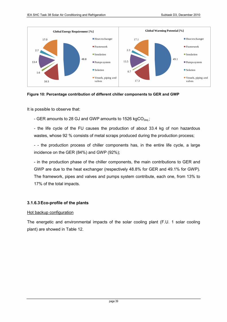
Figure 9: Percentage contribution of different phases of the chiller life-cycle to GER and GWP
IEA SHC Task 38 Solar Air Conditioning and Refrigeration Subtask D3, December 2010
page 39
48.8
16.5
1.6
13.4
2.7
17.0
Global Energy Requirement [%]
Heat exchanger
Framework
Insulation
Pumps system
Solution
Vessels, piping and
valves
49.1
17.3
0.7
13.5
2.3
17.1
Global Warming Potential [%]
Heat exchanger
Framework
Insulation
Pumps system
Solution
Vessels, piping and
valves
Figure 10: Percentage contribution of different chiller components to GER and GWP
It is possible to observe that:
- GER amounts to 28 GJ and GWP amounts to 1526 kgCO2eq.;
- the life cycle of the FU causes the production of about 33.4 kg of non hazardous
wastes, whose 92 % consists of metal scraps produced during the production process;
- - the production process of chiller components has, in the entire life cycle, a large
incidence on the GER (84%) and GWP (92%);
- in the production phase of the chiller components, the main contributions to GER and
GWP are due to the heat exchanger (respectively 48.8% for GER and 49.1% for GWP).
The framework, pipes and valves and pumps system contribute, each one, from 13% to
17% of the total impacts.
3.1.6.3 Eco-profile of the plants
Hot backup configuration
The energetic and environmental impacts of the solar cooling plant (F.U. 1 solar cooling
plant) are showed in Table 12.

IEA SHC Task 38 Solar Air Conditioning and Refrigeration Subtask D3, December 2010
page 40
Table 12: Energetic and environmental impacts of the solar cooling plant (hot backup configuration)
Components NRE (MJ-eq) GER (MJ-eq) GWP (kg CO2eq)
Production of plant
components
Absorption chiller 23457 28058 1757 Solar collectors 54987 59415 3437 Heat storage 13622 15209 852 Cooling Tower/Heat Rejection 2902 2972 154 Gas boiler 1726 1853 103 Glycol (only for plant in Zurich) 2039 2100 103 Piping+insulation 7961 8399 510 Pumps 1017 1095 66
Use phase Palermo
Cooling 258719 279604 16766 Heating 59109 60425 3556
Use phase Zurich
Cooling 166883 193422 3431 Heating 1154443 1161699 66939
End-of-life
Absorption chiller 3 3 13 Solar collectors 398 419 315 Heat storage 21 21 13 Cooling Tower/Heat Rejection 0 0 0 Gas boiler 16 17 5 Glycol (only for plant in Zurich) 459 461 39 Piping+insulation 12 13 92 Pumps 3 3 1
Total Palermo 423954 457506 27637 Total Zurich 1429949 1475160 77828
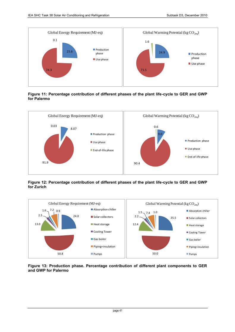
In Figure 11 and Figure 12 the contribution (%) to energy consumption and to GWP related
to each life cycle phase of the plant are showed, respectively for Palermo and Zurich. In
Figure 13 and Figure 14 the contribution (%) to energy consumption and to GWP related to
the production of the main plant components are showed, respectively for Palermo and
Zurich.
IEA SHC Task 38 Solar Air Conditioning and Refrigeration Subtask D3, December 2010
page 41
25.6
74.3
0.1
Global Energy Requirement (MJ-eq)
Production
phase
Use phase
24.9
73.5
1.6
Global Warming Potential (kg CO2eq)
Production phase
Use phase
Figure 11: Percentage contribution of different phases of the plant life-cycle to GER and GWP for Palermo
8.07
91.9
0.03
Global Energy Requirement (MJ-eq)
Production phase
Use phase
End-of-life phase
9.0
90.4
0.6
Global Warming Potential (kg CO2eq)
Production phase
Use phase
End-of-life phase
Figure 12: Percentage contribution of different phases of the plant life-cycle to GER and GWP for Zurich
24.0
50.8
13.0
2.5
1.6 7.2 0.9
Global Energy Requirement (MJ-eq)
Absorption chiller
Solar collectors
Heat storage
Cooling Tower
Gas boiler
Piping+insulation
Pumps
25.5
50.0
12.4
2.2
1.5 7.4 1.0
Global Warming Potential (kg CO2eq)
Absorption chiller
Solar collectors
Heat storage
Cooling Tower
Gas boiler
Piping+insulation
Pumps
Figure 13: Production phase. Percentage contribution of different plant components to GER and GWP for Palermo

IEA SHC Task 38 Solar Air Conditioning and Refrigeration Subtask D3, December 2010
page 42
23.6
49.9
12.8
2.5
1.61.8 7.1 0.9
Global Energy Requirement (MJ-eq)
Absorption chiller
Solar collectors
Heat storage
Cooling Tower
Gas boiler
Glycol
Piping+insulation
Pumps
25.2
49.2
12.2
2.2
1.5 1.5 7.30.9
Global Warming Potential (kg CO2eq)
Absorption chiller
Solar collectors
Heat storage
Cooling Tower
Gas boiler
Glycol
Piping+insulation
Pumps
Figure 14: Production phase. Percentage contribution of different plant components to GER and GWP for Zurich
In Table 13 and Table 14 the energetic and environmental impacts related to different F.U.s
are showed, respectively for Palermo and Zurich. To calculate the impacts related to the F.U.
―1 kWh of produced energy‖, are used the following values of produced energy in 25 years:
for Palermo 191,550 kWh, for Zurich 385,125 kWh.
Table 13: Energetic and environmental impacts of the solar cooling plant (hot backup configuration) for Palermo: comparison among different F.U.
NRE (MJ-eq) GER (MJ-eq) GWP (kg CO2eq)
F.U. 1 solar cooling plant
Production phase
105673 117000 6878 Use phase 317828 340029 20322 End-of-life phase 453 477 438
F.U. 1 kW of chiller power
Production phase
8806 9750 573 Use phase 26486 28336 1693 End-of-life phase 38 40 36
F.U. 1 kWh of produced
energy
Production phase
0.55 0.61 0.04 Use phase 1.66 1.78 0.11 End-of-life phase 0.002 0.002 0.002
Table 14: Energetic and environmental impacts of the solar cooling plant (hot backup configuration) for Zurich: comparison among different F.U.
NRE (MJ-eq) GER (MJ-eq) GWP (kg CO2eq)
F.U. 1 solar cooling plant
Production phase
107712 119101 6981 Use phase 1321326 1355121 70370 End-of-life phase 912 938 477
F.U. 1 kW of power
Production phase
8976 9925 582 Use phase 110110 112927 5864 End-of-life phase 76 78 40
F.U. 1 kWh of produced
energy
Production phase
0.28 0.31 0.02 Use phase 3.43 3.52 0.18 End-of-life phase 0.002 0.002 0.001

IEA SHC Task 38 Solar Air Conditioning and Refrigeration Subtask D3, December 2010
page 43
Cold backup configuration
The energetic and environmental impacts of the solar cooling plant (F.U.: 1 solar cooling
plant) are showed in Table 15.
Table 15: Energetic and environmental impacts of the solar cooling plant (cold backup configuration)
Components NRE (MJ-eq) GER (MJ-eq) GWP (kg CO2eq)
Production of plant
components
Absorption chiller 23457 28058 1757 Solar collectors 54987 59415 3437 Heat storage 13622 15209 852 Cooling Tower/Heat Rejection 2902 2972 154 Gas boiler 1726 1853 103 Glycol (only for plant in Zurich) 2039 2100 103 Piping+insulation 7961 8399 510 Pumps 1017 1095 66 Conventional chiller 11847 12504 2394
Use phase Palermo
Cooling 262807 286435 17223 Heating 59109 60425 3556
Use phase Zurich
Cooling 155632 183637 2403 Heating 1154443 1161699 66939
End-of-life Absorption chiller 3 3 13 Solar collectors 398 419 315 Heat storage 21 21 13
Cooling Tower/Heat Rejection 0 0 0
Gas boiler 16 17 5
Glycol (only for plant in Zurich) 459 461 39
Piping+insulation 12 13 92 Pumps 3 3 1 Conventional chiller 12 12 39
Total Palermo 439901 476854 30527 Total Zurich 1430557 1477891 79232
In Figure 15 and Figure 16 the contribution (%) to energy consumption and to GWP related
to each life cycle phase of the plant, respectively for Palermo and Zurich, are showed. In
Figure 17 and Figure 18 the contribution (%) to energy consumption and to GWP related to
the production of the main plant components, respectively for Palermo and Zurich, are
showed.

IEA SHC Task 38 Solar Air Conditioning and Refrigeration Subtask D3, December 2010
page 44
27.2
72.7
0.1
Global Energy Requirement (MJ-eq)
Production phase
Use phase
30.4
68.1
1.6
Global Warming Potential (kg CO2eq)
Production
phase
Use phase
Figure 15: Percentage contribution of different phases of the plant life-cycle to GER and GWP for Palermo
8.87
91.1
0.03
Global Energy Requirement (MJ-eq)
Production phase
Use phase
11.8
87.5
0.7
Global Warming Potential (kg CO2eq)
Production phase
Use phase
Figure 16: Percentage contribution of different phases of the plant life-cycle to GER and GWP for Zurich
21.7
45.9
11.7
2.3
1.46.5
0.89.7
Global Energy Requirement (MJ-eq)
Absorption chiller
Solar collectors
Heat storage
Cooling Tower
Gas boiler
Piping+insulation
Pumps
Conventional chiller
19.0
37.19.21.7
1.1
5.5
0.7
25.8
Global Warming Potential (kg CO2eq)
Absorption chiller
Solar collectors
Heat storage
Cooling Tower
Gas boiler
Piping+insulation
Pumps
Conventional chiller
Figure 17: Production phase. Percentage contribution of different plant components to GER and GWP for Palermo

IEA SHC Task 38 Solar Air Conditioning and Refrigeration Subtask D3, December 2010
page 45
21.3
45.1
11.6
2.3
1.4
1.6 6.40.8
9.5
Global Energy Requirement (MJ-eq)
Absorption chiller
Solar collectors
Heat storage
Cooling Tower
Gas boiler
Glycol
Piping+insulation
Pumps
Conventional chiller
18.7
36.79.1
1.6
1.1
1.1
5.4
0.7
25.5
Global Warming Potential (kg CO2eq)
Absorption chiller
Solar collectors
Heat storage
Cooling Tower
Gas boiler
Glycol
Piping+insulation
Pumps
Conventional chiller
Figure 18: Production phase. Percentage contribution of different plant components to GER and GWP for Zurich
In Table 16, Table 17 and Figure 19 the energetic and environmental impacts related to
different FUs are showed, respectively for Palermo and Zurich. To calculate the impacts
related to the FU ―1 kWh of produced energy‖, are used the following values of produced
energy in 25 years: for Palermo 187175 kWh, for Zurich 386225 kWh.
Table 16: Energetic and environmental impacts of the solar cooling plant (cold backup configuration) for Palermo: comparison among different FU.
NRE (MJ-eq) GER (MJ-eq) GWP (kg CO2eq)
F.U. 1 solar cooling plant
Production phase
117520 129505 9271 Use phase 321917 346860 20779 End-of-life phase
464 489 477
F.U. 1 kW of power
Production phase
9793 10792 773 Use phase 26826 28905 1732 End-of-life phase
39 41 40 F.U. 1 kWh of
produced energy
Production phase
0.63 0.69 0.05 Use phase 1.72 1.85 0.11 End-of-life phase
0.002 0.003 0.003
Table 17: Energetic and environmental impacts of the solar cooling plant (cold backup configuration) for Zurich: comparison among different FU.
NRE (MJ-eq) GER (MJ-eq) GWP (kg CO2eq)
FU 1 solar cooling plant
Production phase
119559 131605 9374 Use phase 1310075 1345336 69341 End-of-life phase
923 950 516
FU 1 kW of power
Production phase
9963 10967 781 Use phase 109173 112111 5778 End-of-life phase
77 79 43 FU 1 kWh of
produced energy
Production phase
0.31 0.34 0.02 Use phase 3.39 3.48 0.18 End-of-life phase
0.002 0.002 0.001

IEA SHC Task 38 Solar Air Conditioning and Refrigeration Subtask D3, December 2010
page 46
859871
1968658
859871
1968658
457506
1475160
476854
1477891
0
500000
1000000
1500000
2000000
2500000
Palermo Hot BU Zurich Hot BU Palermo Cold BU Zurich Cold BU
FU: H/C System; GER (MJ eq)
Conventional Systems
Innovative System
85987
196866
85987
196866
38125
122930
39738
123158
0
50000
100000
150000
200000
250000
Palermo Hot BU Zurich Hot BU Palermo Cold BU Zurich Cold BU
FU: 1 KW; GER (MJ)
Conventional
Systems
Innovative Systems
4,684,99
4,684,99
2,39
3,83
2,55
3,83
0,00
1,00
2,00
3,00
4,00
5,00
6,00
Palermo Hot BU Zurich Hot BU Palermo Cold BU Zurich Cold BU
FU: 1 KWh; GER
Conventional
Systems
Innovative
Systems
52863
104209
52863
104209
27637
77828
30527
79232
0
20000
40000
60000
80000
100000
120000
Palermo Hot BU Zurich Hot BU Palermo Cold BU Zurich Cold BU
FU: H/C Systems; GWP (kg CO2 eq)
Conventional Systems
Innovative System
5286
10421
5286
10421
2303
6486
2544
6603
0
2000
4000
6000
8000
10000
12000
Palermo Hot BU Zurich Hot BU Palermo Cold BU Zurich Cold BU
FU: 1 KW; GWP (kg CO2 eq)
Conventional Systems
Innovative Systems
0,290,26
0,290,26
0,14
0,20
0,16
0,21
0,00
0,05
0,10
0,15
0,20
0,25
0,30
0,35
Palermo Hot BU Zurich Hot BU Palermo Cold BU Zurich Cold BU
FU: 1 KWh; GWP (kg CO2 eq)
Conventional
Systems
Innovative Systems
Figure 19: GER and GWP Absorption Solar Cooling systems with hot and cold back-up for different FUs and in comparison with conventional heating and cooling plants
3.1.6.4 Discussion of the results for systems with absorption chiller
Regarding hot and cold backup configurations for Palermo, GER varies from 457.5 GJ to
476.8 GJ, with an increase of about 4.2%, due to an additional use of electricity in the last
configuration. GWP varies from 27637 kg CO2eq to 30527 kg CO2eq, with an increase of about
10.5%, due to the higher electricity consumption in the cold backup configuration compared
to hot backup configuration and to the use of a conventional chiller in the last configuration.
Dealing with the results for Zurich, it can be observed that GER varies from 1475.1 GJ (hot
backup configuration) to 1477.9 GJ (cold backup configuration), with an increase of about
0.18%; GWP varies from 77828 kg CO2eq (hot backup configuration) to 79232 kg CO2eq (cold
backup configuration) with an increase of about 1.8%. These increases are due to the use of
a conventional chiller in the last configuration.
Analyzing the percentage contribution of different phase of the plant life-cycle for hot and
cold backup configurations, it can be noted that the main contribution to GER and GWP is
due to the use phase. In detail, in the hot backup configuration the contribution of this phase
to GER varies from 74.3% (for Palermo) to 91.9% (for Zurich) and the contribution to GWP
varies from 73.5% (for Palermo) to 90.4% (for Zurich). In the cold backup configuration, for
IEA SHC Task 38 Solar Air Conditioning and Refrigeration Subtask D3, December 2010
page 47
Palermo the contributions of use phase to GER and GWP are, respectively, 72.7% and
68.1%; for Zurich are, respectively, 91.1% and 87.5%.
In the hot backup configuration, the production phase contributes to GER of about 25.6% for
Palermo and of about 8.1% for Zurich; the contribution to GWP is of about 25% for Palermo
and 9% for Zurich.
In the cold backup configuration, the incidence of the production phase to GER varies from
27.2% for Palermo to 8.9% for Zurich; the incidence to GWP varies from 30.4% for Palermo
to 11.8% for Zurich.
A negligible contribution to GER and GWP is related to the end-of-life phase for both
configuration and cities.
In the production phase, the main contributions to GER and GWP are due to the production
of solar collectors (45–50% for GER and 37–50% for GWP) and absorption chiller (21–24%
for GER and 19–25% for GWP).
On the basis of the results of LCA of the systems also the payback indexes (EPT, EMPT and
ERR) have been calculated.
The following table shows the figures of the three indexes for the systems using an
Absorption machine.
Table 18: Payback indexes for the case studies
E-PT EM-PT ERR year year
Palermo Hot BU 5,10 3,98 4,30
Palermo Cold BU 5,80 6,02 3,84
Zurich Hot BU 4,41 3,93 4,99
Zurich Cold BU 4,85 5,58 4,59
The indexes have been calculated taking into account the GER of the innovative system
related to the construction and end of life.
If on the other hand we decide to include the use-phase energy consumption in the GER
values all the indexes will assume negative values due to the high difference among the
energy consumption of conventional systems and the innovative one.

IEA SHC Task 38 Solar Air Conditioning and Refrigeration Subtask D3, December 2010
page 48
0.00
1.00
2.00
3.00
4.00
5.00
6.00
Palermo Hot BUPalermo Cold BU
Zurich Hot BU
Zurich Cold BU
5.10
5.80
4.414.85
Energy Payback Time (years)
Ept
Figure 20:EPT for Absorption Solar Cooling systems with hot and cold back-up
The EPT (Figure 20) is for the case studies Zurich lower than in Palermo. The main reason is
the highest use of the system all year round due to the very low heating energy demand in
winter in Palermo.
Best results are achieved in general with the configuration with hot back up. This is due to
the fact that the systems with cold back up have an additional component (vapour
compression chiller) with respect to the ones with hot back-up.
In order to appreciate the influence of some performance parameters of the systems a
sensitivity analysis has been developed.
The parameters which have been varied from the design conditions are:
equivalent hours of cooling operation (defined as the ratio between the cooling energy
delivered and the nominal cooling power)
equivalent hours of heating operation (defined as the ratio between the heating
energy delivered and the nominal heating power)
annual consumption of electricity for cooling (with the same amount of cooling energy
delivered)
annual consumption of gas for heating (with the same amount of heating energy
delivered).

IEA SHC Task 38 Solar Air Conditioning and Refrigeration Subtask D3, December 2010
page 49
The results are shown in the following graphs. X-values represent the ratio between the
value of the parameter and its design value.
Figure 21: Relationship between EPT and several parameters for Absorption Solar Cooling systems with hot and cold back-up
This graph allows to compare the influence of the four parameters in the different case
studies.
It can be noted that the strongest slopes are the ones related to the gas consumption and
heating equivalent hours in Zurich installations. A reduction of heating equivalent hours for
heating in Zurich for the system with Hot Back Up higher than 30% can lead to EPT higher
than in Palermo. For systems with Cold Back Up this reduction must be higher than 40%.
This can be observed in the following graph.

IEA SHC Task 38 Solar Air Conditioning and Refrigeration Subtask D3, December 2010
page 50
Figure 22: Relationship between EPT and the number of equivalent hour of heating operation for Absorption Solar Cooling systems with hot and cold back-up
Figure 23: Relationship between EPT and the number of equivalent hour of cooling operation for Absorption Solar Cooling systems with hot and cold back-up
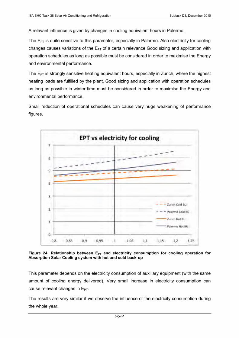
IEA SHC Task 38 Solar Air Conditioning and Refrigeration Subtask D3, December 2010
page 51
A relevant influence is given by changes in cooling equivalent hours in Palermo.
The EPT is quite sensitive to this parameter, especially in Palermo. Also electricity for cooling
changes causes variations of the EPT of a certain relevance Good sizing and application with
operation schedules as long as possible must be considered in order to maximise the Energy
and environmental performance.
The EPT is strongly sensitive heating equivalent hours, especially in Zurich, where the highest
heating loads are fulfilled by the plant. Good sizing and application with operation schedules
as long as possible in winter time must be considered in order to maximise the Energy and
environmental performance.
Small reduction of operational schedules can cause very huge weakening of performance
figures.
Figure 24: Relationship between EPT and electricity consumption for cooling operation for Absorption Solar Cooling system with hot and cold back-up
This parameter depends on the electricity consumption of auxiliary equipment (with the same
amount of cooling energy delivered). Very small increase in electricity consumption can
cause relevant changes in EPT.
The results are very similar if we observe the influence of the electricity consumption during
the whole year.

IEA SHC Task 38 Solar Air Conditioning and Refrigeration Subtask D3, December 2010
page 52
Figure 25: Relationship between EPT and gas consumption for Absorption Solar Cooling systems with hot and cold back-up
Also in this case the highest influence of this parameter is observed for the installation in
Zurich where the higher heating load is fulfilled. I must be noted that variation of about 10%
of this parameter can change the payback time of about one year.
The influence of gas consumption for heating in Palermo is almost null in this range. Very
interesting results have been obtained also for the Emissions Payback Time and ERR.
In both installations, Palermo and Zurich the time to recover the emission related to the
installation and disposal of the plant are less than six years.
ERR gives how many times the energy saving achieved overcomes the global energy
consumption of the plant life cycle. In all the cases the results are satisfactory while the
systems give back from four to five time the energy expenditure for their construction and
disposal.

IEA SHC Task 38 Solar Air Conditioning and Refrigeration Subtask D3, December 2010
page 53
0.00
1.00
2.00
3.00
4.00
5.00
6.00
7.00
Palermo Hot BUPalermo Cold
BU Zurich Hot BUZurich Cold BU
3.98
6.02
3.93
5.58
Emissions Payback Time (years)
EMpt
Figure 26: Emissions Payback Time for Absorption Solar Cooling systems with hot and cold back-up
0.00
0.50
1.00
1.50
2.00
2.50
3.00
3.50
4.00
4.50
5.00
Palermo Hot BUPalermo Cold BU
Zurich Hot BU
Zurich Cold BU
4.30
3.84
4.99
4.59
Energy Return Ratio
ER
Figure 27: ERR for Absorption Solar Cooling systems with hot and cold back-up
3.1.7 Adsorption chiller
3.1.7.1 General description of the plants (with cold and hot backup)
The solar adsorption chiller plant consists mainly of six subsystems, namely:

IEA SHC Task 38 Solar Air Conditioning and Refrigeration Subtask D3, December 2010
page 54
8 kW compact silica gel/water adsorption machine from SorTech AG (ACS 08)
flat plate collector field of 25 m2 or evacuate tubes
1300 l hot water insulated storage tank
24 kW air cooled heat exchanger (dry cooler)
20 kW heating system (gas boiler and for hot back-up configuration)
20 kW compressor chiller (for cold back-up configuration only)
A schematic diagram of this system is shown in . Figure 28.
Figure 28: Schematic representation of the adsorption chiller plant
In this system, the adsorption machine is driven by the hot water in the tank that is heated by
the solar collectors. Heat coming from the cooling circuit of the adsorption machine is
rejected by means of an air cooled heat exchanger, also known as dry cooler.
In case of insufficient solar energy, two solutions of backup system are used : (1) a gas boiler
used to heat the storage tank or (2) a chiller water unit for cooling .
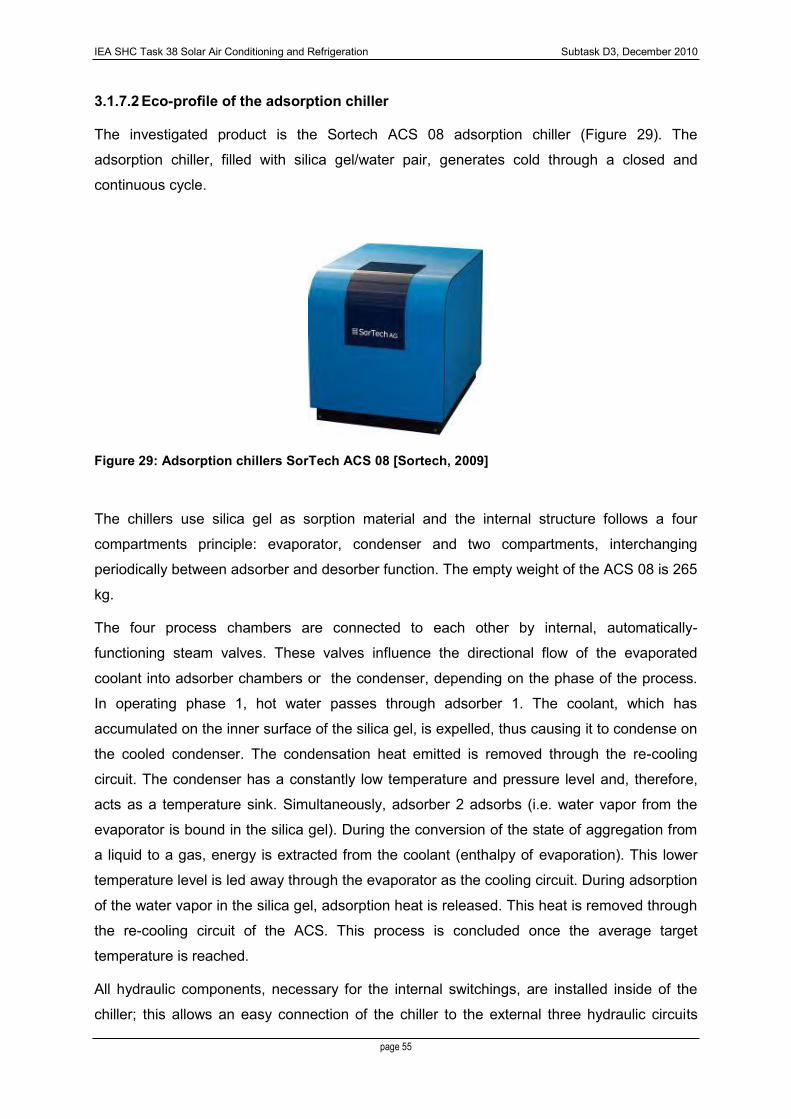
IEA SHC Task 38 Solar Air Conditioning and Refrigeration Subtask D3, December 2010
page 55
3.1.7.2 Eco-profile of the adsorption chiller
The investigated product is the Sortech ACS 08 adsorption chiller (Figure 29). The
adsorption chiller, filled with silica gel/water pair, generates cold through a closed and
continuous cycle.
Figure 29: Adsorption chillers SorTech ACS 08 [Sortech, 2009]
The chillers use silica gel as sorption material and the internal structure follows a four
compartments principle: evaporator, condenser and two compartments, interchanging
periodically between adsorber and desorber function. The empty weight of the ACS 08 is 265
kg.
The four process chambers are connected to each other by internal, automatically-
functioning steam valves. These valves influence the directional flow of the evaporated
coolant into adsorber chambers or the condenser, depending on the phase of the process.
In operating phase 1, hot water passes through adsorber 1. The coolant, which has
accumulated on the inner surface of the silica gel, is expelled, thus causing it to condense on
the cooled condenser. The condensation heat emitted is removed through the re-cooling
circuit. The condenser has a constantly low temperature and pressure level and, therefore,
acts as a temperature sink. Simultaneously, adsorber 2 adsorbs (i.e. water vapor from the
evaporator is bound in the silica gel). During the conversion of the state of aggregation from
a liquid to a gas, energy is extracted from the coolant (enthalpy of evaporation). This lower
temperature level is led away through the evaporator as the cooling circuit. During adsorption
of the water vapor in the silica gel, adsorption heat is released. This heat is removed through
the re-cooling circuit of the ACS. This process is concluded once the average target
temperature is reached.
All hydraulic components, necessary for the internal switchings, are installed inside of the
chiller; this allows an easy connection of the chiller to the external three hydraulic circuits

IEA SHC Task 38 Solar Air Conditioning and Refrigeration Subtask D3, December 2010
page 56
(high temperature source HT, heat rejection circuit MT and chilled water circuit LT). The
basic hydraulic structure of the chillers is presented in Figure 30. [Rupp et al., 2009] and
[Sortech 2009].
Figure 30: Main internal hydraulic components of the SorTech chiller and external connections. The figure presents the operation phase, of which the upper of the two sorption compartments is currently being desorbed by applying hot water and the lower sorption compartment is working as adsorber, thus taking up the vaporized refrigerant. The refrigerant circle, either fluid or vaporized, is not included into the figure. [Rupp, 2009]
The LCIA of the adsorption chiller has been done, thanks to the information given by
Sortech. The following assumptions have been taken, regarding the calculation of
one adsorption chiller ACS08:
All materials have been taken in account excluded some vacuum components
representing less than 1% of the mass.
The energy use for the fabrication of the chiller has not been taken in account.
The transport of the materials to the plant is not taken in account, because we
do not have those information.
At the end, the impacts related to the chiller include the materials use for the
fabrication and their end-of-life. The Table 19 gives the total impacts for the three
indicators for the Sortech chiller. Those impacts are not detailed by materials, as the
company want to keep this information rather confidential. Therefore, hereafter it will
consider as a black box.

IEA SHC Task 38 Solar Air Conditioning and Refrigeration Subtask D3, December 2010
page 57
Table 19: Environmental impacts of one Sortech adsorption chiller (265kg empty)
NRE (MJ-eq) GER (MJ-eq) GWP (kg CO2-eq)
Production of chiller components 22‘202 24‘187 1‘380
End-of-life 12 12 21
Total 22‘214 24‘199 1‘401
The contribution of the production is close to 100% for the NRE and GER and close to 98.5%
for the GWP. The impacts of the elimination phase are very low, as most of the components
use in the chiller can be recycled. The small impacts are related to some plastics and electric
components that cannot be recycled.
The impacts of the energy phase for the production and the transport phase would not give
much more on the total impacts on the whole installation.
3.1.7.3 Eco-profile of the plants
Configuration A) Hot backup
The environmental impacts of the adsorption solar chiller (F.U. 1 solar chiller) are showed in
Table 20. The glycol use in the plant for the Zurich location is needed in winter. No glycol is
used at Palermo location. The results are presented for three different phases: production
phase of the plant components, use phase and end-of-life phase of the components.
In Figure 31:Production phase: Percentage contribution of different plant components to
GER and GWP for Palermo and Figure 32: Production phase: Percentage contribution of
different plant components to GER and GWP for Zurich the contributions (expressed in %) of
the global PE consumption and of the GWP related to the production of the main plant
components are showed, respectively for Palermo and Zurich. For both climates, the solar
collectors are the most impacting followed by the production of the adsorption chiller. Gas
boiler as Piping+insulation and glycol are negligible but not insignificant (1.0% and more).
The difference between both climates is the glycol containing in the Zurich system.
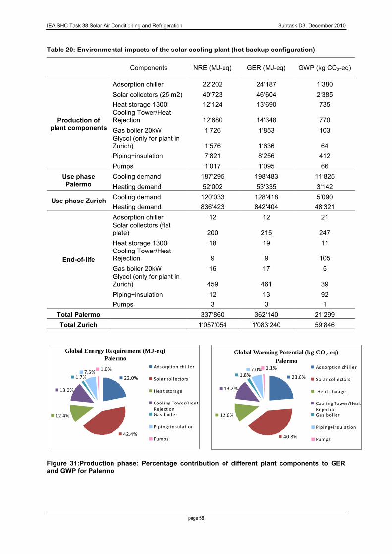
IEA SHC Task 38 Solar Air Conditioning and Refrigeration Subtask D3, December 2010
page 58
Table 20: Environmental impacts of the solar cooling plant (hot backup configuration)
Components NRE (MJ-eq) GER (MJ-eq) GWP (kg CO2-eq)
Production of plant components
Adsorption chiller 22‘202 24‘187 1‘380 Solar collectors (25 m2) 40‘723 46‘604 2‘385 Heat storage 1300l 12‘124 13‘690 735 Cooling Tower/Heat Rejection 12‘680 14‘348 770 Gas boiler 20kW 1‘726 1‘853 103 Glycol (only for plant in Zurich) 1‘576 1‘636 64 Piping+insulation 7‘821 8‘256 412 Pumps 1‘017 1‘095 66
Use phase Palermo
Cooling demand 187‘295 198‘483 11‘825 Heating demand 52‘002 53‘335 3‘142
Use phase Zurich Cooling demand 120‘033 128‘418 5‘090 Heating demand 836‘423 842‘404 48‘321
End-of-life
Adsorption chiller 12 12 21 Solar collectors (flat plate) 200 215 247 Heat storage 1300l 18 19 11 Cooling Tower/Heat Rejection 9 9 105 Gas boiler 20kW 16 17 5 Glycol (only for plant in Zurich) 459 461 39 Piping+insulation 12 13 92 Pumps 3 3 1
Total Palermo 337‘860 362‘140 21‘299 Total Zurich 1‘057‘054 1'083‘240 59‘846
Global Energy Requirement (MJ-eq)
Palermo
22.0%7.5%
12.4%
42.4%
13.0%
1.7%
1.0% Adsorption chi l ler
Solar col lectors
Heat s torage
Cool ing Tower/HeatRejectionGas boi ler
Piping+insulation
Pumps
Global Warming Potential (kg CO2-eq)
Palermo
23.6%
12.6%
7.0% 1.1%
1.8%
13.2%
40.8%
Adsorption chi l ler
Solar col lectors
Heat s torage
Cool ing Tower/HeatRejectionGas boi ler
Piping+insulation
Pumps
Figure 31:Production phase: Percentage contribution of different plant components to GER and GWP for Palermo

IEA SHC Task 38 Solar Air Conditioning and Refrigeration Subtask D3, December 2010
page 59
Global Energy Requirement (MJ-eq)
Zurich
21.7%
41.7%
12.3%
1.0%1.5%
1.7%
12.8%
7.4%Adsorption chi l ler
Solar col lectors
Heat s torage
Cool ing Tower/Heat
RejectionGas boi ler
Glycol
Piping+insulation
Pumps
Global Warming Potential (kg CO2-eq)
Zurich
23.3%
40.3%
1.1%1.1%1.7%
13.0%
12.4%
7.0% Adsorption chi l ler
Solar col lectors
Heat s torage
Cool ing Tower/Heat
RejectionGas boi ler
Glycol
Piping+insulation
Pumps
Figure 32: Production phase: Percentage contribution of different plant components to GER and GWP for Zurich
The Figure 33: Relative contribution of the three different phases for the whole life-cycle to
GER and GWP for Palermo and Figure 34: Relative contribution of the three different phases
for the whole life-cycle to GER and GWP for Zurich show the contributions (expressed in %)
of the global PE consumption and of the GWP related to each life cycle phase of the plant,
respectively for Palermo and Zurich. The most impacting phase is the use phase in both
climates. The production phase represents more impacts in Palermo then in Zurich, due to
the great demand in heating for winter. The end-of-life is negligible, even with the glycol part
in Zurich.
In Table 21 and Table 22 the environmental impacts related to different F.U.s are showed,
respectively for Palermo and Zurich. To calculate the impacts related to the F.U. ―1 KW of the
adsorption chiller power‖, an 8kW power is used and to the. F.U. ―1 kWh of produced
energy‖, the following values of produced energy in 25 years are used: for Palermo 114‘125
kWh, for Zurich 259‘375 kWh.
Global Energy Requirement (MJ-eq)
Palermo
30.4%
69.5%
0.1%
Production phase
Use phase
End-of-l i fe phase
Global Warming Potential (kg CO2-eq)
Palermo
27.5%
70.3%
2.3%
Production phase
Use phase
End-of-l i fe phase
Figure 33: Relative contribution of the three different phases for the whole life-cycle to GER and GWP for Palermo
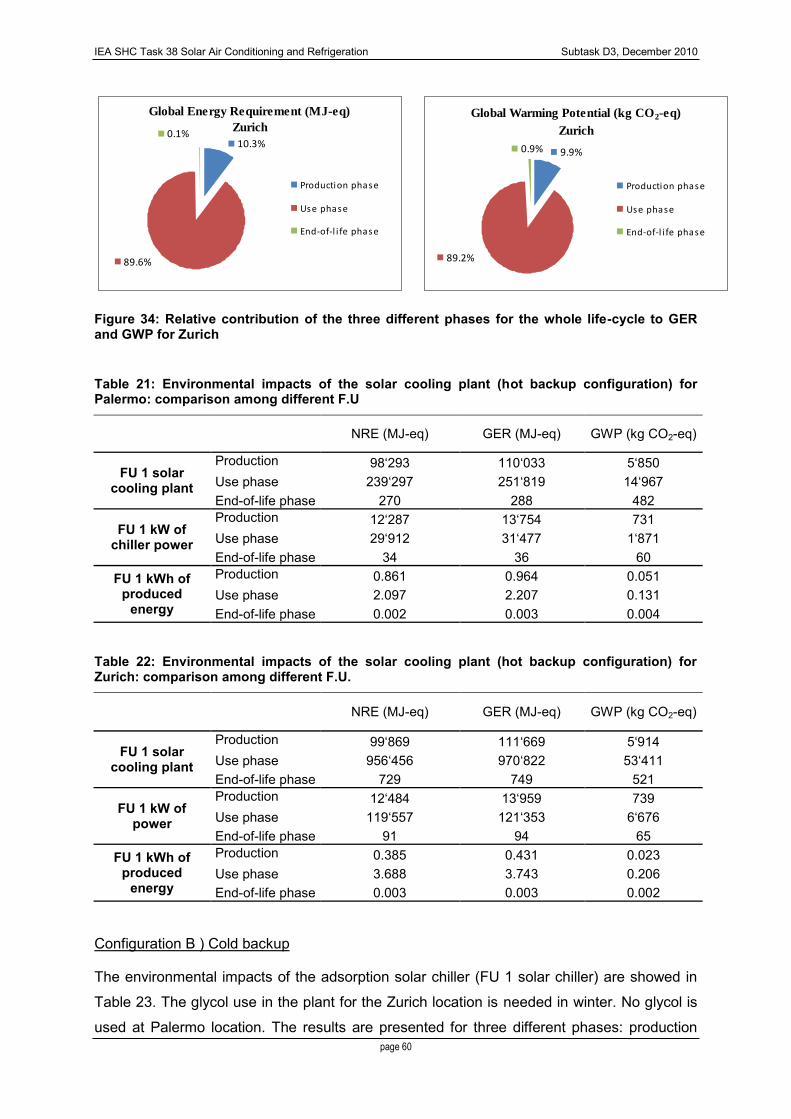
IEA SHC Task 38 Solar Air Conditioning and Refrigeration Subtask D3, December 2010
page 60
Global Energy Requirement (MJ-eq)
Zurich
10.3%
89.6%
0.1%
Production phase
Use phase
End-of-l i fe phase
Global Warming Potential (kg CO2-eq)
Zurich
9.9%0.9%
89.2%
Production phase
Use phase
End-of-l i fe phase
Figure 34: Relative contribution of the three different phases for the whole life-cycle to GER and GWP for Zurich
Table 21: Environmental impacts of the solar cooling plant (hot backup configuration) for Palermo: comparison among different F.U
NRE (MJ-eq) GER (MJ-eq) GWP (kg CO2-eq)
FU 1 solar cooling plant
Production phase
98‘293 110‘033 5‘850 Use phase 239‘297 251‘819 14‘967 End-of-life phase 270 288 482
FU 1 kW of chiller power
Production phase
12‘287 13‘754 731 Use phase 29‘912 31‘477 1‘871 End-of-life phase 34 36 60
FU 1 kWh of produced
energy
Production phase
0.861 0.964 0.051 Use phase 2.097 2.207 0.131 End-of-life phase 0.002 0.003 0.004
Table 22: Environmental impacts of the solar cooling plant (hot backup configuration) for Zurich: comparison among different F.U.
NRE (MJ-eq) GER (MJ-eq) GWP (kg CO2-eq)
FU 1 solar cooling plant
Production phase
99‘869 111‘669 5‘914 Use phase 956‘456 970‘822 53‘411 End-of-life phase 729 749 521
FU 1 kW of power
Production phase
12‘484 13‘959 739 Use phase 119‘557 121‘353 6‘676 End-of-life phase 91 94 65
FU 1 kWh of produced
energy
Production phase
0.385 0.431 0.023 Use phase 3.688 3.743 0.206 End-of-life phase 0.003 0.003 0.002
Configuration B ) Cold backup
The environmental impacts of the adsorption solar chiller (FU 1 solar chiller) are showed in
Table 23. The glycol use in the plant for the Zurich location is needed in winter. No glycol is
used at Palermo location. The results are presented for three different phases: production

IEA SHC Task 38 Solar Air Conditioning and Refrigeration Subtask D3, December 2010
page 61
phase of the plant components, use phase and end-of-life phase of the components. The
conventional chiller is adding for the cooling backup.
The Figure 35: Production phase: Percentage contribution of different plant components to
GER and GWP for Palermo and 36 show the contributions (expressed in %) of the global PE
consumption and of the GWP related to the production of the main plant components,
respectively for Palermo and Zurich, are showed. The adding of the conventional chiller is
not negligible. It represents more than 10% of the GER impacts and around 29% of the
GWP. For this last indicator, it represents as much impacts as the solar collectors see before
as the higher impacts in both indicators. The rest of the components have the same
proportion of impact as for the hot backup.
Table 23: Environmental impacts of the solar cooling plant (cold backup configuration)
Components NRE (MJ-eq) GER (MJ-eq) GWP (kg CO2-eq)
Production of plant
components
Adsorption chiller 22‘202 24‘187 1‘380 Solar collectors 25m2 40‘723 46‘604 2‘385 Heat storage 1300l 12‘124 13‘690 735 Cooling Tower/Heat Rejection 12‘680 14‘348 770 Gas boiler 1‘726 1‘853 103 Glycol (only for plant in Zurich) 1‘576 1‘636 64 Piping+insulation 7‘821 8‘256 412 Pumps 1‘017 1‘095 66 Conventional chiller 11‘847 12‘504 2‘394
Use phase Palermo
Cooling demand 149‘541 162‘985 9‘800 Heating demand 52‘002 53‘335 3‘142
Use phase Zurich
Cooling demand 90‘729 107‘055 1‘401 Heating demande 836‘423 842‘404 48‘321
End-of-life Adsorption chiller 12 12 21 Solar collectors (25m2) 200 215 247 Heat storage 1300l 18 19 11
Cooling Tower/Heat Rejection 9 9 105
Gas boiler 16 17 5
Glycol (only for plant in Zurich) 459 461 39
Piping+insulation 12 13 92 Pumps 3 3 1 Conventional chiller 12 12 39
Total Palermo 311‘965 339‘158 21‘708 Total Zurich 1‘039‘608 1'074‘394 58‘590
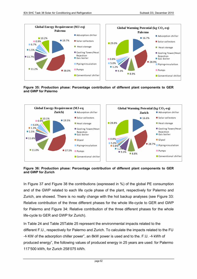
IEA SHC Task 38 Solar Air Conditioning and Refrigeration Subtask D3, December 2010
page 62
Global Energy Requirement (MJ-eq)
Palermo
19.7%
38.0%11.2%
6.7%0.9%
10.2%
11.7%
1.5%
Adsorption chi l ler
Solar col lectors
Heat s torage
Cool ing Tower/HeatRejectionGas boi ler
Piping+insulation
Pumps
Conventional chi l ler
Global Warming Potential (kg CO2-eq)
Palermo
16.7%
28.9%
8.9%
29.0%
5.0%
0.8%
1.2%
9.3%
Adsorption chi l ler
Solar col lectors
Heat s torage
Cool ing Tower/Heat
RejectionGas boi ler
Piping+insulation
Pumps
Conventional chi l ler
Figure 35: Production phase: Percentage contribution of different plant components to GER and GWP for Palermo
Global Energy Requirement (MJ-eq
Zurich)
19.5%
37.5%11.0%
6.6%
0.9%10.1%
1.3%
1.5%
11.6%
Adsorption chi l ler
Solar col lectors
Heat s torage
Cool ing Tower/HeatRejectionGas boi ler
Glycol
Piping+insulation
Pumps
Conventional chi l ler
Global Warming Potential (kg CO2-eq)
Zurich
16.6%
28.8%
5.0%
0.8%
28.7%0.8%
1.2%9.3%
8.8%
Adsorption chi l ler
Solar col lectors
Heat s torage
Cool ing Tower/HeatRejectionGas boi ler
Glycol
Piping+insulation
Pumps
Conventional chi l ler
Figure 36: Production phase: Percentage contribution of different plant components to GER and GWP for Zurich
In Figure 37 and Figure 38 the contributions (expressed in %) of the global PE consumption
and of the GWP related to each life cycle phase of the plant, respectively for Palermo and
Zurich, are showed. There is no really change with the hot backup analyses (see Figure 33:
Relative contribution of the three different phases for the whole life-cycle to GER and GWP
for Palermo and Figure 34: Relative contribution of the three different phases for the whole
life-cycle to GER and GWP for Zurich).
In Table 24 and Table 25Table 25 represent the environmental impacts related to the
different F.U., respectively for Palermo and Zurich. To calculate the impacts related to the FU
―1 KW of the adsorption chiller power‖, an 8kW power is used and to the. F.U. ―1 kWh of
produced energy‖, the following values of produced energy in 25 years are used: for Palermo
117‘500 kWh, for Zurich 258‘075 kWh.
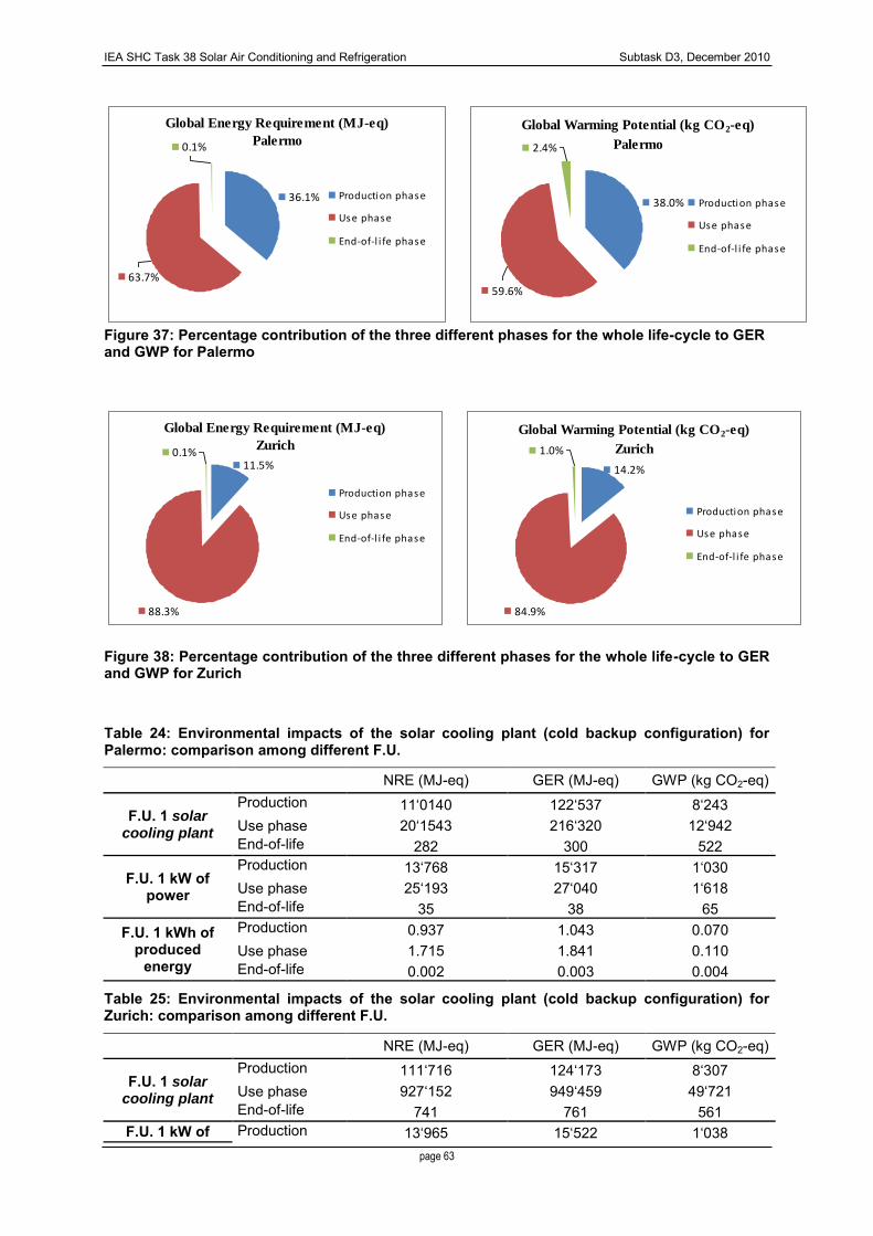
IEA SHC Task 38 Solar Air Conditioning and Refrigeration Subtask D3, December 2010
page 63
Global Energy Requirement (MJ-eq)
Palermo
36.1%
63.7%
0.1%
Production phase
Use phase
End-of-l i fe phase
Global Warming Potential (kg CO2-eq)
Palermo
38.0%
59.6%
2.4%
Production phase
Use phase
End-of-l i fe phase
Figure 37: Percentage contribution of the three different phases for the whole life-cycle to GER and GWP for Palermo
Global Energy Requirement (MJ-eq)
Zurich
88.3%
0.1%11.5%
Production phase
Use phase
End-of-l i fe phase
Global Warming Potential (kg CO2-eq)
Zurich
84.9%
14.2%
1.0%
Production phase
Use phase
End-of-l i fe phase
Figure 38: Percentage contribution of the three different phases for the whole life-cycle to GER and GWP for Zurich
Table 24: Environmental impacts of the solar cooling plant (cold backup configuration) for Palermo: comparison among different F.U.
NRE (MJ-eq) GER (MJ-eq) GWP (kg CO2-eq)
F.U. 1 solar cooling plant
Production phase
11‘0140 122‘537 8‘243 Use phase 20‘1543 216‘320 12‘942 End-of-life phase
282 300 522
F.U. 1 kW of power
Production phase
13‘768 15‘317 1‘030 Use phase 25‘193 27‘040 1‘618 End-of-life phase
35 38 65 F.U. 1 kWh of
produced energy
Production phase
0.937 1.043 0.070 Use phase 1.715 1.841 0.110 End-of-life phase
0.002 0.003 0.004
Table 25: Environmental impacts of the solar cooling plant (cold backup configuration) for Zurich: comparison among different F.U.
NRE (MJ-eq) GER (MJ-eq) GWP (kg CO2-eq)
F.U. 1 solar cooling plant
Production phase
111‘716 124‘173 8‘307 Use phase 927‘152 949‘459 49‘721 End-of-life phase
741 761 561 F.U. 1 kW of Production
phase 13‘965 15‘522 1‘038

IEA SHC Task 38 Solar Air Conditioning and Refrigeration Subtask D3, December 2010
page 64
power Use phase 115‘894 118‘682 6‘215 End-of-life phase
93 95 70 F.U. 1 kWh of
produced energy
Production phase
0.433 0.481 0.032 Use phase 3.593 3.679 0.193 End-of-life phase
0.003 0.003 0.002
3.1.7.4 Comparison with the conventional system
The comparisons of the innovative system (hot or cold back-up) with the conventional system
(vapor compressor chiller + gas boiler) for the three different FU are showed from the Figure
39 to Figure 41 for GER and GWP. This comparison takes into account, the impacts of
materials and energy required for heating and cooling over the whole life span.
FU: H/C System GER (MJ-eq)
514268
1251558
514268
1251558
362140
1083240
339158
1074394
0
200000
400000
600000
800000
1000000
1200000
1400000
Palermo Hot BU Zurich Hot BU Palermo Cold BU Zurich Cold BU
Conventional
Systems
Innovative Systems
FU: H/C Systems; GWP (kg CO2-eq)
21299
59846
21708
58590
32308
66629
32308
66629
0
10000
20000
30000
40000
50000
60000
70000
Palermo Hot BU Zurich Hot BU Palermo Cold BU Zurich Cold BU
Conventional
Systems
Innovative Systems
Figure 39: Comparison for the whole system during 25 years of energy use in both climates and both back-up for GER and GWP
FU: per 1 KW of power; GER (MJ-eq)
51427
125156
51427
125156
45267
135405
42395
134299
0
20000
40000
60000
80000
100000
120000
140000
160000
Palermo Hot BU Zurich Hot BU Palermo Cold BU Zurich Cold BU
Conventional
Systems
Innovative Systems
FU: per 1 KW of power; GWP (kg CO2-eq)
3231
6663
3231
6663
2662
7481
2713
7324
0
1000
2000
3000
4000
5000
6000
7000
8000
Palermo Hot BU Zurich Hot BU Palermo Cold BU Zurich Cold BU
Conventional
Systems
Innovative Systems
Figure 40: Comparison per 1kW of cooling power during 25 years of energy use in both climates and both back-up for GER and GWP

IEA SHC Task 38 Solar Air Conditioning and Refrigeration Subtask D3, December 2010
page 65
FU: per 1 KWh of energy delivered; GER
(MJ-eq)
4.534.96
4.534.96
3.17
4.18
2.89
4.16
0.00
1.00
2.00
3.00
4.00
5.00
6.00
Palermo Hot BU Zurich Hot BU Palermo Cold BU Zurich Cold BU
Conventional
Systems
Innovative Systems
FU: per 1 KWh of energy delivered; GWP
(kg CO2-eq)
0.280.26
0.280.26
0.19
0.23
0.18
0.23
0.00
0.05
0.10
0.15
0.20
0.25
0.30
Palermo Hot BU Zurich Hot BU Palermo Cold BU Zurich Cold BU
Conventional
Systems
Innovative Systems
Figure 41: Comparison per 1kWh of energy produced during 25 years of energy use in both climates and both back-up for GER and GWP
Taking in account the whole system during the 25 years of use or per kWh of energy
produced (Figure 39 and Figure 41), the innovative system is better than the conventional
system. On the contrary, the impacts are lower for the conventional system when expressed
by kW power of the chiller (Figure 40). As we know that the conventional system has a power
of 10kW instead of the innovative system which has an 8kW power.
3.1.7.5 Discussion of the results
In Palermo, the GER varies from 362 GJ (hot back-up) to 339 GJ (cold back-up) with a
decrease of 6.4%. This is due to lower energy consumption for the cold back-up with a COP
chiller of 2.5. Indeed, the 585 kWh gas needed in hot back-up with 494 kWh of electricity for
the auxiliary are higher than the 606 kWh electricity for the cold back-up. This implies a
decrease of the use part (cooling and heating demand) of 14.1%, but the adding of the
conventional chiller for cold back-up leads to an increase of 3.7% extra on the total impacts
of the cold back-up system.
For the GWP indicator, the impacts goes from 21‘299 kg CO2-eq (hot back-up) tot 21‘708 kg
CO2-eq (cold back-up), with a decrease is 1.9%. That takes into account a decrease of
13.5% due to the use phase and an extra amount of 11.0% for the conventional chiller
materials impact.
For the Zurich climate, The GER decrease by 0.8% (hot back-up: 1‘083 GJ to cold back-up:
1‘074 GJ) for the same reasons than in Palermo. The use phase decrease by 2.2% and the
conventional chiller impacts correspond of 1.2% of the whole system impacts with cold back-
up. For the GWP the difference is higher with a decrease of 2.1% (hot back-up: 59‘846 kg
CO2-eq to cold back-up: 58‘590 kg CO2-eq) on the total amount due to the energy decrease
of 6.9% and an increase impacts of 4.1% due to materials of the conventional chiller.
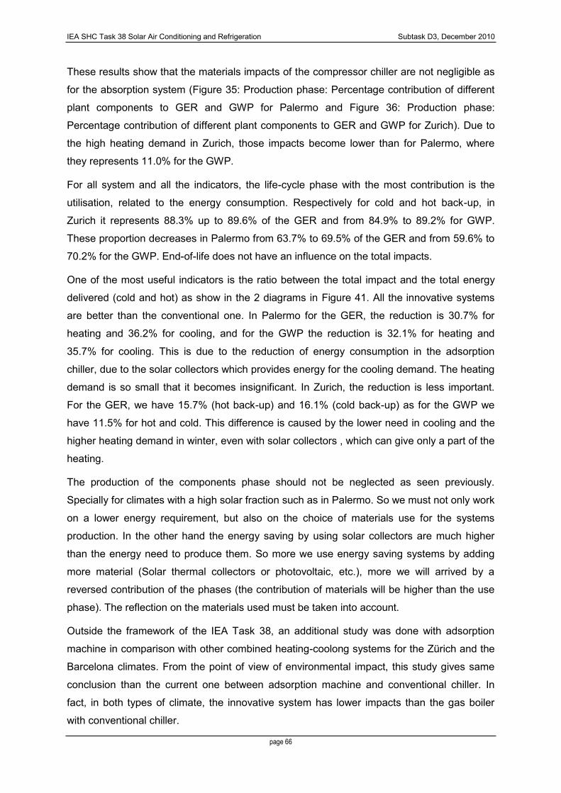
IEA SHC Task 38 Solar Air Conditioning and Refrigeration Subtask D3, December 2010
page 66
These results show that the materials impacts of the compressor chiller are not negligible as
for the absorption system (Figure 35: Production phase: Percentage contribution of different
plant components to GER and GWP for Palermo and Figure 36: Production phase:
Percentage contribution of different plant components to GER and GWP for Zurich). Due to
the high heating demand in Zurich, those impacts become lower than for Palermo, where
they represents 11.0% for the GWP.
For all system and all the indicators, the life-cycle phase with the most contribution is the
utilisation, related to the energy consumption. Respectively for cold and hot back-up, in
Zurich it represents 88.3% up to 89.6% of the GER and from 84.9% to 89.2% for GWP.
These proportion decreases in Palermo from 63.7% to 69.5% of the GER and from 59.6% to
70.2% for the GWP. End-of-life does not have an influence on the total impacts.
One of the most useful indicators is the ratio between the total impact and the total energy
delivered (cold and hot) as show in the 2 diagrams in Figure 41. All the innovative systems
are better than the conventional one. In Palermo for the GER, the reduction is 30.7% for
heating and 36.2% for cooling, and for the GWP the reduction is 32.1% for heating and
35.7% for cooling. This is due to the reduction of energy consumption in the adsorption
chiller, due to the solar collectors which provides energy for the cooling demand. The heating
demand is so small that it becomes insignificant. In Zurich, the reduction is less important.
For the GER, we have 15.7% (hot back-up) and 16.1% (cold back-up) as for the GWP we
have 11.5% for hot and cold. This difference is caused by the lower need in cooling and the
higher heating demand in winter, even with solar collectors , which can give only a part of the
heating.
The production of the components phase should not be neglected as seen previously.
Specially for climates with a high solar fraction such as in Palermo. So we must not only work
on a lower energy requirement, but also on the choice of materials use for the systems
production. In the other hand the energy saving by using solar collectors are much higher
than the energy need to produce them. So more we use energy saving systems by adding
more material (Solar thermal collectors or photovoltaic, etc.), more we will arrived by a
reversed contribution of the phases (the contribution of materials will be higher than the use
phase). The reflection on the materials used must be taken into account.
Outside the framework of the IEA Task 38, an additional study was done with adsorption
machine in comparison with other combined heating-coolong systems for the Zürich and the
Barcelona climates. From the point of view of environmental impact, this study gives same
conclusion than the current one between adsorption machine and conventional chiller. In
fact, in both types of climate, the innovative system has lower impacts than the gas boiler
with conventional chiller.

IEA SHC Task 38 Solar Air Conditioning and Refrigeration Subtask D3, December 2010
page 67
Like the previous chapter about absorption chiller, some payback indexes (EPT, EMPT and
ERR) have been calculated. Table 26: Payback indexes for the case studies shows the figures
of the three indexes for systems using the adsorption machine.
Table 26: Payback indexes for the case studies
EPT EMPT ERR year year Palermo Hot BU 9.31 6.03 2.25 Palermo Cold BU 9.25 8.92 2.31 Zurich Hot BU 8.87 8.60 2.37 Zurich Cold BU 9.30 10.63 2.30
The indexes have been calculated taking into account the cumulative energy demand of the
innovative system including from the construction to the end of life of the systems.
The EPT (Figure 42:) is defined as the use time during which the system must work to
produce as much Energy as it requires for its production and disposal.
Energy Payback Time (years)
9.61
9.209.569.67
0.0
1.0
2.0
3.0
4.0
5.0
6.0
7.0
8.0
9.0
10.0
Palermo Hot BU Palermo Cold BU Zurich Hot BU Zurich Cold BU
Year
Figure 42: EPT for Adsorption Solar Cooling systems with hot and cold back-up
Zurich figures are slightly lower than for Palermo (less than 5%).
- EMPT and ERR are two other indicators than can be used to compare the different
systems.
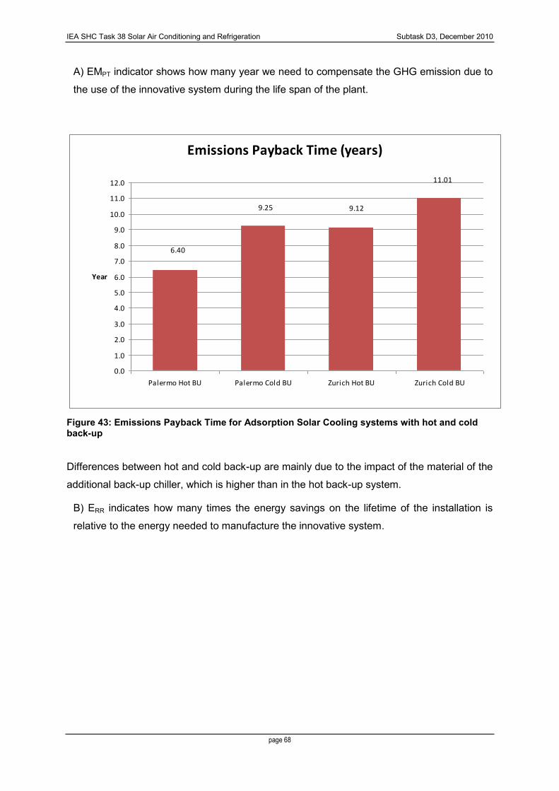
IEA SHC Task 38 Solar Air Conditioning and Refrigeration Subtask D3, December 2010
page 68
A) EMPT indicator shows how many year we need to compensate the GHG emission due to
the use of the innovative system during the life span of the plant.
Emissions Payback Time (years)
6.40
9.25 9.12
11.01
0.0
1.0
2.0
3.0
4.0
5.0
6.0
7.0
8.0
9.0
10.0
11.0
12.0
Palermo Hot BU Palermo Cold BU Zurich Hot BU Zurich Cold BU
Year
Figure 43: Emissions Payback Time for Adsorption Solar Cooling systems with hot and cold back-up
Differences between hot and cold back-up are mainly due to the impact of the material of the
additional back-up chiller, which is higher than in the hot back-up system.
B) ERR indicates how many times the energy savings on the lifetime of the installation is
relative to the energy needed to manufacture the innovative system.

IEA SHC Task 38 Solar Air Conditioning and Refrigeration Subtask D3, December 2010
page 69
Energy Return Ratio
2.25 2.312.37 2.30
0.0
0.5
1.0
1.5
2.0
2.5
3.0
Palermo Hot BU Palermo Cold BU Zurich Hot BU Zurich Cold BU
Year
Figure 44: ERR for Adsorption Solar Cooling systems with hot and cold back-up
In all the cases the results are satisfactory while the systems give back from more than 2
times the energy expenditure for their construction and disposal useful for the difference
between innovative and conventional system. As for the EPT, differences are not relevant
between all systems, less than 5%.

IEA SHC Task 38 Solar Air Conditioning and Refrigeration Subtask D3, December 2010
page 70
3.2 Solar DEC vs Conventional AHU: results from the operation phase of a plant in Palermo, Italy (DREAM)
The solar assisted DEC systems can be included in the product category of the ―Energy
Using Products‖ [Directive 2005/32/EC]. In this context, the operating phase cover a key-role
and it has to be investigated more in detail. The case study plant of the DREAM is already
operative and the collected data can be used to extrapolate general considerations about the
life-cycle impact about the system‘s operation.
Table 27: Monitored and estimated consumptions
Solar DEC - DREAM Conventional System
Electricity [kWh] LPG [kWh] Electricity [kWh] LPG [kWh]
Jan 530 213 519 816 Feb 479 574 466 1217
Mar
Apr
May
Jun (*) 1559 623
Jul 2207 2987 1328
Aug 2099 2641 1021
Sep 1411 1559 623
Oct
Nov
Dec 554 515 536 1268
Total 8691 1302 10267 6897
* Missing data
As first step, the analysis of the DREAM focuses on the assessment of impacts and benefits
related to the operating phase. Table 27 shows a comparison among the consumptions of
the experimental solar DEC and of a replaceable conventional system that operates under
the same operating conditions. Consumptions include the global electricity utilized by all the
system components (mainly chiller, pumps and fans), and the Liquid Petroleum Gas2 (LPG)
consumed by the auxiliary heating system.
Monitored data refer to the testing period (May 2008 – March 2009). Data about June 2008
are missing due to system start up problems.
2 At the time of the compilation of table 1LPG was used to fire the gas boiler. After, it was substitutes with
natural gas.

IEA SHC Task 38 Solar Air Conditioning and Refrigeration Subtask D3, December 2010
page 71
These data have been implemented into SimaPro software for the calculation of synthetic
environmental indexes. The analysis aims at assessing the energy and environmental
benefits related to the use of the experimental plants. Obtained results are however strictly
depending on the input eco-profiles of energy sources for the life-cycle inventory.
A preliminary discussion about key-issues of such life-cycle analysis has been following
synthesized:
- Energy mix: electricity is the largest energy input of the studied system. It is also
responsible of large environmental impacts strictly depending on the ―energy mix‖, meaning
the set of different processes and plants utilized for the electricity production. The choice of a
reliable electricity mix weights significantly on the final results and net benefits, and it has to
be carefully checked. In the studied context, the Italian national energy mix is based mainly
on thermoelectric generation systems (oil and gas fired plants) and imports from other
countries. The Sicilian regional mix, instead, is based by thermoelectric plants with a
significant presence of hydroelectric plants and wind farms. It could be possible even to refer
to an average international ―energy mix‖ that refers to an average European production. Data
about the Italian and the average European3 ―electricity mix‖ are included into Ecoinvent
database, while the eco-profile of the regional mix is missing. It has been therefore
calculated starting from data about the regional electricity production4 and the specific eco-
profiles per generating plant (included in the Ecoinvent database).
- LPG (Liquefied Petroleum Gas): it is utilized to fire a conventional gas boiler employed as
auxiliary system during the winter-time. The considered conventional system utilizes also
LPG in the summer for the post-heating in the air treatment unit. The Ecoinvent database
does not include the eco-profile of the LPG boiler.
Therefore, it has been carried out a reference analysis about the available data. The
acquired eco-profiles are:
o LPG fired in industrial equipments, concerning average USA technology in the late
1990‘s [Franklin, 1998];
o Derived data from the combustion of hydrocarbons (considering LPG as a mix of 60%
propane and 40% butane). Impacts related to the hydrocarbon use and production
refer to ―The Boustead Model‖, for the Italian context in the 2000‘s.
3 Average production of electricity in the UCTE (Union for the Co-ordination of Transmission of Electricity), concerning 24 European countries and 36 national operators for the electricity production. 4 From the Sicilian Regional Energy Plan (data from 2005), it resulted that in Sicily the electricity production is so subdivided: fossil fuels fired thermoelectric 83.1 %; hydropower 11.9 %; other renewable 5%.

IEA SHC Task 38 Solar Air Conditioning and Refrigeration Subtask D3, December 2010
page 72
- Useful life: the life length is another basic parameter that influences the LCA results.
Generally eco-profiles of products are improved extending the useful lifetime; but for Energy
Using Products, a loss in the energy efficiency could compromise the related benefits. At this
stage it is difficult to state the lifetime of the experimental system, being the operating time
too small and being the plant constituted by several different components with different
useful life. From a survey about the characteristics of system‘s components, it is expected an
average life of 20 years, but this value could have a ±20% variation.
Following these considerations, it has been decided to proceed to a scenario analysis in
order to define a ―base-case‖ scenario to which compare different alternatives concerning the
above key issues. This Scenario 0 supposes:
- To assess impacts due to electricity considering the national energy mix;
- To assess impacts due to LPG consumption considering the derived gas mix;
- To consider 20 years useful time;
- To use monitored data without modifies over the time due to the efficiency. In order
to allow the extrapolation of the results in a life-cycle perspective, monthly
consumptions of June have been assumed equal to September. This assessment is
realistic, being the average weather conditions of the two months similar.
Successively, Scenario 0 has been compare with the following alternative scenarios:
- Scenario 1: impacts related to electricity are assessed considering different energy
mix (national and regional);
- Scenario 2: Impacts related to LPG combustions are related to a different available
eco-profile;
- Scenario 3: Due to efficiency losses, energy consumptions of DEC are supposed to
grow constantly, arriving to a +20% increase of consumption at the last operating
year;
- Scenario 4: based on the above hypothesis of Scenario 3, lifetime is furthermore
considered to vary from 16 to 24 years. In the longest lifetime scenario, it is
expected that during the last 4 operating years, the efficiency will further decrease
with a yearly increase of the energy consumptions.
- Scenario 5: Impacts due to some innovative components are included in the
calculation of the environmental indexes of the ―base- case‖ (Scenario 0).
Results of scenarios are following described.
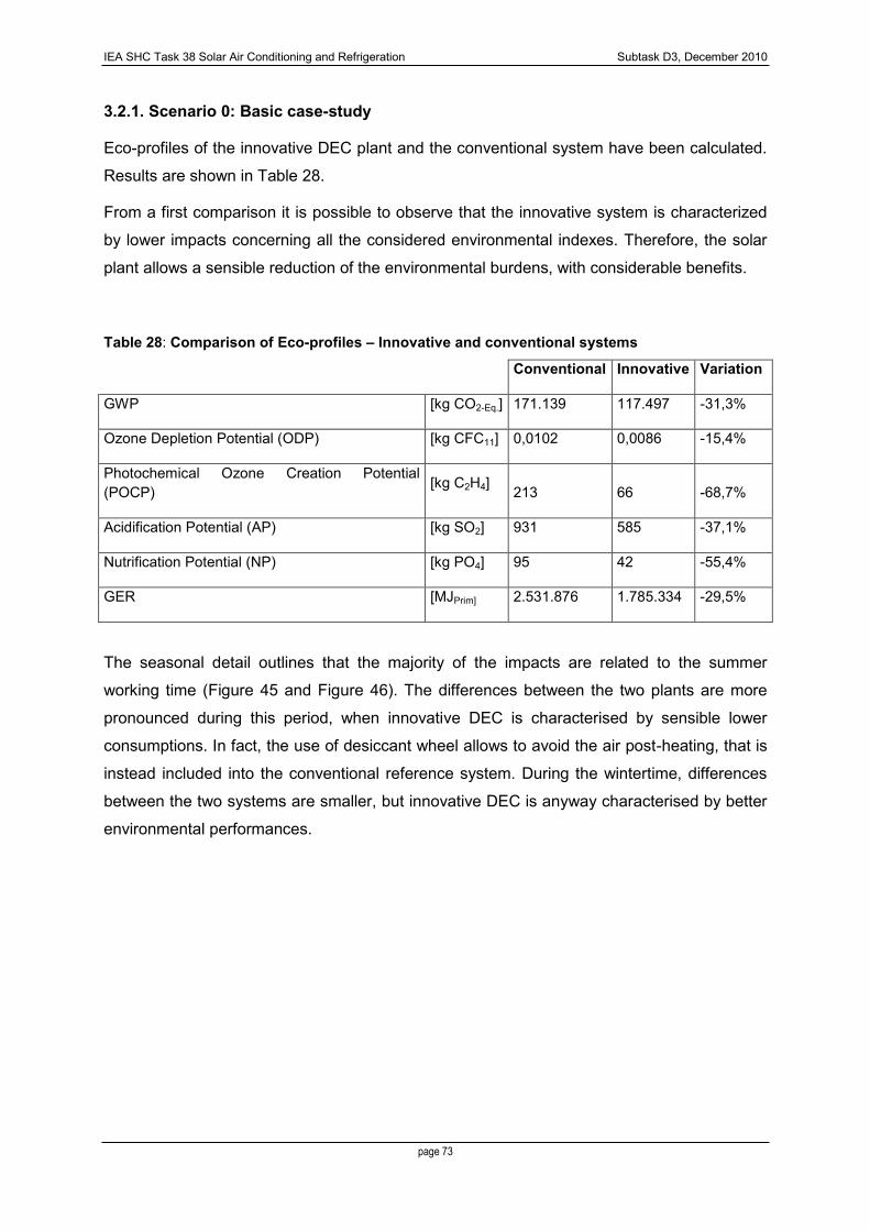
IEA SHC Task 38 Solar Air Conditioning and Refrigeration Subtask D3, December 2010
page 73
3.2.1. Scenario 0: Basic case-study
Eco-profiles of the innovative DEC plant and the conventional system have been calculated.
Results are shown in Table 28.
From a first comparison it is possible to observe that the innovative system is characterized
by lower impacts concerning all the considered environmental indexes. Therefore, the solar
plant allows a sensible reduction of the environmental burdens, with considerable benefits.
Table 28: Comparison of Eco-profiles – Innovative and conventional systems
Conventional Innovative Variation
GWP [kg CO2-Eq.] 171.139 117.497 -31,3%
Ozone Depletion Potential (ODP) [kg CFC11] 0,0102 0,0086 -15,4%
Photochemical Ozone Creation Potential (POCP) [kg C2H4] 213 66 -68,7%
Acidification Potential (AP) [kg SO2] 931 585 -37,1%
Nutrification Potential (NP) [kg PO4] 95 42 -55,4%
GER [MJPrim] 2.531.876 1.785.334 -29,5%
The seasonal detail outlines that the majority of the impacts are related to the summer
working time (Figure 45 and Figure 46). The differences between the two plants are more
pronounced during this period, when innovative DEC is characterised by sensible lower
consumptions. In fact, the use of desiccant wheel allows to avoid the air post-heating, that is
instead included into the conventional reference system. During the wintertime, differences
between the two systems are smaller, but innovative DEC is anyway characterised by better
environmental performances.

IEA SHC Task 38 Solar Air Conditioning and Refrigeration Subtask D3, December 2010
page 74
Figure 45: Comparison of seasonal impacts of the considered systems (GER)
Figure 46: Comparison of seasonal impacts of the considered systems (GWP)
A further detail concerned the subdivision about the used energy sources (Figure 47 and
Figure 48). It is possible to observe that the majority of the impacts are related to the use of
electricity, due to the large consumptions and the eco-profile of the electricity production in
the Italian context. The incidence of LPG is marginal, especially in the innovative system.
The environmental impacts have been therefore detailed about each system‘s components,
in order to identify the most impacting elements. Consumptions of DEC have been
subdivided into the following components:
- Auxiliary system: it encloses electrical consumption for pumps and actuators;
GER - Comparison of plants (seasonal detail)
0
500.000
1.000.000
1.500.000
2.000.000
2.500.000
3.000.000
[MJprim]
Summer 1.976.934 1.379.977 596.957
Winter 554.941 405.357 149.584
Conventional Innovative Net Benefits
GWP- Comparison of plants (seasonal detail)
-
40.000
80.000
120.000
160.000
200.000
[kgCO2eq]
Summer 132.031 89.921 42.110
Winter 27.576 39.108 -11.532
Conventional Innovative Net Benefits

IEA SHC Task 38 Solar Air Conditioning and Refrigeration Subtask D3, December 2010
page 75
- AHU - Air Handling Unit: it encloses electrical consumption for fans, humidifiers,
electrical engines of rotors;
- Radiant ceiling: it encloses electrical consumption for pumps and actuators;
- Chiller;
- Gas boiler, fired by LPG.
Figure 47: Comparison of impacts due to energy sources use (GER)
GWP (Energy source detail)
0
25.000
50.000
75.000
100.000
125.000
150.000
175.000
200.000
[kgC
O2
eq]
Electricity 129.531 109.643 19.888
LPG 41.609 7.854 33.754
Conventional Innovative Net Benefits
Figure 48: Comparison of GWP impacts due to energy sources use
The analysis (Figure 49 and Figure 50) shows that, concerning for example the GER and the
GPW indexes, the chiller and AHU are the most impacting components, and together they
GER - Comparison of plants (Energy source detail)
0
500.000
1.000.000
1.500.000
2.000.000
2.500.000
3.000.000
[MJprim]
Electricity 1.987.852 1.682.642 305.211
LPG 544.023 102.693 441.331
Conventional Innovative Net Benefits

IEA SHC Task 38 Solar Air Conditioning and Refrigeration Subtask D3, December 2010
page 76
are responsible of about 80% of the overall greenhouse gas emissions and PE consumption.
Similar results have been observed for the other impact categories.
Figure 49: Comparison of impacts related to system components (GER)
Figure 50: Comparison of impacts related to system components (GWP)
GER: Components detail
0
100.000
200.000
300.000
400.000
500.000
600.000
700.000
800.000
900.000
1.000.000
Auxiliary components
AHU Radiant ceiling Chiller Boiler (LPG)
[MJprim]
GWP: Components detail
0
10.000
20.000
30.000
40.000
50.000
60.000
Auxiliary components
AHU Radiant ceiling Chiller Boiler (LPG)
[kgCO2eq]

IEA SHC Task 38 Solar Air Conditioning and Refrigeration Subtask D3, December 2010
page 77
3.2.2 Scenario 1: Electricity mix.
The previous analysis confirmed the key role of the electricity consumption in the DEC
system eco-profile. A more detailed analysis about impacts related to electricity is therefore
necessary. Eco-profile of different electricity production mix have been implemented, as
described in paragraph 3.2. The new results about of the eco-profiles of the innovative
system are shown in Table 29.
Table 29: Changes of the eco-profile of the innovative systems due to different electricity mix
National En. Mix Regional En. Mix International En. Mix
(Scenario 0) Values
Variation respect to Scenario 0
Values
Variation respect to Scenario 0
GWP [kg CO2-Eq.] 117.497 112.523 -4,2%
111.493 -5,1%
Ozone Depletion Potential (ODP) [kg CFC11]
0,009 0,011 33,7%
0,004 -48,6%
Photochemical Ozone Creation Potential (POCP)
[kg C2H4] 66 57 -13,9%
56 -15,0%
Acidification Potential (AP) [kg SO2]
585 181 -69,1%
530 -9,4%
Nutrification Potential (NP) [kg PO4]
42 28 -34,7%
35 -16,8%
GER [MJPrim] 1.785.334 1.907.952 6,9%
2.121.334 18,8%
The estimated variations are often significant or very significant. The smallest differences are
related to the GWP and the GER indexes. It has been identified that the GWP varies from
111·103 kg CO2-Eq. to 117·103 kg CO2-Eq, while the GER (Figure 51) varies from 1.78 106
MJPrim to 2.1 106 MJPrim.
Very significant changes are instead related to the AP and the ODP indexes. This last can be
related to the very small values previously detected. Therefore, even small changes into the
calculated values can cause large variations. The ODP values are, however always almost
negligible.

IEA SHC Task 38 Solar Air Conditioning and Refrigeration Subtask D3, December 2010
page 78
The adoption of regional or international energy mixes causes contrasting effects, increasing
the values of GER, but decreasing the other impacts indicators.
The current scenario confirms the large variability due to electricity data. Anyway, national
energy mix still represents the most reliable input data, being the international average
electricity mix small fitting with the current case study, and being the eco-profile of the
regional electricity mix an assessment extrapolated from reference data.
GER - Comparison of Scenarios
-
500.000
1.000.000
1.500.000
2.000.000
2.500.000
National En.
Mix
Regional En.
Mix
International
En. Mix
[MJ P
rim
]
Figure 51: Comparison of GER values due to different electricity eco-profiles
3.2.3 Scenario 2: LPG eco-profiles
A further analysis about impacts related to LPG combustion has been carried out. Impacts
estimated due to the assessed LPG eco-profile have been compared to the impacts
assessed by Franklin Ltd for an average plant in the USA. Scenario results are shown in
Table 30 and Figure 52.
Results showed that the incidence of LPG eco-profile changes is minor into GER and GWP
indexes, especially concerning the innovative plant. Larger variations are instead detected
into AP, POPC and NP indexes.
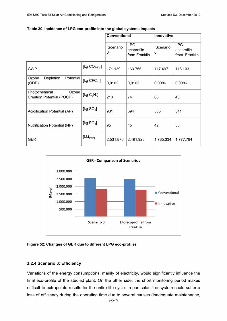
IEA SHC Task 38 Solar Air Conditioning and Refrigeration Subtask D3, December 2010
page 79
Table 30: Incidence of LPG eco-profile into the global systems impacts
Conventional Innovative
Scenario 0
LPG ecoprofile from Franklin
Scenario 0
LPG ecoprofile from Franklin
GWP [kg CO2-Eq.] 171.139
163.755
117.497
116.103
Ozone Depletion Potential (ODP) [kg CFC11]
0,0102
0,0102
0,0086
0,0086
Photochemical Ozone Creation Potential (POCP) [kg C2H4]
213
74
66
40
Acidification Potential (AP) [kg SO2]
931
694
585
541
Nutrification Potential (NP) [kg PO4] 95
45
42
33
GER [MJPrim] 2.531.876
2.491.928
1.785.334
1.777.794
GER - Comparison of Scenarios
-
500.000
1.000.000
1.500.000
2.000.000
2.500.000
3.000.000
Scenario 0 LPG ecoprofile from
Franklin
[MJ P
rim
]
Conventional
Innovative
Figure 52: Changes of GER due to different LPG eco-profiles
3.2.4 Scenario 3: Efficiency
Variations of the energy consumptions, mainly of electricity, would significantly influence the
final eco-profile of the studied plant. On the other side, the short monitoring period makes
difficult to extrapolate results for the entire life-cycle. In particular, the system could suffer a
loss of efficiency during the operating time due to several causes (inadequate maintenance,
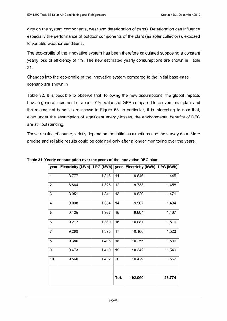
IEA SHC Task 38 Solar Air Conditioning and Refrigeration Subtask D3, December 2010
page 80
dirty on the system components, wear and deterioration of parts). Deterioration can influence
especially the performance of outdoor components of the plant (as solar collectors), exposed
to variable weather conditions.
The eco-profile of the innovative system has been therefore calculated supposing a constant
yearly loss of efficiency of 1%. The new estimated yearly consumptions are shown in Table
31.
Changes into the eco-profile of the innovative system compared to the initial base-case
scenario are shown in
Table 32. It is possible to observe that, following the new assumptions, the global impacts
have a general increment of about 10%. Values of GER compared to conventional plant and
the related net benefits are shown in Figure 53. In particular, it is interesting to note that,
even under the assumption of significant energy losses, the environmental benefits of DEC
are still outstanding.
These results, of course, strictly depend on the initial assumptions and the survey data. More
precise and reliable results could be obtained only after a longer monitoring over the years.
Table 31: Yearly consumption over the years of the innovative DEC plant
year Electricity [kWh] LPG [kWh] year Electricity [kWh] LPG [kWh]
1 8.777 1.315 11 9.646 1.445
2 8.864 1.328 12 9.733 1.458
3 8.951 1.341 13 9.820 1.471
4 9.038 1.354 14 9.907 1.484
5 9.125 1.367 15 9.994 1.497
6 9.212 1.380 16 10.081 1.510
7 9.299 1.393 17 10.168 1.523
8 9.386 1.406 18 10.255 1.536
9 9.473 1.419 19 10.342 1.549
10 9.560 1.432 20 10.429 1.562
Tot. 192.060 28.774

IEA SHC Task 38 Solar Air Conditioning and Refrigeration Subtask D3, December 2010
page 81
Table 32: Eco-profile changes due to assumptions about efficiency loss
Scenario 0 Efficiency scenario
GWP [kg CO2-Eq.] 117.497 129.834
Ozone Depletion Potential (ODP) [kg CFC11] 0,009 0,009
Photochemical Ozone Creation Potential (POCP) [kg C2H4] 66 73
Acidification Potential (AP) [kg SO2] 585 647
Nutrification Potential (NP) [kg PO4] 42 47
GER [MJPrim] 1.785.334 1.972.793
GER - Comparison of Scenarios
-
500.000
1.000.000
1.500.000
2.000.000
2.500.000
3.000.000
Scenario 0 Efficiency loss scenario
[MJ P
rim
]
Conventionalplant
Innovativeplant
Net Benefit
Figure 53: Comparison of GER index from different scenarios
3.2.5 Scenario 4: Lifetime
The length of the operating time is another key parameter in the life-cycle balance of the
plants. It has been decided to make different hypotheses about the useful life, varying it from
16 to 24 years. This scenario have been coupled with the previous one, supposing a
constant +1% yearly increase of the energy consumptions until the 20th year, and,
successively, a +2.5% increase in the last 4 years.
The impacts have been still compared to a conventional system supposing its efficiency to be
not decreased over the time. This choice is based on the following assumptions:
- The assessment of the consumptions of the conventional system is an ―average‖
data, based on simulating tools that already take into account the average
performances of the plant over the years. The estimation of the life-cycle

IEA SHC Task 38 Solar Air Conditioning and Refrigeration Subtask D3, December 2010
page 82
consumptions of the DEC system is instead based on the monitored data that,
currently, refer only to the first operating year;
- Efficiency losses are ascribed only to the innovative system, in order to evaluate its
performances even in a ―pessimistic‖ scenario.
The yearly consumptions of the innovative plant are shown in Table 33. Environmental
impacts are synthesized in Table 34.
Table 33: Yearly consumption over the time (scenarios at 16, 20 and 24 years)
year Electricity [kWh]
LPG [kWh] year Electricity
[kWh] LPG [kWh] year Electricity
[kWh] LPG [kWh]
1 8.777 1.315 9 9.473
1.419 17 10.168 1.523
2 8.864 1.328 10 9.560
1.432 18 10.255 1.536
3 8.951 1.341 11 9.646
1.445 19 10.342 1.549
4 9.038 1.354 12 9.733
1.458 20 10.429 1.562
5 9.125 1.367 13 9.820
1.471 21 10.646
1.595
6 9.212 1.380
14 9.907 1.484
22 10.863 1.628
7 9.299 1.393 15 9.994
1.497 23 11.080 1.660
8 9.386 1.406 16 10.081
1.510 24 11.298 1.693
Tot. 16 years 150.867
22.603 Tot. 20 years 192.060
28.774 Tot. 24 years 235.947
35.349
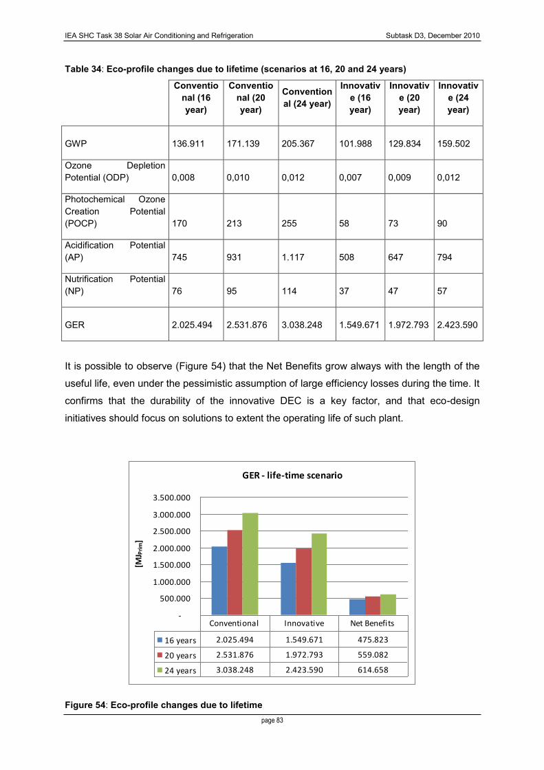
IEA SHC Task 38 Solar Air Conditioning and Refrigeration Subtask D3, December 2010
page 83
Table 34: Eco-profile changes due to lifetime (scenarios at 16, 20 and 24 years)
Conventional (16 year)
Conventional (20 year)
Conventional (24 year)
Innovative (16 year)
Innovative (20 year)
Innovative (24 year)
GWP 136.911
171.139
205.367
101.988
129.834
159.502
Ozone Depletion Potential (ODP)
0,008
0,010
0,012
0,007
0,009
0,012
Photochemical Ozone Creation Potential (POCP)
170
213
255
58
73
90
Acidification Potential (AP)
745
931
1.117
508
647
794
Nutrification Potential (NP)
76
95
114
37
47
57
GER 2.025.494
2.531.876
3.038.248
1.549.671
1.972.793
2.423.590
It is possible to observe (Figure 54) that the Net Benefits grow always with the length of the
useful life, even under the pessimistic assumption of large efficiency losses during the time. It
confirms that the durability of the innovative DEC is a key factor, and that eco-design
initiatives should focus on solutions to extent the operating life of such plant.
GER - life-time scenario
-
500.000
1.000.000
1.500.000
2.000.000
2.500.000
3.000.000
3.500.000
[MJ P
rim
]
16 years 2.025.494 1.549.671 475.823
20 years 2.531.876 1.972.793 559.082
24 years 3.038.248 2.423.590 614.658
Conventional Innovative Net Benefits
Figure 54: Eco-profile changes due to lifetime
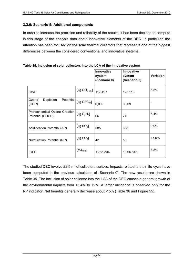
IEA SHC Task 38 Solar Air Conditioning and Refrigeration Subtask D3, December 2010
page 84
3.2.6: Scenario 5: Additional components
In order to increase the precision and reliability of the results, it has been decided to compute
in this stage of the analysis data about innovative elements of the DEC. In particular, the
attention has been focused on the solar thermal collectors that represents one of the biggest
differences between the considered conventional and innovative systems.
Table 35: Inclusion of solar collectors into the LCA of the innovative system
Innovative system (Scenario 0)
Innovative system (Scenario 5)
Variation
GWP [kg CO2-Eq.] 117.497
125.113 6,5%
Ozone Depletion Potential (ODP)
[kg CFC11] 0,009
0,009
-
Photochemical Ozone Creation Potential (POCP) [kg C2H4]
66
71 6,4%
Acidification Potential (AP) [kg SO2] 585
638 9,0%
Nutrification Potential (NP) [kg PO4] 42
50 17,5%
GER [MJPrim] 1.785.334
1.906.813 6,8%
The studied DEC involve 22.5 m2 of collectors surface. Impacts related to their life-cycle have
been computed in the previous calculation of ―Scenario 0‖. The new results are shown in
Table 35. The inclusion of solar collector into the LCA of the DEC causes a general growth of
the environmental impacts from +6.4% to +9%. A larger incidence is observed only for the
NP indicator. Net benefits generally decrease about -15% (Table 36 and Figure 55).
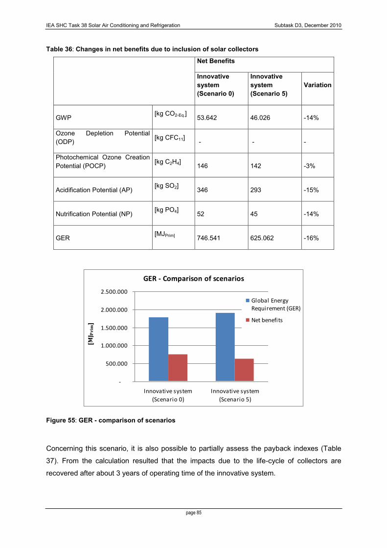
IEA SHC Task 38 Solar Air Conditioning and Refrigeration Subtask D3, December 2010
page 85
Table 36: Changes in net benefits due to inclusion of solar collectors
Net Benefits
Innovative system (Scenario 0)
Innovative system (Scenario 5)
Variation
GWP [kg CO2-Eq.] 53.642
46.026 -14%
Ozone Depletion Potential (ODP) [kg CFC11] - - -
Photochemical Ozone Creation Potential (POCP) [kg C2H4]
146
142 -3%
Acidification Potential (AP) [kg SO2]
346
293 -15%
Nutrification Potential (NP) [kg PO4] 52
45 -14%
GER [MJPrim] 746.541
625.062 -16%
GER - Comparison of scenarios
-
500.000
1.000.000
1.500.000
2.000.000
2.500.000
Innovative system
(Scenario 0)
Innovative system
(Scenario 5)
[MJ Prim]
Global EnergyRequirement (GER)
Net benefits
Figure 55: GER - comparison of scenarios
Concerning this scenario, it is also possible to partially assess the payback indexes (Table
37). From the calculation resulted that the impacts due to the life-cycle of collectors are
recovered after about 3 years of operating time of the innovative system.
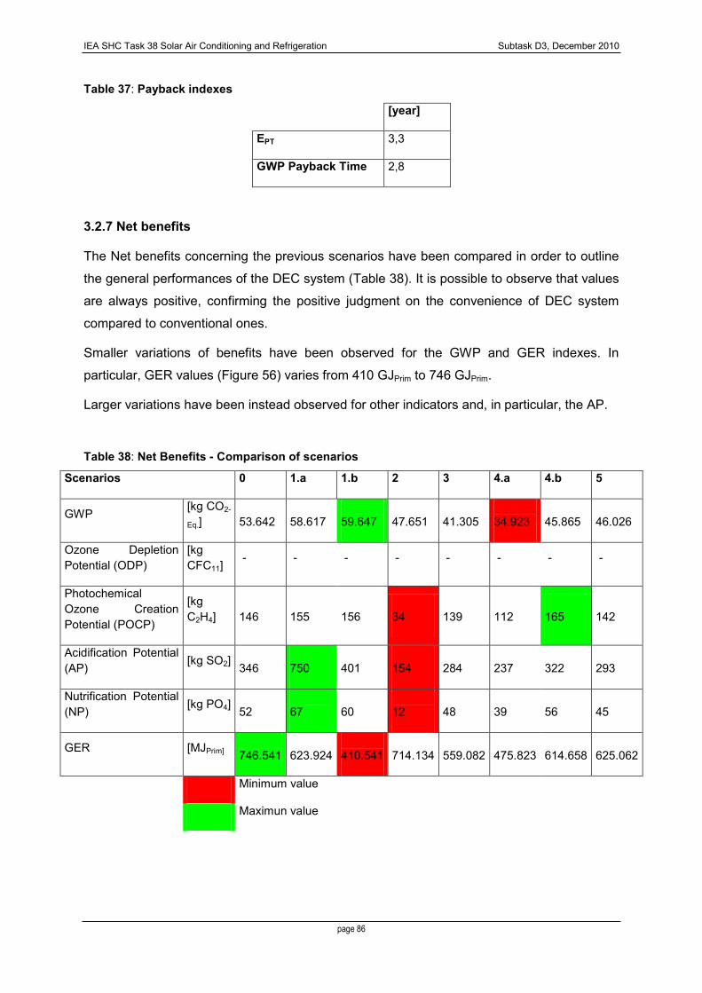
IEA SHC Task 38 Solar Air Conditioning and Refrigeration Subtask D3, December 2010
page 86
Table 37: Payback indexes
[year]
EPT 3,3
GWP Payback Time 2,8
3.2.7 Net benefits
The Net benefits concerning the previous scenarios have been compared in order to outline
the general performances of the DEC system (Table 38). It is possible to observe that values
are always positive, confirming the positive judgment on the convenience of DEC system
compared to conventional ones.
Smaller variations of benefits have been observed for the GWP and GER indexes. In
particular, GER values (Figure 56) varies from 410 GJPrim to 746 GJPrim.
Larger variations have been instead observed for other indicators and, in particular, the AP.
Table 38: Net Benefits - Comparison of scenarios
Scenarios 0 1.a 1.b 2 3 4.a 4.b 5
GWP [kg CO2-
Eq.] 53.642
58.617
59.647
47.651
41.305
34.923
45.865
46.026
Ozone Depletion Potential (ODP)
[kg CFC11]
- - - - - - - -
Photochemical Ozone Creation Potential (POCP)
[kg C2H4]
146
155
156
34
139
112
165
142
Acidification Potential (AP) [kg SO2]
346
750
401
154
284
237
322
293
Nutrification Potential (NP) [kg PO4]
52
67
60
12
48
39
56
45
GER [MJPrim] 746.541
623.924
410.541
714.134
559.082
475.823
614.658
625.062
Minimum value
Maximun value

IEA SHC Task 38 Solar Air Conditioning and Refrigeration Subtask D3, December 2010
page 87
GER benefits - Comparison of Scenarios
-
100.000
200.000
300.000
400.000
500.000
600.000
700.000
800.000
Scenario
0
Scenario
1.a
Scenario
1.b
Scenario
2
Scenario
3
Scenario
4.a
Scenario
4.b
Scenario
5
[MJ P
rim
]
Figure 56: GER Benefits- Comparison of scenarios
3.2.8 Conclusions and expected progress
The analysis on the operating phase of the innovative system showed the great energy and
environmental convenience of this technology. Impacts due to the DEC plant are about one
third lower compared to those related to a conventional system. From the analysis of
different alternative scenarios, it resulted that:
- GWP and GER indexes are generally affected by small variations due to
hypotheses changes;
- Other indicators (as AP, NP and POPC) have, instead large variations, especially
due to changes into electricity or LPG combustion eco-profiles;
- ODP index has generally very low or negligible values;
- The longer is the operating time of the DEC, the larger are the Net benefits, even
accounting a continuously efficiency loss, up to a +30% growth of the energy
consumptions after 24 years;
- The analysis of innovative components of the plants have not been included into the
environmental balances, due to data availability and to the project scopes, aiming at
assessing the net benefits of DEC system compared to a conventional ―reference‖
plant. For this reason, it is important to focus the attention only on the exclusive
innovative elements, meaning the element contained in the DEC system and
missing in the reference system. A first step on this direction has been made,
including in the computation the life-cycle impacts of solar thermal collectors. Their

IEA SHC Task 38 Solar Air Conditioning and Refrigeration Subtask D3, December 2010
page 88
inclusion causes a reduction of net benefits of about 15%, with a payback time of
about 3 years.

IEA SHC Task 38 Solar Air Conditioning and Refrigeration Subtask D3, December 2010
page 89
4. Conclusions
LCA of solar cooling plants has been performed according to the LCA standards of the ISO
14040 series. The research aimed to evaluate and compare the energy and environmental
performances of solar cooling systems with traditional plants.
Four different cases have been investigated in order to assess the performances of two
different technologies of thermally driven chillers (Absorption and Adsorption) applied in two
localities: Palermo (South Italy) and Zurich (Switzerland).
In addition two possible alternatives in the configurations according to the modality of back-
up of the solar cooling systems in summer operation (cold back-up and hot-back-up) have
been included.
The performances of these 4 systems has been compared to a conventional system with a
vapour compression chiller and a gas boiler.
A detailed LCA study was performed for the absorption (ABS) and adsorption (ADS) chillers,
that represent the main components of the two examined plants.
Comparing the eco-profiles of the ABS and the ADS chillers, the highest values of GER and
GWP are related to the first one. In detail GER and GWP for ABS chiller are, respectively, 28
GJ and 1524 kg CO2eq; for the second one are, respectively, 24 GJ and 1401 kg CO2eq.
The differences are principally due to the system boundaries: for ABS the energy use for the
fabrication of the chiller and the transport of the materials to the plant have been included, for
the
ADS where not because of lack of information. Also differences could be due to different
quantities of raw materials used in the production process.
For both chillers the main impacts on GER and GWP are due to the production phase.
The comparison of the eco-profiles of ABS and ADS plants showed that for both
configurations (hot and cold backup) the highest impacts are related to the absorption plant
(Figure 54). The differences are mainly observable in the use phase, that is responsible of
the main impacts during the life-cycle of both plants.
The impacts caused by the plants installed in Zurich are higher than those in Palermo, mainly
due to the higher energy consumption in the first one during the use phase.

IEA SHC Task 38 Solar Air Conditioning and Refrigeration Subtask D3, December 2010
page 90
0
200000
400000
600000
800000
1000000
1200000
1400000
1600000
ABS - HOT ADS - HOT ABS - COLD ADS - COLD
GJ
GER
Palermo
Zurich
0
10000
20000
30000
40000
50000
60000
70000
80000
90000
ABS - HOT ADS - HOT ABS - COLD ADS - COLD
kg
CO
2eq
GWP
Palermo
Zurich
Figure 54: Comparison of GER (MJ) and GWP for ABS and ADS plants
The innovative systems have been compared with the conventional one using three different
FUs: a solar cooling plant with absorption or adsorption chiller; 1 kW of power of the chiller; 1
kWh of energy produced by plant.
Analyzing the results it can be observed that the absorption plant has lower impacts than the
conventional one for all different FUs. The impacts of the adsorption plant result lower than
the conventional one; the only exception is represented by the choice of 1 kW of power of the
chiller as FU.
In order to assess the effective energy and environmental advantage related to the use of
innovative systems, the EPT, the ERR and the EMPT time have been calculated.
A summary of the results for both plants is shown in Figure 55.
4.30
2.25
3.84
2.31
4.99
2.37
4.59
2.30
0,00
1,00
2,00
3,00
4,00
5,00
6,00
ABS - HOT ADS - HOT ABS - COLD ADS - COLD
yea
rs
ERR
Palermo
Zurich
5.10
9.31
5.80
9.25
4.41
8.87
4.85
9.30
0,00
1,00
2,00
3,00
4,00
5,00
6,00
7,00
8,00
9,00
10,00
ABS - HOT ADS - HOT ABS - COLD ADS - COLD
yea
rs
EPT
Palermo
Zurich3.98
6.03 6.02
8.92
3.93
8.60
5.58
10.6
0,00
2,00
4,00
6,00
8,00
10,00
12,00
ABS - HOT ADS - HOT ABS - COLD ADS - COLD
yea
rs
EMPT
Palermo
Zurich
Figure 55: Comparison of EPT, EMPT and ERR for ABS and ADS plants

IEA SHC Task 38 Solar Air Conditioning and Refrigeration Subtask D3, December 2010
page 91
In general it can be said that results are almost fair. EPT ranges in all cases from 4.5 to 9.5
years. Emission paybacks ranges from 4 to 10.5 years. The systems which requires less
years to give back the energy needed for its construction, operation and disposal are the one
using ABS chillers.
In general, for the EPT:
- for a given climate and back-up typology: systems with ABS chillers performs better
than one with ADS chillers
- for a given system the colder the climate the lower the energy return
- for a given climate and chiller typology: the «hot back-up» is slightly better than the
«cold back-up» (with some exception)
and for the emissions:
- for a given climate and back-up typology: systems with ABS chillers performs better
than ones with ADS chillers
- for a given system with ABS chiller, the colder the climate the higher the emission
payback
- for a given system with ADS chiller, the colder the climate the higher the emission
payback
- for a given climate and chiller typology: the «hot back-up» is better than the «cold
back-up»
It is worth noting that the results obtained show good performances of almost all the
configurations form the environmental point of view. They can be used to show the net
environmental benefits related to SHC systems despite the larger amount of energy and
emissions related to their construction.
Anyway it must be stressed that although they are referred to the two case studies above
described, the study has demonstrated the possibility to apply LCA method to every solar
H/C system. New applications can be made for other systems by considering different sizes,
climate, loads, energy mix, emissions factors.

IEA SHC Task 38 Solar Air Conditioning and Refrigeration Subtask D3, December 2010
page 92
5. Bibliography
Ardente F, Beccali G, Cellura M, Lo Brano V, Life cycle analysis of solar thermal collector
(first part: life cycle inventory), First report of the International Energy Agency (IEA) - Task
27—Performance of solar facade, Subtask C—Project C1 environmental performance;
March 2003.
Ardente F., Beccali G., Cellura M., Lo Brano V., 2005, Life cycle assessment of a solar
thermal collector, Renewable Energy, 30, pp. 1031-1054
Battisti R., Corrado A., 2005a, Evaluation of technical improvements of photovoltaic systems
through life cycle assessment methodology, Energy, 30, pp. 952-967
Battisti R., Corrado A., 2005b, Environmental assessment of solar thermal collectors with
integrated water storage, Journal of Cleaner Production, 13, pp. 1295-1300
Bjorklund AE, Survey of approaches to improve reliability in LCA, Int J LCA 2002;7(2):64–72.
Boustead Consulting Ltd. 2001. Environmental database, ver. 4.4. Boustead Consulting, Ltd.,
Black Cottage, West Sussex, UK.
COMMISSION RECOMMENDATION of 10 July 2003 on ―Guidance for the implementation of
Regulation (EC) No 761/2001 of the European Parliament and of the Council allowing
voluntary participation by organizations in a Community eco-management and audit scheme
(EMAS) concerning the selection and use of environmental performance indicators‖.
2003/532/EC.
Directive 2005/32/EC establishing a framework for the setting of ecodesign requirements for
energy-using products and amending Council Directive 92/42/EEC and Directives 96/57/EC
and 2000/55/EC
Franklin Associates, Ltd. Franklin Database Manual, 1998AFNOR Association Française de
Frischknecht R., Jungbluth N., Althaus H.-J., Doka G., Dones R., Heck T., Hellweg S.,
Hischier R., Nemecek T., Rebitzer G. and Spielmann M. (2007) Overview and Methodology.
ecoinvent report No. 1, v2.0. Swiss Centre for Life Cycle Inventories, Dübendorf, CH.
Included in the software SimaPro ver. 7.1 (http://www.pre.nl/simapro/)
Garcìa-Valverde R., Miguel C., Martìnez-Bèjar R., Urbina A., 2009, Life cycle assessmnet
study of a 4.2 kWp stand-alone photovoltaic system, Solar Energy, 83, pp. 1434-1445
Kalogirou S. A., 2004, Environmental benefits of domestic solar energy sistems, Energy
Conversion and Management, 45, pp. 3075-3092
Kalogirou S., 2009, Thermal performance, economic and environmental life cycle analysis of
thermosiphon solar water heaters, Solar Energy, 83, pp. 39-48

IEA SHC Task 38 Solar Air Conditioning and Refrigeration Subtask D3, December 2010
page 93
Kannan R., Leong K.C., Osman R., Ho H.K., Tso C.P., 2006, Life cycle assessment study of
solar PV systems: An example of a 2.7 kWp distributed solar PV system in Singapore, Solar
Energy, 80, pp. 555-563
NORmalisation, XP P01010-1; Environmental quality of construction products - Information
concerning the environmental characteristics of construction products - Part 1 : methodology
and model of data declaration, April 2001
Heijungs R, Identification of key issues for further investigation in improving the reliability of
life-cycle assessments. Journal of Cleaner Production, 1996 Volume 4, Number 3-4, p.159.
Huijbregts M, Norris G, von Bahr B,. General framework to compare and develop methods
for uncertainty assessment in LCI, working paper from SETAC LCA workgroup on data
availability and data quality. 1999.
International Iron and Steel Industry, World Steel Life Cycle Inventory - Methodology Report -
1999/2000, Committee on Environmental Affairs, Brussels, October 2002.
ISO 14031. ―Environmental management - Environmental performance evaluation –
Guidelines―. 1999
ISO 14040. ―Environmental management - Life cycle assessment - Principles and
framework―. 2006.
ISO 14044. ―Environmental management -- Life cycle assessment -- Requirements and
guidelines‖. 2006.
ISO/TS 14048. ―Environmental management -- Life cycle assessment -- Data documentation
format―. 2006.
ISO 15686. Buildings and constructed assets—service life planning—part 1: general
principles. 2000.
Kemna R, van Elburg M, Li W, van Holsteijn R, Methodology Study Eco-design of Energy-
using Products - Final Report – MEEUP. Product Cases Report. Delft, 28.11.2005.
Kennedy, D J, Montgomery D C, Rollier D A and Keats J B , Data quality, Assessing input
data uncertainty in Life Cycle Assessment Inventory Models. In International Journal of Life
Cycle Assessment 2 (4) pp. 229-239, 1997.
Krűgher U, Arc Welding Processes: TIG, Plasma Arc, MIG. TALAT lecturer 4201. EEA-
European Aluminum Association, 1994.
Meier, M A, Eco-efficiency evaluation of waste gas purification systems in the chemical
industry. LCA documents vol 2. Ecomed, Landsberg, Germany 1997. ISBN 3-928379-54-2.
PRè-Product Ecology Consultants, 2006, SimaPro7.1 environmental database.
IEA SHC Task 38 Solar Air Conditioning and Refrigeration Subtask D3, December 2010
page 94
Rupp J, Koch L, Wiemkem E, Nienborg B, SorTech package solution, Description of the
package solution, project Solarcombi+, October 2009
Solanext Technical sheet, Absorption Cooling Technology. From website:www.solanext.com
SorTech Adsorption Chiller, Instruction and Installation Manual for ACS 08/ACS 15, July
2009
Swedish Environmental Management Council, Requirements for Environmental Product
Declaration, EPD – An Application of ISO TR 14025 Type III Environmental Declarations,
27/3/2000.
The International EPD Cooperation (IEC), Supporting Annexes for Environmental Product
Declarations, EPD, version 1.0 dated 2008-02-29
The Swiss Centre for life cycle inventories. Ecoinvent data v2.0.
Weidema, B and Suhr Wesnus M, Data quality management for life cycle inventories, an
example of using data quality indicators. Journal of .Cleaner Production, 1996 , Vol. 4, no. 3-
4, p. 167-174.
Wrisberg M N, A semi-quantitative approach for assessing data quality in LCA . Proceedings
7th Annual Meeting of SETAC-Europe, Amsterdam , April 6-10, 1997.
The International EPD Cooperation (IEC). General Programme instructions for
Environmental Product Declarations, EPD. version 1.0 dated 2008-02-29.
Van den Berg N W, Huppes G, Lindeijer E W, Van der Ven B L, Wrisberg M N, Quality
Assessment for LCA. CML Report 152 ISBN:

IEA SHC Task 38 Solar Air Conditioning and Refrigeration Subtask D3, December 2010
page 95
6. Annex 1 . DATA BASE OF LCIs OF EQUIPMENTS FOR SHC PLANTS
6.1 Solar thermal collectors (evacuated)
1. Product: Evacuated tube collectors (F.U.: 1 m2 of evacuated tube collectors)
2. Authors and reference: data published by Niels Jungbluth in Ecoinvent ver.2.0
3. Description of the product: Evacuated tube collectors for hot water production.
4. Product characteristics
Nominal power/surface/other: surface 1 m2
Measured/estimated yearly energy production and/or consumption:-
Information about the use phase: -
Information about the end-of-life phase: wastes as plastics, packaging, hazardous
wastes and others are incinerated. Glass and rock wool wastes are recovered.
5. Metadata
Age of the study: Materials data have been investigated for a collector produced
in 2002. Data for energy uses during production have been investigated for 2001.
System boundaries (production phase, use phase, end-of-life phase): data are
referred to the production of an evacuated tube collector in Northern-Ireland,
including materials and energy use of production, and disposal of the product at
the end of life.
Useful life-time: 25 years.
Cut-off rules: impacts related to transport of the solar thermal collectors from the
productive site to the utilization site and to the use phase are not included.
Allocation rules: -
Further details: -
Data Quality Assessment: input data of materials used to produce the solar
thermal collector have been collected using questionnaires.
Energy uses during production investigated in another factory for another type of
tube collector.
Data have been validated.
6. Life Cycle Inventory
Main employed materials and
components:
Electricity (medium voltage): 17 kWh
Natural gas: 16.5 MJ
Water: 53.6 kg
Main Air Emissions:
CO2: 101.3 kg
SO2: 505 g
NOx: 329 g
Particulates: 249 g

IEA SHC Task 38 Solar Air Conditioning and Refrigeration Subtask D3, December 2010
page 96
Glass tube: 14.2 kg
Chromium steel: 4 kg
Packaging: 3.33 kg
Sheet rolling, copper: 2.8 kg
Copper: 2.8 kg
Rock wool: 2.03 kg
Synthetic rubber: 667 g
Propylene glycol, liquid: 645 g
Hydrochloric acid: 113 g
Brazing solder, cadmium free: 100 g
Silicon: 53.3 g
Chemicals organic: 11.3 g
Anti-reflex-coating, etching, solar glass:
1 m2
Selective coating, copper sheet: 1 m2
CH4: 196 g
CO: 182 g
NMVOC: 41.7 g
CS2: 12.2 g
SO42-: 11.6 g
HCl: 9.06 g
Cr: 3.49 g
N2O: 2.75 g
Main Water Emissions:
Si: 3.44 kg
Cl-: 2.11 kg
Ca2+: 1.47 kg
SO42-: 724 g
Na+: 612 g
COD: 586 g
BOD5: 309 g
TOC: 184 g
DOC: 178 g
Al: 143 g
Solid substances: 143.5 g
Fe2+: 88.8 g
Mg: 24 g
Oils: 21.7 g
NO3-: 14 g
Main Wastes:
Oils: 21.4 g
7. Product Eco-profile
Global Impact
Indexes Total
Global Energy
Requirement (GER) 1.71 [GJ]
Global Warming
Potential (GWP) 101.2 [kg CO2eq]

IEA SHC Task 38 Solar Air Conditioning and Refrigeration Subtask D3, December 2010
page 97
6.2 Solar thermal collectors (plate)
1. Product: Flat plate collectors (F.U.: 1 m2 of flat plate collectors)
2. Authors and reference: data published by Niels Jungbluth in Ecoinvent ver.2.0
3. Description of the product: Flat plate collectors for hot water production.
4. Product characteristics
Nominal power/surface/other: surface 1 m2
Measured/estimated yearly energy production and/or consumption:-
Information about the use phase: -
Information about the end-of-life phase: wastes as plastics and packaging are
incinerated. Glass and mineral wool wastes are recovered.
5. Metadata
Age of the study: Materials data have been investigated for a collector produced
in 2002. Data for energy uses during production have been investigated for 2001.
System boundaries (production phase, use phase, end-of-life phase): data are
referred to the production of a flat plate collector in Switzerland, including
materials, water and energy use of production, and disposal of the product at the
end of life.
The flat plate collector has selective black chrome coating on copper made in
United States. Main components of the collector are imported from United States.
The glass is coated in Denmark.
Useful life-time: 25 years.
Cut-off rules: impacts related to transport of the solar thermal collectors from the
productive site to the utilization site and to the use phase are not included.
Allocation rules: -
Further details: -
Data Quality Assessment: input data of materials used to produce the solar
thermal collector have been collected using questionnaires.
Energy uses during production investigated in another factory.
Data have been validated.
6. Life Cycle Inventory
Main employed materials and
components:
Electricity (medium voltage): 1.16 kWh
Water: 10.78 kg
Chromium steel: 4.14 kg
Corrugated board: 3.68 kg
Main Air Emissions:
CO2: 102.8 kg
SO2: 682 g
NOx: 316 g
Particulates: 327 g
CH4: 191.6 g
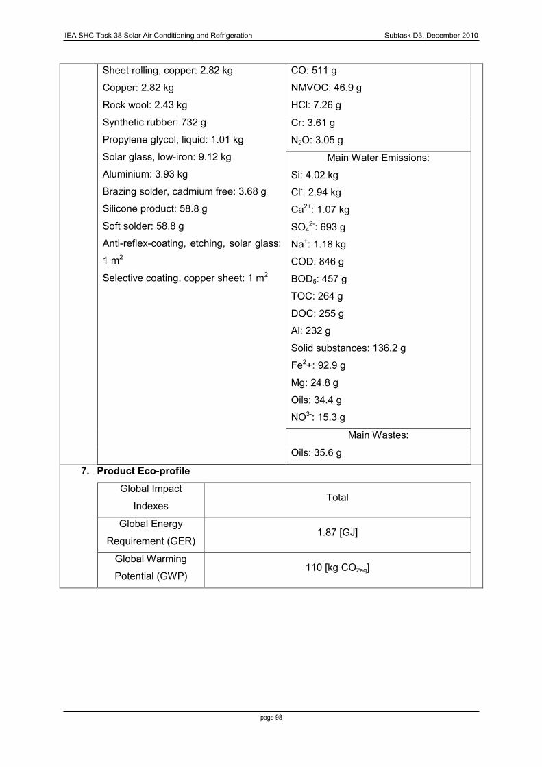
IEA SHC Task 38 Solar Air Conditioning and Refrigeration Subtask D3, December 2010
page 98
Sheet rolling, copper: 2.82 kg
Copper: 2.82 kg
Rock wool: 2.43 kg
Synthetic rubber: 732 g
Propylene glycol, liquid: 1.01 kg
Solar glass, low-iron: 9.12 kg
Aluminium: 3.93 kg
Brazing solder, cadmium free: 3.68 g
Silicone product: 58.8 g
Soft solder: 58.8 g
Anti-reflex-coating, etching, solar glass:
1 m2
Selective coating, copper sheet: 1 m2
CO: 511 g
NMVOC: 46.9 g
HCl: 7.26 g
Cr: 3.61 g
N2O: 3.05 g
Main Water Emissions:
Si: 4.02 kg
Cl-: 2.94 kg
Ca2+: 1.07 kg
SO42-: 693 g
Na+: 1.18 kg
COD: 846 g
BOD5: 457 g
TOC: 264 g
DOC: 255 g
Al: 232 g
Solid substances: 136.2 g
Fe2+: 92.9 g
Mg: 24.8 g
Oils: 34.4 g
NO3-: 15.3 g
Main Wastes:
Oils: 35.6 g
7. Product Eco-profile
Global Impact
Indexes Total
Global Energy
Requirement (GER) 1.87 [GJ]
Global Warming
Potential (GWP) 110 [kg CO2eq]
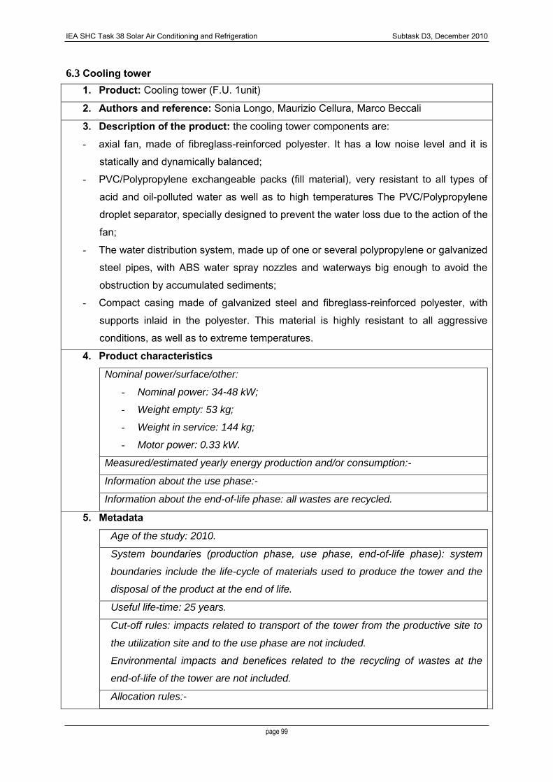
IEA SHC Task 38 Solar Air Conditioning and Refrigeration Subtask D3, December 2010
page 99
6.3 Cooling tower 1. Product: Cooling tower (F.U. 1unit)
2. Authors and reference: Sonia Longo, Maurizio Cellura, Marco Beccali
3. Description of the product: the cooling tower components are: - axial fan, made of fibreglass-reinforced polyester. It has a low noise level and it is
statically and dynamically balanced;
- PVC/Polypropylene exchangeable packs (fill material), very resistant to all types of
acid and oil-polluted water as well as to high temperatures The PVC/Polypropylene
droplet separator, specially designed to prevent the water loss due to the action of the
fan;
- The water distribution system, made up of one or several polypropylene or galvanized
steel pipes, with ABS water spray nozzles and waterways big enough to avoid the
obstruction by accumulated sediments;
- Compact casing made of galvanized steel and fibreglass-reinforced polyester, with
supports inlaid in the polyester. This material is highly resistant to all aggressive
conditions, as well as to extreme temperatures.
4. Product characteristics
Nominal power/surface/other:
- Nominal power: 34-48 kW;
- Weight empty: 53 kg;
- Weight in service: 144 kg;
- Motor power: 0.33 kW.
Measured/estimated yearly energy production and/or consumption:-
Information about the use phase:-
Information about the end-of-life phase: all wastes are recycled.
5. Metadata
Age of the study: 2010.
System boundaries (production phase, use phase, end-of-life phase): system
boundaries include the life-cycle of materials used to produce the tower and the
disposal of the product at the end of life.
Useful life-time: 25 years.
Cut-off rules: impacts related to transport of the tower from the productive site to
the utilization site and to the use phase are not included.
Environmental impacts and benefices related to the recycling of wastes at the
end-of-life of the tower are not included.
Allocation rules:-

IEA SHC Task 38 Solar Air Conditioning and Refrigeration Subtask D3, December 2010
page 100
Further details:-
Data Quality Assessment: estimation based to direct measurements.
6. Life Cycle Inventory
Main employed materials and
components:
Galvanized steel: 19.7 kg
Fibreglass-reinforced polyester: 19.4 kg
PVC: 11.5 kg
Polypropylene: 2.4 kg
Main Air Emissions:
CO2: 120.2 kg
CO: 593.3 g
CH4: 398.2 g
SO2: 331 g
NOx: 298 g
Particulates: 258 g
NMVOC: 125 g
N2O: 77 g
SO42-: 15.6 g
Al: 11.8 g
HCl: 6.62 g
CS2: 4.56 g
Main Water Emissions:
Cl-: 6.08 kg
Na+: 1.68 kg
Si: 1.58 kg
COD: 1.08 kg
BOD5: 514 g
SO42-: 479 g
Ca2+: 260 g
TOC: 191 g
DOC: 186 g
Solid substances: 77.4 g
Al: 66.5 g
Fe2+: 54.8 g
Mg: 25 g
Acetic acid: 24.2 g
K+: 21.1 g
Oils: 16.4 g
PO43-: 14.1 g
Main Wastes:
-
7. Product Eco-profile

IEA SHC Task 38 Solar Air Conditioning and Refrigeration Subtask D3, December 2010
page 101
Global Impact
Indexes Total
Global Energy
Requirement (GER) 2.97 [GJ]
Global Warming
Potential (GWP) 152.4 [kg CO2eq]

IEA SHC Task 38 Solar Air Conditioning and Refrigeration Subtask D3, December 2010
page 102
6.4 Dry cooling tower (Adsorption) 8. Product: dry cooling tower (F.U. 1unit)
9. Authors and reference: Lesbat (HEIG-VD, Switzerland)
10. Description of the product: The dry cooling tower (recooler) is the heat rejection
part of the installation.The major components are steel, aluminum, cooper and plastic
as PEHD.
11. Product characteristics
Nominal power/surface/other:
- Nominal power: 24 kW;
Measured/estimated yearly energy production and/or consumption:-
Information about the use phase:-
Information about the end-of-life phase: all metals are recycle and plastics are
burned
12. Metadata
Age of the study: 2010
System boundaries): production phase; All the components of the chiller are
included in the production phase. As we do not have the energy use for
fabrication phase, it is not included. No transport to the production site is taken in
account as we do not have those information. Use phase; during the use phase,
the energy is included in the LCIA of the whole installation. The maintenance is
negligible. The transport is not included. End-of-life phase; All components which
can be recycled have no impact (ecoinvent® rules) the rest is or for incineration,
or for disposal in CH. The recycling has a cut-off approach.
Useful life-time: 25 years.
Cut-off rules: impacts related to transport of the tower from the productive site to
the utilization site and to the use phase are not included.
The recycling has a cut-off approach.
Allocation rules:-
Further details:-
Data Quality Assessment: The amount of material results of the company data.
13. Life Cycle Inventory
Main employed materials and
components:
Steel : 86 kg
Aluminium : 58 kg
Cooper : 35 kg
Main Air Emissions:
Heat waste: 15136 MJ
CO2: 967.1 kg
SO2: 17.6 kg
CO: 8.8 kg

IEA SHC Task 38 Solar Air Conditioning and Refrigeration Subtask D3, December 2010
page 103
Plastic (PEHD) : 35 kg NOx: 6.5 kg
CH4: 2.1 kg
Particulates: 4.3 kg
Water: 1.2 kg
Al: 800 g
NMVOC: 702 g
CS2: 408 g
NH3: 327 g
Cu: 89 g
Pb: 80 g
Ni: 63 g
HF: 42 g
Main Water Emissions:
Heat waste: 803.3 MJ
Si: 23.7 kg
SO42-: 12.1 kg
Na+: 7.1 kg
Cl-: 6.1 kg
Ca2+: 4.7 kg
COD: 3.7 kg
Al: 2.6 kg
BOD5: 1.9 kg
TOC: 1.3 kg
DOC: 1.3 kg
Ti+: 997 g
Fe2+: 640 g
Solid substances: 406 g
Solved solids: 344 g
Oils: 333 g
F-: 250 g
PO43-: 14.1 g
Main Wastes:
Heat waste: 22.65 MJ
Oils: 345 g
14. Product Eco-profile
Global Impact
Indexes Total

IEA SHC Task 38 Solar Air Conditioning and Refrigeration Subtask D3, December 2010
page 104
Global Energy
Requirement (GER) 14.345[GJ]
Global Warming
Potential (GWP) 770 [kg CO2eq]

IEA SHC Task 38 Solar Air Conditioning and Refrigeration Subtask D3, December 2010
page 105
6.5 Heat pump brine-water 1. Product: Heat pump brine-water (F.U. 1 unit)
2. Authors and reference: data published by Thomas Heck in Ecoinvent ver.2.0
3. Description of the product: heat pump brine-water 10 kW of output. Refrigerant
R134a.
4. Characteristics of the product
Nominal power/surface/other: power 10 kW
Measured/estimated yearly energy production and/or consumption:-
Information about the use phase:-
Information about the end-of-life phase: plastic wastes are incinerated. The end-of-
life of other wastes is not included.
5. Metadata
Age of the study: 2004.
System boundaries (production phase, use phase, end-of-life phase): The module
includes the most important materials used for production. It includes also the
transport of these materials, energy and water needed for production. It includes
emissions of refrigerant (R134a) during production and scrapping. It does not
include emissions during operation. It does not include the borehole heat
exchanger. A buffer heat storage is not included. Data are referred to the end of
life of some parts of the product.
Useful life-time: 25 years.
Cut-off rules: impacts related to transport of the storage from the productive site to
the utilization site and to the use phase are not included.
Allocation rules:
Further details:
Data Quality Assessment: input data have been collected using literature and
manufacturer information.
6. Life Cycle Inventory
Main employed materials and
components:
Electricity, medium voltage: 140 kWh
Natural gas: 1400 MJ
Tube insulation, elastomere: 10 kg
Refrigerant R134a: 3.09 kg
Copper: 22 kg
Polyvinylchloride: 1 kg
Main Air Emissions:
CO2: 376.9 kg
CO: 2.52 kg
Particulates: 1.35 kg
CH4: 963.8 g
NOx: 1.07 kg
SO2: 3.17 kg
NMVOC: 263 g

IEA SHC Task 38 Solar Air Conditioning and Refrigeration Subtask D3, December 2010
page 106
Steel, low-alloyed: 20 kg
Reinforcing steel: 75 kg
Lubricating oil: 1.7 kg
Al: 188 g
NH3: 78.9 g
HCl: 13.9 g
Cr: 1,58 g
Si: 2.19 g
N2O: 10.6 g
Main Water Emissions:
Si: 5.61 kg
Cl-: 3.93 kg
SO42-: 2.77 kg
COD: 1.01 kg
Ca2+: 1.28 kg
BOD5: 479 g
TOC: 430 g
DOC: 428 g
Na+: 1.51 kg
Solid substances: 269 g
Fe2+: 190 g
Al: 184 g
Mg: 85.9 g
PO43-: 60.2 g
Oils: 75 g
K+: 42.7 g
Main Wastes:
Oils: 74.5
7. Product Eco-profile
Global Impact
Indexes Total
Global Energy
Requirement (GER) 8.18 [GJ]
Global Warming
Potential (GWP) 1590 [kg CO2eq]

IEA SHC Task 38 Solar Air Conditioning and Refrigeration Subtask D3, December 2010
page 107
6.6 Heat storage 8. Product: Heat storage (F.U. 1 unit)
9. Authors and reference: data published by Niels Jungbluth in Ecoinvent ver.2.0
10. Description of the product: heat storage with a capacity of 2000 l for use in a
solar collector heating system
11. Characteristics of the product
Nominal power/surface/other: capacity 2000 l
Measured/estimated yearly energy production and/or consumption:-
Information about the use phase:-
Information about the end-of-life phase: packaging wastes are incinerated. Rock
wool wastes are recovered. The end-of-life of other wastes is not included.
12. Metadata
Age of the study: 2003.
System boundaries (production phase, use phase, end-of-life phase): data are
referred to the production of an heat storage in Switzerland, including materials
and energy use of production, and disposal of the product at the end of life.
Useful life-time: 25 years.
Cut-off rules: impacts related to transport of the storage from the productive site to
the utilization site and to the use phase are not included.
Allocation rules:
Further details:
Data Quality Assessment: input data of materials used to produce the storage
have been collected using questionnaires.
Data have been validated.
13. Life Cycle Inventory
Main employed materials and
components:
Electricity, medium voltage: 45 kWh
Electricity, photovoltaic: 45 kWh
Natural gas: 198 MJ
Energy from biomass (wood): 146 MJ
Rock wool: 25 kg
Chromium steel: 35 kg
Steel: 305 kg
Water: 800 kg
Main Air Emissions:
CO2: 796 kg
CO: 8.11 kg
Particulates: 3.89 kg
CH4: 2.14 kg
NOx: 2.03 kg
SO2: 2 kg
NMVOC: 417 g
Al: 181 g
NH3: 140 g
HCl: 73.8 g

IEA SHC Task 38 Solar Air Conditioning and Refrigeration Subtask D3, December 2010
page 108
CS2: 69 g
Cr: 39,6 g
Si: 17.8 g
N2O: 16.3 g
Main Water Emissions:
Si: 44.3 kg
Cl-: 5.46 kg
SO42-: 4.1 kg
COD: 2.89 kg
Ca2+: 2.78 kg
BOD5: 1.27 kg
TOC: 1.1 kg
DOC: 1.1 kg
Na+: 1.03 kg
Solid substances: 1.2 kg
Fe2+: 794 g
Al: 678 g
Mg: 240 g
PO43-: 207 g
Oils: 137 g
K+: 118 g
Main Wastes:
Oils: 126
14. Product Eco-profile
Global Impact
Indexes Total
Global Energy
Requirement (GER) 15.2 [GJ]
Global Warming
Potential (GWP) 780.9 [kg CO2eq]

IEA SHC Task 38 Solar Air Conditioning and Refrigeration Subtask D3, December 2010
page 109
6.7 Gas boiler 1. Product: Gas boiler (F.U. 1 unit)
2. Authors and reference: data published by Thomas Heck in Ecoinvent ver.2.0
3. Description of the product Gas boiler (10 kW of power)
4. Characteristics of the product
Nominal power/surface/other: power 10 kW
Measured/estimated yearly energy production and/or consumption::
Information about the use phase:
Information about the end-of-life phase: wastes as plastics, packaging and
hazardous wastes are incinerated. Rock wool wastes are discharged in an inert
material landfill. The end-of-life of other wastes is not included.
5. Metadata
Age of the study: Materials data have been investigated in 1993. Data for
energy use during the production phase have been estimated on the basis of an
environmental report for 1998.
System boundaries (production phase, use phase, end-of-life phase): data are
referred to the production of a gas boiler in Switzerland and in Germany,
including materials and energy use of production, and disposal of the product at
the end of life. The transport of these materials and the energy and water
needed for production are included.
Useful life-time:25 years
Cut-off rules: impacts related to transport of the gas boiler from the productive
site to the utilization site and to the use phase are not included.
Allocation rules:
Further details:
Data Quality Assessment: input data have been extrapolated assuming that the
material requirement for a gas boiler is approximately the same as for an oil
boiler. Moreover, is has been assumed that these materials are about the same
in modern (2000) boilers as well as in average installed boilers.
6. Life Cycle Inventory
Main employed materials and
components:
Electricity, medium voltage: 81.7 kWh
Natural gas: 472 MJ
Light fuel oil: 249 MJ
Water: 182 kg
Main Air Emissions
SO2: 1.4 kg
CO2: 371.5 kg
CO: 3.19 kg
Particulates: 1.53 kg
CH4: 0.9 kg

IEA SHC Task 38 Solar Air Conditioning and Refrigeration Subtask D3, December 2010
page 110
Alkyd paint, white, 60% in solvent: 1.25
kg
Aluminium: 7.5 kg
Brass: 0.05 kg
Brazing solder, cadmium free: 4 kg
Chromium steel: 5 kg
Copper: 3.03 kg
Polyethylene, HDPE granulate: 0.9 kg
Rock wool: 8 kg
Corrugated board, mixed fibres: 5 kg
Steel, low-alloyed: 115 kg
NOx: 0.96 kg
NMVOC: 201 g
Al: 113 g
NH3: 57.9 g
HCl: 20.7 g
CS2: 50 g
N2O: 9.36 g
Main Water Emissions
Si: 12.4 kg
Cl-: 2.92 kg
SO42-: 2.46 kg
COD: 1.15 kg
Ca2+: 1.14 kg
BOD5: 598 g
TOC: 434 g
DOC: 430 g
Na+: 0.79 kg
Solid substances: 664 g
Fe2+: 247 g
Al: 266 g
Mg: 93.4 g
PO43-: 81.5 g
Oils: 93.2 g
K+: 41 g
Main Wastes:
Oils: 90.9 g
7. Product Eco-profile
Global Impact Indexes Total Per unit of power
Global Energy Requirement
(GER) 7 [GJ] 0.7 [GJ/kW]
Global Warming Potential (GWP) 392 [kg CO2eq] 39.2 [kg CO2eq/kW]