IEEETRANSACTIONS ON GEOSCIENCE AND REMOTE SENSING … · remote sensing images is of great interest for both civilian and ... sample) is therefore a ... neously link the target pixels

This article has been accepted for inclusion in a future issue of this journal. Content is final as presented, with the exception of pagination.

IEEE TRANSACTIONS ON GEOSCIENCE AND REMOTE SENSING 1

Hyperspectral Remote Sensing Image SubpixelTarget Detection Based on Supervised

Metric LearningLefei Zhang, Member, IEEE, Liangpei Zhang, Senior Member, IEEE, Dacheng Tao, Senior Member, IEEE,

Xin Huang, Member, IEEE, and Bo Du, Member, IEEE

Abstract—The detection and identification of target pixels suchas certain minerals and man-made objects from hyperspectralremote sensing images is of great interest for both civilian andmilitary applications. However, due to the restriction in the spatialresolution of most airborne or satellite hyperspectral sensors, thetargets often appear as subpixels in the hyperspectral image (HSI).The observed spectral feature of the desired target pixel (positivesample) is therefore a mixed signature of the reference targetspectrum and the background pixels spectra (negative samples),which belong to various land cover classes. In this paper, we pro-pose a novel supervised metric learning (SML) algorithm, whichcan effectively learn a distance metric for hyperspectral targetdetection, by which target pixels are easily detected in positivespace while the background pixels are pushed into negative spaceas far as possible. The proposed SML algorithm first maximizesthe distance between the positive and negative samples by anobjective function of the supervised distance maximization. Then,by considering the variety of the background spectral features, weput a similarity propagation constraint into the SML to simulta-neously link the target pixels with positive samples, as well as thebackground pixels with negative samples, which helps to rejectfalse alarms in the target detection. Finally, a manifold smoothnessregularization is imposed on the positive samples to preserve theirlocal geometry in the obtained metric. Based on the public datasets of mineral detection in an Airborne Visible/Infrared ImagingSpectrometer image and fabric and vehicle detection in a Hyper-spectral Mapper image, quantitative comparisons of several HSItarget detection methods, as well as some state-of-the-art metriclearning algorithms, were performed. All the experimental resultsdemonstrate the effectiveness of the proposed SML algorithm forhyperspectral target detection.

Index Terms—Dimension reduction, hyperspectral image (HSI),metric learning, target detection.

Manuscript received December 19, 2012; revised May 21, 2013 and August23, 2013; accepted October 10, 2013. This work was supported in part bythe National Basic Research Program of China (973 Program) under Grant2011CB707105 and Grant 2012CB719905; by the Program for ChangjiangScholars and Innovative Research Team in University (IRT1278); by theNational Natural Science Foundation of China under Grant 41101336, Grant61102128, and Grant 41061130553; and by the Program for New CenturyExcellent Talents in University of China under Grant NCET-11-0396.

L. Zhang and B. Du are with the Computer School, Wuhan University,Wuhan 430072, China (e-mail: [email protected]; [email protected]).

L. Zhang and X. Huang are with the State Key Laboratory of InformationEngineering in Surveying, Mapping, and Remote Sensing, Wuhan University,Wuhan 430079, China (e-mail: [email protected]; [email protected]).

D. Tao is with the Centre for Quantum Computation and Intelligent Systemsand the Faculty of Engineering and Information Technology, University ofTechnology, Sydney, Ultimo, NSW 2007, Australia (e-mail: [email protected]).

Color versions of one or more of the figures in this paper are available onlineat http://ieeexplore.ieee.org.

Digital Object Identifier 10.1109/TGRS.2013.2286195

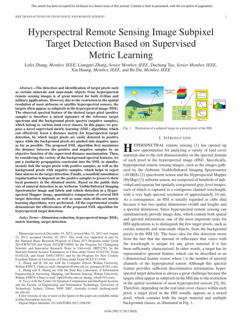
Fig. 1. Illustration of a subpixel target in a mixed pixel of the HSI.

I. INTRODUCTION

HYPERSPECTRAL remote sensing [1] has opened upnew opportunities for analyzing a variety of land cover

materials due to the rich dimensionality on the spectral domainof each pixel in the hyperspectral image (HSI). Specifically,hyperspectral remote sensing images, such as the images gath-ered by the Airborne Visible/Infrared Imaging Spectrometer(AVIRIS) [2] spaceborne sensor and the Hyperspectral Mapper(HyMap) [3] airborne sensor, are composed of hundreds of indi-vidual and separate but spatially coregistered gray-level images,each of which is captured in a contiguous channel wavelength,with a very high spectral resolution of approximately 10 nm.As a consequence, an HSI is usually regarded as cube databecause it has two spatial dimensions (width and height) anda spectral dimension. Since hyperspectral remote sensing cansimultaneously provide image data, which contain both spatialand spectral information, one of the most important tasks forHSI applications is to distinguish the few target pixels, such ascertain minerals and man-made objects, from the backgroundpixels in the HSI [4]. The basic idea for this detection stemsfrom the fact that the amount of reflectance that varies withthe wavelength is unique for any given material if it hasbeen sufficiently characterized. In other words, a target has itsrepresentative spectral feature, which can be described as anl-dimensional feature vector, where l is the number of spectralchannels of the hyperspectral sensor. Although this spectralfeature provides sufficient discriminative information, hyper-spectral target detection is always a great challenge because thetargets often appear as subpixels in the HSI due to the restrictionin the spatial resolution of most hyperspectral sensors [5], [6].Therefore, depending on the real land cover classes within eachpixel, a target pixel in the HSI usually appears as a mixedpixel, which contains both the target material and multiplebackground classes, as illustrated in Fig. 1.

0196-2892 © 2013 IEEE

mailto: [email protected]





2 IEEE TRANSACTIONS ON GEOSCIENCE AND REMOTE SENSING

To deal with mixed pixels in HSI analysis, it is widelyaccepted that the measured spectrum of a mixed pixel is afunction of the pure spectral features (end-members) of all thematerials in this pixel, with their weighting factors. The stan-dard technique is the linear mixture model (LMM) [7], whichsuggests that the measured spectrum is a linear combination ofthe end-members, weighted by their corresponding abundancefractions, which indicate the proportion of each end-memberpresent in the mixed pixel. The LMM is easy to implementand flexible in most conditions. However, as reviewed in [8],the nonlinear mixture model (NLMM) describes a mixed spec-trum by considering some more complex combinations of thecomponent reflectance spectra in the mixture, and often has aphysical meaning in that the radiation is reflected by multiplebounces in the hyperspectral imaging. For a more comprehen-sive explanation of the distinctions between the LMM and theNLMM for HSI spectral unmixing, refer to [9] and [10].

The existing HSI subpixel target detection algorithms inthe remote sensing area mainly focus on formulating specificobservation models for the target and background pixels [11].

1) Spectral-unmixing-based models (structured backgroundmodels), most of which are LMM based. These methodsadopt the LMM with various constraints to characterizethe targets and the interfering background, with the con-sideration of additional random Gaussian sensor noise inthe model [12]. The adaptive matched subspace detector(AMSD) is such an algorithm that models the target andbackground characteristics by the LMM and recognizesthe probable subpixel targets by a statistical hypothesistest [13]. It should be noted that the LMM has to beextended into the NLMM in some situations, such aswhen the source radiation is multiple reflected beforebeing collected at the sensor.

2) Statistical-based models (unstructured background mod-els), such as the adaptive matched filter (AMF) [14], [15]and the adaptive coherence/cosine estimator [16], [17].These models assume that the background samples havespecific distributions and maximize the target featureresponse while suppressing the response of the unknownbackground feature.

3) Hybrid subpixel target detection methods, which formu-late the background with both structured and unstruc-tured models. These methods take advantage of the twokinds of model and generally show better performances,particularly when dealing with weak targets in complexbackgrounds [18], [19].

However, as aforementioned, all these algorithms followcertain assumptions, and they can only work well in certainconditions, e.g., the AMSD is based on the LMM, and the AMFassumes that the target and background covariance matrices areidentical.

In recent years, machine learning algorithms have been intro-duced into HSI processing, and it has been suggested that theycan perform well in the applications of dimension reduction[20], [21], image segmentation [22], [23], and classification[24], [25]. There have been also some related works on HSItarget detection [26], e.g., kernel-based target detection meth-ods [27], [28] and sparse-representation-based target detection

methods [29], [30]. However, few studies have been devotedto a target detection method that is benefited by a distancemetric in the feature space of HSI, by which target pixels areeasily detected in positive space while background pixels arepushed into negative space as far as possible. In fact, based onthe key innovative idea of metric learning [31], many differentalgorithms have been proposed and have been demonstrated tobe effective in dealing with challenging applications in com-puter vision and pattern recognition, e.g., face recognition [32],handwritten digit recognition [33], image retrieval [34], objecttracking [35], and gene expression data classification [36]. Ac-cording to the particular challenges in the HSI target detectiontask, the following issues should be properly addressed whenusing metric learning for hyperspectral target detection: 1) asthe interested target pixels (positive samples) often appear assubpixels in the HSI, the observed target pixels spectra mightbe similar to the background pixels (negative samples) spectrain the original feature space; and 2) as the target pixels areoften very limited in number and the background pixels belongto various land cover classes, which include almost all thepixels in the HSI [37], the learned distance metric shouldremove as many background pixels as possible from the targetpixels.

In this paper, a novel supervised metric learning (SML)algorithm, which can effectively learn a distance metric forHSI target detection, is introduced in response to the afore-mentioned two aspects. As a machine-learning-based approach,no physically meaningful model is needed. By considering thespectral features of both negative samples (background pixels)and positive samples (mixed pixels with the target signature),the distance metric provided by SML results in the target pixelsbeing easily detected in positive space while the backgroundpixels are pushed into negative space as far as possible. Thus,the target detection measurement can be obtained by the spec-tral similarity between the test sample and the prior targetfeature using the learned distance metric. In particular, the SMLalgorithm first maximizes the distance between the positiveand negative samples by a supervised distance maximization.Then, by considering that the background pixels belong tovarious classes, a similarity propagation constraint is addedinto the SML to simultaneously link the target pixels withpositive samples, as well as the background pixels with negativesamples, which helps to reduce the false alarm rate. Finally, amanifold smoothness regularization of all the positive samplesis considered to preserve their local geometry in the obtainedmetric.

The rest of this paper is organized as follows. In Section II,we give a brief review of the metric learning algorithms. Wethen provide the detailed explanation of our SML algorithmfor HSI subpixel target detection in Section III. The HSItarget detection experimental results are reported in Section IV,followed by the conclusion in Section V.

II. RELATED WORKS

We assume that we have the following given data set X =[x1, . . . ,xn] ∈ Rl×n, in which n is the number of samples andl is the number of features, with the label information C =


ZHANG et al.: HYPERSPECTRAL REMOTE SENSING IMAGE SUBPIXEL TARGET DETECTION 3

[c1, . . . , cn]T , ci ∈ {+1,−1}. Thus, we have the following

similar constraints set Λ and dissimilar constraints set Ω:

Λ : ∀(xi,xj) |ci=cj ∈ Λ (1)

Ω : ∀(xi,xj) |ci �=cj ∈ Ω. (2)

The goal of metric learning is to learn a Mahalanobis-likedistance metric d(xi,xj), by which the distance between xi

and xj can be computed as

d(xi,xj) =√

(xi − xj)TM(xi − xj). (3)

To ensure that d(xi,xj) is a metric, the learnedMahalanobis-like matrix M ∈ Rl×l must be symmetricand positive semidefinite. Note that if M = I , then theMahalanobis-like distance is equal to the Euclidean distance. IfM is restricted to be diagonal, then the distance metric is equalto the Euclidean distance, but the different features are givendifferent weights. Furthermore, we can find a nonsquare matrixW ∈ Rl×d (d ≤ l) to jointly perform dimensionality reduction(DR) and metric learning [38], [39]

d(xi,xj) =√

(xi − xj)TM(xi − xj)

=

√(xi − xj)TWWT(xi − xj)

= ‖ WTxi −WTxj ‖ . (4)

Learning such a distance metric M as given in (4) is equiva-lent to finding a DR transformation of data that replaces eachpoint xi ∈ Rl with WTxi ∈ Rd and applying the standardEuclidean distance to the new data [31].

The various different distance metric learning methods usu-ally learn a specific matrix M (or W ) under the supervision ofconstraint sets Λ and Ω, such that the samples from differentclasses can be well discriminated. Xing et al. [31] formu-lated such a problem as a constrained convex programmingalgorithm, and the method introduced by Davis et al. [40]learns the Mahalanobis distance function from an information-theoretic perspective. Relevant component analysis (RCA) [41]uses adjustment learning to reduce irrelevant variability in thedata while amplifying relevant variability. Discriminative com-ponent analysis (DCA) [34] extends RCA by the exploitationof negative constraints and captures the nonlinear relationshipsbetween data instances with the contextual information. Largemargin nearest neighbor (LMNN) [33] trains the metric with thegoal that the k-nearest neighbors (KNNs) always belong to thesame class while examples from different classes are separatedby a large margin. Neighborhood component analysis (NCA)[32] learns the distance metric by maximizing a stochasticvariant of the leave-one-out KNNs score on the training set.

III. SML ALGORITHM FOR HSI TARGET DETECTION

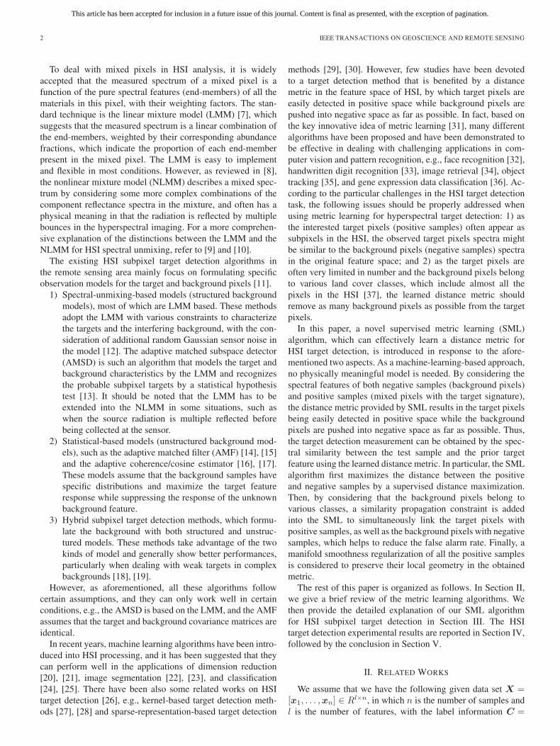
Fig. 2 shows the flowchart of the SML algorithm for HSItarget detection. The input items of SML include a set of pos-itive samples (red points) and negative samples (green points).The SML algorithm is then performed, the full optimization of

Fig. 2. Flowchart of the SML algorithm for HSI target detection.

which consists of the following three parts: 1) a supervised dis-tance maximization; 2) a similarity propagation constraint; and3) a manifold smoothness regularization. Detailed explanationsof these three parts are given in the following discussion. Sincethe SML learned distance metric is technically designed to bebeneficial for HSI target detection, the target detection task isthen simply achieved by sorting the samples that are nearestneighbors of the prior target feature, using the Mahalanobis-like distance metric in (4).

A. Supervised Distance Maximization

We follow the definitions given in the previous section inthat we have the observed data set X ∈ Rl×n with its label in-formation C ∈ Rn. Here, n is the number of training samples,and l is the number of spectral channels in the HSI. We furtherdenote n+ and n− as the number of positive and negative sam-ples, respectively; and thus, n = n+ + n−. Similar to [35] and[42], supervised distance maximization for target detection ismeasured by maximizing the average distance between positiveand negative samples while minimizing the average distancebetween positive samples in the learned distance metric. Byunifying the preceding two aspects together, we have

argmaxW

⎛⎜⎜⎜⎝

ci=+1∑i

cj=−1∑j

‖WTxi −WTxj ‖2

n+n−

−α

ci=+1∑i

cj=+1∑j

Qij‖WTxi −WTxj‖2

n+n+

⎞⎟⎟⎟⎠ (5)

in which α > 0 is a weighting factor used to control these twoparts; the matrix Q ∈ Rn×n in (5) is introduced from Laplacianeigenmaps [43] for locality preservation. Thus

Qij = exp(‖ xi − xj‖2/t) (6)

in which the radius parameter t can be experientially set to thesum of the variance of all the positive samples.



The supervised distance maximization in (5) finds a metricdistance that is the most discriminative for distinguishing targetpixels from background ones. However, it only tries to max-imize the average pairwise distances among the positive andnegative samples, and there are no restraints on the negativeand positive samples to deal with the variety of backgroundspectra and the local geometry of the target manifold space, re-spectively. We therefore further impose the following similaritypropagation constraint and manifold smoothness regularizationinto the SML.

B. Similarity Propagation Constraint

To enable the proposed SML to work well for HSI tar-get detection, we should give more restraint to each trainingsample to further shrink the distances between similar pairs.In this paper, a similarity propagation constraint is suggestedto simultaneously link the target pixels with positive samples,as well as the background pixels with negative samples. Thisconstraint aims to learn an optimal intrinsic similarity matrixS ∈ Rn×n, which measures the similarities between all thesample pairs by propagating a strong similarity (defined by thelabel information) to all the samples with a weak similarity. Acommon way to build the weak similarity of sample pairs is theKNN-graph-based pairwise connection, which is defined by theneighborhood indicator matrix G ∈ Rn×n, i.e.,

Gij =

{1, xj ∈ K(xi)0, otherwise

(7)

in which Gii| ni=1 = 0, and K(xi) denotes the sample set of the

KNNs of xi by the Euclidean metric in the whole set. Notethat such a matrix G holds weak (probably correct) similaritiesbetween all the sample pairs since it does not address anysupervised information from the training samples. To build astrong similarity matrix H ∈ Rn×n, we have

Hij =

{1, xj ∈ K(xi)|(xi,xj)∈Λ0, otherwise

(8)

in which K(xi)|(xi,xj)∈Λ finds the KNNs of xi, also by theEuclidean metric, but only in the similar constraints set Λ.Again, we have Hii| n

i=1 = 0 in (8).For the initialization of the expected matrix S, we simply

set S(0) = H and S(0)ii | n

i=1 = 1. We then regard the elements

where S(0)ij = 1 as original positive energies and try to propa-

gate these energies to the other 0 elements in S(0), followingthe paths built in the weak similarity matrix G. The criterion ofthis similarity propagation can be formulated as [44]

S(t+1)i = (1− γ)S

(0)i + γ

∑j

GijS(t)i∑

j

Gij(9)

where S(t)i denotes the ith row of matrix S at the tth iteration,

and γ is a parameter in the similarity propagation restricted by0 < γ < 1, which indicates the relative amount of the informa-

tion from its neighbors and its initial supervised information.The matrix form of (9) is written as

S(t+1) = (1− γ)S(0) + γPS(t) (10)

in which P = D−1G, as with the well-known transition prob-ability matrix in the Markov random walk models, and D is adiagonal matrix whose diagonal elements equal the sum of thecorresponding row elements in G, i.e., Dii =

∑j Gij .

Since 0 < γ < 1 and the eigenvalues of P are in [−1, 1],the sequence {S(t)} converges, and it suffices to solve the limitas [45]

S∗ = limt→∞

S(t) = (1− γ)(I − γP )−1S0. (11)

Thus, we can compute S∗ directly without iterations. It isworth noting that (I − γP )−1 is in fact a graph or a diffusionkernel [46]. Next, we can obtain the expected similarity matrixS by symmetrizing S∗ and removing the small similarityvalues, i.e.,

S =

(S∗ + S∗T

2

)≥ϕ

. (12)

In (12), we zero out the elements of S, whose absolute valuesare smaller than the threshold ϕ.

By the aforementioned similarity matrix S, we have thesimilarity propagation constraint

argminW

⎛⎜⎜⎝∑i

∑j

Sij

∥∥WTxi −WTxj

∥∥2n2

⎞⎟⎟⎠ . (13)

Subsequently, by adding (13) into (5) with a weighting factorβ > 0, we have

argmaxW

⎛⎜⎜⎜⎝

ci=+1∑i

cj=−1∑j

‖WTxi −WTxj‖2

n+n−

− α

ci=+1∑i

cj=+1∑j

Qij‖WTxi −WTxj‖2

n+n+

−β

∑i

∑j

Sij‖WTxi −WTxj‖2

n2

⎞⎟⎠ . (14)

In order to simplify the optimization (14), we build a unifiedmatrix T ∈ Rn×n with the same size as the similarity matrixS, each element of which encodes a pairwise weighting factorprovided in (14). Matrix T can be easily obtained by consider-ing separately for each part and then putting them together as awhole, i.e.,

T ij =

⎧⎨⎩

−βSij/n2 − αQij/n

+2, ci = cj = +1−βSij/n

2, ci = cj = −1−βSij/n

2 + 1/n+n−, cicj = −1.(15)



We then rewrite (14) as

argmaxW

⎛⎝∑

i

∑j

T ij‖WTxi −WTxj‖2⎞⎠

= argmaxW

tr[WTX(R− T )XTW

]

= argmaxW

tr(WTXLXTW

)

= argmaxW

tr(WTEW ) (16)

in which R is a diagonal matrix whose diagonal elements areequal to the sums of the corresponding row elements in T ,i.e., Rii =

∑j T ij , and L = R− T is known as the graph

Laplacian [43]. In order to further reduce (16), we denoteE = XLXT.

C. Manifold Smoothness Regularization

In the HSI subpixel target detection task, since the targetpixels are mixed with the background pixels from variousclasses, the input positive samples will be usually embeddedin a compact subspace, i.e., a low-dimensional manifold, con-sidering the spectral mixture, and thus, we expect the learnedmanifold of these positive samples to be as smooth as possible.In the proposed SML, the manifold smoothness of all thepositive samples is considered as an additional regularization topreserve their local geometry in the obtained metric [47], [48].The manifold smoothness can be quantitatively measured bythe reconstruction error of the famous locally linear embedding(LLE) algorithm [49]. In this work, we use a linear version ofLLE to build the minimization of the reconstruction error forthe positive samples. Following the aforementioned definitions,we denote the positive sample set as X+ = [x+

1 , . . . ,x+n+ ] ∈

Rl×n+. For each positive sample x+

i , the reconstruction erroris computed by the linear combination of the other samplesx+j |j �=i with weight Aij |j �=i, respectively. Thus

argminAij

∥∥∥∥∥∥x+i −

∑j �=i

Aijx+j

∥∥∥∥∥∥2

(17)

where A ∈ Rn+×n+, and Aii = 0. By the weight matrix given

above, we minimize the sum of the reconstruction errors of allthe positive samples in the measured space as

argminW

∑i

∥∥∥∥∥∥WTx+

i −∑j �=i

AijWTx+

j

∥∥∥∥∥∥2

. (18)

We can further rewrite (18) as follows:

argminW

tr[WTX+(I −AT)(I −AT)TX+TW

]

= argminW

tr[WTBW

](19)

where B = X+(I −AT)(I −AT)TX+T.Finally, by combining the supervised distance maximization

with the similarity propagation constraint introduced in (16)

and the manifold smoothness regularization provided in (19),we have the final optimization of SML, i.e.,

argminW

tr[WTEW − μ(WTBW )

]= argmin

Wtr[WT(E − μB)W

]= argmin

Wtr(WTZW ) (20)

in which μ is a weighting factor, and Z = E − μB. Equation(20) is famous in graph embedding methods [50], [51] and isoften enforced by a constraint in (21), which helps to removethe arbitrary scaling factor and uniquely determines W , i.e.,

argminW

tr(WTZW ) s.t. WWT = I. (21)

The solution of (21) is given by the top d eigenvectors associ-ated with the d smallest eigenvalues of the standard eigenvaluedecomposition

Zv = rv. (22)

IV. EXPERIMENTS

The experiments for HSI target detection are implemented ontwo public data sets.

1) An AVIRIS image, which covers the lunar crater volcanicfield (LCVF) in Northern Nye County, NV, USA. Thisdata set is public and is available at the National Aero-nautics and Space Administration website. Considered asa standard data set in HSI analysis, extensive researchwork has been undertaken in this area [52], [53]. Thefull spatial size of the LCVF data set is 6955 lines, with781 samples for each line. In our experiment, we usea subimage with a size of 400 × 400 pixels, the landcover types of which have been previously investigatedand comprise five main land cover classes, namely, redoxidized basaltic cinders, rhyolite, playa (dry lakebed),shade, and vegetation. We then implant the almandinespectrum into the image to simulate the subpixel targetsfor detection. The spatial resolution of the image is ap-proximately 20 m, and there are 224 spectral channelsfrom 0.4 to 2.5 μm.

2) A HyMap image, which was captured at the location ofthe small town of Cook City, MT, USA, on July 4, 2006.This image is a part of the Target Detection Test project[54] published by the Rochester Institute of Technology(RIT), Rochester, NY, USA, to serve as a standard dataset in HSI target detection. This data set project is alsoequipped with the exact locations and spectral library files(SPL) of all the desired targets. The full image size is 280×800 pixels, with 126 spectral channels in the visible-to-near infrared (VNIR)–short wave infrared (SWIR) range.The ground spatial resolution of the HSI is about 3 m, andthe spectral resolution is about 14 nm.

A. AVIRIS Experiment

The LCVF image scene used in our experiment is shown inFig. 3(a). In this HSI scene, we aim to detect the implanted



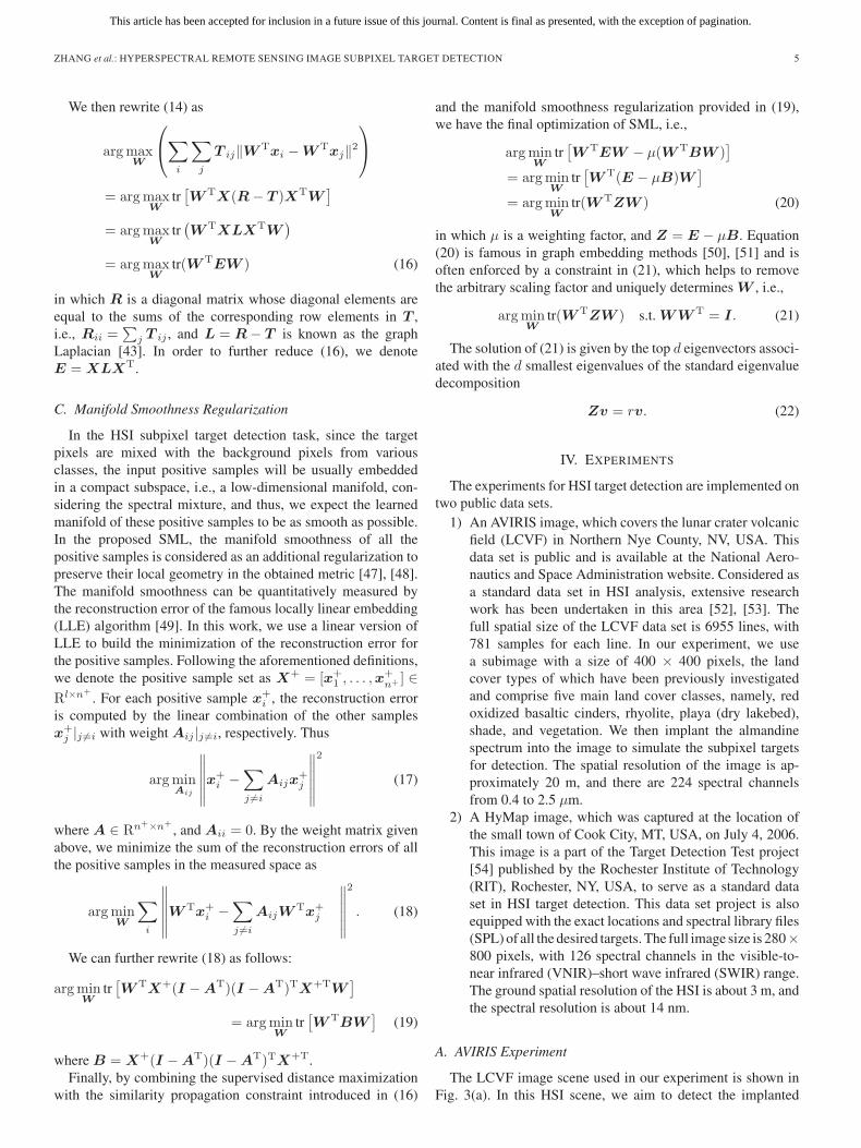
Fig. 3. (a) AVIRIS data cube of the LCVF. (b) Implanted target locations inthe AVIRIS image.

Fig. 4. (a) Implanted pure target spectrum and some representative back-ground samples spectra. (b) Locations of the background samples given in (a).

TABLE IDETAILS OF THE IMPLANTED TARGET PANELS IN FIG. 3

subpixel targets with different implanted fractions. The targetof interest is a mineral spectra named almandine, and weobtained its standard spectrum from the Environment for Visu-alizing Images spectral library (U.S. Geological Survey). Thespectral range of the pure target spectrum is from 0.39510 to2.56000 μm, with a spectral resolution of 0.002 μm. Therefore,in order to make it consistent with the AVIRIS data cube,we rescale the target spectra to the image range and resampleit according to the HSI wavelength. The adopted pure targetspectrum and some representative background spectral curvesare shown in Fig. 4(a), and the locations of the backgroundpixels are highlighted in Fig. 4(b). Then, in order to simulatea series of subpixels, to make the quantitative analysis possible,15 target panels are implanted into the image, the locations ofwhich are given in Fig. 3(b).

The added target panels have the same size, i.e., two pixelsfor each target panel, and the detailed coordinates of all 30implanted target pixels are given in Table I. Note that all theimplanted target pixels are mixed pixels, and each spectrumx is mixed with the prior target spectrum t and the original

background spectra b at the implanted locations, respectively,by both the LMM (23) and a representative NLMM (24), toevaluate the algorithms performance in subpixel target detec-tion. Thus

x = pt+ (1− p)b (23)

x =

√pt2 + (1− p)b2 (24)

in which the implanted fraction p varies from 10% to 2%, asindicated in Table I.

1) Linear Implanted Target Detection Results: We nowevaluate the subpixel target detection performance of the pro-posed algorithm. The SML algorithm requires training samplesto learn the distance metric; however, in the general hyper-spectral target detection task, only the pure target spectrum isavailable as prior information. Thus, in this paper, we proposeto generate the training samples for SML as follows: 1) forthe negative samples, we randomly select a certain number ofpixels from the HSI to represent the different background landcover classes, and we then set the number of negative samplesas [10, 20, 30, 40, 50] to explore its effect on the detectionaccuracy; and 2) for the positive samples, we mix the aforemen-tioned negative samples with the prior target spectrum, linearlyor nonlinearly, by a fixed fraction of p = 0.1, to simulate thevarious subpixel targets as the positive samples for the SMLalgorithm. Hence, the number of positive samples is equal to thenumber of negative samples in our experiments. Note that thereare five parameters in the SML algorithm, which we shouldpredefine as inputs. To address this issue, we propose to specif-ically determine their values as follows: We experimentallyset parameter α to 1 in the supervised distance maximizationterm and set parameter γ to 0.9 in the similarity propagationconstraint. The radius parameter t is set to the sum of thevariance of all the positive samples, as aforementioned. Theregularization parameters β and μ are data dependent, and thus,we have to optimize them by twofold cross-validation on thetraining samples. Empirically, these two parameters are usuallychosen as very small values for SML; in our experiments, theyare tuned by the range of β, μ ∈ 10[−6,−5,...,−2].

For the linear implanted targets, Fig. 5(a)–(e) shows thereceiver operating characteristic (ROC) [55] curves of the pro-posed algorithm with an increasing number of negative samplesfrom 10 to 50. It is clear that, when the number of negative sam-ples is low, the target detection performance is poor, because theSML algorithm requires more negative samples, which can rep-resent the various background land cover classes in HSI to learna better distance metric for discrimination. As a result, the ROCcurves improve as the number of negative samples increases, asshown in Fig. 5(b) and (c). When the number of negative sam-ples is increased to a larger value, the target detection resultsachieve a stable performance. Fig. 5(a)–(e) also empiricallyshow the effect of the similarity propagation constraint (13) andthe manifold smoothness regularization (19). In these figures,the solid lines indicate the ROC curves of the proposed SML,whereas the dashed lines give the performance of the distancemetric learned by supervised distance maximization (SDM),i.e., the optimization suggested in (5). It is shown that the



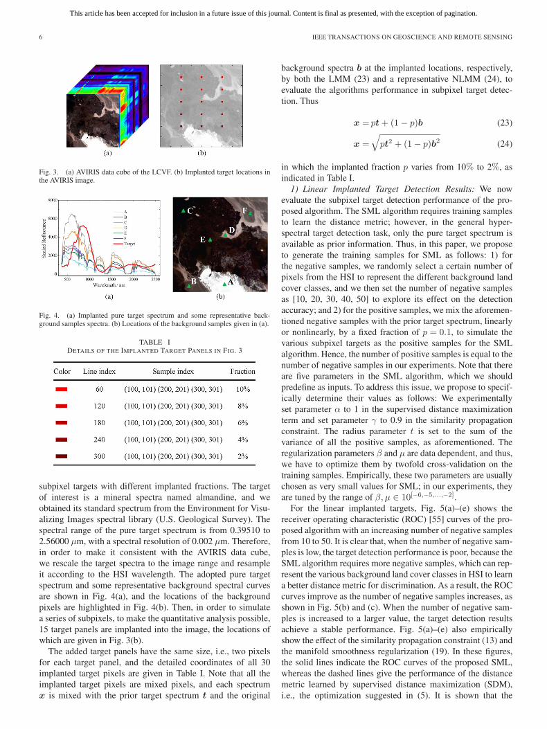
Fig. 5. (a)–(e) ROC curves of the SML and SDM algorithms with increasing numbers of negative samples (from 10 to 50).

Fig. 6. Three-dimensional target detection test statistic plots and 1-D transectplots of (a) AMF, (b) CEM, (c) DCA, (d) LMNN, (e) NCA, and (f) SML in thelinear implanted target experiment.

proposed SML outperforms SDM in all the ROC curves, whichconfirms the effectiveness of the recommended regularizations.

We then show the target detection results of the proposedSML compared with some of the other state-of-the-art tech-nologies on the AVIRIS data set, also for the linear implantedtargets. The AMF [17], constrained energy minimization(CEM) [52], DCA [34], LMNN [33], and NCA [32] algorithmsare applied as the comparisons in the experiment. Among thesealgorithms, AMF and CEM are effective HSI subpixel targetdetection algorithms that only need the desired target spectrumas input, whereas DCA, LMNN, and NCA are also distancemetric learning algorithms that require a set of training samples.Thus, we adopt the same training samples as SML, with thenumber of negative samples being 30, to learn the Mahalanobis-like distance metric for these four metric learning approaches.

Fig. 6(a)–(f) show the 3-D target detection test statistic plotsof all the aforementioned algorithms. For AMF and CEM, wedirectly show the algorithm output value as the test statisticfor each pixel in Fig. 6(a) and (b), whereas for the latterfour distance metric learning algorithms, the target detectionresults are measured by the distance of each pixel spectrum tothe prior target spectrum using the learned Mahalanobis-likedistance metric. In order to unify the presentation, we show thereciprocal of the distance as the test statistic in Fig. 6(c)–(f).Thus, as shown in Fig. 6, the higher test statistic indicates ahigher level of probability that the desired target presents at acertain pixel and vice versa. From these test statistic plots, we

can see that the target locations are obvious in the top threelines of the target panels (implanted fractions are no less than6%) for all the algorithms; however, when the abundance ofthe target in a mixed pixel is less than 6%, e.g., the bottomtwo lines of the target panels, which can be hardly observedin most of the algorithms, the separability between the targetand the background pixels is weak. Among these figures, theproposed SML suppresses the background pixels to a slightlylower range, and the target pixels can be easily recognized. Itshould be emphasized that, although the AMF algorithm cansuppress the background pixels to an even lower value, some ofthe target pixels are not clear enough, and the last line of thetarget panels (2% implanted fraction), in particular, is totallymissed in the detection.

To make the aforementioned target–background separabilityanalysis even clearer, we also show the 1-D transect plots of allthe algorithms in Fig. 6(a)–(f). These plots are the transects ofsample 200 in the 3-D target detection test statistic plots of allthe algorithms, respectively, each of which has five implantedtarget pixels at the line indices of 60, 120, 180, 240, and 300.As aforementioned, a higher test statistic value indicates ahigher level of probability that the desired target presents at acertain pixel. These 1-D transect plots further illustrate that onlyAMF, CEM, and the proposed SML algorithms can suppress thebackground pixels to a low and steady range; furthermore, theexpected peak in the transect plot of the target pixel at line 300(2% implanted fraction) can be hardly seen in Fig. 6(a), but canbe observed in Fig. 6(f), which suggests that SML can revealbetter separability between the target and background pixels.

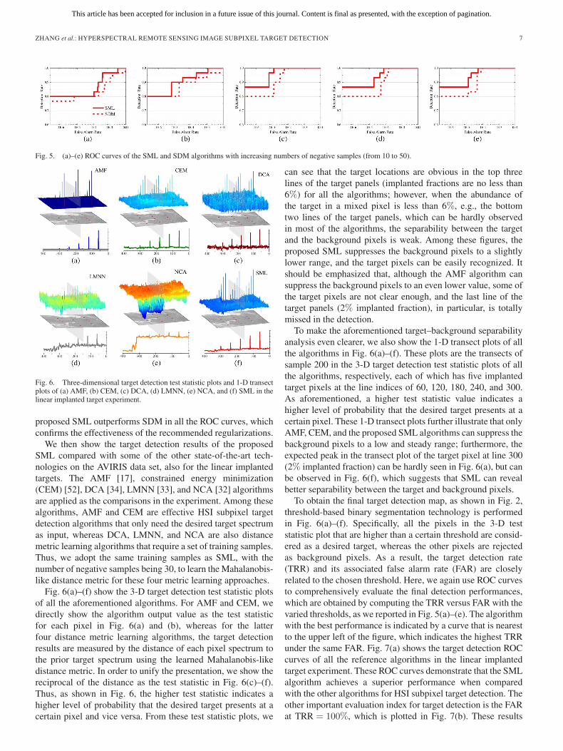
To obtain the final target detection map, as shown in Fig. 2,threshold-based binary segmentation technology is performedin Fig. 6(a)–(f). Specifically, all the pixels in the 3-D teststatistic plot that are higher than a certain threshold are consid-ered as a desired target, whereas the other pixels are rejectedas background pixels. As a result, the target detection rate(TRR) and its associated false alarm rate (FAR) are closelyrelated to the chosen threshold. Here, we again use ROC curvesto comprehensively evaluate the final detection performances,which are obtained by computing the TRR versus FAR with thevaried thresholds, as we reported in Fig. 5(a)–(e). The algorithmwith the best performance is indicated by a curve that is nearestto the upper left of the figure, which indicates the highest TRRunder the same FAR. Fig. 7(a) shows the target detection ROCcurves of all the reference algorithms in the linear implantedtarget experiment. These ROC curves demonstrate that the SMLalgorithm achieves a superior performance when comparedwith the other algorithms for HSI subpixel target detection. Theother important evaluation index for target detection is the FARat TRR = 100%, which is plotted in Fig. 7(b). These results



Fig. 7. (a) ROC curves and (b) FAR under 100% detection in the linearimplanted target experiment.

Fig. 8. Three-dimensional target detection test statistic plots and 1-D transectplots of (a) AMF, (b) CEM, (c) DCA, (d) LMNN, (e) NCA, and (f) SML in thenonlinear implanted target experiment.

Fig. 9. (a) ROC curves and (b) FAR under 100% detection in the nonlinearimplanted target experiment.

also suggest that the proposed SML algorithm results in thelowest FAR when all the target pixels have been recognized.

2) Nonlinear Implanted Target Detection Results: The HSItarget recognition results in the nonlinear implanted targetexperiment are similar to the linear condition. The 3-D targetdetection test statistic plots and the 1-D target detection teststatistic transect plots of sample 200 are shown in Fig. 8(a)–(f),respectively. These test statistic plots indicate the outstandingtarget–background separability of the proposed SML whencompared with the other methods. Based on the test statisticplots in Fig. 8(a)–(f), the target detection ROC curves of all thealgorithms are shown in Fig. 9(a), in which the curve of SMLis clearly in the upper-left location in the figure. In this curve,

Fig. 10. HyMap data cube of the RIT project.

the FAR is reduced to the 10-4 level when the TRR is at 90%.According to the experimental results reported here, both thelinear and nonlinear implanted target experiments suggest thatthe proposed SML is an effective approach for HSI subpixeltarget detection.

B. HyMap Experiment

Fig. 10 shows the HyMap data cube of the RIT project. In thisdata project, since both the radiance and the scaled reflectanceversion of the HSI are available, we use the scaled reflectanceimage and rescale the whole image by a reflectance factor of10 000 to the standard reflectance image. This HSI scene isairborne data, and the sensor was flown at approximately 1.4 kmabove the terrain, yielding a 3-m ground spatial resolution. Thus,the main background land cover classes can be manually inter-preted, and comprise roof, road, soil, grass, tree, and shadow,as shown in Fig. 10.

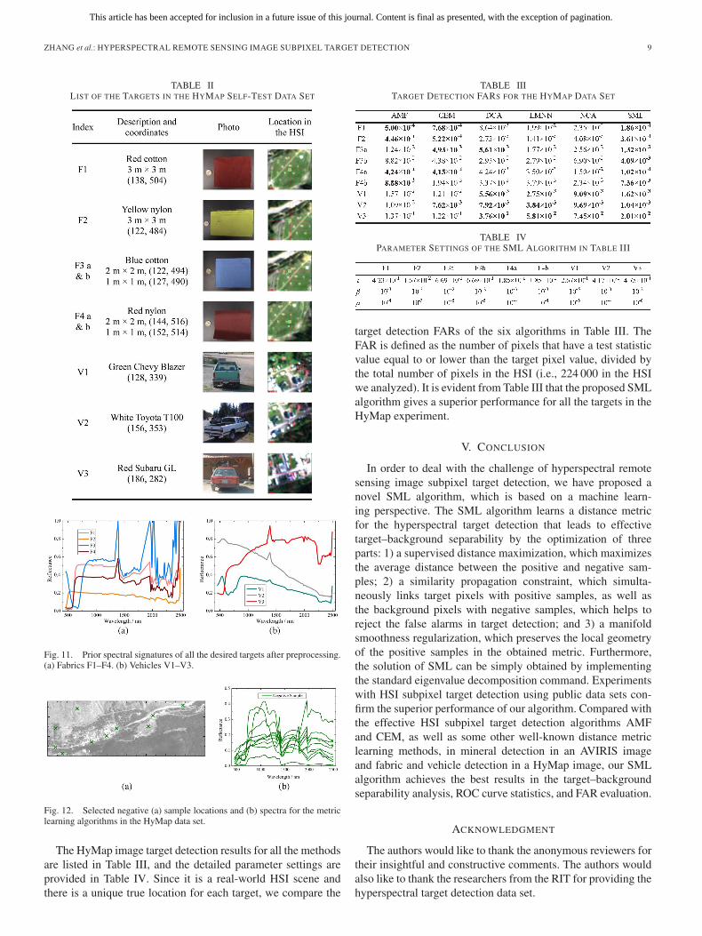
In this hyperspectral target detection image, several fabricpanels and vehicles of various sizes are deployed as targets.Details of these targets are listed in Table II. As the projectprovides the target size, we can infer that fabrics F1 and F2(3 m × 3 m) are nearly a full pixel, whereas all the otherfabric targets are smaller than a pixel and therefore occupysubpixels in the HyMap image. As regards the three vehicletargets, they occupy, at most, one or two pixels, which willalso appear as subpixels in the HSI, as shown in Table II. Insummary, all the subpixel targets in the HSI are visually difficultto recognize, and the only information we can use comes fromthe discriminative information brought about by the spectralsignature.

The prior spectrum of each target is obtained and prepro-cessed by the project-equipped SPL files. The SPL spectra werecollected in the field using an Analytical Spectral Device, i.e.,a FieldSpec Pro field spectrometer (note that the SPL were notmeasured in the air by the HyMap sensor), which can measurethe reflectance spectra from 350 to 2500 nm, with approxi-mately 1-nm spectral resolution. Then, by rescaling the SPLspectra to the true reflectance data (according to its reflectancefactor of 100) and resampling the SPL spectra according tothe HSI wavelength, we obtain the prior target spectra for theHSI target detection, as given in Fig. 11(a) and (b). For thedistance metric learning algorithms, we manually select tennegative samples that represent the different background landcover classes in the HyMap image. The negative samples areshown in Fig. 12(a), and their spectral curves are shown inFig. 12(b). We then generate the positive samples by the sameapproach used for the AVIRIS data set.



TABLE IILIST OF THE TARGETS IN THE HYMAP SELF-TEST DATA SET

Fig. 11. Prior spectral signatures of all the desired targets after preprocessing.(a) Fabrics F1–F4. (b) Vehicles V1–V3.

Fig. 12. Selected negative (a) sample locations and (b) spectra for the metriclearning algorithms in the HyMap data set.

The HyMap image target detection results for all the methodsare listed in Table III, and the detailed parameter settings areprovided in Table IV. Since it is a real-world HSI scene andthere is a unique true location for each target, we compare the

TABLE IIITARGET DETECTION FARS FOR THE HYMAP DATA SET

TABLE IVPARAMETER SETTINGS OF THE SML ALGORITHM IN TABLE III

target detection FARs of the six algorithms in Table III. TheFAR is defined as the number of pixels that have a test statisticvalue equal to or lower than the target pixel value, divided bythe total number of pixels in the HSI (i.e., 224 000 in the HSIwe analyzed). It is evident from Table III that the proposed SMLalgorithm gives a superior performance for all the targets in theHyMap experiment.

V. CONCLUSION

In order to deal with the challenge of hyperspectral remotesensing image subpixel target detection, we have proposed anovel SML algorithm, which is based on a machine learn-ing perspective. The SML algorithm learns a distance metricfor the hyperspectral target detection that leads to effectivetarget–background separability by the optimization of threeparts: 1) a supervised distance maximization, which maximizesthe average distance between the positive and negative sam-ples; 2) a similarity propagation constraint, which simulta-neously links target pixels with positive samples, as well asthe background pixels with negative samples, which helps toreject the false alarms in target detection; and 3) a manifoldsmoothness regularization, which preserves the local geometryof the positive samples in the obtained metric. Furthermore,the solution of SML can be simply obtained by implementingthe standard eigenvalue decomposition command. Experimentswith HSI subpixel target detection using public data sets con-firm the superior performance of our algorithm. Compared withthe effective HSI subpixel target detection algorithms AMFand CEM, as well as some other well-known distance metriclearning methods, in mineral detection in an AVIRIS imageand fabric and vehicle detection in a HyMap image, our SMLalgorithm achieves the best results in the target–backgroundseparability analysis, ROC curve statistics, and FAR evaluation.

ACKNOWLEDGMENT

The authors would like to thank the anonymous reviewers fortheir insightful and constructive comments. The authors wouldalso like to thank the researchers from the RIT for providing thehyperspectral target detection data set.



REFERENCES

[1] A. F. H. Goetz, G. Vane, J. E. Solomon, and B. N. Rock, “Imaging spec-trometry for Earth remote sensing,” Science, vol. 228, no. 4704, pp. 1147–1153, Jun. 1985.

[2] R. O. Green, M. L. Eastwood, C. M. Sarture, T. G. Chrien, M. Aronsson,B. J. Chippendale, J. A. Faust, B. E. Pavri, C. J. Chovit, M. Solis,M. R. Olah, and O. Williams, “Imaging spectroscopy and the AirborneVisible/Infrared Imaging Spectrometer (AVIRIS),” Remote Sens. Envi-ron., vol. 65, no. 3, pp. 227–248, Sep. 1998.

[3] T. Cocks, R. Jenssen, A. Stewart, I. Wilson, and T. Shields, “TheHyMapTM airborne hyperspectral sensor: The system, calibration andperformance,” in Proc. EARSEL Workshop Imag. Spectrosc., 1998,pp. 37–42.

[4] D. Manolakis, D. Marden, and G. A. Shaw, “Hyperspectral image process-ing for automatic target detection applications,” Lincoln Lab. J., vol. 14,no. 1, pp. 79–116, Jan. 2003.

[5] J. P. Kerekes and J. E. Baum, “Spectral imaging system analytical modelfor subpixel object detection,” IEEE Trans. Geosci. Remote Sens., vol. 40,no. 5, pp. 1088–1101, May 2002.

[6] B. Du and L. Zhang, “Random-selection-based anomaly detector for hy-perspectral imagery,” IEEE Trans. Geosci. Remote Sens., vol. 49, no. 5,pp. 1578–1589, May 2011.

[7] J. J. Settle and N. A. Drake, “Linear mixing and the estimation of groundcover proportions,” Int. J. Remote Sens., vol. 14, no. 6, pp. 1159–1177,1993.

[8] A. Plaza, Q. Du, J. M. Bioucas-Dias, X. Jia, and F. A. Kruse, “Forewordto the special issue on spectral unmixing of remotely sensed data,” IEEETrans. Geosci. Remote Sens., vol. 49, no. 11, pp. 4103–4110, Nov. 2011.

[9] N. Keshava and J. F. Mustard, “Spectral unmixing,” IEEE Signal Process.Mag., vol. 19, no. 1, pp. 44–57, Jan. 2002.

[10] J. M. Bioucas-Dias, A. Plaza, N. Dobigeon, M. Parente, Q. Du, P. Gader,and J. Chanussot, “Hyperspectral unmixing overview: Geometrical, statis-tical, and sparse regression-based approaches,” IEEE J. Sel. Topics Appl.Earth Observ. Remote Sens., vol. 5, no. 2, pp. 354–379, Apr. 2012.

[11] S. Matteoli, N. Acito, M. Diani, and G. Corsini, “An automatic approachto adaptive local background estimation and suppression in hyperspec-tral target detection,” IEEE Trans. Geosci. Remote Sens., vol. 49, no. 2,pp. 790–800, Feb. 2011.

[12] D. Manolakis, C. Siracusa, and G. Shaw, “Hyperspectral subpixel targetdetection using the linear mixing model,” IEEE Trans. Geosci. RemoteSens., vol. 39, no. 7, pp. 1392–1409, Jul. 2001.

[13] Q. Du and C.-I. Chang, “A signal-decomposed and interference-annihilated approach to hyperspectral target detection,” IEEE Trans.Geosci. Remote Sens., vol. 42, no. 4, pp. 892–906, Apr. 2004.

[14] I. S. Reed, J. D. Mallett, and L. E. Brennan, “Rapid convergence rate inadaptive arrays,” IEEE Trans. Aerosp. Electron. Syst., vol. AES-10, no. 6,pp. 853–863, Nov. 1974.

[15] F. C. Robey, D. R. Fuhrmann, E. J. Kelly, and R. Nitzberg, “A CFARadaptive matched filter detector,” IEEE Trans. Aerosp. Electron. Syst.,vol. 28, no. 1, pp. 208–216, Jan. 1992.

[16] S. Kraut and L. L. Scharf, “The CFAR adaptive subspace detector isa scale-invariant GLRT,” IEEE Trans. Signal Process., vol. 47, no. 9,pp. 2538–2541, Sep. 1999.

[17] S. Kraut, L. L. Scharf, and L. T. McWhorter, “Adaptive subspace detec-tors,” IEEE Trans. Signal Process., vol. 49, no. 1, pp. 1–16, Jan. 2001.

[18] L. Zhang, B. Du, and Y. Zhong, “Hybrid detectors based on selective end-members,” IEEE Trans. Geosci. Remote Sens., vol. 48, no. 6, pp. 2633–2646, Jun. 2010.

[19] J. Broadwater and R. Chellappa, “Hybrid detectors for subpixel targets,”IEEE Trans. Pattern Anal. Mach. Intell., vol. 29, no. 11, pp. 1891–1903,Nov. 2007.

[20] L. Zhang, L. Zhang, D. Tao, and X. Huang, “On combining multiple fea-tures for hyperspectral remote sensing image classification,” IEEE Trans.Geosci. Remote Sens., vol. 50, no. 3, pp. 879–893, Mar. 2012.

[21] W. Li, S. Prasad, J. E. Fowler, and L. M. Bruce, “Locality-preservingdimensionality reduction and classification for hyperspectral image anal-ysis,” IEEE Trans. Geosci. Remote Sens., vol. 50, no. 4, pp. 1185–1198,Apr. 2012.

[22] J. Li, J. M. Bioucas-Dias, and A. Plaza, “Semisupervised hyperspectralimage segmentation using multinomial logistic regression with activelearning,” IEEE Trans. Geosci. Remote Sens., vol. 48, no. 11, pp. 4085–4098, Nov. 2010.

[23] G. Bilgin, S. Ertrk, and T. Yldrm, “Segmentation of hyperspectral imagesvia subtractive clustering and cluster validation using one-class supportvector machines,” IEEE Trans. Geosci. Remote Sens., vol. 49, no. 8,pp. 2936–2944, Aug. 2011.

[24] M. Fauvel, J. A. Benediktsson, J. Chanussot, and J. R. Sveinsson, “Spec-tral and spatial classification of hyperspectral data using SVMs and mor-phological profiles,” IEEE Trans. Geosci. Remote Sens., vol. 46, no. 11,pp. 3804–3814, Nov. 2008.

[25] L. Bruzzone, M. Chi, and M. Marconcini, “A novel transductive SVMfor semisupervised classification of remote-sensing images,” IEEE Trans.Geosci. Remote Sens., vol. 44, no. 11, pp. 3363–3373, Nov. 2006.

[26] L. Zhang, L. Zhang, D. Tao, and X. Huang, “Sparse transfer man-ifold embedding for hyperspectral target detection,” IEEE Trans.Geosci. Remote Sens., vol. 52, no. 3, Mar. 2014. [Online]. Available:http://ieeexplore.ieee.org

[27] H. Kwon and N. M. Nasrabadi, “Kernel spectral matched filter for hy-perspectral imagery,” Int. J. Comput. Vis., vol. 71, no. 2, pp. 127–141,Feb. 2007.

[28] L. Capobianco, A. Garzelli, and G. Camps-Valls, “Target detection withsemisupervised kernel orthogonal subspace projection,” IEEE Trans.Geosci. Remote Sens., vol. 47, no. 11, pp. 3822–3833, Nov. 2009.

[29] Y. Chen, N. M. Nasrabadi, and T. D. Tran, “Simultaneous joint sparsitymodel for target detection in hyperspectral imagery,” IEEE Geosci. Re-mote Sens. Lett., vol. 8, no. 4, pp. 676–680, Jul. 2011.

[30] Y. Chen, N. M. Nasrabadi, and T. D. Tran, “Sparse representation for tar-get detection in hyperspectral imagery,” IEEE J. Sel. Top. Signal Process.,vol. 5, no. 3, pp. 629–640, Jun. 2011.

[31] E. P. Xing, A. Y. Ng, M.I. Jordan, and S. Russell, “Distance metriclearning, with application to clustering with side-information,” in Proc.NIPS, 2002, pp. 505–512.

[32] J. Goldberger, S. Roweis, G. Hinton, and R. Salakhutdinov, “Neighbour-hood components analysis,” in Proc. NIPS, 2004, pp. 513–520.

[33] K. Q. Weinberger and L. K. Saul, “Distance metric learning for largemargin nearest neighbor classification,” J. Mach. Learn. Res., vol. 10,pp. 207–244, Jun. 2009.

[34] S. C. H. Hoi, W. Liu, M. R. Lyu, and W.-Y. Ma, “Learning distance metricswith contextual constraints for image retrieval,” in Proc. CVPR, 2006,pp. 2072–2078.

[35] Z. Hong, X. Mei, and D. Tao, “Dual-force metric learning for robustdistracter-resistant tracker,” in Proc. ECCV , 2012, pp. 513–527.

[36] C.-C. Chang, “A boosting approach for supervised Mahalanobis distancemetric learning,” Pattern Recog., vol. 45, no. 2, pp. 844–862, Feb. 2012.

[37] D. Manolakis and G. Shaw, “Detection algorithms for hyperspectral imag-ing applications,” IEEE Signal Process. Mag., vol. 19, no. 1, pp. 29–43,Jan. 2002.

[38] F. Wang, “Semisupervised metric learning by maximizing constraint mar-gin,” IEEE Trans. Syst. Man Cybern. Part B, Cybern., vol. 41, no. 4,pp. 931–939, Aug. 2011.

[39] J. Yu, M. Wang, and D. Tao, “Semi-supervised multiview distance metriclearning for cartoon synthesis,” IEEE Trans. Image Process., vol. 21,no. 11, pp. 4636–4648, Nov. 2012.

[40] J. V. Davis, B. Kulis, P. Jain, S. Sra, and I. S. Dhillon, “Information-theoretic metric learning,” in Proc. ICML, 2007, pp. 209–216.

[41] N. Shental, T. Hertz, D. Weinshall, and M. Pavel, “Adjustment learningand relevant component analysis,” in Proc. ECCV , 2002, pp. 776–790.

[42] D. Tao, X. Tang, X. Li, and Y. Rui, “Direct kernel biased discriminantanalysis: A new content-based image retrieval relevance feedback algo-rithm,” IEEE Trans. Multimedia, vol. 8, no. 4, pp. 716–727, Aug. 2006.

[43] M. Belkin and P. Niyogi, “Laplacian eigenmaps for dimensionality reduc-tion and data representation,” Neural Comput., vol. 15, no. 6, pp. 1373–1396, Mar. 2003.

[44] W. Liu, X. Tian, D. Tao, and J. Liu, “Constrained metric learning viadistance gap maximization,” in Proc. AAAI, 2010, pp. 518–524.

[45] D. Zhou, O. Bousquet, T. N. Lal, J. Weston, and B. Scholkopf, “Learningwith local and global consistency,” in Proc. NIPS, 2004, pp. 321–328.

[46] J. Kandola, J. Shawe-Taylor, and N. Cristianini, “Learning semantic sim-ilarity,” in Proc. NIPS, 2002, pp. 657–664.

[47] T. Zhou and D. Tao, “Double shrinking for sparse dimension reduction,”IEEE Trans. Image Process., vol. 22, no. 1, pp. 244–257, Jan. 2013.

[48] W. Liu and D. Tao, “Multiview Hessian regularization for image annota-tion,” IEEE Trans. Image Process., vol. 22, no. 7, pp. 2676–2687, Jul. 2013.

[49] S. T. Roweis and L. K. Saul, “Nonlinear dimensionality reduction bylocally linear embedding,” Science, vol. 290, no. 22, pp. 2323–2326,Dec. 2000.

[50] S. Yan, D. Xu, B. Zhang, H.-J. Zhang, Q. Yang, and S. Lin, “Graph em-bedding and extensions: A general framework for dimensionality reduc-tion,” IEEE Trans. Pattern Anal. Mach. Intell., vol. 29, no. 1, pp. 40–51,Jan. 2007.

[51] T. Zhang, D. Tao, X. Li, and J. Yang, “Patch alignment for dimensionalityreduction,” IEEE Trans. Knowl. Data Eng., vol. 21, no. 9, pp. 1299–1313,Sep. 2009.

http://ieeexplore.ieee.org



[52] C.-I. Chang and D. C. Heinz, “Constrained subpixel target detection forremotely sensed imagery,” IEEE Trans. Geosci. Remote Sens., vol. 38,no. 3, pp. 1144–1159, Aug. 2000.

[53] J. C. Harsanyi and C.-I. Chang, “Hyperspectral image classification anddimensionality reduction: An orthogonal subspace projection approach,”IEEE Trans. Geosci. Remote Sens., vol. 32, no. 4, pp. 779–785, Jul. 1994.

[54] D. Snyder, J. Kerekes, I. Fairweather, R. Crabtree, J. Shive, and S. Hager,“Development of a web-based application to evaluate target finding algo-rithms,” in Proc. IGARSS, 2008, pp. 915–918.

[55] J. Kerekes, “Receiver operating characteristic curve confidence intervalsand regions,” IEEE Geosci. Remote Sens. Lett., vol. 5, no. 2, pp. 251–255,Apr. 2008.

Lefei Zhang (S’11–M’14) received the B.S. degreein sciences and techniques of remote sensing and thePh.D. degree in photogrammetry and remote sensingfrom Wuhan University, Wuhan, China, in 2008 and2013, respectively.

In August 2013, he joined the Computer School,Wuhan University, where he is currently an AssistantProfessor. His research interests include hyperspec-tral data analysis, high-resolution image processing,and pattern recognition in remote sensing images.

Dr. Zhang is a Reviewer of more than ten interna-tional journals, including the IEEE TRANSACTIONS ON GEOSCIENCE AND

REMOTE SENSING, the IEEE JOURNAL OF SELECTED TOPICS IN APPLIED

EARTH OBSERVATIONS AND REMOTE SENSING, the IEEE GEOSCIENCE

AND REMOTE SENSING LETTERS, Information Sciences, and PatternRecognition.

Liangpei Zhang (M’06–SM’08) received the B.S.degree in physics from Hunan Normal University,Changsha, China, in 1982, the M.S. degree in opticsfrom the Chinese Academy of Sciences, Xian, China,in 1988, and the Ph.D. degree in photogrammetryand remote sensing from Wuhan University, Wuhan,China, in 1998.

He is currently the Head of the Remote SensingDivision, State Key Laboratory of Information Engi-neering in Surveying, Mapping and Remote Sensing,Wuhan University. He is also a Chang-Jiang Scholar

Chair Professor appointed by the Ministry of Education of China. He iscurrently a Principal Scientist for the China State Key Basic Research Project(2011–2016) appointed by the Ministry of National Science and Technologyof China to lead the remote sensing program in China. He has more than300 research papers. He is the holder of five patents. His research interestsinclude hyperspectral remote sensing, high-resolution remote sensing, imageprocessing, and artificial intelligence.

Dr. Zhang is a Fellow of the The Institution of Engineering and Technology,an Executive Member (Board of Governor) of the China National Committee ofthe International Geosphere-Biosphere Programme, and an Executive Memberof the China Society of Image and Graphics. He regularly serves as a Cochairof the series SPIE Conferences on Multispectral Image Processing and PatternRecognition, Conference on Asia Remote Sensing, and many other confer-ences. He edits several conference proceedings, issues, and geoinformaticssymposiums. He also serves as an Associate Editor of the International Journalof Ambient Computing and Intelligence, the International Journal of Image andGraphics, the International Journal of Digital Multimedia Broadcasting, theJournal of Geo-spatial Information Science, the Journal of Remote Sensing,and the IEEE TRANSACTIONS ON GEOSCIENCE AND REMOTE SENSING.

Dacheng Tao (M’07–SM’12) received the B.Eng.degree from the University of Science and Technol-ogy of China, Hefei, China, the M.Phil. degree fromThe Chinese University of Hong Kong, Hong Kong,and the Ph.D. degree from the University of London,London, U.K.

He is a Professor of computer science with theCentre for Quantum Computation and InformationSystems and the Faculty of Engineering and In-formation Technology, University of Technology,Sydney, Ultimo, NSW, Australia. He mainly applies

statistics and mathematics for data analysis problems in data mining, computervision, machine learning, multimedia, and video surveillance. He has authoredand coauthored more than 100 scientific articles at top venues, including theIEEE TRANSACTIONS ON PATTERN ANALYSIS AND MACHINE INTELLI-GENCE, IEEE TRANSACTIONS ON KNOWLEDGE AND DATA ENGINEERING,IEEE TRANSACTIONS ON IMAGE PROCESSING, Neural Information Process-ing Systems, International Conference on Machine Learning, The Conferenceon Uncertainty in Artificial Intelligence, International Conference on ArtificialIntelligence and Statistics, International Conference on Data Mining (ICDM),International Joint Conference on Artificial Intelligence, Association for theAdvancement of Artificial Intelligence, IEEE International Conference onComputer Vision and Pattern Recognition, European Conference on ComputerVision, ACM Transactions on Knowledge Discovery from Data, Multimedia,and International Conference on Knowledge Discovery and Data Mining.

Prof. Tao was the recipient of the Best Theory/Algorithm Paper runner upaward in IEEE ICDM07.

Xin Huang (M’13) received the Ph.D. degree inphotogrammetry and remote sensing from WuhanUniversity, Wuhan, China, in 2009.

He is currently a Full Professor with the State KeyLaboratory for Information Engineering in Survey-ing, Mapping and Remote Sensing, Wuhan Univer-sity. He has published more than 35 peer-reviewedarticles in international journals. He has frequentlyserved as a referee for many international journalsfor remote sensing. His research interests includehyperspectral data analysis, high-resolution image

processing, pattern recognition, and remote sensing applications.Dr. Huang was the recipient of the Top Ten Academic Star of Wuhan

University in 2009, the Boeing Award for the best paper in image analysisand interpretation from the American Society for Photogrammetry and RemoteSensing in 2010, the New Century Excellent Talents in University from theMinistry of Education of China in 2011, and the National Excellent DoctoralDissertation Award of China in 2012. In 2011, he was recognized by the IEEEGeoscience and Remote Sensing Society as the Best Reviewer of the IEEEGEOSCIENCE AND REMOTE SENSING LETTERS.

Bo Du (M’12) received the B.S. degree and the Ph.D.degree in photogrammetry and remote sensing fromWuhan University, Wuhan, China, in 2005 and 2010,respectively.

He is currently an Associate Professor with theComputer School, Wuhan University. His major re-search interests include pattern recognition, hyper-spectral image processing, and signal processing.

Documents

IEEETRANSACTIONS ON GEOSCIENCE AND REMOTE SENSING … · remote sensing images is of great interest for both civilian and ... sample) is therefore a ... neously link the target pixels