IEEE TRANSACTIONS ON SIGNAL PROCESSING, VOL. 65, NO. 16 ... · Shahin Shahrampour, Mohammad Noshad, and Vahid Tarokh Abstract—We consider the best-arm identiﬁcation problem in

IEEE TRANSACTIONS ON SIGNAL PROCESSING, VOL. 65, NO. 16, AUGUST 15, 2017 4281

On Sequential Elimination Algorithms for Best-ArmIdentification in Multi-Armed Bandits

Shahin Shahrampour, Mohammad Noshad, and Vahid Tarokh

Abstract—We consider the best-arm identification problemin multi-armed bandits, which focuses purely on exploration.A player is given a fixed budget to explore a finite set of arms,and the rewards of each arm are drawn independently froma fixed, unknown distribution. The player aims to identify thearm with the largest expected reward. We propose a generalframework to unify sequential elimination algorithms, where thearms are dismissed iteratively until a unique arm is left. Ouranalysis reveals a novel performance measure expressed in termsof the sampling mechanism and number of eliminated arms ateach round. Based on this result, we develop an algorithm thatdivides the budget according to a nonlinear function of remainingarms at each round. We provide theoretical guarantees for thealgorithm, characterizing the suitable nonlinearity for differentproblem environments described by the number of competitivearms. Matching the theoretical results, our experiments showthat the nonlinear algorithm outperforms the state-of-the-art. Wefinally study the side-observation model, where pulling an armreveals the rewards of its related arms, and we establish improvedtheoretical guarantees in the pure-exploration setting.

Index Terms—Multi-armed bandits, best-arm identification, se-quential decision-making, pure-exploration, online learning.

I. INTRODUCTION

MULTI-ARMED Bandits (MAB) is a sequentialdecision-making framework addressing the exploration-

exploitation dilemma [1]–[4]. A player explores a finite setof arms sequentially, and pulling each of them results in areward to the player. The problem has been studied for differentreward models. In the stochastic MAB, the rewards of eacharm are assumed to be i.i.d. samples of an unknown, fixeddistribution. Then, the player’s goal is to exploit the armwith the largest expected reward as many times as possibleto maximize the gain. In the literature, this objective has beentranslated to minimizing the cumulative regret, a comparisonmeasure between the actual performance of the player versus

Manuscript received April 10, 2017; accepted April 26, 2017. Date of publi-cation May 18, 2017; date of current version June 21, 2017. The associate editorcoordinating the review of this manuscript and approving it for publication wasProf. Masahiro Yukawa. This work was supported by DARPA under GrantsN66001-15-C-4028 and W911NF-14-1-0508. (Corresponding author: ShahinShahrampour.)

S. Shahrampour and V. Tarokh are with the John A. Paulson School ofEngineering and Applied Sciences, Harvard University, Cambridge, MA 02138USA (e-mail: [email protected]; [email protected]).

M. Noshad is with VLNComm, Charlottesville, VA 22911 USA (email:[email protected]).

Color versions of one or more of the figures in this letter are available onlineat http://ieeexplore.ieee.org.

Digital Object Identifier 10.1109/TSP.2017.2706192

a clairvoyant knowing the best arm in advance. Early studieson MAB dates back to a few decades ago, but the problem hassurged a lot of renewed interest due to its modern applications.Though generally addressing sequential decision-makingproblems, MAB has been studied in several engineeringcontexts such as web search and advertising, wireless cognitiveradios, multi-channel communication systems, and Big-Datastreaming (see e.g. [5]–[11] and references therein).

Departing from its classical setting (exploration-exploitation), many researchers have studied MAB in thepure-exploration framework. In this case, the player aims tominimize the simple regret which can be related to findingthe best arm with a high probability [12]. As a result, thebest-arm identification problem has received a considerableattention in the literature of machine learning [12]–[19]. Theproblem has been viewed from two main standpoints: (i) thefixed-confidence setting, where the objective is to minimizethe number of trials to find the best arm with a certainconfidence, and (ii) the fixed-budget setting, where the playerattempts to maximize the probability of correct identificationgiven a fixed number of arm pulls. Best-arm identification hasseveral applications including channel allocation as originallyproposed in [12]. Consider the problem of channel allocationfor mobile phone communication. Before the outset of commu-nication, a cellphone (player) can explore the set of channels(arms) to find the best one to operate. Each channel feedback isnoisy, and the number of trials (budget) is limited. The problemis hence an instance of best-arm identification, and minimizingthe cumulative regret is not the right approach to the problem.

While both pure-exploration and exploration-exploitation se-tups are concerned with finding the best arm, they are quitedifferent problems in nature. In fact, Bubeck et al. [17] estab-lish that methods designed to minimize the cumulative regret(exploration-exploitation) can perform poorly for the simple-regret minimization (pure-exploration). More specifically, theyproved that upper bounds on the cumulative regret yield lowerbounds on the simple regret, i.e., the smaller the cumulativeregret, the larger the simple regret. Therefore, one must adoptdifferent strategies for optimal best-arm recommendation.

A. Our Contribution

In this paper, we address the best-arm identification problemin the fixed-budget setting. We restrict our attention to a classof algorithms that work based on sequential elimination. Re-cently, it is proved in [20] that some existing strategies basedon the sequential elimination of the arms are optimal. However,

1053-587X © 2017 IEEE. Personal use is permitted, but republication/redistribution requires IEEE permission.See http://www.ieee.org/publications standards/publications/rights/index.html for more information.

4282 IEEE TRANSACTIONS ON SIGNAL PROCESSING, VOL. 65, NO. 16, AUGUST 15, 2017

the notion of optimality is defined with respect to the worst-case allocation of the reward distributions. The main focus ofthis paper is not the worst-case scenario. On the contrary, givencertain regimes for rewards, our goal is to propose an algo-rithm outperforming the state-of-the-art in these regimes. Wecharacterize these reward regimes in terms of the number ofcompetitive arms, and we prove the superiority of our algorithmboth theoretically and empirically.

Of particular relevance to the current study is the works of[12], [18], where two iterative algorithms are proposed for se-quential elimination: Successive Rejects (Succ-Rej) [12] andSequential Halving (Seq-Halv) [18]. In both algorithms, theplayer must sample the arms in rounds to discard the arms se-quentially, until a single arm is left, one that is perceived as thebest arm. However, we recognize two distinctions between thealgorithms: (i) Succ-Rej eliminates one arm at each round,until it is left with a single arm, whereas Seq-Halv discardsroughly half of the remaining arms at each round to identifythe best arm. (ii) At each round, Seq-Halv samples the re-maining arms uniformly (excluding previous rounds), whereasSucc-Rej samples them uniformly once including the previ-ous rounds.

Inspired by these works, our first contribution is to proposea general framework to bring sequential elimination algorithms(including Succ-Rej and Seq-Halv) under the same um-brella. Our analysis reveals a novel performance bound whichrelies on the sampling design as well as the number of elimi-nated arms at each around. Following this general framework,we extend Succ-Rej to an algorithm that divides the budgetby a nonlinear function of remaining arms at each round, unlikeSucc-Rej that does so in a linear fashion. We prove theo-retically that we can gain advantage from the nonlinearity. Inparticular, we consider several well-studied reward regimes andexhibit the suitable nonlinearity for each environment. Tuningwith a proper nonlinearity, our algorithm outperforms Succ-Rej and Seq-Halv in these regimes. Interestingly, our numer-ical experiments support our theoretical results, while showingthat our algorithm is competitive with UCB-E [12] which re-quires prior knowledge of a problem-dependent parameter.

Finally, we consider sequential elimination in the presence ofside observations. In this model, a graph encodes the connec-tion between the arms, and pulling one arm reveals the rewardsof all neighboring arms [21]. While the impact of side obser-vations is well-known for exploration-exploitation [22], [23],we consider the model in the pure-exploration setting. Given apartition of arms to a few blocks, we propose an algorithm thateliminates blocks consecutively and selects the best arm fromthe final block. Naturally, we provide an improved theoreticalguarantee comparing to the full bandit setting where there is noside observation.

B. Related Work

Pure-exploration in the PAC-learning setup was studied in[13], where Successive Elimination for finding an ε-optimal armwith probability 1 − δ (fixed-confidence setting) was proposed.Seminal works of [14], [15] provide matching lower bounds

for the problem, which present a sufficient number of armpulls to reach the confidence 1 − δ. Many algorithms for pure-exploration are inspired by the classical UCB1 for exploration-exploitation [2]. For instance, Audibert et al. [12] proposeUCB-E, which modifies UCB1 for pure-exploration. UCB-Eneeds prior knowledge of a problem-dependent parameter, sothe authors also propose its adaptive counterpart AUCB-E toaddress the issue. In addition, Jamieson et al. [24] propose an op-timal algorithm for the fixed confidence setting, inspired by thelaw of the iterated logarithm. We refer the reader to [25] and thereferences therein for recent advances in the fixed-confidencesetting, while remarking that Gabillon et al. [19] present a uni-fying approach for fixed-budget and fixed-confidence settings.As another interesting direction, various works in the literatureintroduce information-theoretic measures for best-arm identifi-cation. Kaufmann et al. [26] study the identification of multipletop arms using KL-divergence-based confidence intervals. Theauthors of [27] investigate both settings to show that the com-plexity of the fixed-budget setting may be smaller than thatof the fixed-confidence setting. Recently, Russo [28] developsthree Bayesian algorithms to examine asymptotic complexitymeasure for the fixed-confidence setting. There also exists ex-tensive literature on identification of multiple top arms in MAB(see e.g. [26], [27], [29]–[32]). Finally, we remark that simple-regret minimization has been successfully used in the contextof Monte-Carlo Tree Search [33], [34] as well.

C. Organization

The rest of the paper is organized as follows. Section II is ded-icated to nomenclature, problem formulation, and a summaryof our results. In Sections III and IV, we discuss our main the-oretical results and their consequences, while we extend theseresults to side-observation model in Section V. In Section VI,we describe our numerical experiments, and the concluding re-marks are provided in Section VII. We include the proofs in theAppendix (Section VIII).

II. PRELIMINARIES

Notation: For integer K, we define [K] := {1, . . . , K} torepresent the set of positive integers smaller than or equal to K.We use |S| to denote the cardinality of the set S. Throughout,the random variables are denoted in bold letters.

A. Problem Statement

Consider the stochastic Multi-armed Bandit (MAB) problem,where a player explores a finite set of K arms. When the playersamples an arm, only the corresponding payoff or reward ofthat arm is observed. The reward sequence for each arm i ∈ [K]corresponds to i.i.d samples of an unknown distribution whoseexpected value is μi . We assume that the distribution is sup-ported on the unit interval [0, 1], and the rewards are generatedindependently across the arms. Without loss of generality, wefurther assume that the expected value of the rewards are orderedas

μ1 > μ2 ≥ · · · ≥ μK , (1)

SHAHRAMPOUR et al.: ON SEQUENTIAL ELIMINATION ALGORITHMS FOR BEST-ARM IDENTIFICATION IN MULTI-ARMED BANDITS 4283

and therefore, arm 1 is the unique best arm. We let Δi := μ1 −μi denote the gap between arm i and arm 1, measuring thesub-optimality of arm i. We also represent by xi,n the averagereward obtained from pulling arm i for n times.

In this paper, we address the best-arm identification setup,a pure-exploration problem in which the player aims to findthe arm with the largest expected value with a high confidence.There are two well-known scenarios for which the problem hasbeen studied: fixed confidence and fixed budget. In the fixed-confidence setting, the objective is to minimize the number oftrials needed to achieve a fixed confidence. However, in thiswork, we restrict our attention to the fixed-budget, formallydescribed as follows:

Problem 1: Given a total budget of T arm pulls, minimizethe probability of misidentifying the best arm.

It is well-known that classical MAB techniques in theexploration-exploitation setting, such as UCB1, are not efficientfor the identification of the best arm. In fact, Bubeck et al. haveproved in [17] that upper bounds on the cumulative regret yieldlower bounds on the simple regret, i.e., the smaller the cumu-lative regret, the larger the simple regret. In particular, for allBernoulli distributions on the rewards, a constant L > 0, and afunction f(·), they have proved if an algorithm satisfies

Expected Cumulative Regret ≤ Lf(T ),

after T rounds, we have

Misidentification Probability ≥Expected Simple Regret ≥ D1 exp(−D2f(T )),

for two positive constants D1 and D2 . Given that for opti-mal algorithms in the exploration-exploitation setting, we havef(T ) = O(log T ), these algorithms decay polynomially fast forbest-arm identification. However, a carefully designed best-armidentification algorithm achieves an exponentially fast decayrate (see e.g. [12], [18]).

The underlying intuition is that in the exploration-exploitationsetting, only playing the best arm matters. For instance, playingthe second best arm for a long time can result in a dramaticallylarge cumulative regret. Therefore, the player needs to mini-mize the exploration time to focus only on the best arm. Onthe contrary, in the best-arm identification setting, player mustrecommend the best arm at the end of the game. Hence, explor-ing the suboptimal arms “strategically” during the game helpsthe player to make a better recommendation. In other words,the performance is measured by the final recommendation re-gardless of the time spent on the suboptimal arms. We focus onsequential elimination algorithms for the best-arm identificationin the next section.

B. Previous Performance Guarantees and Our Result

In this work, we examine sequential-elimination type algo-rithms in the fixed budget setting. We propose a general al-gorithm that unifies sequential elimination methods, includingcelebrated Succ-Rej [12] and Seq-Halv [18]. We then usea special case of this general framework to develop an algorithmcalled Nonlinear Sequential Elimination. We show that this al-

gorithm is more efficient than Succ-Rej and Seq-Halv inseveral problem scenarios.

Any sequential elimination algorithm samples the arms basedon some strategy. It then discards a few arms at each round andstops when it is only left by one arm. In order to integratesequential elimination algorithms proceeding in R rounds, weuse the following key observation: let any such algorithm playeach (remaining) arm for nr times (in total) by the end of roundr ∈ [R]. If the algorithm needs to discard br arms at round r, itmust satisfy the following budget constraint

b1n1 + b2n2 + · · · + (bR + 1)nR ≤ T, (2)

since the br arms eliminated at round r have been played nr

times, and the surviving arm has been played nR times. Al-ternatively, letting gr :=

∑Ri=r bi + 1 denote the number of re-

maining arms at the start of round r, one can pose the budgetconstraint as

g1n1 + g2(n2 − n1) + · · · + gR (nR − nR−1) ≤ T. (3)

Our first contribution is to derive a generic performance mea-sure for such algorithm (Theorem 2), relating the algorithmefficiency to {br}R

r=1 as well as the sampling scheme deter-mining {nr}R

r=1 . Note that Succ-Rej satisfies br = 1 forR = K − 1 rounds, whereas Seq-Halv is characterized viagr+1 = �gr/2� with g1 = K for R = �log2 K�. While it isshown in [14] that in many settings for MAB, the quantityH1 in the following plays a key role,

H1 :=K∑

i=2

1Δ2

i

and H2 := maxi �=1

i

Δ2i

, (4)

the performance of both Succ-Rej and Seq-Halv is de-scribed via the complexity measure H2 , which is equal to H1up to logarithmic factors in K [12]. In particular, for each algo-rithm the bound on the probability of misidentification can bewritten in the form of β exp (−T/α), where α and β are givenin Table I in which log K = 0.5 +

∑Ki=2 i−1 .

In Succ-Rej, at round r, the K − r + 1 remaining arms areplayed proportional to the whole budget divided by K − r + 1which is a linear function of r. Motivated by the fact that thislinear function is not necessarily the best sampling rule, as oursecond contribution, we specialize our general framework toan algorithm which can be cast as a nonlinear extension ofSucc-Rej. This algorithm is called Nonlinear SequentialElimination (N-Seq-El), where the term “nonlinear” refersto the fact that at round r, the algorithm divides the budget bythe nonlinear function (K − r + 1)p for a positive real p > 0(an input value). We prove (Proposition 3) that the performanceof our algorithm depends on the following quantities

H(p) := maxi �=1

ip

Δ2i

and Cp := 2−p +K∑

r=2

r−p , (5)

as described in Table I. We do not use p as a subscript in the defi-nition of H(p) to avoid confusion over the fact that H(1) = H2due to definition (4). Indeed, N-Seq-El with p = 1 recov-ers Succ-Rej, but we show that in many regimes for armgaps, p �= 1 provides better theoretical results (Corollary 4). We


TABLE ITHE PARAMETERS α AND β FOR THE ALGORITHMS DISCUSSED IN THIS SECTION, WHERE THE MISIDENTIFICATION PROBABILITY FOR

EACH OF THEM DECAYS IN THE FORM OF β exp (−T/α). THE RELEVANT COMPLEXITY MEASURES USED

IN THIS TABLE ARE DEFINED IN (4) AND (5)

also illustrate this improvement in the numerical experimentsin Section VI, where we observe that p �= 1 can outperformSucc-Rej and Seq-Halv in many settings considered in[12], [18]. Since the value of p is received as an input, we re-mark that our algorithm needs tuning to perform well; however,the tuning is more qualitative rather than quantitative, i.e., thealgorithm maintains a reasonable performance as long as p isin a certain interval, and therefore, the value of p needs not bespecific. We will discuss this in the next section in more details.

III. NONLINEAR SEQUENTIAL ELIMINATION

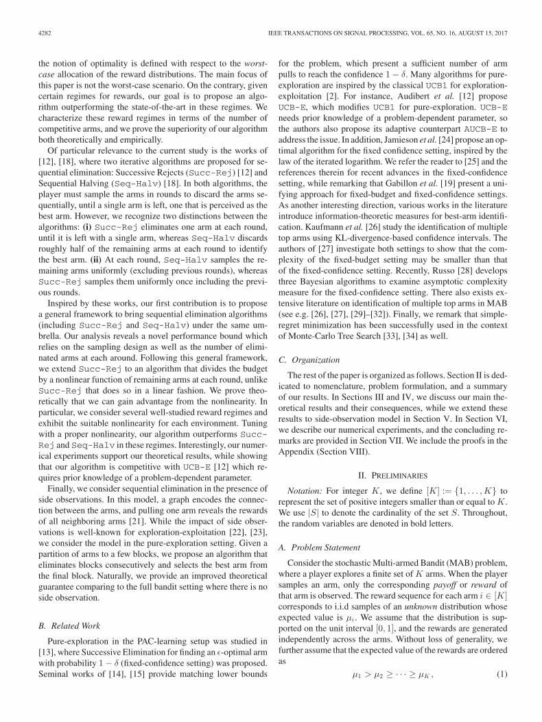
In this section, we propose our generic sequential eliminationmethod and analyze its performance in the fixed budget setting.Consider a sequential elimination algorithm given budget T ofarm pulls. The algorithm maintains an active set initialized bythe K arms, and it proceeds for R rounds to discard the arms se-quentially until it is left by a single arm. Let us use �·� to denotethe ceiling function. Then, for a constant C and a decreas-ing, positive sequence {zr}R

r=1 , set nr = �(T − K)/(Czr )� atround r ∈ [R], let the algorithm sample the remaining arms fornr − nr−1 times, and calculate the empirical average of rewardsfor each arm. If the algorithm dismisses br arms with lowest av-erage rewards, and we impose the constraint

∑Rr=1 br = K − 1

on the sequence {br}Rr=1 , the algorithm outputs a single arm,

the one that it hopes to be the best arm. This general point ofview is summarized in Fig. 1 on the left side.

The choice of C in the algorithm (see Fig. 1) must warrantthat the budget constraint (3) holds. When we substitute nr into(3), we get

nR +R∑

r=1

brnr =⌈

T − K

CzR

⌉

+R∑

r=1

br

⌈T − K

Czr

⌉

≤ T − K

CzR+ 1 +

R∑

r=1

br +R∑

r=1

brT − K

Czr

= K +T − K

C

(1zR

+R∑

r=1

br

zr

)

= T,

where in the last line we used the condition∑R

r=1 br = K − 1.The following theorem provides an upper bound on the errorprobability of the algorithm.

Theorem 2: Consider the General Sequential Elimination al-gorithm outlined in Fig. 1. For any r ∈ [R], let br denote thenumber of arms that the algorithm eliminates at round r. Let alsogr := |Gr | =

∑Ri=r bi + 1 be the number of remaining arms at

the start of round r. Given a fixed budget T of arm pulls and the

input sequence {zr}Rr=1 , setting C and {nr}R

r=1 as describedin the algorithm, the misidentification probability satisfiesthe bound,

P (GR+1 �= {1}) ≤

R maxr∈[R ]

{br} exp

(

−T − K

Cminr∈[R ]

{2Δ2

gr + 1 +1

zr

})

.

It is already quite well-known that the sub-optimality Δi ofeach arm i plays a key role in the identification quality; however,an important subsequent of Theorem 2 is that the performance ofany sequential elimination algorithm also relies on the choice ofzr which governs the constant C. In [12], Succ-Rej employszr = K − r + 1, i.e., at each round the remaining arms areplayed equally often in total. This results in C being of orderlog K.

We now use the abstract form of the generic algorithm tospecialize it to Nonlinear Sequential Elimination delineated inFig. 1. The algorithm works with br = 1 and zr = (K − r + 1)p

for a given p > 0, and it is called “nonlinear” since p is not nec-essarily equal to one. The choice of p = 1 reduces the algorithmto Succ-Rej. In Section IV, we prove that in many regimesfor arm gaps, p �= 1 provides better theoretical results, and wefurther exhibit the efficiency in the numerical experiments inSection VI. The following proposition encapsulates the theoret-ical guarantee of the algorithm.

Proposition 3: Let the Nonlinear Sequential Elimination al-gorithm in Fig. 1 run for a given p > 0, and let Cp and H(p) beas defined in (5). Then, the misidentification probability satisfiesthe bound,

P (GK �= {1}) ≤ (K − 1) exp(

−2T − K

CpH(p)

)

.

The performance of the algorithm does depend on the parameterp, but the choice is more qualitative rather than quantitative.For instance, if the sub-optimal arms are almost the same, i.e.,Δi ≈ Δ for i ∈ [K], noting the definition of Cp and H(p) in(5), we observe that 0 < p < 1 performs better than p > 1. Ingeneral, larger values for p increase H(p) and decrease C(p).Therefore, there is a trade-off in choosing p. We elaborate onthis issue in Sections IV and VI, where we observe that a widerange of values for p can be used for tuning, and the trade-offcan be addressed using either 0 < p < 1 or 1 < p ≤ 2.

We remark that in the proof of Theorem 2, the constant behindthe exponent can be improved if one can avoid the union bounds.To do so, one needs to assume some structure in the sequence{gr}R

r=1 . For instance, the authors in [18] leverage the fact that


Fig. 1. The algorithm on the left represents a general recipe for sequential elimination, whereas the one on the right is a special case of the left hand side, whichextends Succ-Rej to nonlinear budget allocation.

gr+1 = �gr/2� to avoid union bounds in Seq-Halv. The ideacan be extended to when the ratio of gr+1/gr is a constantindependent of r.

Finally, while the result of Proposition 3 provides a generalperformance bound with respect to reward regimes, in the nextsection, we provide two important corollaries of the propositionto study several regimes for rewards, where we can simplify thebound and compare our result with other algorithms.

IV. PERFORMANCE IN SEVERAL SUB-OPTIMALITY REGIMES

Inspired by numerical experiments carried out in the pre-vious works [12], [18], we consider a few instances for sub-optimality of arms in this section, and we demonstrate howN-Seq-El fares in these cases. We would like to distinguishthree general regimes that encompass interesting settings forsub-optimality and determine the values of p for which we ex-pect N-Seq-El to achieve faster identification rates:

1) Arithmetic progression of gaps: In this case, Δi = (i − 1)Δ0 for i > 1, where Δ0 is a constant.

2) A large group of competitive, suboptimal arms: We recog-nize this case as when there exists a constant1 ε ≥ 0 suchthat Δi/Δ2 ≤ 1 + ε for arms i ∈ S, where |S| grows lin-early as a function of K, and for i /∈ S, Δi/Δ2 ≥ i.

3) A small group of competitive, suboptimal arms: Thiscase occurs when there exists a constant ε ≥ 0 such thatΔi/Δ2 ≤ 1 + ε for i ∈ S, where |S| is of constant orderwith respect to K, and for i /∈ S, Δi/Δ2 ≥ i.

We now state the following corollary of Proposition 3, whichproves to be useful for our numerical evaluations. Note that theorders are expressed with respect to K.

1The choice of ε must be constant with respect to i and K .

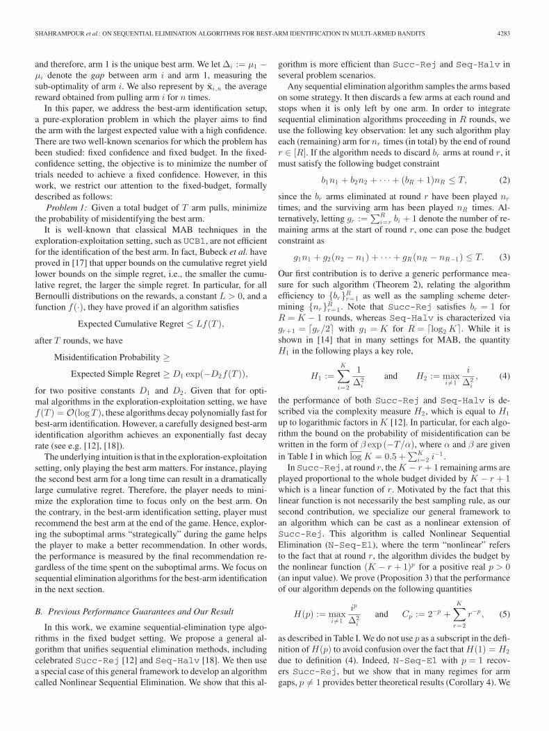
Corollary 4: Consider the Nonlinear Sequential Eliminationalgorithm described in Fig. 1. Let constants p and q be chosensuch that 1 < p ≤ 2 and 0 < q < 1. Then, for the three settingsgiven above, the bound on the misidentification probability pre-sented in Proposition 3 satisfies

We can now compare our algorithm with Succ-Rej andSeq-Halv using the result of Corollary 4. Returning to Table Iand calculating H2 for Regimes 1 to 3, we can observe thefollowing table, which shows that with a right choice of p forN-Seq-El, we can save a O(log K) factor in the exponentialrate comparing to other methods. Though we do not have aprior information on gaps to categorize them into one of theRegimes 1 to 3 (and then choose p), the choice of p is morequalitative rather than quantitative. Roughly speaking: if thesub-optimal arms are almost the same 0 < p < 1 performs betterthan p > 1, and if there are a few real competitive arms, p > 1outperforms 0 < p < 1. Therefore, the result of Corollary 4 is ofpractical interest, and we will show using numerical experiments(Section VI) that a wide range of values for p can potentiallyresult in efficient algorithms.

One should observe that the number of competitive arms isa key factor in tuning p. We now provide another corollary ofProposition 3, which presents the suitable range of parameter pgiven the growth rate of competitive arms as follows.

Corollary 5: Let the number of competitive arms be an arbi-trary function fK of total arms, i.e., there exists a constant ε ≥ 0such that Δi/Δ2 ≤ 1 + ε for i ∈ S, where |S| = fK , and fori /∈ S, Δi/Δ2 ≥ i. Then, there exists a suitable choice of p forwhich N-Seq-El outperforms Succ-Rej and Seq-Halv in


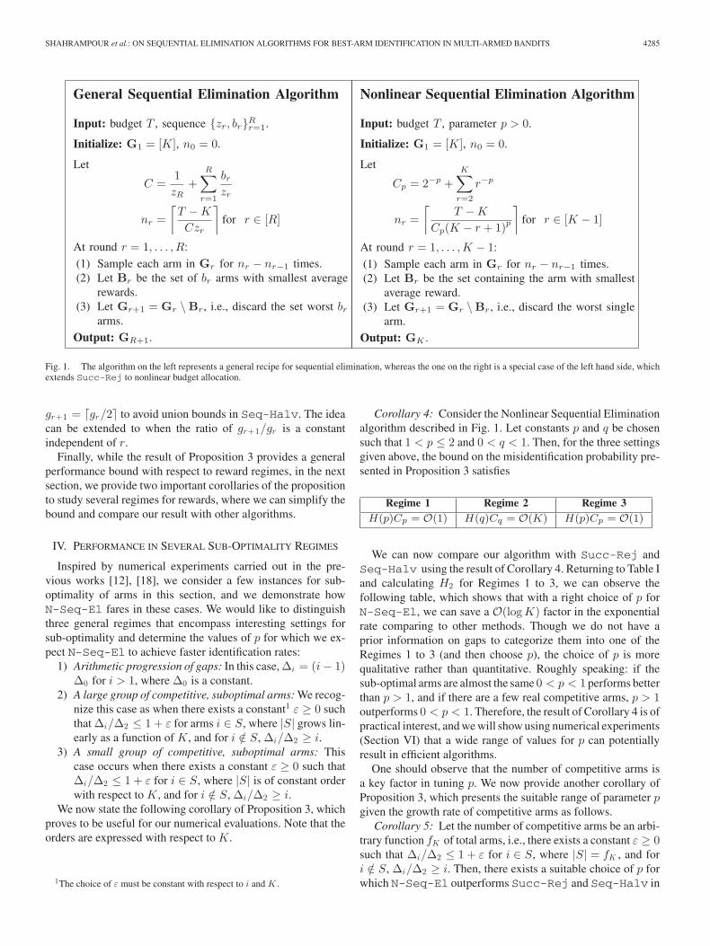
TABLE IITHE MISIDENTIFICATION PROBABILITY FOR ALL THREE ALGORITHMS

DECAYS IN THE FORM OF β exp (−T/α). THE TABLE REPRESENTS THE

PARAMETER α FOR EACH ALGORITHM IN REGIMES 1 TO 3. FOR REGIME 2,WE SET 0 < p < 1, AND FOR REGIMES 1 AND 3, WE USE 1 < p ≤ 2

TABLE IIIGIVEN THAT THE MISIDENTIFICATION PROBABILITY DECAYS IN THE FORM OF

β exp (−T/α), THE TABLE REPRESENTS THE CHOICE OF p FOR WHICH

THE PARAMETER α IN N-Seq-El IS SMALLER THAN THOSE

OF Succ-Rej AND Seq-Halv. NOTE THAT WE USE

lK := max{0, 1 − log(log K )/ log (K/fK )} AND

uK := min{2, 1 + log(log K )/ log(fK )}

TABLE IVTHE TABLE SHOWS THE SUITABLE INTERVAL OF p FOR

K ∈ {40, 120, 5 × 102 , 5 × 104 , 5 × 106 , 5 × 108} GIVEN THE GROWTH

RATE OF COMPETITIVE ARMS AS DERIVED IN COROLLARY 5

the sense that the misidentification probability decays witha faster rate, i.e., we have O(H(p)Cp) ≤ O(H2 log K). Fordifferent conditions on the growth of fK , the suitable choice ofparameter p is presented in Table III.

The corollary above indicates that a side information in theform of the number of competitive arms (in the order) can helpus tune the input parameter p. The corollary exhibits a smoothinterpolation between when the competitive arms are small ver-sus when they are large. Perhaps, the most interesting regimeis the middle row, where the choice of p is given as a func-tion of the number of arms K. Consider the following exam-ple where we calculate the choice of p for fK = Kγ , whereγ ∈ {0.3, 0.5, 0.7}.

As we can see in Table IV, since the condition on p dependsin logarithmic orders on K and fK , we have flexibility to tunep even for very large K. However, we only use K ∈ {40, 120}for the numerical experiments in Section VI, since the time-

complexity of Monte Carlo simulations is prohibitive on largenumber of arms.

V. SIDE OBSERVATIONS

In the previous sections, we considered a scenario in whichpulling an arm yields only the reward of the chosen arm. How-ever, there exist applications where pulling an arm can addition-ally result in some side observations. For a motivative example,consider the problem of web advertising, where an ad placeroffers an ad to a user and receives a reward only if the userclicks on the ad. In this example, if the user clicks on a va-cation ad, the ad placer receives the side information that theuser could have also clicked on ads for rental cars. The value ofside observations in the stochastic MAB was studied in [22] forexploration-exploitation setting. The side-observation model isdescribed via an undirected graph that captures the relation-ship between the arms. Once an arm is pulled, the player ob-serves the reward of the arm as well as its neighboring arms.In exploration-exploitation settings, the analysis of MAB withside observations relies on the cliques of the graph [21], [22].In this section, we would like to consider the impact in thepure-exploration setting.

In the pure-exploration, we minimize the simple regret ratherthan the cumulative regret, and therefore, the player’s best betsare the most connected arms resulting in more observations.Now consider a partition of the set [K] into M blocks {Vi}M

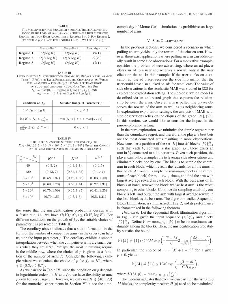
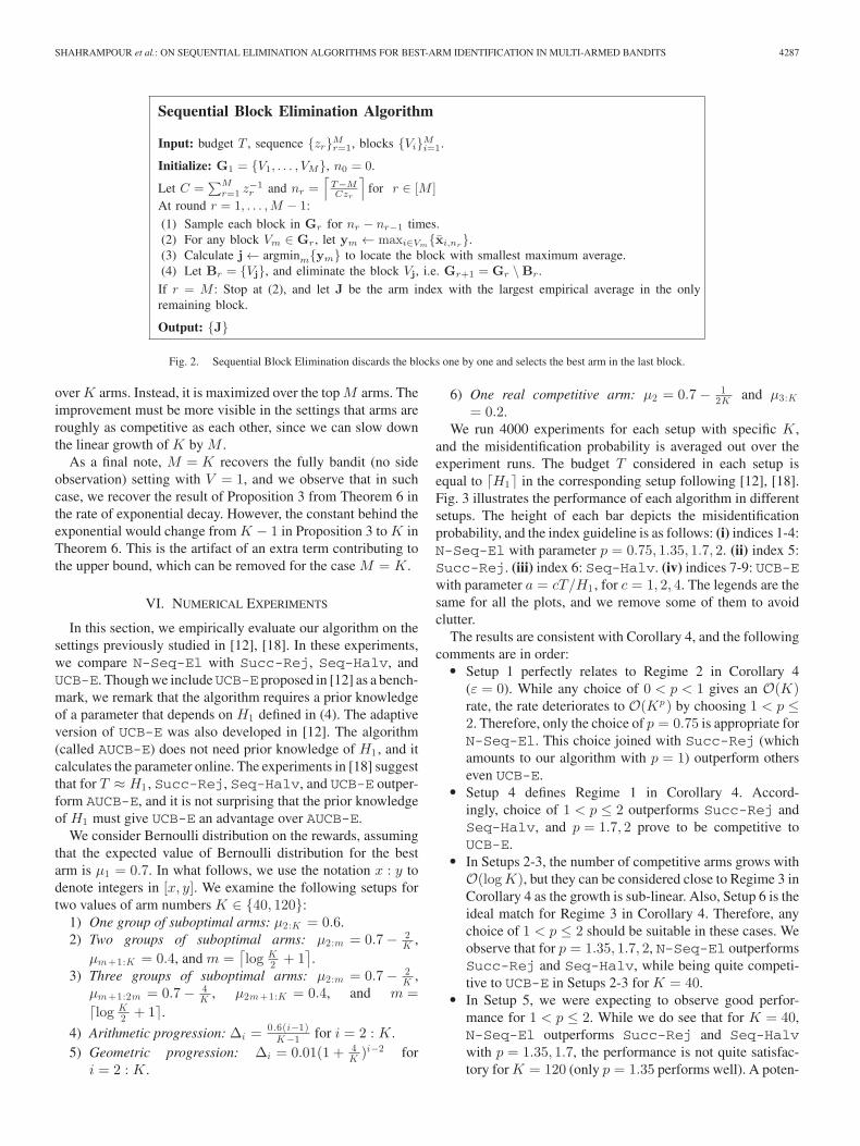
i=1such that each Vi contains a star graph, i.e., there exists anarm in Vi connected to all other arms. Given such partition, theplayer can follow a simple rule to leverage side observations andeliminate blocks one by one. The idea is to sample the centralarm in each block, which reveals the rewards for all the arms inthat block. At round r, sample the remaining blocks (the centralarms of each block) for nr − nr−1 times, and find the arm withlargest average reward in each block. With the best arms of allblocks at hand, remove the block whose best arm is the worstcomparing to other blocks. Continue the sampling until only oneblock is left, and output the arm with largest average reward inthe final block as the best arm. The algorithm, called SequentialBlock Elimination, is summarized in Fig. 2, and its performanceis characterized in the following theorem.

Theorem 6: Let the Sequential Block Elimination algorithmin Fig. 2 run given the input sequence {zr}M

r=1 and blocks{Vi}M

i=1 . Define V := maxi∈[M ]{|Vi |} to be the maximum car-dinality among the blocks. Then, the misidentification probabil-ity satisfies the bound

P ({J} �= {1}) ≤ V M exp(

−T − M

C2 min

r∈[M ]

{Δ2

M +1−r

zr

})

.

In particular, the choice of zr = (M + 1 − r)p for a givenp > 0, yields

P ({J} �= {1}) ≤ V M exp(

−2T − M

CHM,p

)

,

where H(M,p) := maxi∈[M ]\{1}{ ip

Δ2i}.

The theorem indicates that once we can partition the arms intoM blocks, the complexity measure H(p) need not be maximized


Fig. 2. Sequential Block Elimination discards the blocks one by one and selects the best arm in the last block.

over K arms. Instead, it is maximized over the top M arms. Theimprovement must be more visible in the settings that arms areroughly as competitive as each other, since we can slow downthe linear growth of K by M .

As a final note, M = K recovers the fully bandit (no sideobservation) setting with V = 1, and we observe that in suchcase, we recover the result of Proposition 3 from Theorem 6 inthe rate of exponential decay. However, the constant behind theexponential would change from K − 1 in Proposition 3 to K inTheorem 6. This is the artifact of an extra term contributing tothe upper bound, which can be removed for the case M = K.

VI. NUMERICAL EXPERIMENTS

In this section, we empirically evaluate our algorithm on thesettings previously studied in [12], [18]. In these experiments,we compare N-Seq-El with Succ-Rej, Seq-Halv, andUCB-E. Though we includeUCB-E proposed in [12] as a bench-mark, we remark that the algorithm requires a prior knowledgeof a parameter that depends on H1 defined in (4). The adaptiveversion of UCB-E was also developed in [12]. The algorithm(called AUCB-E) does not need prior knowledge of H1 , and itcalculates the parameter online. The experiments in [18] suggestthat for T ≈ H1 , Succ-Rej, Seq-Halv, and UCB-E outper-form AUCB-E, and it is not surprising that the prior knowledgeof H1 must give UCB-E an advantage over AUCB-E.

We consider Bernoulli distribution on the rewards, assumingthat the expected value of Bernoulli distribution for the bestarm is μ1 = 0.7. In what follows, we use the notation x : y todenote integers in [x, y]. We examine the following setups fortwo values of arm numbers K ∈ {40, 120}:

1) One group of suboptimal arms: μ2:K = 0.6.2) Two groups of suboptimal arms: μ2:m = 0.7 − 2

K ,μm+1:K = 0.4, and m =

⌈log K

2 + 1⌉.

3) Three groups of suboptimal arms: μ2:m = 0.7 − 2K ,

μm+1:2m = 0.7 − 4K , μ2m+1:K = 0.4, and m =

�log K2 + 1�.

4) Arithmetic progression: Δi = 0.6(i−1)K−1 for i = 2 : K.

5) Geometric progression: Δi = 0.01(1 + 4K )i−2 for

i = 2 : K.

6) One real competitive arm: μ2 = 0.7 − 12K and μ3:K

= 0.2.We run 4000 experiments for each setup with specific K,

and the misidentification probability is averaged out over theexperiment runs. The budget T considered in each setup isequal to �H1� in the corresponding setup following [12], [18].Fig. 3 illustrates the performance of each algorithm in differentsetups. The height of each bar depicts the misidentificationprobability, and the index guideline is as follows: (i) indices 1-4:N-Seq-El with parameter p = 0.75, 1.35, 1.7, 2. (ii) index 5:Succ-Rej. (iii) index 6: Seq-Halv. (iv) indices 7-9: UCB-Ewith parameter a = cT/H1 , for c = 1, 2, 4. The legends are thesame for all the plots, and we remove some of them to avoidclutter.

The results are consistent with Corollary 4, and the followingcomments are in order:

� Setup 1 perfectly relates to Regime 2 in Corollary 4(ε = 0). While any choice of 0 < p < 1 gives an O(K)rate, the rate deteriorates to O(Kp) by choosing 1 < p ≤2. Therefore, only the choice of p = 0.75 is appropriate forN-Seq-El. This choice joined with Succ-Rej (whichamounts to our algorithm with p = 1) outperform otherseven UCB-E.

� Setup 4 defines Regime 1 in Corollary 4. Accord-ingly, choice of 1 < p ≤ 2 outperforms Succ-Rej andSeq-Halv, and p = 1.7, 2 prove to be competitive toUCB-E.

� In Setups 2-3, the number of competitive arms grows withO(log K), but they can be considered close to Regime 3 inCorollary 4 as the growth is sub-linear. Also, Setup 6 is theideal match for Regime 3 in Corollary 4. Therefore, anychoice of 1 < p ≤ 2 should be suitable in these cases. Weobserve that for p = 1.35, 1.7, 2, N-Seq-El outperformsSucc-Rej and Seq-Halv, while being quite competi-tive to UCB-E in Setups 2-3 for K = 40.

� In Setup 5, we were expecting to observe good perfor-mance for 1 < p ≤ 2. While we do see that for K = 40,N-Seq-El outperforms Succ-Rej and Seq-Halvwith p = 1.35, 1.7, the performance is not quite satisfac-tory for K = 120 (only p = 1.35 performs well). A poten-


Fig. 3. The figure shows the misidentification probability for N-Seq-El, Succ-Rej, Seq-Halv, and UCB-E algorithms in six different setups. The sixplots on the left hand side relate to the case K = 40, and the six plots on the right hand side are associated with K = 120. The height of each bar depicts themisidentification probability, and each index (or color) represents one algorithm tuned with a specific parameter in case the algorithm is parameter dependent.

tial reason is that we want to keep the rewards bounded in[0, 1], thereby choosing the geometric rate for Δi so slowthat it is dominated by ip rate in (5). To support our argu-ment, we present a complementary evaluation of this casefor a small K, where we can use faster geometric growth.

� As a final remark, note that in consistent with Table II,for relevant cases we observe an improvement of perfor-mance when K increases. For instance, in Setup 1 with p =0.75, the ratio of misidentification probability of N-Seq-El to Seq-Halv increases from 1.84 (K = 40) to 2.06


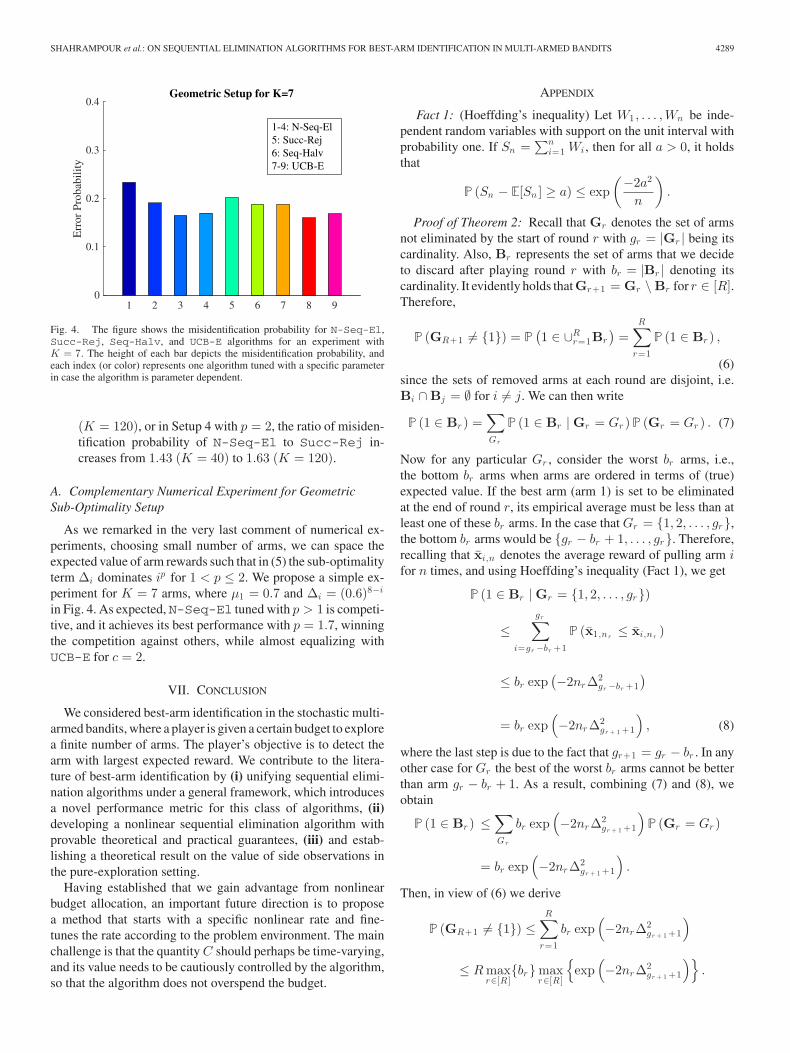
Fig. 4. The figure shows the misidentification probability for N-Seq-El,Succ-Rej, Seq-Halv, and UCB-E algorithms for an experiment withK = 7. The height of each bar depicts the misidentification probability, andeach index (or color) represents one algorithm tuned with a specific parameterin case the algorithm is parameter dependent.

(K = 120), or in Setup 4 with p = 2, the ratio of misiden-tification probability of N-Seq-El to Succ-Rej in-creases from 1.43 (K = 40) to 1.63 (K = 120).

A. Complementary Numerical Experiment for GeometricSub-Optimality Setup

As we remarked in the very last comment of numerical ex-periments, choosing small number of arms, we can space theexpected value of arm rewards such that in (5) the sub-optimalityterm Δi dominates ip for 1 < p ≤ 2. We propose a simple ex-periment for K = 7 arms, where μ1 = 0.7 and Δi = (0.6)8−i

in Fig. 4. As expected, N-Seq-El tuned with p > 1 is competi-tive, and it achieves its best performance with p = 1.7, winningthe competition against others, while almost equalizing withUCB-E for c = 2.

VII. CONCLUSION

We considered best-arm identification in the stochastic multi-armed bandits, where a player is given a certain budget to explorea finite number of arms. The player’s objective is to detect thearm with largest expected reward. We contribute to the litera-ture of best-arm identification by (i) unifying sequential elimi-nation algorithms under a general framework, which introducesa novel performance metric for this class of algorithms, (ii)developing a nonlinear sequential elimination algorithm withprovable theoretical and practical guarantees, (iii) and estab-lishing a theoretical result on the value of side observations inthe pure-exploration setting.

Having established that we gain advantage from nonlinearbudget allocation, an important future direction is to proposea method that starts with a specific nonlinear rate and fine-tunes the rate according to the problem environment. The mainchallenge is that the quantity C should perhaps be time-varying,and its value needs to be cautiously controlled by the algorithm,so that the algorithm does not overspend the budget.

APPENDIX

Fact 1: (Hoeffding’s inequality) Let W1 , . . . , Wn be inde-pendent random variables with support on the unit interval withprobability one. If Sn =

∑ni=1 Wi , then for all a > 0, it holds

that

P (Sn − E[Sn ] ≥ a) ≤ exp(−2a2

n

)

.

Proof of Theorem 2: Recall that Gr denotes the set of armsnot eliminated by the start of round r with gr = |Gr | being itscardinality. Also, Br represents the set of arms that we decideto discard after playing round r with br = |Br | denoting itscardinality. It evidently holds thatGr+1 = Gr \ Br for r ∈ [R].Therefore,

P (GR+1 �= {1}) = P(1 ∈ ∪R

r=1Br

)=

R∑

r=1

P (1 ∈ Br ) ,

(6)since the sets of removed arms at each round are disjoint, i.e.Bi ∩ Bj = ∅ for i �= j. We can then write

P (1 ∈ Br ) =∑

Gr

P (1 ∈ Br | Gr = Gr ) P (Gr = Gr ) . (7)

Now for any particular Gr , consider the worst br arms, i.e.,the bottom br arms when arms are ordered in terms of (true)expected value. If the best arm (arm 1) is set to be eliminatedat the end of round r, its empirical average must be less than atleast one of these br arms. In the case that Gr = {1, 2, . . . , gr},the bottom br arms would be {gr − br + 1, . . . , gr}. Therefore,recalling that xi,n denotes the average reward of pulling arm ifor n times, and using Hoeffding’s inequality (Fact 1), we get

P (1 ∈ Br | Gr = {1, 2, . . . , gr})

≤gr∑

i=gr −br +1

P (x1,nr≤ xi,nr

)

≤ br exp(−2nrΔ2

gr −br +1)

= br exp(−2nrΔ2

gr + 1 +1

), (8)

where the last step is due to the fact that gr+1 = gr − br . In anyother case for Gr the best of the worst br arms cannot be betterthan arm gr − br + 1. As a result, combining (7) and (8), weobtain

P (1 ∈ Br ) ≤∑

Gr

br exp(−2nrΔ2

gr + 1 +1

)P (Gr = Gr )

= br exp(−2nrΔ2

gr + 1 +1

).

Then, in view of (6) we derive

P (GR+1 �= {1}) ≤R∑

r=1

br exp(−2nrΔ2

gr + 1 +1

)

≤ R maxr∈[R ]

{br}maxr∈[R ]

{exp

(−2nrΔ2

gr + 1 +1

)}.


Noting the fact that nr =⌈

T −KC zr

⌉≥ T −K

C zr, we can use above to

conclude that

P (GR+1 �= {1})

≤ R maxr∈[R ]

{br}maxr∈[R ]

{

exp(

−T − K

Czr2Δ2

gr + 1 +1

)}

,

which completes the proof. �Proof of Proposition 3: We point out that the algorithm is

a special case of General Sequential Elimination where R =K − 1, br = 1, gr = K − r + 1, and zr = (K − r + 1)p . Theproof then follows immediately from the result of Theorem 2.�

Proof of Corollary 4: The proof follows by substituting eachcase in (5). We need to understand the order of Cp and H(p) fordifferent regimes of p. Let us start by

Cp = 2−p +K∑

r=2

r−p ,

and noting that for any p > 1, Cp is a convergent sum whenK → ∞. Therefore, for the regime p > 1, the sum is a constant,i.e., Cp = O(1). On the other hand, consider q ∈ (0, 1), andnote that the sum is divergent, and for large K we have Cq =O(K1−q ). Now, let us analyze

H(p) = maxi �=1

ip

Δ2i

.

For Regime 1, since Δi = (i − 1)Δ0 , for p ∈ (1, 2), we have

H(p) = maxi �=1

(

1 +1

i − 1

)p (i − 1)p−2

Δ20

≤ maxi �=1

(

1 +1

i − 1

)p 1Δ2

0=

1.5p

Δ20

,

which is of constant order with respect to K. Therefore, theproduct CpH(p) = O(1).

For Regime 2, we have

H(q) = maxi �=1

iq

Δ2i

≤ maxi �=1

iq

Δ22≤ Kq

Δ22,

and the maximum order can be achieved as the number of armsclose to the second best arm grows linearly in K. Combiningwith Cq = O(K1−q ), the product CqH(q) = O(K).

For Regime 3, if i ∈ S, we have

maxi∈S

ip

Δ2i

= O(1),

since the cardinality of S is of constant order with respect to K.On the other hand, since 1 < p ≤ 2, we have

maxi /∈S

ip

Δ2i

≤ maxi /∈S

ip

i2Δ22

= maxi /∈S

ip−2

Δ22

= O(1).

Therefore, H(p) is of constant order, and combining with Cp =O(1), the product CpH(p) = O(1). �

Proof of Corollary 5: According to calculations in the pre-vious proof, we have that Cp = O(K1−p) for 0 < p < 1, andCp = O(1) for 1 < p ≤ 2. In order to find out the order of H(p)and H2 , we should note that

O(H(p)) = O(

maxi∈S

ip

Δ2i

)

= O(

maxi∈S

ip

Δ22

)

= fpK ,

and we simply have O(H2) = O(H(1)) = fK . Now return-ing to Table I, we must compare O(H(p)Cp) = fp

KO(Cp)and O(H2 log K) = fK log K for all three the rows given inTable III.

Row 1: In the case that 1 ≤ fK ≤ log K, for any choice of1 < p ≤ 2, since Cp = O(1), we always have

fpK ≤ fK log K ⇔ fp−1

K ≤ log K.

Row 3: In the case that Klog K ≤ fK ≤ K − 1, for any choice

of 0 < p < 1, since Cp = O(K1−p), we have

fpKO(Cp) = fp

K K1−p = fK

(K

fK

)1−p

≤ fK log K.

Row 2: In this case, we have that log K < fK < Klog K . To

prove the claim in the Table III, we have to break down theanalysis into two cases:

Row 2 – Case 1: First, consider the case 1 − log log K

log(

Kf K

) <p<1.

Since Cp = O(K1−p), we have that

fpKO(Cp) = fp

K K1−p = fK

(K

fK

)1−p

≤ fK

(K

fK

) l o g lo g K

l o g(

Kf K

)

= fK log K.

Row 2 – Case 2: Second, consider the case 1 < p < 1 +log log Klog fK

. Since Cp = O(1), we have that

fpKO(Cp) = fp

K ≤ f1+ lo g lo g K

l o g f K

K = fK fl o g lo g Kl o g f K

K = fK log K.

Therefore, for all of the conditions on fK , we showed properchoice of p which guarantees fp

KO(Cp) ≤ fK log K. �Proof of Theorem 6: Recall that the elements of Gr are the

set of M + 1 − r blocks not eliminated by the start of roundr ∈ [M ], and Br only contains the block we decide to discardafter playing round r. Also, recall that arm 1 is the best arm,located in the block V1 , and V := maxi∈[M ]{|Vi |} denotes themaximum cardinality of the blocks.

If the algorithm does not output the best arm, the arm is eithereliminated with block V1 in one the rounds in [M − 1], or notselected at the final round M . Therefore,

P (J �= 1) ≤ P(argmaxi∈V1

{xi,nM} �= 1 | GM = {V1}

)

+M −1∑

r=1

P (Br = {V1}) . (9)


The first term can be bounded simply by Hoeffding’s inequality

P(argmaxi∈V1

{xi,nM} �= 1 | GM = {V1}

)

≤ |V1 | exp(−2nM Δ2

2)

= |V1 | exp(−2nM Δ2

1), (10)

using the convention Δ1 := Δ2 . On the other hand, for anyr ∈ [M − 1]

P (Br = {V1})

=∑

Gr

P (Br = {V1} | Gr = Gr ) P (Gr = Gr ) . (11)

Note that, without loss of generality, we sort the blocks basedon their best arm as

μ1 = maxi∈V1

μi > maxi∈V2

μi ≥ · · · ≥ maxi∈VM

μi,

so the best possible arm in Vm cannot be better than armm in view of above and (1). We remove block V1 after ex-ecution of round r only if it is the worst among all othercandidates. Therefore, consider the particular case that Gr ={V1 , V2 , . . . , VM +1−r} contains the best possible M + 1 − rblocks that one can keep until the start of round r. In such case,

P (Br = {V1} | Gr = {V1 , V2 , . . . , VM +1−r})≤ V exp

(−2nrΔ2M +1−r

).

In any other case for Gr the best possible arm in the worst blockcannot be better than arm M + 1 − r. Therefore, combiningabove with (11), we obtain

P (Br = {V1}) ≤ V∑

Gr

exp(−2nrΔ2

M +1−r

)P (Gr = Gr )

= V exp(−2nrΔ2

M +1−r

).

Incorporating above and (10) into (9), we derive

P (J �= 1) ≤ |V1 | exp(−2nM Δ2

1)

+M −1∑

r=1

V exp(−2nrΔ2

M +1−r

)

≤ V

M∑

r=1

exp(−2nrΔ2

M +1−r

)

≤ V M exp(

−T − M

C2 min

r∈[M ]

{Δ2

M +1−r

zr

})

,

noticing the choice of nr in the algorithm (Fig. 2). Having fin-ished the first part of the proof, when we set zr = (M + 1 − r)p

for r ∈ [M − 1] and zM = 2p , we have

P (J �= 1) ≤ V M exp(

−2T − M

CHM,p

)

,

where H(M,p) := maxi∈[M ]\{1}{ ip

Δ2i}. �

ACKNOWLEDGMENT

The authors would like to thank Prof. M. Yukawa (Keio Uni-versity) for his helpful comments during the review process,and also Dr. A. Beirami and Dr. H. Farhadi for many helpfuldiscussions.

REFERENCES

[1] T. L. Lai and H. Robbins, “Asymptotically efficient adaptive allocationrules,” Adv. Appl. Math., vol. 6, no. 1, pp. 4–22, 1985.

[2] P. Auer, N. Cesa-Bianchi, and P. Fischer, “Finite-time analysis of themultiarmed bandit problem,” Mach. Learn., vol. 47, no. 2–3, pp. 235–256, 2002.

[3] P. Auer, N. Cesa-Bianchi, Y. Freund, and R. E. Schapire, “The non-stochastic multiarmed bandit problem,” SIAM J. Comput., vol. 32, no. 1,pp. 48–77, 2002.

[4] S. Bubeck and N. Cesa-Bianchi, “Regret analysis of stochastic and non-stochastic multi-armed bandit problems,” Found. Trends Mach. Learn.,vol. 5, no. 1, pp. 1–122, 2012.

[5] A. Mahajan and D. Teneketzis, “Multi-armed bandit problems,” in Founda-tions and Applications of Sensor Management. Berlin, Germany: Springer-Verlag, pp. 121–151, 2008.

[6] K. Liu and Q. Zhao, “Distributed learning in multi-armed bandit withmultiple players,” IEEE Trans. Signal Process., vol. 58, no. 11, pp. 5667–5681, Nov. 2010.

[7] K. Wang and L. Chen, “On optimality of myopic policy for restless multi-armed bandit problem: An axiomatic approach,” IEEE Trans. Signal Pro-cess., vol. 60, no. 1, pp. 300–309, Jan. 2012.

[8] S. Vakili, K. Liu, and Q. Zhao, “Deterministic sequencing of explorationand exploitation for multi-armed bandit problems,” IEEE J. Sel. Top.Signal Process., vol. 7, no. 5, pp. 759–767, Oct. 2013.

[9] D. Kalathil, N. Nayyar, and R. Jain, “Decentralized learning for mul-tiplayer multiarmed bandits,” IEEE Trans. Inf. Theory, vol. 60, no. 4,pp. 2331–2345, Apr. 2014.

[10] S. Bagheri and A. Scaglione, “The restless multi-armed bandit formula-tion of the cognitive compressive sensing problem,” IEEE Trans. SignalProcess., vol. 63, no. 5, pp. 1183–1198, Mar. 2015.

[11] K. Kanoun, C. Tekin, D. Atienza, and M. Van Der Schaar, “Big-data streaming applications scheduling based on staged multi-armedbandits,” IEEE Trans. Comput., vol. 65, no. 12, pp. 3591–3605,Dec. 2016.

[12] J.-Y. Audibert and S. Bubeck, “Best arm identification in multi-armedbandits,” in Proc. 23rd Conf. Learn. Theory, 2010.

[13] E. Even-Dar, S. Mannor, and Y. Mansour, “PAC bounds for multi-armedbandit and Markov decision processes,” in Proc. Comput. Learn. Theory.Berlin, Germany: Springer-Verlag, 2002, pp. 255–270.

[14] S. Mannor and J. N. Tsitsiklis, “The sample complexity of exploration inthe multi-armed bandit problem,” J. Mach. Learn. Res., vol. 5, pp. 623–648, 2004.

[15] E. Even-Dar, S. Mannor, and Y. Mansour, “Action elimination andstopping conditions for the multi-armed bandit and reinforcementlearning problems,” J. Mach. Learn. Res., vol. 7, pp. 1079–1105,2006.

[16] S. Bubeck, R. Munos, and G. Stoltz, “Pure exploration in multi-armedbandits problems,” in Algorithmic Learning Theory. Berlin, Germany:Springer-Verlag, 2009, pp. 23–37.

[17] S. Bubeck, R. Munos, and G. Stoltz, “Pure exploration in finitely-armedand continuous-armed bandits,” Theor. Comput. Sci., vol. 412, no. 19,pp. 1832–1852, 2011.

[18] Z. Karnin, T. Koren, and O. Somekh, “Almost optimal exploration in multi-armed bandits,” in Proc. 30th Int. Conf. Mach. Learn., 2013, pp. 1238–1246.

[19] V. Gabillon, M. Ghavamzadeh, and A. Lazaric, “Best arm identification:A unified approach to fixed budget and fixed confidence,” in Proc. Adv.Neural Inf. Process. Syst., 2012, pp. 3212–3220.

[20] A. Carpentier and A. Locatelli, “Tight (lower) bounds for the fixed budgetbest arm identification bandit problem,” in Proc. 29th Annu. Conf. Learn.Theory, 2016, pp. 590–604.

[21] S. Mannor and O. Shamir, “From bandits to experts: On the valueof side-observations,” in Proc. Adv. Neural Inf. Process. Syst., 2011,pp. 684–692.


[22] S. Caron, B. Kveton, M. Lelarge, and S. Bhagat, “Leveraging side ob-servations in stochastic bandits,” in Proc. 28th Conf. Uncertainty Artif.Intell., 2012, pp. 142–151.

[23] S. Buccapatnam, A. Eryilmaz, and N. B. Shroff, “Stochastic bandits withside observations on networks,” in Proc. ACM Int. Conf. Meas. Model.Comput. Syst., 2014, pp. 289–300.

[24] K. Jamieson, M. Malloy, R. Nowak, and S. Bubeck, “lil’UCB: An optimalexploration algorithm for multi-armed bandits,” in Proc. 27th Conf. Learn.Theory, 2014, pp. 423–439.

[25] K. Jamieson and R. Nowak, “Best-arm identification algorithms for multi-armed bandits in the fixed confidence setting,” in Proc. 2014 48th Annu.Conf. Inf. Sci. Syst., 2014, pp. 1–6.

[26] E. Kaufmann and S. Kalyanakrishnan, “Information complexity in banditsubset selection,” in Proc. Conf. Learn. Theory, 2013, pp. 228–251.

[27] E. Kaufmann, O. Cappe, and A. Garivier, “On the complexity of best-arm identification in multi-armed bandit models,” J. Mach. Learn. Res.,vol. 17, no. 1, pp. 1–42, 2016.

[28] D. Russo, “Simple Bayesian algorithms for best arm identification,” inProc. 29th Annu. Conf. Learn. Theory, 2016.

[29] S. Kalyanakrishnan and P. Stone, “Efficient selection of multiple banditarms: Theory and practice,” in Proc. 27th Int. Conf. Mach. Learn., 2010,pp. 511–518.

[30] S. Kalyanakrishnan, A. Tewari, P. Auer, and P. Stone, “PAC subset se-lection in stochastic multi-armed bandits,” in Proc. 29th Int. Conf. Mach.Learn., 2012, pp. 655–662.

[31] S. Bubeck, T. Wang, and N. Viswanathan, “Multiple identifications inmulti-armed bandits,” in Proc. 30th Int. Conf. Mach. Learn., 2013,pp. 258–265.

[32] Y. Zhou, X. Chen, and J. Li, “Optimal PAC multiple arm identificationwith applications to crowdsourcing,” in Proc. 31st Int. Conf. Mach. Learn.,2014, pp. 217–225.

[33] T. Pepels, T. Cazenave, M. H. Winands, and M. Lanctot, “Minimizingsimple and cumulative regret in Monte-Carlo tree search,” in ComputerGames. Berlin, Germany: Springer-Verlag, 2014, pp. 1–15.

[34] Y.-C. Liu and Y. Tsuruoka, “Regulation of exploration for simple regretminimization in Monte-Carlo tree search,” in Proc. IEEE Conf. Comput.Intell. Games, 2015, pp. 35–42.

Shahin Shahrampour received the B.Sc. degreefrom Sharif University of Technology, Tehran, Iran,in 2009 and the M.S.E. degree in electrical engineer-ing, the M.A. degree in statistics, and the Ph.D. degreein electrical and systems engineering from the Uni-versity of Pennsylvania, PA, USA, in 2012, 2014, and2015, respectively. He is currently a Postdoctoral Fel-low in electrical engineering at Harvard University,Cambridge, MA, USA. His research interests includemachine learning, online learning, optimization, anddistributed algorithms.

Mohammad Noshad received the Ph.D. degree inelectrical engineering from the University of Virginia,Charlottesville, VA, USA, in 2013. He was a Postdoc-toral researcher at Harvard University. He is currentlythe Chief Technology Officer at VLNComm, Char-lottesville, VA, USA. His research interests includevisible light communications, free-space optical com-munications, time-series analysis, and machine learn-ing. He received the Best Paper Award at the IEEEGLOBECOM 2012.

Vahid Tarokh is currently a Professor of appliedmathematics, a Senior Research Fellow in electri-cal engineering, and a member of Center for Mathe-matics and Applications at Harvard University, Cam-bridge, MA, USA. In the past, he has published on Liegroups and algebras, lattices, graphical models, pseu-dorandomness, information theory, random matrixtheory, coding, communications, pricing and schedul-ing, statistical signal processing (including adaptivealgorithms) and applications (e.g., MRI and EEG sig-nal processing), radar, and distributed astronomy. His

main research interests include applied and computational mathematics. He hasbeen selected as a Guggenheim Fellow in applied mathematics (for his work onrandom and pseudorandom matrices), and has received four honorary degrees.

Documents

IEEE TRANSACTIONS ON SIGNAL PROCESSING, VOL. 65, NO. 16 ... · Shahin Shahrampour, Mohammad Noshad, and Vahid Tarokh Abstract—We consider the best-arm identiﬁcation problem in