IEEE TRANSACTIONS ON SIGNAL PROCESSING 1 SOI …stergios/papers/TSP06-SOI-KF.pdf · IEEE TRANSACTIONS ON SIGNAL PROCESSING 1 SOI-KF: Distributed Kalman Filtering With Low-Cost Communications

IEEE TRANSACTIONS ON SIGNAL PROCESSING 1

SOI-KF: Distributed Kalman Filtering With Low-CostCommunications Using the Sign of Innovations

Alejandro Ribeiro, Student Member, IEEE, Georgios B. Giannakis, Fellow, IEEE, andStergios I. Roumeliotis, Member, IEEE

Abstract—When dealing with decentralized estimation, it isimportant to reduce the cost of communicating the distributedobservations—a problem receiving revived interest in the contextof wireless sensor networks. In this paper, we derive and analyzedistributed state estimators of dynamical stochastic processes,whereby the low communication cost is effected by requiringthe transmission of a single bit per observation. Following aKalman filtering (KF) approach, we develop recursive algorithmsfor distributed state estimation based on the sign of innovations(SOI). Even though SOI-KF can afford minimal communicationoverhead, we prove that in terms of performance and complexityit comes very close to the clairvoyant KF which is based on theanalog-amplitude observations. Reinforcing our conclusions, weshow that the SOI-KF applied to distributed target tracking basedon distance-only observations yields accurate estimates at lowcommunication cost.

Index Terms—Distributed state estimation, Kalman filter (KF),target tracking, wireless sensor networks.

I. INTRODUCTION

DISTRIBUTED signal processing is a well-appreciatedtoolbox for decentralized tracking applications involving,

e.g., multiple radars, but has received a revived interest recentlyin the context of wireless sensor networks (WSNs) [5]. Unlikecentralized signal processing, observations and the resultantalgorithms are physically distributed across sensors in thenetwork, dictating that intersensor communications should beviewed as an integral part of the problem at hand, be it recon-struction, filtering or estimation. For distributed estimation ofdynamical stochastic processes dealt with in this paper, onlyquantized observations are communicated. Thus, the estimation

Manuscript received August 16, 2005; revised December 19, 2005. Work inthis paper was prepared through collaborative participation in the Communica-tions and Networks Consortium sponsored by the U. S. Army Research Labora-tory under the Collaborative Technology Alliance Program, Cooperative Agree-ment DAAD19-01-2-0011. The U. S. Government is authorized to reproduceand distribute reprints for Government purposes notwithstanding any copyrightnotation thereon. The views and conclusions contained in this document arethose of the authors and should not be interpreted as representing the officialpolicies, either expressed or implied, of the Army Research Laboratory or theU. S. Government. Part of the results in this paper appeared in [27]. The editorcoordinating the review of this manuscript and approving it for publication wasDr. Mounir Ghogho.

Color versions of Figs. 3–10 are available online at http://ieeexplore.ieee.org.A. Ribeiro and G. B. Giannakis are with the Department of Electrical and

Computer Engineering, the University of Minnesota, Minneapolis, MN 55455USA (e-mail: [email protected]; [email protected]).

S. I. Roumeliotis is with the Department of Computer Science and Engi-neering, the University of Minnesota, Minneapolis, MN 55455 USA (e-mail:[email protected]).

Digital Object Identifier 10.1109/TSP.2006.882059

problem is certainly different from state estimation based onthe original (analog-amplitude) observations.

Without explicitly considering quantization, spatial redun-dancy across sensor observations has been exploited to reducecommunication requirements [3], [4], [9], [21], [23], [24].Accounting for quantization, distributed estimation algorithmswere explored in early works, see, e.g., [10] and [17]; andrecently in the context of WSNs. The design of quantizers indifferent scenarios was studied in [22], where the concept of in-formation loss was defined as the relative increase in estimationvariance when using quantized observations with respect tothe equivalent estimation problem based on analog-amplitudeobservations. To address the challenge of building suitablenoise models for WSNs, universal estimators that work irre-spective of the noise distribution were introduced in [18] andshown to have an information loss independent of the networksize. Another insight when estimating signals using very noisysensor data was offered by [25], [26], where it was shown thatas the noise variance becomes comparable with the parameter’sdynamic range, quantization to a single bit per observationleads to low complexity estimators of time-invariant deter-ministic parameters with minimal information loss. This holdstrue for a large class of problems, where the noise probabilitydistribution function (pdf) may be parametrically described oreven unknown [25].

Taking into account the stringent bandwidth constraintsof WSNs, this paper studies state estimation of dynamicalstochastic processes based on severely quantized observations,whereby low-cost communications restrict sensors to transmit asingle bit per observation. The quantization rule manifests itselfin a non-linear measurement equation in a Kalman Filtering(KF) setup. While the discontinuous non-linearity precludesapplication of the extended (E) KF, it can be handled with morepowerful techniques such as the unscented (U) KF [14], or theparticle filter (PF) [7], [16]—algorithms that have also beenapplied in the context of filtering [6], [29] and target trackingwith a WSN [1], [8]. However, all these approaches are signif-icantly more complex than a KF and, besides, no insight hasbeen provided with regards to their performance degradationwhen quantized data are used in lieu of the analog-amplitudeobservations. The contribution of the present paper is preciselyto address these two issues with the goal being to construct stateestimators based on binary observations so that: i) complexityis rendered comparable to the equivalent KF based on theoriginal observations; and ii) the mean squared error (MSE) ofthe resultant estimate based on binary observations is close tothe MSE of the estimate based on the original observations.

1053-587X/$20.00 © 2006 IEEE

2 IEEE TRANSACTIONS ON SIGNAL PROCESSING

We begin by introducing our WSN setup and formulatingthe problem in Section II, where we delineate the KF thatwe will use to benchmark algorithms in the rest of this paper(Section II-A). State estimation based on the sign of innovations(SOI) is considered first for a vector state-scalar observationmodel in Section III, where we discuss the minimum meansquared error (MMSE) estimator (Section III-A). As the lattermay be prohibitive for a resource-limited WSN, we pursuea reduced-complexity approximation in Section III-B whichleads to the SOI-KF algorithm whose complexity and perfor-mance are surprisingly close to the clairvoyant KF, even whenintersensor communication relies on the low-cost transmissionof a single bit per sensor. These results are extended to ageneral vector state-vector parameter model in Section IV. Theperformance of the SOI-KF is analyzed in Section V, whereusing the underlying continuous-time physical processes weshow that the MSE of the SOI-KF is closely related to theMSE of a KF with measurement noise covariance matrix only

times the original one. We present a motivating examplein Section VI, entailing temperature monitoring with a WSN.Finally, we apply a modified version of the SOI-KF to thecanonical problem of distributed target tracking based on bi-nary observations in Section VI-A. Section VII concludes thispaper.

Notation: We use to denote the probability den-sity function (pdf) of the random variable (r.v.) given ther.v. evaluated at ; when using the same letter to denote ther.v. and the argument of the pdf we abbreviate

. When an r.v. is normally distributed with meanand covariance matrix , we write

, where stands for transposition. In the partic-ular case of a scalar r.v., we write anddefine the Gaussian tail function as .We will use to denote the Dirac delta function defined by

, and ; and to denotethe Kronecker delta function defined as and

. For any function the notation willimply that . Throughout this paper, will de-note the identity matrix, and lower (upper) case boldface letterswill stand for column vectors (matrices).

II. PROBLEM STATEMENT AND PRELIMINARIES

We are primarily concerned with so called ad-hoc WSNs inwhich the network itself is responsible for collecting and pro-cessing information; see Fig. 1. Let us consider an ad-hoc WSNwith distributed sensors deployed with the objec-tive of tracking a real random vector (state) .The state evolution in continuous-time is described by

(1)

where , and the driving inputis a zero-mean white Gaussian process with autocorrelation

. The sensors ob-serve the state through a linear transformation. Letting

denote the observation at sensor , we have

(2)

Fig. 1. Ad-hoc WSN: the network itself is in charge of tracking the state x(n).

where and the observation noiseis also a zero-mean Gaussian process with

,i.e., the noise is uncorrelated across time and sensors.

To track , we consider uniform sampling with periodand define the discrete-time state and observations as

and , respectively. Using thecontinuous-time model described by (1) and (2) we can obtainan equivalent discrete-time model [20, Sec. 4.9]. Upon defining

, we can solve the differentialequation in (1) between and with initial condition

to obtain

(3)

For simplicity, define the matrixand the white Gaussian driving noise input

. With these definitions, the re-sultant discrete-time equivalent model is given by the vectortime-varying autoregressive (AR) process

(4)

where and the observation noise iswhite Gaussian with pdf .Since sampling (2) requires passing through a low-or band-pass filter of bandwidth , the sampled covari-ance matrix satisfies

[20, Sec. 4.9]. Finally, note that ’sdefinition implies thatwith covariance matrix

.Supposing that , , and are

available , the goal of the WSN is for each sensor toform an estimate of to be used in e.g., a habitat monitoringapplication [19], or, as a first step in e.g., a distributed controlsetup [13]. In any event, estimating necessitates eachsensor to communicate to the remaining sensors

. This communication takes place over the sharedwireless channel that we will assume can afford transmission

RIBEIRO et al.: SOI-KF: DISTRIBUTED KALMAN FILTERING WITH LOW-COST COMMUNICATIONS 3

of a single packet per time slot , leading to a one-to-one cor-respondence between time and sensor index and allowingus to drop the sensor argument in (4). The decision of whichsensor is active at time , and consequently whichobservation gets transmitted, depends on theunderlying scheduling algorithm—see, e.g., [11], [21]. and thereferences therein—but is assumed given for the purpose ofthis paper. Digital transmission of also implies some formof quantization to map the analog observations intobinary data

with (5)

where is an -component bi-nary message. Implicit to (5) is the fact that we are restricting thesensors to transmit one bit per scalar observation which effectslow-cost communications among sensors. Indeed, the quantiza-tion function partitions in regions, implying that onthe average each component of is quantized to 1 bit. Wefurther suppose that the messages are correctly receivedby all sensors, which assumes deployment of sufficiently pow-erful error-control codes.

The objective of this paper is to derive and analyze the per-formance of MMSE estimators of based on the messages

that are available to each andevery sensor. It is well known that the MMSE estimator is givenby the conditional expectation [15, Ch. 12]; consequently, if welet denote the MMSE estimator of given , wehave

(6)

Instrumental to the ensuing derivations are the so called pre-dictors that estimate (predict) the state and observation vectorsbased on past observations

(7)

For each of the state estimators in (6) and (7), we define theerror covariance matrices (ECM)

, andfor the filtered and the predicted es-

timate, respectively. The mean square errors (MSEs) ofand are given by andwith these traces being minimum among all possible estimators

and of . The ECM of the state predictorcan be obtained from the ECM of the state estimator through therecursion

(8)

which we will use in later derivations. Note that the relationsbetween and and and

in (7) and between andin (8) follow from the linearity of the expected value operatorand are independent of the quantization rule in (5).

Fig. 2. WSN with a fusion center: The sensors act as data gathering devices.

Remark 1: When a fusion center (FC) is present, the WSNis termed hierarchical in the sense that sensors act as informa-tion gathering devices for the FC that is in charge of processingthis information; see Fig. 2. Results in this paper also apply tonetworks of this type provided that the FC feeds back to the sen-sors packets . As we will discuss in Sections III-Band IV, the sole condition for applying the proposed method isto have the predicted observation available at ,a condition that can be met in the hierarchical WSN with feed-back .

A. The Kalman Filter Benchmark

Before considering estimation based on binary observations,let us highlight some properties of the clairvoyant KF that willcome handy in subsequent derivations. Consider for simplicitya vector state-scalar observation model described by

(9)

The model in (9) is a particular case of the general model (4) inwhich ; the observations , noise

and noise covariance are scalar; andis a row vector.

If we had infinite bandwidth available, we could commu-nicate the observations error-free. This is rightfully aclairvoyant benchmark for our bandwidth-constrained estima-tors and corresponds to the problem setup of Section II withmessages . In this case, we have a well knownlinear Gaussian vector AR estimation problem whose MMSEcan be recursively obtained by the KF [15, Ch. 13]. Assumingthat the estimate and the ECMare known at step , we compute the predicted estimate

and the corresponding ECM using(7) and (8), respectively. Next, the filtered estimate isobtained by solving the integral in (6) with the posterior pdfcomputed by means of Bayes’ rule

(10)

The key observation is that because of the linear Gaussian model(9), the posterior isnormal, leading to the so called correction step


(11)

where we defined the innovation sequence. Recursive application of (7), (8) and (11) yields the

MMSE estimate of given .

III. STATE ESTIMATION USING THE SIGN OF INNOVATIONS

The corrector in (11) depends on the innovation sequencecorresponding to the differ-

ence between the current observation and the prediction basedon past observations. This suggests that a convenient form forthe quantization function is . We startby considering the vector state-scalar observation model in (9)and define the message as the SOI

ifif

(12)

Notice that the SOI is not a standard quantizer of the data. It can be thought as one that judiciously sets the quanti-

zation threshold at the data prediction . The focus ofthe present section is to study MMSE estimation of basedon .

A. Exact MMSE Estimator

To find the MMSE in (6) based on the SOI in (12) we can, inprinciple, proceed as we described in Section II-A for the KF.However, while we can update the estimate andits ECM using (7) and (8) to obtain the pre-dictor and its corresponding ECM , theanalogy with the KF cannot be pursued any further. The reasonis that due to the non-linearity in the definition of in (12)the distribution is no longer normal; and, thus,its description requires additional information besides its meanand variance. This characteristic problem of nonlinear filteringmotivates the need for a means of propagating the posterior pdf

so that the integral in (6) can be evaluated. Such arule is described in the following proposition.

Proposition 1: Consider the vector state-scalar observationmodel defined by (9), and the SOI messages defined as in (12).Then, the posterior pdf of given the binary observations

can be obtained using the recursions

(13)

(14)

where is a normalizing constant ensuring that.

Proof: The prior pdf in (13) follows fromthe theorem of total probability

(15)

Note, however, that since is given in, conditioning on

is irrelevant and

yielding (13). The posterior pdf in (14) can be obtained fromBayes’ rule

(16)But the term

can be easily expressed in terms of theGaussian tail function

(17)

where the first equality follows from the definition of the SOIin (12) and the fact that since is given we can ignore

the conditioning on ; the second equality is obtained bysubstituting for the observation model expression in (9);and the last equality is a consequence of the observations’ noisedistribution, .

Substituting (17) into (16) yields (14) after setting.

Two recursive algorithms for computing the MMSEcan be derived from Proposition 1. Algorithm 1-A is run atthe sensors when the scheduling algorithm dictates that is theirturn to transmit the SOI. At this time slot, the sensor com-putes the distribution using (13) from whereit predicts the state value by numerically evaluating

. Based on this prediction,the sensor evaluates as in (7) inorder to obtain and transmit the SOI as defined in (12). Al-gorithm 1-B is run by all sensors during the life of the network tokeep track of the state via the filtered estimate (corrector)

. To this end, all sensors compute the pdfusing (13), and subsequently apply (14) to find .The estimate of interest is obtained by numerical inte-gration of the expression in (6).

Albeit optimal, the process described by Algorithms 1-Aand 1-B requires numerical integration at three different times.We first have to evaluate the integral necessary to obtain

as stated in (13) for step 1 of Algorithm 1-Aand step 2 of Algorithm 2-B. A second numerical integration instep 2 of Algorithm 1-A is required to compute andanother one in step 5 of Algorithm 1-B to compute the desiredestimate, . As these can be prohibitively expensive


for a resource limited WSN, we are motivated to pursue areduced-complexity approximation that we introduce next.

B. Approximate MMSE Estimator

A customary simplification in non-linear filtering is to assumethat the pdf

is Gaussian; see, e.g., [16]. In general, the normal approx-imation of is introduced to reduce the problemof tracking the evolution of a pdf to that of tracking its mean

and covariance . For the problem athand though, it also leads to a very simple algorithm as assertedby the following proposition.

Proposition 2: Consider the vector state-scalar observationmodel in (9) and binary observations defined as in (12). If

, then theMMSE estimator can be obtained from the recursions

(18)

(19)

(20)

(21)

Proof: The predictor recursions (18) and (19) are identicalto (7) and (8), respectively, and are included here for complete-ness. To establish (20), recall that the conditional mean can beobtained by averaging over the posterior pdf :

(22)

Using Bayes’ rule, we can find the posterioras

(23)We now examine the three terms on the right-hand side of(23). The first one is

, which after repeating the steps used toestablish (17) in the proof of Proposition 1 can be expressed interms of the Gaussian tail function

(24)

To obtain an expression for the term, we use the normal assumption on the

distribution of to obtain

(25)where the first equality follows from the definition of in(12). To obtain the second equality note that Gaussianity of

implies that of since is alinear transformation of ; and also that the probability ofa normal variable to be greater or smaller than its mean equals1/2.

Substituting (24) and (25) into (23) and using the (assumed)normal distribution

, we obtain an expression for the posteriordistribution that we substitute in (22) to arrive at

(26)

In the Appendix, we prove that the integral in (26) can be re-duced to (20).

To obtain (21), we writewith the explicit value of as deduced from (20), so that wecan write the ECM as

(27)

where the first equality follows by definition and, in the secondequality, we used that

. The last term in (27) can be furthersimplified after recalling that ,and using the theorem of total probability to obtain

(28)


Substituting (28) into (27) and noting that , weobtain

(29)

which after using the expression for leads to (21).As we commented earlier, the simplification

yields the low-complexity SOI-KF that implements distributedstate estimation based on single-bit observations using therecursions (18)–(21). To estimate , we only require a fewbasic algebraic operations per iteration. Moreover, the SOI-KFrecursion is strikingly reminiscent of the KF recursions (7), (8),and (11). The ECM updates in particular are identical exceptfor the factor in (21).

The algorithmic description of the SOI-KF is summarizedin Algorithm 2-A which is run by the sensors as dictated bythe scheduling algorithm; and Algorithm 2-B which is continu-ously run by all sensors to track . These algorithms are tobe contrasted with their exact MMSE counterparts (Algorithms1-A and 1-B) to note that the numerical integrations have beenreplaced by simple algebraic expressions. Indeed, the SOI-KFobservation and transmission Algorithm 2-A computes the pre-diction by successive application of (18) and (7) tocompute and transmit the SOI in (12). The reception and esti-mation Algorithm 2-B is identical to a KF algorithm except forthe (minor) differences in the update equations.

A few remarks are now in order.Remark 2: It is possible to express the SOI-KF corrector in

(20) in a form that exemplifies its link with the KF corrector in(11). Indeed, if we define the SOI-KF innovation as

(30)we can re-write the SOI-KF corrector as

(31)

Note that (31) is identical to (11) if we replace withthe innovation . Moreover, notethat the units of and are the same, andthat . Even more interesting[cf. (11) and (32)]

(32)

which explains the relationship between the ECM correctionsfor the KF in (11) and for the SOI-KF in (21). The differencebetween (11) and (31) is that in the SOI-KF the magnitude ofthe correction at each step is determined by the magnitude of

and it is the same regardless of how large orsmall the actual innovation is.

Remark 3: As , the Gaussian tail functionconverges uniformly

to 1/2 and, consequently, converges uni-formly to a normal distribution. Thus, the assumption

holdsasymptotically as . For this reason, the SOI-KF yieldsan accurate approximation of the MMSE estimator at lowsignal to noise ratios (SNRs). The accuracy of the approxima-tion decreases as the SNR increases.

Remark 4: When matrices in the state–space model (4) aretime-invariant, it is well known that the KF converges to theWiener filter (WF) as , which, as is also known, can beapproximately implemented by the least-mean-squares (LMS)algorithm. Consequently, one may wonder whether there is a re-lation between the SOI-KF of this paper and the sign-LMS [28,Sec. 5.7]. Apart from offering low complexity versions of theKF and WF, respectively, the two schemes are fundamentallydifferent. In the sign-LMS algorithm, the SOI sequence is usedto recursively update the coefficients of the WF which has asinput the analog-amplitude observations. In the SOI-KF, how-ever, the gain coefficients are computed from the KF correlationmatrices and the SOI sequence is used as the filter input.

IV. VECTOR STATE-VECTOR OBSERVATION CASE

The general vector state-vector observation case defined by(4) can be reduced to the vector state-scalar observation problemconsidered in Section III-B. If the noise vectors are white,i.e., then Proposition 2 can be applied verbatim,for is not more than a collec-tion of independent scalar observations . If

is not white, the idea is to whiten the observations so thatwe can rewrite the problem as a sequence of vector state-scalarobservation problems. To this end, we define the observation

to obtain [c.f. (4)]

(33)

where . For future reference,we write ,

andthat allows us to write (33)

componentwise as


(34)

where the observation noise variance is.Equation (34) has the same form as (9) in the sense that

the state is a vector but the observation isscalar. Mimicking the treatment in Section III, we define

and introduce theMMSE estimator

(35)

which is the MMSE estimator based on past messages and thefirst components of the current message. We adopt the con-vention , and note that

with as defined in (7) andas defined in (6). From (35), we obtain the MMSE predictor of

as [c.f. (34) and (35)]

(36)

From (36), we define the SOI observations for the vector state-vector observation problem as

(37)Setting aside the necessary differences in notation, the problemof finding the MMSE estimator in (35) based on the observationmodel (34) when the binary observations are given by (37) isequivalent to a sequence of MMSE estimation problems forthe vector state-scalar observation model in (9) with binary ob-servations as in (12). An approximate MMSE for this problemwas summarized in Proposition 2 that, with proper notationalmodifications, can now be generalized as follows.

Proposition 3: Consider the vector state-vector obser-vation model defined by (4), binary observations definedas in (37) and letbe defined as [c.f. (33)]. If

, then the MMSE estimate canbe obtained from the recursions

(38)

(39)

(40)

(41)

(42)

where for each time index , steps (40) to (42) are repeatedfor . We adopt the conventions

and , and note that theMMSE estimate and the ECM are given by

and .

Proof: As pointed out earlier, Proposition 3 follows fromrepeated application of Proposition 2. Indeed, if we define thevector the state equation for

can be written as

(43)

On the other hand, the whitened observations can be written as[c.f. (34) with ]

(44)

Define now the MMSE estimatorsand

with corresponding ECMand . Applying

Proposition 2, we obtain the prediction recursions for[c.f. (18), (19), and (43)]

(45)

and for [c.f. (18), (19), and (43)]

(46)

From Proposition 2, we also obtain the correction recursions.Upon defining the gain

(47)the filtered estimate and ECM can be written as [c.f. (20), (21),(44), and (47)]

(48)

Note however, that since for , wehave that and

; and likewise for the ECMs:and

. To obtain (38) and (39), it sufficesto substitute the latter into (45). To obtain (40)–(42), we simplymake these same substitutions in (48) after plugging (46) into(48).

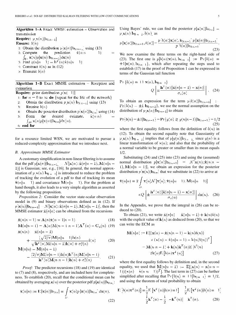
The algorithmic description of the SOI-KF is summarized inAlgorithms 3-A and 3-B. Algorithm 3-A is run at the sensorswhen the scheduling algorithm dictates that it is their turn totransmit an observation. When this happens, the sensor runs thepredictor using (38) and (39) (step 1) and whitens the observa-tion (step 2). Subsequently, it recursively computes par-tial MMSE estimators via (36) and (40)–(42) in order to obtainthe binary observations by means of (37). When thisprocess is complete, the message is transmitted. Interest-ingly enough, when the observations are scalar, Algorithm 3-A


amounts to sequential application of steps 1, 2, 4, 5, and 8; whichis, of course, equivalent to Algorithm 2-A.

Algorithm 3-B is continuously ran by the sensors to estimatethe state . At each time slot we compute the predictorsalong with and move on to process the received mes-sage . Processing of entails recursive application of(40)–(42) for the entries of . After this process is com-plete, we obtain the MMSE estimate .

V. PERFORMANCE ANALYSIS

By definition, any MMSE estimator minimizes the trace ofthe corresponding ECM. Thus, to the extent that the approxi-mationis accurate enough, the SOI-KF in Proposition 2 is optimum inthe sense of minimizing and . How-ever, this optimality does not provide any insight with respect tothe performance of the SOI-KF relative to the MMSE based onthe original observations which are used by the clairvoyant KFin (7), (8), and (11). In this section, we compareand for the SOI-KF with and

reserved to denote the corresponding quan-tities for the KF.

To simplify notation, define . Inter-estingly, is independent of the observations , andregardless of the data we can find by solving the dis-crete-time Ricatti equation that is obtained by substituting theexpression for in (21) into the ECM update for

in (19)

(49)

Likewise, upon defining , we obtainthe discrete-time Ricatti equation for the clairvoyant KF [c.f. (8)and (11)]

(50)

Notice that (49) and (50) differ only by the factor in thenumerator of the ratio in (49). A possible performance com-parison could be to solve the difference (49) and (50) for spe-cific models and compare with . However,better insight can be gained by recalling the underlying contin-uous-time model, for which we start with the following defini-tion.

Definition 1: Consider the continuous-time model (1), (2)and a family of corresponding discrete-time models (4) parame-terized by . Let and be the ECMof the filtered and predicted estimates of the SOI-KF in Propo-sition 2 when sampling period is used in (4). Then, the con-tinuous-time ECM is defined as

(51)

An equivalent definition can be written for the clairvoyant KFwhose continuous-time ECM will be denoted [20]. Ingeneral, the continuous-time MSE is easier to analyze but at thesame time more general since, being independent of the sam-pling time, it provides insights about the fundamental propertiesof the problem. Moreover, it is well known that [20]

(52)Equation (52) reveals that the continuous-time MSE, ,serves as an upper (lower) bound for

. The continuous-time ECMcan be obtained by solving a continuous-time Ricatti equationas we show in the next proposition.

Proposition 4: For the SOI-KF introduced in Proposition 2,consider the continuous-time ECM given by Definition1. Then, can be obtained as the solution of the differentialequation

(53)

Proof: Consider a neighborhood around . To es-tablish (53), it suffices to subtract from both sides of (49),divide by and let . Indeed, the limit of the left-handside of (49) is

(54)


where the first equality follows from the definition ofin (51) and in the second equality, we used the definition ofderivative and set . On the right-hand side, we startwith the limit shown in

(55)

where in the second equality we used the definitions ofand in (51). How-

ever, since , wefind

(56)

Consider now the variance of the driving input whose limit is

(57)

where in obtaining the first equality we used the definition of. To obtain the last equality we applied the mean value

theorem and wrote.

For the remaining term on the right-hand side of (49), wedefine the limit

(58)

where in the second step the key substitution is; and we also used the fact that

, and thedefinition of in (51).

Finally, note that according to (49) and the definitions of ,we have that . Combining this with the limit

expressions in (54), (56), (57) and (58), we obtain (53) afterrearranging terms.

Either repeating Proposition 4 for the KF, or using standardreferences for the continuous-time KF, we know that canbe obtained as the solution of the Ricatti equation [20]

(59)

which is identical to (53) with the substitution. Thus, the continuous-time MSE of the SOI-KF

coincides with the continuous-time MSE of a KF withtimes larger measurement noise variance.

To state an analogous result for the vector state-vector obser-vation SOI-KF of Proposition 3, we will need the definition ofthe -equivalent system that we introduce next.

Definition 2: Consider a state-observation modelas in (1), (2), where the noise autocorrelation is

.We say that a model with otherwise identical parame-ters but noise autocorrelation

, is -equivalent.For a given sampling period , the KF for this latter modelwill be henceforth called the -KF. We will denoteits filtered and predicted ECM as and

and the continuous-time ECM as.

Using Definition 2, we can establish the relationship betweenthe MSEs of the SOI-KF and the KF as follows.

Corollary 1: For the state-observation model in (1), (2), andits corresponding -equivalent system, it holds that

(60)

Proof: Define the time index andapply Proposition 4 to the state-observation model defined by(4) and (34). Observe next that if holdsfor a model based on the observations , it also holdsfor a model based on because im-plies that the MMSE estimates are equal; i.e.,

.Corollary 1 establishes that the MSE of the SOI-KF is

closely related to the MSE of the -KF, since asthe MSEs of these two filters are equal. For a particular ex-ample, Fig. 3 depicts andfor different values of illustrating how the gap between thesetwo MSEs narrows as decreases, eventually converging to

. Fig. 4 compares the KF, the SOI-KF and the-KF for two representative sampling periods . Note

that for large , andare not equal (bottom); but as decreases, these two quan-tities eventually coincide (top). It is is also worth noting that

is a valid upper bound for. We finally stress that the gap between the KF

and the SOI-KF is small even for moderate values of .

VI. SIMULATIONS

The SOI-KF can be applied in a number of situations. Con-sider for instance measuring, e.g., room temperature with aWSN. A common state propagation model is the zero-acceler-ation model [2, p. 262]

(61)

where is the room’s temperature, and and de-note first and second derivatives. Consistent with having


Fig. 3. MSEs tr[M(T ;njn)] of the estimator and tr[M(T ;njn�1)] of thepredictor converge to the continuous-time MSE tr[M (nT )] as T decreases(A (t) = I, h (t) = [1; 2] ,C (t) = I, and � (t) = 1).

Fig. 4. MSE tr[M(T ;njn)] of the SOI-KF and the MSEtr[M (T ;njn)] of the (�=2)-KF (SOI-eq.) are indistinguish-able for small T ; as T increases there is a noticeable but still small difference.The penalty with respect to tr[M (T ;njn)] is small for moderate T(A (t) = I, h (t) = [1; 2] ,C (t) = I, and � (t) = 1).

variance , the driving input’s covariance matrix is.

Sensor measures the temperature, but due to thermal in-ertia the observations are given by

(62)

with a sensor dependent constant and denotingthe measurement noise variance. For simplicity, we further as-sume that there are only two sensors that alternate in transmit-ting their observations.

Simulations for this problem are depicted in Figs. 5 and 6,where we can see that the theoretical MSE curves found as thesolution of the corresponding Ricatti equations closely matchthe empirical results. In Fig. 5, we compare the SOI-KF withthe -KF for different sampling periods . While for small

these two filters yield indeed indistinguishable performance(top), as increases there is a noticeable gap between them

Fig. 5. SOI-KF compared with the (�=2)-KF. The filtered MSEs of the twofilters are indistinguishable for smallT , but asT becomes large, the (�=2)-KFis not a good predictor of the SOI-KF’s performance (� = 0:1, � = 0:2,� = 1 and � = 1).

Fig. 6. SOI-KF compared with KF: even for moderate values of T , the per-formance penalty is small (� = 0:1, � = 0:2, � = 1 and � = 1).

(bottom). On the other hand, by inspecting the comparison be-tween SOI-KF and KF in Fig. 6, we deduce that even for rela-tively large sampling intervals, the MSE penalty paid for quan-tizing to a single bit per sensor is small.

We finally consider the variation of the predicted and fil-tered MSEs ( and respec-tively) with respect to the sampling period . The steady statevalue as of these quantities is shown in Fig. 7 for theSOI-KF, and corresponding KF and -KF. We can see thatas , the gap between and

narrows, and eventually both reach the continuous time MSEobtained as the solution of (53) or (59). More inter-

esting, let us note that in many applications we want suffi-ciently small so that andare not very different. However, for these cases the SOI-KFincurs a negligible performance penalty since we can see that

for .

A. Target Tracking With SOI-EKF

Target tracking based on distance-only measurements is atypical problem in bandwidth-constrained distributed estima-tion with WSNs (see, e.g., [1] and [8]) for which a variation


Fig. 7. Variation of estimates and predicted estimates for the SOI-KF,KF, and (�=2)-KF. For the given parameters we want T < 0:5 so thattr[M (T ;njn)] and tr[M (T ;njn � 1)] are not very different, but forthese T values the SOI-KF incurs a minimal variance penalty (� = 0:1,� = 0:2, � = 1 and � = 1).

of the SOI-KF appears to be particularly attractive. Considersensors randomly and uniformly deployed in a square region of

meters and suppose that sensor positions areknown.

The WSN is deployed to track the positionof a target, whose state model accounts for

and the velocity , but not for theacceleration that is modelled as a random quantity. Under theseassumptions, we obtain the state equation [12]

(63)

where is the sampling period and the random vectoris zero-mean white Gaussian, i.e.,

. The sensors gather information about theirdistance to the target by measuring the received power of apilot signal following the path-loss model:

(64)

with a constant, denoting the distancebetween the target and , and the observation noise withdistribution .

Mimicking an EKF approach, we linearize (64) in a neigh-borhood of to obtain

(65)

where and isan explicit function of , and .

The approximate model in (63)–(65) is of the form (9) andwe can apply the SOI-KF outlined in Algorithms 2-A and 2-Bto track the target’s position . This procedure amounts to

Fig. 8. Target tracking with EKF and SOI-EKF yield almost identical esti-mates. The scheduling algorithm works in cycles of duration T slots. At the be-ginning of the cycle, we schedule the sensor S closest to the estimate x̂(njn�1), next the second closest and so on until we complete the cycle (T = 4 slots,T = 1 s, L = 2 km, K = 100, � = 3:4; � = 0:2 m=s , � = 1).

Fig. 9. Standard deviation of the estimates in Fig. 8 are in the order of 10–15m for both filters.

the implementation of an extended SOI-(E)KF which is a lowcommunication cost version of the EKF.

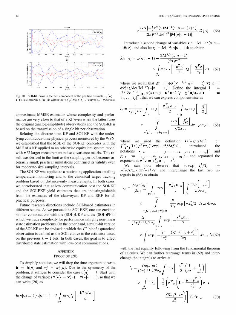
The results of simulating this setup are depicted in Figs. 8and 9, where we see that the SOI-KF succeeds in tracking thetarget with distance error for the position estimates of less than10 m. Similar conclusions can be obtained from Fig. 10 thatdepicts the error in the first coordinate com-pared with the curves for the SOI-KF and theKF. As expected, the SOI-KF error matches the KF error withboth of them within the corresponding curves.While this accuracy is just a result of the specific parameters ofthe experiment, the important point here is that the clairvoyantEKF and the SOI-EKF yield almost identical performance evenwhen the former relies on analog-amplitude observations andthe SOI-EKF on the transmission of a single bit per sensor.

VII. CONCLUDING REMARKS

Relying on the SOI, we considered the problem of distributedstate estimation in the context of wireless sensor networks.The binary SOI data render the problem nonlinear and lead toprohibitively complex MMSE state estimation. This motivatedan approximation leading to the SOI-KF which constitutes an


Fig. 10. SOI-KF error in the first component of the position estimate x (n)�x̂ (njn) (error in x (n)) is within the�3 [M(njn)] curves (3�� curves).

approximate MMSE estimator whose complexity and perfor-mance are very close to that of a KF even when the latter fusesthe original (analog-amplitude) observations and the SOI-KF isbased on the transmission of a single bit per observation.

Relating the discrete-time KF and SOI-KF with the under-lying continuous-time physical process monitored by the WSN,we established that the MSE of the SOI-KF coincides with theMSE of a KF applied to an otherwise equivalent system modelwith larger measurement noise covariance matrix. This re-sult was derived in the limit as the sampling period becomes ar-bitrarily small; practical simulations confirmed its validity evenfor moderate-size sampling intervals.

The SOI-KF was applied to a motivating application entailingtemperature monitoring and to the canonical target trackingproblem based on distance-only measurements. In both cases,we corroborated that at low communication cost the SOI-KFand the SOI-EKF yield estimates that are indistinguishablefrom the estimates of the clairvoyant KF and EKF for allpractical purposes.

Future research directions include SOI-based estimators indifferent setups. As we pursued the SOI-EKF, one can envisionsimilar combinations with the (SOI-)UKF and the (SOI-)PF inwhich we trade complexity for performance in highly non-linearstate estimation problems. On the other hand, a multi-bit versionof the SOI-KF can be devised in which the bit of a quantizedobservation is defined as the SOI relative to the estimator basedon the previous bits. In both cases, the goal is to effectdistributed state estimation with low-cost communications.

APPENDIX

PROOF OF (20)

To simplify notation, we will drop the time argument to writeand . Due to the symmetry of the

problem, it suffices to consider the case . Start withthe change of variables , so that wecan write (26) as

(66)

Introduce a second change of variables, and also let to obtain

(67)

where we recall that. Define the integral

, that we can express componentwise as

(68)

where we used the definition, introduced the

notations and, and separated the

exponent as .We can now observe that

and interchange the last two in-tegrals in (68) to obtain

(69)

with the last equality following from the fundamental theoremof calculus. We can further rearrange terms in (69) and inter-change the integrals to arrive at

(70)


Consider now the quadratic form in the exponent of the secondintegral, and let us summarize a number of properties about thisform in the following lemma.

Lemma 1: If we define the matrix ,it holds that:

a) the inverse of is given by ;b) the determinant of is ;c) the quadratic form in the exponent of the second integral

in (70) can be written as

(71)

with .Proof: Statement a) follows from the matrix inversion

lemma, and can also be proved by verifying that . Toprove b), let be an eigenvector of ; being an eigenvectorof , must satisfy

(72)

for some constant . Note that (72) is satisfied bywith , and by any perpendicular to

such that with . Since the determinantcan be expressed as the product of the eigenvalues, we have

(73)

However, the dimension of the subspace perpendicular tois , and thus, . Statement b) is obtained bysimply rearranging terms.

To prove c), expand the right-hand side and verify that theequality is indeed true.

Using Lemma 1-c), we can rewrite (70) as

(74)

where the two integrals are independent. The second integral isthe integral of a -dimensional Gaussian distribution over

which regardless of is equal to ;given that is given by the inverse of the expression inLemma 1-b), we obtain

(75)

The first integral in (74) is the integral of a Gaussian bell overand is thus given by times the standard deviation

(76)

Substituting (75) and (76) into (74), we obtain

(77)

Placing the components of given by (77) into (67) yields theexpression

(78)

Recalling that , (26) follows for .For , the opposite result follows from symmetry.

REFERENCES

[1] J. Aslam, Z. Butler, F. Constantin, V. Crespi, G. Cybenko, and D. Rus,“Tracking a moving object with a binary sensor network,” in Proc. 1stInt. Conf. Embedded Networked Sensor Systems, Los Angeles, CA,2003, pp. 150–161.

[2] Y. Bar-Shalom and X. Li, Estimation and Tracking: Principles, Tech-niques, and Software. Norwood, MA: Artech House, 1993.

[3] B. Beferull-Lozano, R. L. Konsbruck, and M. Vetterli, “Rate-distor-tion problem for physics based distributed sensing,” in Proc. Int. Conf.Acoustics, Speech, and Signal Processing, Montreal, QC, Canada, May2004, vol. 3, pp. 913–916.

[4] D. Blatt and A. Hero, “Distributed maximum likelihood estimation forsensor networks,” in Proc. Int. Conf. Acoustics, Speech, and Signal Pro-cessing, Montreal, QC, Canada, May 2004, vol. 3, pp. 929–932.

[5] C. Chong, S. Mori, and K. Chang, Distributed Multitarget MultisensorTracking. Norwood, MA: Artech House, 1990.

[6] R. Curry, W. Vandervelde, and J. Potter, “Nonlinear estimation withquantized measurements—PCM, predictive quantization, and datacompression,” IEEE Trans. Inf. Theory, vol. IT-16, no. 3, pp. 152–161,March 1970.

[7] P. Djuric, J. Kotecha, J. Zhang, Y. Huang, T. Ghirmai, M. Bugallo, andJ. Miguez, “Particle filtering,” IEEE Signal Process. Mag, vol. 20, no.9, pp. 19–38, Sep. 2003.

[8] P. Djuric, M. Vemula, and M. Bugallo, “Tracking with particle filteringin tertiary wireless sensor networks,” in Proc. Int. Conf. Acoustics,Speech and Signal Processing, Philadelphia, PA, Mar. 19–23, 2005,vol. 4, pp. 757–760.

[9] E. Ertin, R. Moses, and L. Potter, “Network parameter estimation withdetection failures,” in Proc. Int. Conf. Acoustics, Speech, and SignalProcessing, Montreal, QC, Canada, May 2004, vol. 2, pp. 273–276.

[10] J. Gubner, “Distributed estimation and quantization,” IEEE Trans. Inf.Theory, vol. 39, no. 4, pp. 1456–1459, Jul. 1993.

[11] V. Gupta, T. Chung, B. Hassibi, and R. M. Murray, “On a stochasticsensor selection algorithm with applications in sensor scheduling anddynamic sensor coverage,” Automatica, vol. 42, no. 2, pp. 251–260,Feb. 2006.

[12] F. Gustafsson, F. Gunnarsson, N. Bergman, U. Forssell, J. Jansson, R.Karlsson, and P.-J. Nordlund, “Particle filters for positioning, naviga-tion, and tracking,” IEEE Trans. Signal Process., vol. 50, no. 2, pp.425–437, Feb. 2002.

[13] A. Jadbabaie, J. Lin, and A. Morse, “Coordination of groups of mobileautonomous agents using nearest neighbor rules,” IEEE Trans. Autom.Control, vol. 48, no. 6, pp. 988–1001, Jun. 2003.

[14] S. Julier and J. Uhlmann, “Unscented filtering and nonlinear estima-tion,” Proc. IEEE, vol. 92, no. 3, pp. 401–422, Mar. 2004.

[15] S. M. Kay, Fundamentals of Statistical Signal Processing—EstimationTheory. Upper Saddle River, NJ: Prentice-Hall, 1993.

[16] J. Kotecha and P. Djuric, “Gaussian particle filtering,” IEEE Trans.Signal Process., vol. 51, no. 10, pp. 2602–2612, Oct. 2003.


[17] W. Lam and A. Reibman, “Quantizer design for decentralized systemswith communication constraints,” IEEE Trans. Commun., vol. 41, no.8, pp. 1602–1605, Aug. 1993.

[18] Z.-Q. Luo, “An isotropic universal decentralized estimation scheme fora bandwidth constrained ad hoc sensor network,” IEEE J. Select. AreasCommun., vol. 23, no. 4, pp. 735–744, April 2005.

[19] A. Mainwaring, D. Culler, J. Polastre, R. Szewczyk, and J. Anderson,“Wireless sensor networks for habitat monitoring,” in Proc. 1st ACMInt. Workshop on Wireless Sensor Networks and Applications, Atlanta,GA, 2002, vol. 3, pp. 88–97.

[20] P. S. Maybeck, Stochastic Models, Estimation and Control—Vol. 1, 1sted. New York: Academic, 1979.

[21] A. I. Mourikis and S. I. Roumeliotis, “Optimal sensor scheduling forresource-constrained localization of mobile robot formations,” IEEETrans. Robotics, vol. 22, no. 5, pp. 917–931, Oct. 2006.

[22] H. Papadopoulos, G. Wornell, and A. Oppenheim, “Sequential signalencoding from noisy measurements using quantizers with dynamic biascontrol,” IEEE Trans. Inf. Theory, vol. 47, no. 3, pp. 978–1002, Mar.2001.

[23] S. S. Pradhan, J. Kusuma, and K. Ramchandran, “Distributed compres-sion in a dense microsensor network,” IEEE Signal Process. Magazine,vol. 19, no. 3, pp. 51–60, Mar. 2002.

[24] M. G. Rabbat and R. D. Nowak, “Decentralized source localization andtracking,” in Proc. Int. Conf. Acoustics, Speech, and Signal Processing,Montreal, QC, Canada, May 2004, vol. 3, pp. 921–924.

[25] A. Ribeiro and G. B. Giannakis, “Bandwidth-constrained distributedestimation for wireless sensor networks, part II: unknown pdf,” IEEETrans. Signal Process., vol. 54, no. 7, pp. 2784–2796, Jul. 2006.

[26] ——, “Bandwidth-constrained distributed estimation for wirelesssensor networks, Part I: Gaussian case,” IEEE Trans. Signal Process.,vol. 54, no. 3, pp. 1131–1143, Mar. 2006.

[27] A. Ribeiro, G. B. Giannakis, and S. I. Roumeliotis, “SOI-KF: dis-tributed Kalman filtering with low-cost communications using thesign of innovations,” in Proc. Int. Conf. Acoustics, Speech, SignalProcessing, Toulouse, France, May 14–19, 2006, pp. IV-153–IV-156.

[28] A. H. Sayed, Fundamentals of Adaptive Filtering, 1st ed. New York:Wiley-Interscience, 2003.

[29] D. Williamson, “Finite wordlength design of digital Kalman filters forstate estimation,” IEEE Trans. Autom. Control, vol. AC-30, no. 10, pp.930–939, Oct. 1985.

Alejandro Ribeiro (S’02) received the B.Sc. degreein electrical engineering from the Universidad dela Republica Oriental del Uruguay, Montevideo,Uruguay, in 1998. Since May 2003, he has beenworking towards the Ph.D. degree in the Departmentof Electrical and Computer Engineering, Universityof Minnesota, Minneapolis, where he received theM.Sc. degree in electrical engineering in 2005.

From 1998 to 2003, he was a member of the Tech-nical Staff at Bellsouth Montevideo. His researchinterests lie in the areas of communication theory,

signal processing, and networking. His current research focuses on wirelesscooperative communications, random access, wireless ad hoc and sensornetworks, and distributed signal processing.

Mr. Ribeiro is a Fulbright Scholar.

Georgios B. Giannakis (F’97) received the Diplomain electrical engineering from the National TechnicalUniversity of Athens, Athens, Greece, 1981. FromSeptember 1982 to July 1986, he was with the Uni-versity of Southern California (USC), where he re-ceived the M.Sc. degree in electrical engineering in1983, the M.Sc. degree in mathematics in 1986, andthe Ph.D. degree in electrical engineering in 1986.

After lecturing for one year at USC, he joinedthe University of Virginia, Charlottesville, in 1987,where he became a Professor of Electrical Engi-

neering in 1997. Since 1999, he has been a Professor with the Department ofElectrical and Computer Engineering at the University of Minnesota, Min-neapolis, where he now holds an ADC Chair in Wireless Telecommunications.His general interests span the areas of communications and signal processing,estimation and detection theory, time-series analysis, and system identifi-cation—subjects on which he has published more than 250 journal papers,400 conference papers, and two edited books. Current research focuses ondiversity techniques for fading channels, complex-field and space-time coding,multicarrier, ultra-wide band wireless communication systems, cross-layerdesigns, and sensor networks.

Dr. Giannakis is the (co-) recipient of six paper awards from the IEEE SignalProcessing (SP) and Communications Societies (1992, 1998, 2000, 2001, 2003,and 2004). He also received Technical Achievement Awards from the SP Societyin 2000 and from EURASIP in 2005. He served as Editor in Chief for the IEEESIGNAL PROCESSING LETTERS, as Associate Editor for the IEEE TRANSACTIONS

ON SIGNAL PROCESSING and the IEEE SIGNAL PROCESSING LETTERS, as Secre-tary of the SP Conference Board, as member of the SP Publications Board, as amember and Vice-Chair of the Statistical Signal and Array Processing TechnicalCommittee, as Chair of the SP for Communications Technical Committee, andas a member of the IEEE Fellows Election Committee. He has also served asa member of the IEEE-SP Society’s Board of Governors, the Editorial Boardfor the PROCEEDINGS OF THE IEEE and the steering committee of the IEEETRANSACTIONS ON WIRELESS COMMUNICATIONS.

Stergios I. Roumeliotis (M’00) received theDiploma in electrical engineering from the NationalTechnical University of Athens, Athens, Greece, in1995, and the M.S. and Ph.D. degrees in electricalengineering from the University of Southern Cali-fornia, Los Angeles, in 1999 and 2000, respectively.

From 2000 to 2002, he was a Postdoctoral Fellowat the California Institute of Technology, Pasadena.Since 2002, he has been an Assistant Professor in theDepartment of Computer Science and Engineeringat the University of Minnesota, Minneapolis. His re-

search interests include inertial navigation of aerial and ground autonomousvehicles, fault detection and identification, and sensor networks. Recently, hisresearch has focused on distributed estimation under communication and pro-cessing constraints and active sensing for reconfigurable networks of mobilesensors.

Dr. Roumeliotis is the recipient of the McKnight Land-Grant ProfessorshipAward and the NASA Tech Briefs Award.

Documents

IEEE TRANSACTIONS ON SIGNAL PROCESSING 1 SOI …stergios/papers/TSP06-SOI-KF.pdf · IEEE TRANSACTIONS ON SIGNAL PROCESSING 1 SOI-KF: Distributed Kalman Filtering With Low-Cost Communications