IEEE TRANSACTIONS ON CIRCUITS AND SYSTEMS FOR VIDEO TECHNOLOGY 1

Abstract— In this paper, a new heat-map-based (HMB)

algorithm is proposed for group activity recognition. The

proposed algorithm first models human trajectories as series of

“heat sources” and then applies a thermal diffusion process to

create a heat map (HM) for representing the group activities.

Based on this heat map, a new key-point based (KPB) method is

used for handling the alignments among heat maps with different

scales and rotations. And a surface-fitting (SF) method is also

proposed for recognizing group activities. Our proposed HM

feature can efficiently embed the temporal motion information of

the group activities while the proposed KPB and SF methods can

effectively utilize the characteristics of the heat map for activity

recognition. Experimental results demonstrate the effectiveness of

our proposed algorithms.

I. INTRODUCTION

etecting group activities or human interactions has

attracted increasing research interests in many

applications such as video surveillance and

human-computer interaction [1-6].

Many algorithms have been proposed for recognizing group

activities or interactions [1-6, 24-25]. Zhou et al. [2] propose to

detect pair-activities by extracting the causality, mean, variance

features from bi-trajectories. Ni et al. [3] further extend the

causality features into three types of individuals, pairs and

groups. Besides, Chen et al. [5] detect group activities by

introducing the connected active segmentations for

representing the connectivity among people. Cheng et al. [4]

propose the Group Activity Pattern for representing group

activities as Gaussian processes and extract Gaussian

parameters as features. However, most of the existing

algorithms extract the overall features from the activities’ entire

motion information (e.g., the statistical average of the motion

trajectory). These features cannot suitably embed activities’

temporal motion information (e.g., fail to indicate where a

This work was supported in part by the National Science Foundation of

China grants (61001146 and 61202154), the Open Project Program of the

National Laboratory of Pattern Recognition (NLPR), the SMC grant of SJTU, Shanghai Pujiang Program (12PJ1404300), and the Chinese national 973 grants

(2010CB731401). The basic idea of this paper appeared in our conference version [27]. In this

version, we propose new KPB and SF methods to handle the heat map

alignments, carry out detailed analysis, and present more performance results. The first two authors contributed equally to this paper.

H. Chu and W. Lin are with the Department of Electronic Engineering, Shanghai Jiao Tong University, Shanghai 200240, China (email: {chuhang321,

wylin}@sjtu.edu.cn).

J. Wu is with the School of Computer Engineering, Nanyang Technological University, Singapore (email: jxwu@ntu.edu.sg).

B. Sheng is with the Department of Computer Science, Shanghai Jiao Tong University, Shanghai 200240, China (email: shengbin@cs.sjtu.edu.cn).

Z. Chen is with MediaTek Inc., USA (zzchen@ieee.org).

Copyright (c) 2013 IEEE. Personal use of this material is permitted. However, permission to use this material

for any other purposes must be obtained from the IEEE by sending an email to pubs-permissions@ieee.org.

person is in the video at a certain moment). Thus, they will have

limitations when recognizing more complex group activities.

Although some methods [6, 29] incorporate the temporal

information with chain models such as the Hidden Markov

Models (HMM), they have the disadvantage of requiring

large-scale training data [17]. Besides, other methods try to

include the temporal information by attaching time stamps with

trajectories and perform recognition by associating these time

stamp labels [18-19]. However, these methods are more

suitable for scenarios with only one trajectory or trajectories

with fixed correspondence. They will become less effective or

even infeasible when describing and differentiating the

complicated temporal interactions among multiple trajectories

in group activities. Furthermore, [24] and [25] give more

extensive survey about the existing techniques used in group

activity recognition and crowd analysis.

In another part, handling motion uncertainties is also an

important issue in group activity recognition. Since the motions

of people vary inherently in group activities, the recognition

accuracy may be greatly affected by this uncertain motion

nature. Although some methods utilize Gaussian processes

estimation or filtering to handle this uncertain problem [3, 4],

they do not simultaneously consider the issue for reserving the

activities’ temporal motion information.

Furthermore, the recognition method is a third key issue for

recognizing group activities. Although the popularly-used

models such as Linear Discriminative Analysis and HMM [6]

show good results in many scenarios, their training difficulty

and the requirement of the training data scale will increase

substantially when the feature vector length becomes large or

the group activity becomes complex. Therefore, it is also

non-trivial to develop more flexible recognition methods for

effectively handling the recognition task.

In this paper, we propose a new heat-map-based (HMB)

algorithm for group activity recognition. The contributions of

our work can be summarized as follows:

(1) We propose a new heat map (HM) feature to represent

group activities. The proposed HM can effectively catch

the temporal motion information of the group activities.

(2) We propose to introduce a thermal diffusion process to

create the heat map. By this way, the motion uncertainty

from different people can be efficiently addressed.

(3) We propose a key-point based (KPB) method to handle the

alignments among heat maps with different scales and

rotations. By this way, the heat map differences due to

motion uncertainty can be further reduced and the

follow-up recognition process can be greatly facilitated.

(4) We also propose a new surface-fitting (SF) method to

recognize the group activities. The proposed SF method

can effectively catch the characteristics of our heat map

feature and perform recognition efficiently.

The remainder of this paper is organized as follows. Section

Hang Chu, Weiyao Lin, Jianxin Wu, Bin Sheng, and Zhenzhong Chen

A Heat-Map-based Algorithm for Recognizing Group

Activities in Videos

D

IEEE TRANSACTIONS ON CIRCUITS AND SYSTEMS FOR VIDEO TECHNOLOGY 2

II describes the basic ideas of our proposed HM feature as well

as the KPB and SF methods. Section III presents the details of

our HMB algorithm. The experimental results are shown in

Section IV and Section V concludes the paper.

II. BASIC IDEAS

A. The heat-map features

As mentioned, given the activities’ motion information

(i.e., motion trajectory in this paper), directly extracting the

global features will lose the useful temporal information. In

order to avoid such information loss, we propose to model the

activity trajectory as a series of heat sources. As shown in

Figure 1, (a) is the trajectory of one person. In order to transfer

the trajectories into heat source series, we first divide the entire

video scene into small non-overlapping patches (i.e., the small

squares in (b)). If the trajectory goes through a patch, this patch

will be defined as one heat source. By this way, a trajectory can

be transferred into a series of heat sources, as in Figure 1 (b).

Furthermore, in order to further catch the temporal information

of the trajectory, we also introduce a decay factor on different

heat sources such that the thermal energies of the “older” heat

sources (i.e., patches closer to the stating point of the trajectory)

are smaller while the “newer” heat sources will have larger

thermal energies. By this way, the thermal values of the heat

source series can be arranged increasingly according to the

direction of the trajectory and the temporal information can be

effectively embedded.

(a) (b)

(c) (d)

Figure 1. (a): The activity trajectory; (b) The corresponding heat source series;

(c) The heat map (HM) diffused from the heat source series in (b); (d) The HM surface of (c) in 3D.

Furthermore, since people’s trajectories may have large

variations, directly using the heat source series as features will

be greatly affected by this motion fluctuation. Therefore, in

order to reduce the motion fluctuation, we further propose to

introduce a thermal diffusion process to diffuse the heats from

the heat source series to the entire scene. We call this diffusion

result as the heat map (HM). With our HM feature, we can

describe the activities’ motion information by 3D surfaces.

Figure 1 (c) and (d) show the HM of the trajectory in Figure 1 (a)

in 2D format and in 3D surface format, respectively. Several

points need to be mentioned about the HM in our paper:

(1) Note that although the heat diffusion was introduced in

object segmentation in some works [8], the mechanism and

utilization of HM in our algorithm is far different from

them. And to the best of our knowledge, this is the first

work to introduce HM into group activity recognition.

(2) The definition of “heat map” in this paper is also different

from the ones used in some activity recognition methods

[11-12]. In those methods [11-12], the heat maps are

defined to reflect the number of translations among

different regions without considering the order during

passes. Thus, they are more focused on reflecting the

“popularity” of regions (i.e., whether some regions are

more often visited by people) while neglecting the

temporal motion information as well as the interactions

among trajectories.

(3) With the HM features, we can perform offline activity

recognition by creating HMs for the entire trajectories.

This off-line recognition is important in many applications

such as video retrieval and surveillance video investigation

[6, 15]. Furthermore, the HM features can also be used to

perform on-line (or on-the-fly) recognition by using

shorter sliding windows. This point will be further

discussed in the experimental result section.

After the calculation of HM features, we can use them for

recognizing group activities. However, two problems need to

be solved for perform recognition with HM features. They are

described in the following.

B. The alignments among heat maps

Although the thermal diffusion process can reduce the

motion fluctuation effect due to motion uncertainty or tracking

biases, the resulting HM will still differ a lot due to the various

motion patterns for different activities. For example, in Figure 2

(a), since the trajectories of human activities take varies

directions and lengths, the heat maps for the same type of group

activity show large differences in scales and rotations.

Therefore, alignments are necessary to reduce these HM

differences for facilitating the follow-up recognition process.

In this paper, we propose a new key-point based (KPB)

method to handle the alignments among heat maps. Since our

heat maps are featured with peaks (i.e., local maxima in HM as

in Figure 1 (d)), the proposed KPB method extracts the peaks

from HMs as the key points and then performs alignments

according to these key points in an iterative way. By this way,

the scale and rotation variations among heat maps can be

effectively removed. Figure 2 (b) shows the alignment results

of the heat maps in (a) by our KPB method. More details about

the KPB method will be described in the next section.

(a) Heat maps for the group activity “gather” performed by different people.

(b) The alignment results of the heat maps in (a) by our KPB method.

Figure 2. The alignments among heat maps.

IEEE TRANSACTIONS ON CIRCUITS AND SYSTEMS FOR VIDEO TECHNOLOGY 3

C. Recognition based on the heat maps

Since the HM feature includes rich information, the

problem then comes to the selection of a suitable method for

performing recognition based on this HM feature. In this paper,

we further propose a surface-fitting (SF) method for activity

recognition. In our SF method, a set of standard surfaces are

first identified for representing different activities. Then, the

similarities between the surface of the input HM and the

standard surfaces are calculated. And finally, the best matched

standard surface will be picked up and its corresponding

activity will become the recognized activity for the input HM.

The process of our SF method is shown in Figure 3.

With the basic ideas of the HM feature, the KPB and the SF

methods described above, we can propose our heat-map-based

(HMB) group activity recognition algorithm. It is described in

detail in the following section.

Figure 3. The process of the surface-fitting (SF) method.

III. THE HMB ALGORITHM

The framework of our HMB algorithm can be described by

Figure 4. In Figure 4, the input group activities’ trajectories are

first transferred into heat source series, then the thermal

diffusion process is performed to create the HM feature for

describing the input group activity. After that, the KPB method

is used for aligning HMs and finally the SF method is used for

recognizing the group activities. As mentioned, the heat source

series transfer, the thermal diffusion, the KPB method, and the

SF method are the four major contributions of our proposed

algorithm. Thus, we will focus on describing these four parts in

the following.

HM feature creation

Activity Recognition

Group activity trajectories

Transfer into heat source series

Diffuse to create heat map

Heat Map Alignment

Recognition result

Recognize group activities by

the surface-fitting method

Figure 4. The process of the HMB algorithm.

A. Heat source series transfer

Assume that we have in total j trajectories in the current

group activity. The thermal energy Ei of the heat source patch i

can be calculated by:

j

ttk

ji,ijid,curteEE (1)

where jid,curt ttk

e

is the time decay term [10], kt is the

temporal decay coefficient, tcur is the current frame number, and

tid,j is the frame number when the j-th trajectory leaves patch i.

ji,E is the accumulated thermal energy for trajectory j in patch

i and it can be calculated by Eq. (2). From Eq. (1), we can see

that “newer” heat sources of the trajectory have more thermal

energies than the “older” heat sources.

j,isj,id

j,isj,idtttt

0

)tt(k

t

tk

j,i e1k

CdteCE (2)

where tis,j and tid,j are the frame number when the j-th trajectory

enters and leaves patch i, respectively. kt is the temporal decay

coefficient as in Eq. (1), and C is a constant. In the experiments

of our paper, C is set to be 1. From Eq. (2), we can see that the

accumulated thermal energy is proportional to the stay length of

trajectory j at patch i. If j stays in i for longer time, more thermal

energy will be accumulated in patch i. On the other hand, if no

trajectory goes through patch i, the accumulated thermal energy

of patch i will be 0, indicating that patch i is not a heat source

patch.

B. Thermal diffusion

After getting the heat source series by Eq. (1), the thermal

diffusion process will be performed over the entire scene to

create the HM. The HM value Hi at patch i after diffusion [10]

can be calculated by:

N

eEH

N

1

,k

l

i

l

lid p

(3)

where El is the thermal energy of the heat source patch l, N is

the total number of heat source patches. kp is the spatial

diffusion coefficient, and d(i, l) is the distance between patches

i and l.

The advantage of the thermal diffusion process can be

described by Figure 5. In Figure 5, the left column lists two

different trajectory sets for the group activity “gather”. Due to

the variation of human activity or tracking biases, these two

trajectory sets are obviously different from each other. And

these differences are exactly transferred to their heat source

series (the middle column). However, with the thermal

diffusion process, the trajectory differences are suitably

“blurred”, which makes their HMs (the right column) close to

each other. At the same time, the temporal information of the

two group activities is still effectively reserved in the HMs.

Also, Figure 6 shows the example HM surfaces for different

group activities defined in Table 1. From Figure 6, it is clear

that our proposed HM can precisely catch the activities’

temporal information and show obviously distinguishable

patterns among different activities.

IEEE TRANSACTIONS ON CIRCUITS AND SYSTEMS FOR VIDEO TECHNOLOGY 4

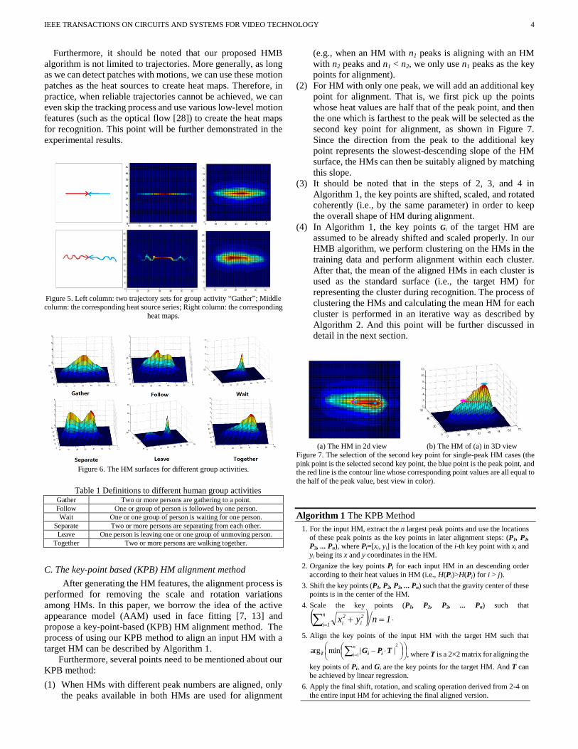
Furthermore, it should be noted that our proposed HMB

algorithm is not limited to trajectories. More generally, as long

as we can detect patches with motions, we can use these motion

patches as the heat sources to create heat maps. Therefore, in

practice, when reliable trajectories cannot be achieved, we can

even skip the tracking process and use various low-level motion

features (such as the optical flow [28]) to create the heat maps

for recognition. This point will be further demonstrated in the

experimental results.

Figure 5. Left column: two trajectory sets for group activity “Gather”; Middle column: the corresponding heat source series; Right column: the corresponding

heat maps.

Figure 6. The HM surfaces for different group activities.

Table 1 Definitions to different human group activities Gather Two or more persons are gathering to a point.

Follow One or group of person is followed by one person.

Wait One or one group of person is waiting for one person.

Separate Two or more persons are separating from each other.

Leave One person is leaving one or one group of unmoving person.

Together Two or more persons are walking together.

C. The key-point based (KPB) HM alignment method

After generating the HM features, the alignment process is

performed for removing the scale and rotation variations

among HMs. In this paper, we borrow the idea of the active

appearance model (AAM) used in face fitting [7, 13] and

propose a key-point-based (KPB) HM alignment method. The

process of using our KPB method to align an input HM with a

target HM can be described by Algorithm 1.

Furthermore, several points need to be mentioned about our

KPB method:

(1) When HMs with different peak numbers are aligned, only

the peaks available in both HMs are used for alignment

(e.g., when an HM with n1 peaks is aligning with an HM

with n2 peaks and n1 < n2, we only use n1 peaks as the key

points for alignment).

(2) For HM with only one peak, we will add an additional key

point for alignment. That is, we first pick up the points

whose heat values are half that of the peak point, and then

the one which is farthest to the peak will be selected as the

second key point for alignment, as shown in Figure 7.

Since the direction from the peak to the additional key

point represents the slowest-descending slope of the HM

surface, the HMs can then be suitably aligned by matching

this slope.

(3) It should be noted that in the steps of 2, 3, and 4 in

Algorithm 1, the key points are shifted, scaled, and rotated

coherently (i.e., by the same parameter) in order to keep

the overall shape of HM during alignment.

(4) In Algorithm 1, the key points Gi of the target HM are

assumed to be already shifted and scaled properly. In our

HMB algorithm, we perform clustering on the HMs in the

training data and perform alignment within each cluster.

After that, the mean of the aligned HMs in each cluster is

used as the standard surface (i.e., the target HM) for

representing the cluster during recognition. The process of

clustering the HMs and calculating the mean HM for each

cluster is performed in an iterative way as described by

Algorithm 2. And this point will be further discussed in

detail in the next section.

(a) The HM in 2d view (b) The HM of (a) in 3D view

Figure 7. The selection of the second key point for single-peak HM cases (the

pink point is the selected second key point, the blue point is the peak point, and the red line is the contour line whose corresponding point values are all equal to

the half of the peak value, best view in color).

Algorithm 1 The KPB Method

1. For the input HM, extract the n largest peak points and use the locations

of these peak points as the key points in later alignment steps: (P1, P2,

P3, ... Pn), where Pi=[xi, yi] is the location of the i-th key point with xi and

yi being its x and y coordinates in the HM.

2. Organize the key points Pi for each input HM in an descending order according to their heat values in HM (i.e., H(Pi)>H(Pj) for i > j).

3. Shift the key points (P1, P2, P3, ... Pn) such that the gravity center of these points is in the center of the HM.

4. Scale the key points (P1, P2, P3, ... Pn) such that

1nyxn

1i

2

i

2

i .

5. Align the key points of the input HM with the target HM such that

2

1||minarg

n

iTPG iiT , where T is a 2×2 matrix for aligning the

key points of Pi, and Gi are the key points for the target HM. And T can

be achieved by linear regression.

6. Apply the final shift, rotation, and scaling operation derived from 2-4 on

the entire input HM for achieving the final aligned version.

IEEE TRANSACTIONS ON CIRCUITS AND SYSTEMS FOR VIDEO TECHNOLOGY 5

Algorithm 2 Clustering the HMs and calculating the mean HM

key points for each cluster in the training set

1. Cluster the HMs in the training set according to their activity labels.

2. for each HM v in the training set do

3. Shift the key points (P1,v, P2,v, P3,v, ... Pn,v) of HM v such that the

gravity center of these point is in the center of the HM.

4. Scale the key points (P1,v, P2,v, P3,v, ... Pn,v) of HM v such that

1nyxn

1i

2

vi,

2

vi, .

5. end for

6. for each cluster u do

7. Randomly select an HM in cluster u as the initial mean HM and

define the key points for this mean HM as (G1u, G2

u, G3u, ... Gn

u)

8. for each HM v in cluster u do

9. Scale the key points (P1,v, P2,v, P3,v, ... Pn,v) of HM v such that

1nyxn

1i

2

vi,

2

vi, .

10. Align the key points of the HM v with the current mean HM

such that

2

1||minarg

n

i vvi,

u

iT TPGv , where Tv is the

alignment matrix for v.

11. Move the key points of the HM v to the aligned places, i.e.,

vvi,, TPP new

vi.

12. end for

13. Update the key points of the mean HM of cluster u by:

NUMNUM

v/

1

new

vi

new ,

u,

i PG , where NUM is the number of HMs

in cluster u.

14. If not converged and iteration time≤ 1000, return to 8.

15. Align all the HMs in cluster u to the calculated key points of the

mean HM. And the final mean HM can be achieved by averaging or

selecting the most fitted one among these aligned HMs.

16. end for

D. The surface-fitting (SF) method for activity recognition

With the HM feature and the KPB alignment method, we can

then perform recognition based on our surface-fitting (SF)

method. The surface-fitting process can be described by Eq.

(4):

||||minminargm m

*

m

SD,mHMTm

SST (4)

where m* is the final recognized activity. SHM is the HM surface

of the input activity, SSD,m is the standard surface for activity m.

Tm is the alignment operator derived by Algorithm 1 for

aligning with SSD,m. And || · || is the absolute difference between

two HM surfaces. From Eq. (4), we can see that the SF method

includes two steps. In the first step, the input HM is aligned to

fit with each standard surface. And then in the second step, the

standard surface that best fits the input HM surface will be

selected as the recognized activity.

As shown in Algorithm 2, the standard surface can be

achieved by clustering the training HMs and taking the mean

HM for each cluster. However, since the HMs may still vary

within the same activity, it may still be less effective to use one

fixed HM as the standard surface for recognition. Therefore, in

this paper, we further propose an adaptive surface-fitting (ASF)

method which selects the standard surface in an adaptive way.

The proposed ASF method can be described by Eq. (5).

HMtrSS

mHMtrTm

SSTwmtr, N

tr,

* minGAmaxargm (5)

where SHM is the HM surface for the input activity. Str,m is the

HM surface for activity m in the training data. Ttr is the

alignment operator for aligning with Str. Nw(SHM) is set

containing the w most similar HM surfaces to SHM. GA(·) is the

Gaussian kernel function as defined by Eq. (6).

)2

||exp()(GA

2

2

xx (6)

where σ controls the steepness of the kernel.

From Eq. (5), we can see that the proposed ASF method

adaptively select the most similar HM surfaces as the standard

surfaces for recognition. By this way, the in-class HM surface

variation effect can be effectively reduced. Furthermore, by

introducing the Gaussian kernel, different training surfaces Str,m

can be allocated different importance weights according to their

similarity to the input HM SHM during the recognition process.

Furthermore, several things need to be mentioned about the

ASF method:

(1) When w>1 in Nw,m(SHM), the ASF method can be viewed as

an extended version of the k-nearest-neighbor (KNN)

methods [14] where the kernel-weighted distance between

points is calculated by the absolution difference between

the aligned HM surfaces.

(2) When w=1 in Nw,m(SHM), the ASF method is simplified to

finding a Str,m in the training set that can best represent the

input SHM.

IV. EXPERIMENTAL RESULTS

In this section, we show experimental results for our

proposed HMB algorithm. The ASF method is used for

recognition in our experiments. And the patch size is set to be

10×10 based on our experimental statistics, in order to achieve

satisfactory resolution of the HM surface while maintaining the

efficiency of computation. Furthermore, for each input video

clip, the heat map is created for the entire clip.

A. Experimental results on the BEHAVE dataset

In this sub-section, we perform five different sets of

experiments on the BEHAVE dataset to evaluate our proposed

algorithm.

First of all, we change the values of the temporal decay

parameter kt and the thermal diffusion parameter kp in Eqs (1)

and (3) to see their effects in recognition performances. We

select 200 video clips from the BEHAVE dataset [1] and

recognize six group activities defined in Table 1. The sample

number for each group activity is shown in Table 2. Each video

clip includes 2-5 trajectories. In order to exam the algorithm’s

performance against tracking fluctuation and tracking biases,

we perform 5 rounds of experiments where in each round,

different fluctuation and biases effects are added on the

ground-truth trajectories. The final results are averaged over the

five rounds. The recognition results under 75%-training and

25%-testing are shown in Tables 3 and 4.

IEEE TRANSACTIONS ON CIRCUITS AND SYSTEMS FOR VIDEO TECHNOLOGY 6

Table 2 The sample number for different group activities for the

experiments in Tables 3-4 and Figures 8-9 Gather Follow Wait Separate Leave Together Total

33 33 34 33 33 34 200

Table 3 The TER rates of HMB algorithm under different spatial

diffusion coefficient kp values (when kt =0.125) kp=0.1 kp =1 kp =2 kp =3 kp =4 kp =5 kp =∞

HMB (w=1) 42% 16% 13% 15% 17% 19% 38%

Table 4 TER rates of HMB algorithm under different temporal

diffusion coefficient kt values (when kp =2) kt=0.025 kt =0.125 kt =0.25 kt =0.5 kt =1 kt =∞

HMB (w=1) 25% 13% 15% 17% 20% 45%

Tables 3-4 show the total error rate (TER) rate for different kt

and kp values. The TER rate is calculated by Nt_miss/Nt_f where

Nt_miss is the total number of misdetection activities for both

normal and abnormal activities and Nt_f is the total number of

activity sequences in the test set [6, 15]. TER reflects the

overall performance of the algorithm in recognizing all activity

types [6, 15]. In Tables 3-4, our HMB algorithm is performed

where w in Eq. (5) is set to be 1 (i.e., selecting only the most

similar HM surface in the training set during recognition).

Furthermore, the example HM surfaces under different kt and kp

values are shown in Figures 8 and 10, respectively.

(a) kp=0.0001 (b) kp=0.25 (c) kp=1000

Figure 8. Example HM surfaces for activity “together” with different kp values.

(a) kt=0 (b) kt=0.03 (c) kt=1000

Figure 9. Example HM surfaces for activity “together” with different kt values.

From Table 3 and Figure 8, we can see that: (1) When kp is

set to be a very small number (such as Figure 8 (a)), the thermal

diffusion effect is too strong that the HM is close to a flat

surface. In this case, the effectiveness of the HM cannot fully

work and the recognition performances will be decreased. (2)

On the contrary, if kp is set to be extremely large (such as Figure

8 (c)), few thermal diffusion is performed and the HM surfaces

are only concentrated on the heat source patches. In these cases,

the recognition performance will also reduce. (3) The results

for kp =2 and kp =∞ in Table 3 can also show the usefulness of

our proposed thermal diffusion process. Since no diffusion

process is applied on the HM when kp =∞, it is more vulnerable

to tracking fluctuation or tracking biases, resulting in lower

recognition results. Comparatively, by the introduction of our

thermal diffusion process, the tracking fluctuation effects can

be greatly reduced and the performances can be obviously

improved. (4) If taking a careful look at Figure 8 (c), we can see

that there is a needle-like peak in the middle of the HM. It is

created because both trajectories traverse the same patch, thus

making the heat source value greatly amplified at this patch

location. If we directly use this HM for recognition, this

“noisy” peak will affect the final performance. However, by

using our heat diffusion process, this noisy peak can be blurred

or deleted (such as Figure 8 (b)) and the coherence among HMs

can be effectively kept. (5) Except for extremely small or large

values, kp can achieve good results within a wide range.

From Table 4 and Figure 9, we can see the effects of the

temporal decay parameter kt. (1) For an extremely small kt

value (such as Figure 9 (a)), most heat sources will show the

same values. In this case, the temporal information of the

trajectory will be lost in the HM and the performance will be

reduced. (2) For an extremely large kt value (such as Figure 9

(c)), the “old” heat sources will decay quickly such that the HM

is only concentrated on the “newest” hear source. In this case,

the trajectory’s temporal information will also be lost and

leading to low performances. (3) Except for extremely small or

large values, kt can also achieve good results within a wide

range.

Based on the above discussion, kt and kp in Eqs (1) and (3) are

set to be 0.125 and 2 respectively throughout our experiments.

Secondly, we compare our HMB algorithm with the other

algorithms. In order to include more activity samples, we

further increase the sample number and select 325 video clips

for six activities (as in Table 1) from the BEHAVE dataset [1].

The sample number distributions for different activities are

shown in Table 5. Each video clip includes 2-5 trajectories.

Figure 10 show some examples of the six activities. The

following 6 algorithms are compared:

(1) The WF-SVM algorithm which utilizes causalities

between trajectories for group recognition [2] (WF-SVM).

(2) The LC-SVM algorithm which includes the individual,

pair, and group correlations for recognition [3] (LC-SVM).

(3) The GRAD algorithm which uses Markov chain models

for modeling the temporal information for performing

recognition [6] (GRAD).

(4) Using our proposed HM as the input features and our KPB

method for HM alignments. After that, using Principle

Component Analysis (PCA) for reducing the HM feature

vector length and use Support Vector Machine (SVM) for

activity recognition [16, 17] (HM-PCASVM).

(5) Using the entire version of our proposed HMB algorithm

and w in Eq. (5) is set to be 1 (HMB(w=1)).

(6) Using the entire version of our proposed HMB algorithm

and w in Eq. (5) is set to be 3 (HMB(w=3)).

Table 5 The video-clip number for different group activities for the

experiments in Tables 6-7 Gather Follow Wait Separate Leave Together Total

45 40 76 40 58 66 325

Similarly, we split the dataset into 75% training-25%

testing parts and perform recognition on the testing part [6]. Six

independent experiments are performed and the results are

averaged. Furthermore, we use the ground-truth trajectories in

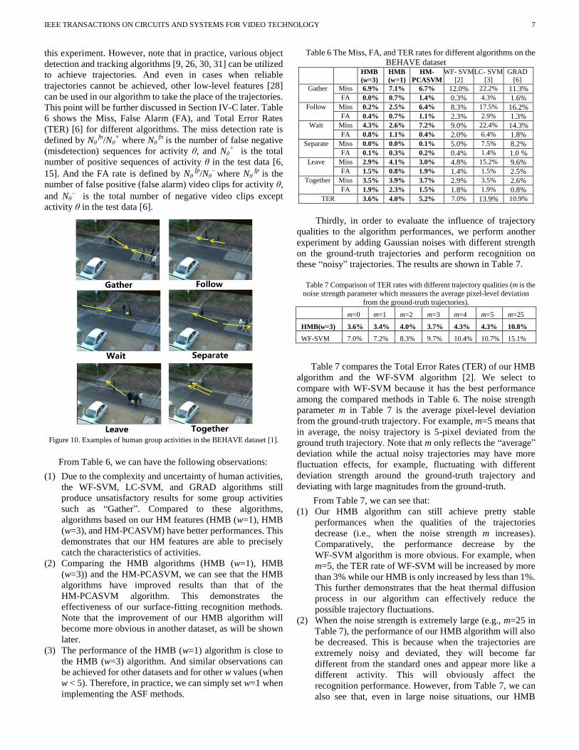
IEEE TRANSACTIONS ON CIRCUITS AND SYSTEMS FOR VIDEO TECHNOLOGY 7

this experiment. However, note that in practice, various object

detection and tracking algorithms [9, 26, 30, 31] can be utilized

to achieve trajectories. And even in cases when reliable

trajectories cannot be achieved, other low-level features [28]

can be used in our algorithm to take the place of the trajectories.

This point will be further discussed in Section IV-C later. Table

6 shows the Miss, False Alarm (FA), and Total Error Rates

(TER) [6] for different algorithms. The miss detection rate is

defined by Nθ fn

/Nθ+ where Nθ

fn is the number of false negative

(misdetection) sequences for activity θ, and Nθ+ is the total

number of positive sequences of activity θ in the test data [6,

15]. And the FA rate is defined by Nθ fp

/Nθ

where Nθ fp

is the

number of false positive (false alarm) video clips for activity θ,

and Nθ is the total number of negative video clips except

activity θ in the test data [6].

Figure 10. Examples of human group activities in the BEHAVE dataset [1].

From Table 6, we can have the following observations:

(1) Due to the complexity and uncertainty of human activities,

the WF-SVM, LC-SVM, and GRAD algorithms still

produce unsatisfactory results for some group activities

such as “Gather”. Compared to these algorithms,

algorithms based on our HM features (HMB (w=1), HMB

(w=3), and HM-PCASVM) have better performances. This

demonstrates that our HM features are able to precisely

catch the characteristics of activities.

(2) Comparing the HMB algorithms (HMB (w=1), HMB

(w=3)) and the HM-PCASVM, we can see that the HMB

algorithms have improved results than that of the

HM-PCASVM algorithm. This demonstrates the

effectiveness of our surface-fitting recognition methods.

Note that the improvement of our HMB algorithm will

become more obvious in another dataset, as will be shown

later.

(3) The performance of the HMB (w=1) algorithm is close to

the HMB (w=3) algorithm. And similar observations can

be achieved for other datasets and for other w values (when

w < 5). Therefore, in practice, we can simply set w=1 when

implementing the ASF methods.

Table 6 The Miss, FA, and TER rates for different algorithms on the

BEHAVE dataset HMB

(w=3)

HMB

(w=1)

HM-

PCASVM

WF- SVM [2]

LC- SVM [3]

GRAD [6]

Gather Miss 6.9% 7.1% 6.7% 12.0% 22.2% 11.3%

FA 0.0% 0.7% 1.4% 0.3% 4.3% 1.6%

Follow Miss 0.2% 2.5% 6.4% 8.3% 17.5% 16.2%

FA 0.4% 0.7% 1.1% 2.3% 2.9% 1.3%

Wait Miss 4.3% 2.6% 7.2% 9.0% 22.4% 14.3%

FA 0.8% 1.1% 0.4% 2.0% 6.4% 1.8%

Separate Miss 0.0% 0.0% 0.1% 5.0% 7.5% 8.2%

FA 0.1% 0.3% 0.2% 0.4% 1.4% 1.0 %

Leave Miss 2.9% 4.1% 3.0% 4.8% 15.2% 9.6%

FA 1.5% 0.8% 1.9% 1.4% 1.5% 2.5%

Together Miss 3.5% 3.9% 3.7% 2.9% 3.5% 2.6%

FA 1.9% 2.3% 1.5% 1.8% 1.9% 0.8%

TER 3.6% 4.0% 5.2% 7.0% 13.9% 10.9%

Thirdly, in order to evaluate the influence of trajectory

qualities to the algorithm performances, we perform another

experiment by adding Gaussian noises with different strength

on the ground-truth trajectories and perform recognition on

these “noisy” trajectories. The results are shown in Table 7.

Table 7 Comparison of TER rates with different trajectory qualities (m is the

noise strength parameter which measures the average pixel-level deviation

from the ground-truth trajectories).

m=0 m=1 m=2 m=3 m=4 m=5 m=25

HMB(w=3) 3.6% 3.4% 4.0% 3.7% 4.3% 4.3% 10.8%

WF-SVM 7.0% 7.2% 8.3% 9.7% 10.4% 10.7% 15.1%

Table 7 compares the Total Error Rates (TER) of our HMB

algorithm and the WF-SVM algorithm [2]. We select to

compare with WF-SVM because it has the best performance

among the compared methods in Table 6. The noise strength

parameter m in Table 7 is the average pixel-level deviation

from the ground-truth trajectory. For example, m=5 means that

in average, the noisy trajectory is 5-pixel deviated from the

ground truth trajectory. Note that m only reflects the “average”

deviation while the actual noisy trajectories may have more

fluctuation effects, for example, fluctuating with different

deviation strength around the ground-truth trajectory and

deviating with large magnitudes from the ground-truth.

From Table 7, we can see that:

(1) Our HMB algorithm can still achieve pretty stable

performances when the qualities of the trajectories

decrease (i.e., when the noise strength m increases).

Comparatively, the performance decrease by the

WF-SVM algorithm is more obvious. For example, when

m=5, the TER rate of WF-SVM will be increased by more

than 3% while our HMB is only increased by less than 1%.

This further demonstrates that the heat thermal diffusion

process in our algorithm can effectively reduce the

possible trajectory fluctuations.

(2) When the noise strength is extremely large (e.g., m=25 in

Table 7), the performance of our HMB algorithm will also

be decreased. This is because when the trajectories are

extremely noisy and deviated, they will become far

different from the standard ones and appear more like a

different activity. This will obviously affect the

recognition performance. However, from Table 7, we can

also see that, even in large noise situations, our HMB

IEEE TRANSACTIONS ON CIRCUITS AND SYSTEMS FOR VIDEO TECHNOLOGY 8

algorithm can still achieve better performance than the

WF-SVM method.

(3) More importantly, note that our HMB algorithm is not

limited to trajectories. Instead, various low-level motion

features such as the optical flow [28] can also be included

into our algorithm to create heat maps for recognition.

Therefore, in cases when reliable trajectories cannot be

achieved (such as the m=25 case in Table 7), our algorithm

can also be extended by skipping the tracking step and

directly utilizing other low-level motion features for

performing group activity recognition. This point will be

further discussed in Section IV-C later.

(a) (b)

(c)

Figure 11. (a) The trajectories for the two complex activities; (b) The major

feature values for the WF-SVM algorithm [2]; (c) The HMs for the two

complex activities.

Table 8 Miss and TER rates for the complex activities HMB (w=1) MF-SVM

Exchange Miss 5.9% 50.0%

Return Miss 11.6% 43.8%

TER 8.8% 46.9%

Figure 12. The example frames of the “Exchange” and “Return” sequences and the qualitative results of on-line sub-activity recognition by using a

30-frame-long sliding window. The bars represent labels of each frame, red represents Approach, green represents Stay, and blue represents Separate.

Fourthly, in order to further demonstrate our HM features,

we perform another experiment for recognizing two complex

activities: “Exchange” (i.e. two people first approach each

other, stay together for a while and then separate) and “Return”

(i.e., two people first separate and then approach to each other

later). In this experiment, we extract 32 pair-trajectories from

the BEHAVE dataset for the two complex activities and

perform 75% training-25% testing. Some example frames are

shown in Figure 12. In Figure 11, (a) shows the trajectories of

the two complex activities, (b) shows the values of the major

features in the WF-SVM algorithm [2], and (c) shows the HM

surfaces. From Figure 11 (b), we can see that the features in the

WF-SVM algorithm cannot show much difference between the

two complex activities. Compared to (b), our HMs in (c) are

obviously more distinguishable. The recognition results for the

WF-SVM algorithm and our HMB algorithm are shown in

Table 8. The results in Table 8 further demonstrate the

effectiveness of our HM features in representing complex

group activities.

Finally, we evaluate our algorithm in recognizing the

sub-activities. Note that our algorithm can be easily extended to

recognize the sub-activities by using shorter sliding windows to

achieve the short-term trajectories instead of the entire

trajectories. By this way, we can also achieve on-the-fly

activity recognition at each time instant [6, 29]. In order to

demonstrate this point, Figure 12 shows the results by applying

a 30-frame-long sliding window to automatically recognize the

sub-activities inside the complex “Exchange” and “Return”

video sequences. From Figure 12, we can see that our HMB

algorithm can also achieve satisfying recognition results for the

sub-activities inside the long-term sequences. Besides, our

algorithm is also able to recognize both the long-term activities

and the short-term activities by simultaneously introducing

multiple sliding windows with different lengths. By this way,

both the sub-activities of the current clip and the complex

activities of the long-term clip can be automatically recognized.

B. Experimental results for the traffic dataset

In this sub-section, we perform two experiments on the

traffic datasets.

Firstly, we perform an experiment on a traffic dataset for

recognizing group activities among vehicles in the crossroad.

The dataset is constructed from 20 long surveillance videos

taken by different cameras. Seven vehicle group activities are

defined as in Table 9 and some example activities are shown in

Figure 13. We select 245 video clips from the dataset where

each activity includes 35 video clips and each clip includes two

trajectories. In this dataset, the trajectories are achieved by first

using our proposed object detection method [26] to detect the

vehicles and then using the particle-filtering-based tracking

method [9, 31] to track the detected vehicles. The Miss, FA,

and TER of different algorithms are shown in Table 10.

Table 9 Definitions of the vehicle group activities Turn A car goes straight and a car in another lane turns right.

Follow A car is followed by a car in the same lane.

Side Two cars go side-by-side in two lanes.

Pass A car passes the crossroad and a car in the other direction waits for

green light.

Overtake A car is overtaken by a car in a different lane.

Confront Two cars in opposite directions go by each other.

Bothturn Two cars in opposite directions turn right in the same time.

IEEE TRANSACTIONS ON CIRCUITS AND SYSTEMS FOR VIDEO TECHNOLOGY 9

From Table 9, we can see that the LC-SVM algorithm

produces less satisfactory results. This is because the group

activities in this dataset contain more complicated activities

that are not easily distinguishable by the causality and feedback

features [3]. Also, the performance of the WF-SVM and the

GRAD algorithms are still unsatisfactory in several activities

such as “Follow”, “Overtake”, and “Pass”. Compared to these,

the performances of our HM algorithms (HMB (w=1) and

HM-PCASVM) are obviously improved. Besides, the

performance of the HMB (w=1) is also improved from the

HM-PCASVM algorithm. These further demonstrate the

effectiveness of our proposed HM feature as well as our SF

recognition method.

Figure 13. Examples of the defined vehicle group activities.

Table 10 Miss, FA, and TER for different algorithms on the vehicle

group activity dataset HMB

(w=1)

HM-

PCASVM

WF-

SVM [2]

LC-

SVM [3]

GRAD

[6]

Turn Miss 2.9% 4.7% 2.0% 16.9% 10.7%

FA 0.5% 1.4% 0.5% 5.4% 4.1%

Follow Miss 11.4% 9.6% 22.9% 38.1% 15.4%

FA 0.5% 1.0% 4.4% 15.1% 5.9%

Side Miss 1.9% 0.1% 0.2% 16.5% 7.1%

FA 1.0% 1.9% 0.3% 1.0% 0.3%

Pass Miss 0.0% 5.7% 11.7% 17.6% 15.5%

FA 0.1% 0.0% 2.4% 1.5% 3.1%

Overtake Miss 5.7% 11.4% 47.1% 61.7% 36.6%

FA 0.5% 0.2% 4.9% 11.7% 3.8%

Confront Miss 5.6% 9.5% 3.9% 19.6% 12.4%

FA 1.9% 2.9% 1.5% 10.7% 8.3%

Bothturn Miss 2.9% 3.0% 1.2% 2.9% 4.2%

FA 1.0% 1.4% 0.5% 1.0% 2.9%

TER 4.5% 7.8% 12.1% 21.5% 14.6%

Furthermore, it should be noted that there are two important

challenging characteristics for the traffic dataset: (1) The

videos in the dataset are taken from different cameras (as in

Figure 13). This makes the trajectories vary a lot for the same

activity. (2) Within each video, there are also large scale

variations (i.e., the object size is much larger at the front region

than that in the far region, as shown in Figure 13). Because of

this, same activities from different regions may also have large

variations and are difficult to be differentiated. These

challenging characteristics partially lead to the low

performance in the compared algorithms (WF-SVM, LC-SVM,

and GRAD). However, comparatively, these variations in scale

and camera view are much less obvious in our HM algorithms

(HMB (w=1) and HM-PCASVM) by utilizing the proposed

KPB alignment method for eliminating the scale differences

and utilizing the proposed HM for effectively catching the

common characteristics of activities.

Secondly, we also perform another experiment with

different camera settings. In this experiment, we use the traffic

dataset in Figure 13 to train the HMs and then directly use these

HMs to recognize the activities from a new dataset as in Figure

14. The new dataset in Figure 14 includes 65 video clips taken

from a camera whose height, angle, and zoom are largely

different from the ones in Figure 13. The results are shown in

Table 11.

Figure 14. Examples of vehicle group activities in the new dataset.

From Table 11, we can see that when using the trained

models to recognize the activities in a dataset with different

camera settings, the performances of the compared algorithms

(WF-SVM, LC-SVM, and GRAD) are obviously decreased.

Comparatively, our HM algorithms (HMB (w=1) and

HM-PCASVM) can still produce reliable results. This

demonstrates that: (1) Our proposed key-point-based (KPB)

heat-map alignment method can effectively handle the heat

map differences due to different camera settings. (2) Our HMB

algorithm has the flexibility of directly applying the HMs

trained from one camera setting to the other camera settings.

IEEE TRANSACTIONS ON CIRCUITS AND SYSTEMS FOR VIDEO TECHNOLOGY 10

Table 11 Miss, FA, and TER for different algorithms by using the

HMs trained from the traffic dataset in Figure 13 to recognize the new

dataset in Figure 14 HMB

(w=1)

HM-

PCASVM

WF-

SVM[2]

LC-

SVM[5]

GRAD

[6]

Turn Miss 0.0% 0.0% 0.0% 38.5% 15.2%

FA 2.1% 3.6% 0.0% 13.5% 4.8%

Follow Miss 8.3% 7.7% 32.1% 46.2% 20.1%

FA 1.9% 0.0% 17.3% 13.5% 10.6%

Side Miss 12.8% 18.2% 28.6% 30.8% 35.5%

FA 4.1% 1.7% 0.0% 0.0% 0.0%

Pass Miss 0.0% 0.0% 0.0% 0.0% 0.0%

FA 0.0% 0.0% 9.2% 1.3% 3.1%

Overtake Miss 9.7% 15.1% 53.8% 61.5% 46.9%

FA 3.8% 7.2% 1.9% 7.7% 2.7%

Confront Miss 6.2% 8.7% 23.1% 46.2% 16.2%

FA 1.0% 0.0% 0.0% 3.8% 1.3%

Bothturn Miss 0.0% 0.0% 0.0% 0.0% 0.0%

FA 0.0% 1.5% 3.1% 9.2% 3.3%

TER 6.9% 10.1% 27.7% 44.6% 32.9%

C. Experimental results for the UMN dataset

Finally, in order to demonstrate that our algorithm can also

be extended to other low-level motion features [28], we

perform another experiment by using the optical flows for

recognition.

Figure 15. The qualitative results of using our HMB algorithm for abnormal

detection in the UMN dataset. The bars represent the labels of each frame, green represents normal and red represents abnormal.

The experiment is performed on the UMN dataset [22] which

contains videos of 11 different scenarios of an abnormal escape

event in 3 different scenes including both indoor and outdoor.

Each video starts with normal behaviors and ends with the

abnormal behavior (i.e., escape). In this experiment, we first

compute the optical flow between the current and the previous

frames. Then patches with high optical-flow magnitudes will be

viewed as the heat sources for creating the heat maps (HMs)

and these heat maps will be utilized for activity recognition in

our HMB algorithm. A sliding window of 30 frames is used as

the basic video clip and one HM is generated from each clip. By

this way, we can achieve 257 video clips. We randomly select 5

normal behavior HMs and 5 abnormal behavior HMs as the

training set to classify the rest 247 video clips. Furthermore, we

set w in Eqn. (5) as 1.

Figure 15 shows some example frames of the UMN dataset

and compares the normal/abnormal classification results of our

algorithm with the ground truth. Furthermore, Figure 16

compares the ROC curves between our algorithm (HMB+

Optical Flow) and three other algorithms: the optical flow only

method (Optical Flow) [20, 28], the Social Force Model (SFM)

[20], and the Velocity-Field Based method (VFB) [21].

From Figure 15 and 16, we can have the following

observations:

(1) From Figure 15, we can see that the UMN dataset includes high density of people where reliable tracking is difficult.

However, our HMB algorithms can still achieve satisfying

normal/abnormal classification results by using the optical

flow features. This demonstrates the point that when

reliable trajectories cannot be achieved, our algorithm can

be extended by skipping the tracking step and directly

utilizing the low-level motion features to perform group

activity recognition.

(2) From Figure 15, we can see that our algorithm can perform

online normal/abnormal activity recognition for each time

instant by using a 30-frame-long sliding window. This

further demonstrates that our algorithm is extendable to

on-the-fly and sub-activity recognitions.

(3) Our HMB algorithm can achieve similar or better results

than the existing social-force-based methods [20-21] when

detecting the UMN dataset. This demonstrates the

effectiveness of our HMB algorithm. Although other

social-force-based methods [23] may have further

improved results on the UMN dataset, the performance of

our HMB algorithm can also be further improved by: (a)

using more reliable motion features (such as the

trajectories of the local spatio-temporal interest points [23])

to take the place of the optical flow, (b) including more

training samples (note that in this experiment, only five

normal clips and five abnormal clips are used for training

in our algorithm).

(4) More importantly, compared with the social-force-based

methods [20, 21, 23], our HMB algorithm also has the

following advantages:

(a) Most social-force-based methods [20, 21, 23] are

more focused on the relative movements among the

objects (e.g., whether two objects are approaching or

splitting) while the objects’ absolute movements in

the scene are neglected (e.g., whether an object is

stand still or moving in the scene). Thus, these

methods will have limitations in differentiating

activities with similar relative movements but

different absolute movements (such as “Wait” and

“Gather” in Figure 10 or “Confront” and “Bothturn”

in Figure 13). Comparatively, the heat map features

in our HMB algorithm can effectively embed both the

relative and absolute movements of the objects.

IEEE TRANSACTIONS ON CIRCUITS AND SYSTEMS FOR VIDEO TECHNOLOGY 11

(b) Since the interaction forces used in the

social-force-based methods [20, 21, 23] cannot

effectively reflect the correlation changes over time

(e.g., two objects first approach and then split), they

also have limitations in differentiating activities with

complex correlation changes such as “Return” and

“Exchange”. Comparatively, since our HM features

include rich information about the temporal

correlation variations among objects, these complex

activities can be effectively handled by our algorithm.

(c) Since our HM features can effectively distinguish the

motion patterns between the normal and abnormal

behaviors, our algorithm can achieve good

classification results with only a small number of

training samples (in this experiment, only five

30-frame-long normal clips and five 30-frame

abnormal clips are needed for training in our

algorithm). Comparatively, more training samples are

required to construct reliable models for the

social-force-based methods [20, 21, 23].

Figure 16. ROC curves of different methods in abnormal detection in the UMN

dataset.

IV. CONCLUSION

In this paper, we propose a new heat-map-based (HMB)

algorithm for group activity recognition. We propose to create

the heat map (HM) for representing the group activities.

Furthermore, we also propose to use a key-point-based method

for aligning different HMs and a surface-fitting method for

recognizing activities. Experimental results demonstrate the

effectiveness of our algorithm.

REFERENCES

[1] BEHAVE dataset: http://homepages.inf.ed.ac.uk/rbf/BEHAVE.

[2] Y. Zhou, S. Yan, and T. Huang, “Pair-Activity Classification by Bi-Trajectory Analysis,” IEEE Conf. Computer Vision and Pattern

Recogntion (CVPR), pp. 1-8, 2008.

[3] B. Ni, S. Yan, and A. Kassim, “Recognizing Human Group Activity with Localized Causalities,” IEEE Conf. Computer Vision and Pattern

Recogntion (CVPR), pp. 1470-1477, 2009. [4] Z. Cheng, L. Qin, Q. Huang, S. Jiang, and Q. Tian, “Group Activity

Recognition by Gaussian Process Estimation,” Int’l Conf. Pattern

Recognition (ICPR), pp. 3228-3231, 2010. [5] Y. Chen, W. Lin, H. Li, H. Luo, Y. Tao, and D. Liu, “A New

Package-Group-Transmission-based Algorithm for Human Activity Recognition in Videos,” IEEE Visual Communications and Image

Processing(VCIP), pp. 1-4, 2011.

[6] W. Lin, M.-T. Sun, R. Poovendran, and Z. Zhang, “Group event detection

with a varying number of group members for video surveillance,” IEEE

Trans. Circuits Syst. Video Technol., vol. 20, no. 8, pp. 1057-1067, 2010. [7] C. Goodall. “Procrustes Methods in the Statistical Analysis of Shape,”

Journal of the Royal Statistical Society, vol. 53, no. 3, pp. 285-339, 1991. [8] Y. Fang, M. Sun, M. Kim, and K. Ramani, “Heat-Mapping: A Robust

Approach toward Perceptually Consistent Mesh Segmentation,” IEEE

Conf. Computer Vision and Pattern Recognition (CVPR), pp. 2145-2152, 2011.

[9] D. Comaniciu, V. Ramesh, and P. Meer, “Kernel-based Object Tracking,” IEEE Trans. Pattern Analysis and Machine Intelligence, vol. 25, no. 5, pp.

564–574, 2003.

[10] H. Carslaw and J. Jaeger, Conduction of Heat in Solids, Oxford University Press, 1986.

[11] A. Girgensohn, F. Shipman, and L. Wilcox, “Determining Activity Patterns in Retail Spaces through Video Analysis,” ACM Multimedia, pp.

889-892, 2008.

[12] W. A. Hoff and J. W. Howard, “Activity Recognition in a Dense Sensor Network,” Int’l Conf. Sensor Networks and Applications (SNA), 2009.

[13] T. F. Cootes and C. J. Taylor, “Statistical Models of Appearance for Computer Vision,” Image Science and Biomedical Engineering, Univ.

Manchester, Manchester, U.K.,Tech. Rep., 2004.

[14] T. Hastie, R. Tibshirani, and J. H. Friedman, “The Elements of Statistical

Learning,” Springer, 2003.

[15] W. Lin, M.-T. Sun, R. Poovendran, and Z. Zhang, “Activity Recognition using a Combination of Category Components and Local Models for

Video Surveillance,” IEEE Trans. Circuits Syst. Video Technol., vol. 18,

no. 8, pp. 1128-1139, 2008. [16] C. Chang and C. Lin, “LIBSVM: A Library for Support Vector

Machines,” ACM Trans. Intelligent Syst. Tech., vol. 2, pp. 1-27, 2011. [17] C. Wang, J. Zhang, J. Pu, X. Yuan, and L. Wang, "Chrono-Gait Image: A

Novel Temporal Template for Gait Recognition," European Conference

on Computer Vision (ECCV), pp. 257-270, 2010. [18] L. Bao and S. Intille, “Activity Recognition from User-Annotated

Acceleration Data,” Int’l Conf. Pervasive Computing (PERVASIVE), vol. 3001, pp. 1-17, 2004.

[19] C. Rao, M. Shah, and T. Syeda-Mahmood, “Action Recognition based on

View Invariant Spatio-Temporal Analysis,” ACM Multimedia, pp. 518-527, 2003.

[20] R. Mehran, A. Oyama, and M. Shah, “Abnormal Crowd Behavior

Detection using Social Force Model,” IEEE Conf. Computer Vision and Pattern Recogntion (CVPR), pp. 935-942, 2009.

[21] J. Zhao, Y. Xu, X. Yang, and Q. Yan, “Crowd Instability Analysis Using Velocity-Field Based Social Force Model,” Visual Communications and

Image Processing (VCIP), pp. 1-4, 2011.

[22] Unusual Crowd Activity Dataset: http://mha.cs.umn.edu/Movies/Crowd- Activity-All.avi

[23] X. Cui, Q. Liu, M. Gao, and D. N. Metaxas, “Abnormal Detection Using Interaction Energy Potentials,” IEEE Conf. Computer Vision and Pattern

Recogntion (CVPR), pp. 3161-3167, 2011.

[24] B. Zhan, D. N. Monekosso, P. Remagnino, S. A. Velastin, and L. Xu, “Crowd Analysis: A Survey,” Machine Vision and Application, vol. 19, pp.

345-357, 2008. [25] J. C. S. Jacques Junior, S. R. Musse, and C. R. Jung, “Crowd Analysis

Using Computer Vision Techniques,” Signal Processing Magazine, vol.

27, pp. 66-77, 2010. [26] X. Su, W. Lin, X. Zhen, X. Han, H. Chu, and X. Zhang, “A New

Local-Main-Gradient-Orientation HOG and Contour Differences based Algorithm for Object Classification,” IEEE Int’l Symposium on Circuits

and Systems (ISCAS), 2013.

[27] H. Chu, W. Lin, J. Wu, X. Zhou, Y. Chen, and H. Li, "A New Heat-Map-based Algorithm for Human Group Activity Recognition",

ACM Multimedia, 2012. [28] B. D. Lucas and T. Kanade, “An iterative image registration technique

with an application to stereo vision,” Proceedings of Imaging

Understanding Workshop, 1981. [29] S. Chiappino, P. Morerio, L. Marcenaro, E. Fuiano, G. Repetto, C.S.

Regazzoni, "A multi-sensor cognitive approach for active security monitoring of abnormal overcrowding situations," Int’l Conf. Information

Fusion (FUSION) , pp.2215-2222, 2012.

[30] G. Wu, Y. Xu, X. Yang, Q. Yan, K. Gu, “Robust object tracking with bidirectional corner matching and trajectory smoothness algorithm,” Int’l

Workshop on Multimedia Signal Processing, pp. 294-298, 2012. [31] R. Hess and A. Fern, “Discriminatively Trained Particle Filters for

Complex Multi-Object Tracking,” IEEE Conf. Computer Vision and

Pattern Recognition (CVPR), pp. 240-247, 2009.

IEEE TRANSACTIONS ON CIRCUITS AND SYSTEMS FOR VIDEO TECHNOLOGY 12

Hang Chu is currently an undergraduate student in the Department of Electronic Engineering,

School of Electronic Information and Electrical Engineering, Shanghai Jiao Tong University,

Shanghai, China. He will receive his B.S. degree

in July 2013. His current research interest is statistical learning and its applications in

computer vision.

Weiyao Lin received the B.E. degree from

Shanghai Jiao Tong University, China, in 2003, the M.E. degree from Shanghai Jiao Tong

University, China, in 2005, and the Ph.D degree

from the University of Washington, Seattle, USA, in 2010, all in electrical engineering.

Currently, he is an associate professor at the Department of Electronic Engineering, Shanghai

Jiao Tong University.

His research interests include video processing, machine learning, computer vision

and video coding & compression.

Jianxin Wu received his BS & MS degree in

computer science from Nanjing University, and

the PhD degree in computer science from Georgia Institute of Technology. He is currently a

professor in Nanjing University, and was an assistant professor in Nanyang Technological

University. His research interests are computer

vision and machine learning.

Bin Sheng received his BA degree in English and

BE degree in Computer Science from Huazhong University of Science and Technology in 2004,

MS degree in software engineering from the University of Macau in 2007, and PhD degree in

Computer Science from The Chinese University

of Hong Kong in 2011. He is currently an assistant professor in the Department of

Computer Science and Engineering at Shanghai Jiao Tong University. His research interests

include virtual reality, computer graphics, and

image based techniques.

Zhenzhong Chen received the B.Eng. degree

from the Huazhong University of Science and

Technology, Wuhan, China, and the Ph.D. degree from the Chinese University of Hong Kong

(CUHK), Shatin, Hong Kong, both in electrical engineering.

He is currently Member of Technical Staff at

MediaTek USA Inc. He was a Lee Kuan Yew Research Fellow and a Principal Investigator

with the School of Electrical and Electronic Engineering, Nanyang Technological University

(NTU), Singapore, and the European Research Consortium for Informatics and

Mathematics Fellow (ERCIM Fellow) with the National Institute for Research in Computer Science and Control (INRIA), France. He held visiting positions

with Polytech’Nantes, Nantes, France, Universit e Catholique de Louvain, Louvain-la-Neuve, Belgium, and Microsoft Research Asia, Beijing, China. His

current research interests include visual perception, visual signal processing,

and multimedia communications. He is a voting member of the IEEE Multimedia Communications

Technical Committee (MMTC) and an invited member of the IEEE MMTC Interest Group of Quality of Experience for Multimedia Communications from

2010 to 2012. He has served as a guest editor of special issues for IEEE MMTC

E-Letter and the Journal of Visual Communication and Image Representation. He has served as the Co-Chair of International Workshop on Emerging

Multimedia Systems and Applications 2012 (EMSA 2012). He has co-organized several special sessions at international conferences, including

IEEE ICIP 2010, ICME 2010, and Packet Video 2010, and has served as a

technical program committee member of IEEE ICC, GLOBECOM, CCNC, ICME, and so on. He received the CUHK Faculty Outstanding Ph.D. Thesis

Award, the Microsoft Fellowship, and the ERCIM Alain Bensoussan Fellowship. He is a member of SPIE.