Embed Size (px)
Citation preview

IEEE TRANS. ON IMAGE PROCESSING, VOL. X, NO. XX, XXXX 1
Variational Bayesian Blind Deconvolution
Using A Total Variation PriorS. Derin Babacan, Student Member, IEEE, Rafael Molina, Member, IEEE,
Aggelos K. Katsaggelos, Fellow, IEEE
Abstract
In this paper we present novel algorithms for total variation (TV) based blind deconvolution and
parameter estimation utilizing a variational framework. Using a hierarchical Bayesian model, the unknown
image, blur, and hyperparameters for the image, blur, and noise priors are estimated simultaneously. A
variational inference approach is utilized so that approximations of the posterior distributions of the
unknowns are obtained, thus providing a measure of the uncertainty of the estimates. Experimental
results demonstrate that the proposed approaches provide higher restoration performance than non-TV
based methods without any assumptions about the unknown hyperparameters.
Index Terms
Blind deconvolution, total variation, variational methods, parameter estimation, Bayesian methods.
I. INTRODUCTION
Image acquisition systems introduce blurring degradation to the acquired image. In many applications
it is desired to undo this process. Blind deconvolution refers to a class of problems when the original
S. Derin Babacan is with the Department of Electrical Engineering and Computer Science, Northwestern University, IL, USA.
e-mail: [email protected]
Rafael Molina is with the Departamento de Ciencias de la Computacion e I.A. Universidad de Granada, Spain. e-mail:
Aggelos K. Katsaggelos is with the Department of Electrical Engineering and Computer Science, Northwestern University,
IL, USA. e-mail: [email protected]
Preliminary results of this work can be found in [1].
This work was supported in part by the “Comision Nacional de Ciencia y Tecnologa” under contract TIC2007-65533 and the
Spanish research programme Consolider Ingenio 2010: MIPRCV (CSD2007-00018).

IEEE TRANS. ON IMAGE PROCESSING, VOL. X, NO. XX, XXXX 2
image is estimated from the degraded observations where the exact information about the degradation and
noise is not available. The blind deconvolution problem is very challenging since it is hard to infer the
original image and the unknown degradation only from the observed image. Moreover, the degradation
is generally nonlinear (due to saturation, quantization, etc.) and spatially varying (lens imperfections,
nonuniform motion, etc). However, most of the work in the literature approximates the degradation
process by a linear spatially invariant (LSI) system, where the original image is convolved by the blur
point spread function (PSF) and independent white Gaussian noise is added to the blurred image.
There are many applications where the PSF is unknown or partially known, where blind deconvolution is
needed, such as astronomical imaging, remote sensing, microscopy, medical imaging, optics, photography,
super-resolution applications, and motion tracking applications, among others.
A number of methods have been proposed to address the blind deconvolution problem. Reviews of the
major approaches can be found in [2] and [3]. Blind deconvolution methods can be classified into two
main categories based on the stage where the blur is identified. In the a priori blur identification methods,
the PSF is estimated separately from the original image, and then used in an image restoration method
[4]. The second category of methods, referred to as joint identification methods, provide an estimate of
the original image and blur simultaneously [5]–[11]. Typically these methods incorporate prior knowledge
about the original image, degradation, and noise in the estimation process. This prior knowledge can be
exploited with the use of convex sets and regularization techniques, or with the use of the Bayesian
framework with prior models on the unknown parameters.
Methods based on the Bayesian formulation are of the most commonly used methods in blind de-
convolution. Such methods introduce prior models on the image, blur, and their model parameters,
which impose constraints on the estimates and act as regularizers. Simultaneous autoregressive (SAR),
conditional autoregressive (CAR), and Gaussian models are some of the commonly used priors for the
image and blur. With the use of these mathematical models one can try to model different types of blurs,
like out-of-focus, motion, or Gaussian blurs, and different characteristics of the original image, such as
smoothness and sharp edges.
Recently there has been an interest in applying variational methods to the blind deconvolution problem.
These methods aim at obtaining approximations to the posterior distributions of the unknowns with the
use of the Kullback-Leibler divergence [12]. This variational methodology to the blind deconvolution
problem in a Bayesian formulation has been utilized in [6] [7] [13] [14] .
In this paper we propose to use variational methods for the blind deconvolution problem by incorpo-
rating a total variation (TV) function as the image prior, and a SAR model as the blur prior. Although the

IEEE TRANS. ON IMAGE PROCESSING, VOL. X, NO. XX, XXXX 3
TV model has been used in a regularization formulation in blind deconvolution before (see, for example,
[5]), to the best of our knowledge, no work has been reported on the simultaneous estimation of the
model parameters, image, and blur. Previous works attempted to solve for the unknown image and the
blur, but the model parameters are manually selected [5] [15]. Moreover, we cast the TV-based blind
deconvolution into a Bayesian estimation problem, which provides advantages in blind deconvolution,
such as means to estimate the uncertainties of the estimates. We develop two novel variational methods
based on the hierarchical Bayesian formulation, and provide approximations to the posterior distributions
of the image, blur, and model parameters rather than point estimates.
This paper is organized as follows. In Section II we present the hierarchical Bayesian model and the
prior models on the observation, the image and the blur. Section III describes the variational approximation
method utilized in the Bayesian inference. We present experimental results in Section IV and conclusions
are drawn in Section V.
II. HIERARCHICAL BAYESIAN MODELING
The image degradation model is often presented as a discrete linear and spatially invariant system,
which can be expressed in matrix-vector form as
y = Hx + n, (1)
where the vectors x, y, and n represent respectively the original image, the available noisy and blurred
image, and the noise with independent elements of variance σ2n = β−1, and H represents the unknown
block-circulant blurring matrix formed by the degradation system with impulse response h. The images
are of size N = n × m, so that the vectors y and x are of size N × 1 and the matrix H is of size
N ×N . Note that Eq. (1) can also be written as y = Xh + n by forming the matrix X similarly to H.
The blind deconvolution problem calls for finding estimates of x and h given y, and using knowledge
about n and possibly x and h.
In Bayesian models, all unknown parameters are treated as stochastic quantities and probability dis-
tributions are assigned to them. The unknown parameters x and h are assigned prior distributions
p(x|αim) and p(h|αbl), which model the knowledge about the nature of the original image and the blur,
respectively. The observation y is also a random process with the corresponding conditional distribution
p(y|x,h, β). Clearly, these distributions depend on the model parameters αim, αbl, and β, which are called
hyperparameters. The meaning of the hyperparameters will become clear when the prior distributions
are defined below. In this paper, we will denote the set of hyperparameters as Ω = (αim, αbl, β).

IEEE TRANS. ON IMAGE PROCESSING, VOL. X, NO. XX, XXXX 4
The Bayesian modeling of this problem firstly requires the definition of the joint probability distribution
of all unknown and observed quantities, which is factorized as
p(αim, αbl, β,x,h,y) = p(αim, αbl, β)p(x|αim)p(h|αbl)p(y|x,h, β). (2)
To alleviate the ill-posed nature of the blind deconvolution problem, prior knowledge about the unknown
image and the blur is incorporated through the use of the prior distributions. If the hyperparameters are not
assumed known, they have to be estimated simultaneously with the unknown parameters. To achieve this
we utilize a hierarchical model which has two steps: In the first step, the a priori probability distributions
p(h|αbl) and p(x|αim) and the ‘conditional distribution p(y|x,h, β) are formed that model the structure
of the PSF, the original image, and the noise, respectively. In the second stage, hyperpriors on the
hyperparameters β, αim and αbl are defined to model the prior knowledge of their values.
In the next subsections we first describe the prior models for the image and the PSF as well as the
observation model we use in the first stage of the hierarchical Bayesian paradigm. We then proceed to
explain the hyperprior distributions on the hyperparameters.
A. First stage: Prior models on the observation, PSF and image
We assume that the degradation noise is independent and Gaussian with zero mean and variance equal
to β−1, and consequently we have
p(y|x, h, β) ∝ βN/2 exp[−β
2‖ y −Hx ‖2
]. (3)
For the image prior we adopt the TV function, that is,
p(x|αim) ∝ 1ZTV(αim)
exp [−αimTV(x)] , (4)
where ZTV(αim) is the partition function. The TV function is defined as
TV(x) =∑i
√(∆h
i (x))2 + (∆vi (x))2, (5)
where the operators ∆hi (x) and ∆v
i (x) correspond to, respectively, the horizontal and vertical first order
differences at pixel i. In other words, ∆hi (x) = xi − xl(i) and ∆v
i (x) = xi − xa(i), with l(i) and a(i)
denoting the nearest horizontal and vertical neighbors of pixel i, respectively. The TV prior has become
very popular recently in the restoration literature because of its edge-preserving property by not over-
penalizing discontinuities in the image while imposing smoothness [16]. Note that the TV prior is an
improper prior (see, for example, [17]) but if integrated in an adequate affine subspace (a hyperplane)
the density is normalizable.

IEEE TRANS. ON IMAGE PROCESSING, VOL. X, NO. XX, XXXX 5
The calculation of the partition function ZTV(αim) =∫
exp [−αimTV(x)] dx in Eq. (4) presents a
major difficulty. We can, however, approximate it by using [18]∫ ∫exp
[−αim
√s2 + t2
]dsdt = 2π/α2
im. (6)
Therefore, the TV prior can be approximated as
p(x|αim) = c αN/2im exp [−αimTV(x)] , (7)
with c a constant.
We utilize the SAR model for the blur prior, that is,
p(h|αbl) ∝ αM/2bl exp
−1
2αbl ‖ Ch ‖2, (8)
where C denotes the discrete Laplacian operator, α−1bl is the variance of the Gaussian distribution, and
M is the support of the blur, which is assumed to be the same as the image support. Note that in Eq. (8),
M should in theory be replaced by M −1, because CTC is singular. The SAR model is very efficient in
estimating smooth PSFs, for instance, a Gaussian PSF modeling long-term atmospheric turbulence. Our
selection of the SAR prior is based on the fact that we aim at restoring images which have been blurred
with smoothly varying PSFs. As we will show in the experiments, for such PSFs the proposed prior
works better than TV based blur priors (e.g., [5] [15]). On the other hand, a TV blur prior models better
piecewise smooth priors such as the rectangular shaped and out of focus blurs. This is in agreement with
the fact that TV models are better image priors than autoregressive models.
B. Second stage: Hyperpriors on the hyperparameters
The hyperparameters are important in determining the performance of the algorithms to a great extent.
In most previous work, the hyperparameters are assumed known. However, this requires a significant
amount of supervision in the restoration process. To ameliorate this problem, in this work they are
assumed unknown and are simultaneously estimated by introducing a second stage in the Bayesian
model.
Finding the form of the hyperprior distributions that allows for easy calculation of the posterior distribu-
tion p(Ω,x,h|y) is a major problem in Bayesian literature. A desired property for the hyperprior is to be
conjugate [19], that is, to have the same functional form with the product p(x|αim)p(h|αbl)p(y|x,h, β),
so that the posterior distribution will have the same functional form as the prior distribution, only the
parameters will be updated by the sample information.

IEEE TRANS. ON IMAGE PROCESSING, VOL. X, NO. XX, XXXX 6
Fig. 1. Graphical model showing relationships between variables.
Based on the above, we utilize the Gamma distribution for the hyperparameters αim, αbl and β, since
it is the conjugate prior for the inverse variance (precision) of the Gaussian distribution. The Gamma
distribution is defined by
p(ω) = Γ(ω|aoω, boω) =(boω)−a
oω
Γ(aoω)ωa
oω−1 exp
[− ωboω
], (9)
where ω > 0 denotes a hyperparameter, boω > 0 is the scale parameter, and aoω > 0 is the shape parameter,
both of which are assumed to be known and introduce our prior knowledge on the hyperparameters. We
discuss the selection of the shape and scale parameters in the experimental section. The gamma distribution
has the following mean, variance and mode:
E[ω] = aoωboω, V ar[ω] = aoω(boω)2,Mode[ω] = (aoω − 1)boω. (10)
Note that in addition to the advantage of the already described conjugacy property, the Gamma distri-
bution allows for the incorporation of more vague or precise knowledge about the precision parameters.
By simply replacing aoω by aoω · λ and boω by boω/λ, another Gamma distribution with the same mean
but with variance aoωboω · λ can be obtained. Therefore, by varying λ we maintain the same mean of the
precision parameter ω but can vary the confidence on this mean.
Finally, by combining the first and second stage of the hierarchical Bayesian model, the joint distribution
in Eq. (2) can be defined. The dependencies in this joint probability model are shown in graphical form
in Fig. (1) using a directed acyclic graph.

IEEE TRANS. ON IMAGE PROCESSING, VOL. X, NO. XX, XXXX 7
III. BAYESIAN INFERENCE AND VARIATIONAL APPROXIMATION OF THE POSTERIOR DISTRIBUTIONS
We will denote the set of all unknowns by Θ = (Ω,x,h) = (αim, αbl, β,x,h). As is widely known,
Bayesian inference is based on the posterior distribution
p(Θ | y) = p(αim, αbl, β,x,h|y) =p(αim, αbl, β,x,h,y)
p(y), (11)
where p(αim, αbl, β,x,h,y) is given by Eq. (2). However, the posterior p(Θ | y) is intractable, since
p(y) =∫ ∫ ∫ ∫ ∫
p(α, β,x,h,y) dh dx dβ dαbl dαim (12)
can not be calculated analytically. Therefore, we consider an approximation of p(Θ | y) by a simpler
tractable distribution q(Θ) following the variational methodology [20]. The distribution q(Θ) will be
found by minimizing the Kullback-Leibler (KL) divergence, given by [12], [21]
CKL(q(Θ) ‖ p(Θ|y)) =∫
q(Θ) log(
q(Θ)p(Θ|y)
)dΘ =
∫q(Θ) log
(q(Θ)
p(Θ,y)
)dΘ + const, (13)
which is always nonnegative and equal to zero only when q(Θ) = p(Θ|y). In order to obtain a tractable
approximation, the family of distributions q(Θ) are restricted utilizing the mean field approximation [22]
so that q(Θ) = q(Ω)q(x)q(h), where q(Ω) = q(αim)q(αbl)q(β).
However, the use of the TV prior makes the integral in Eq. (13) difficult to evaluate even with this
factorization. Therefore, a majorization of the TV prior is utilized to find an upper bound of the KL
divergence. First we define the following functional M(αim,x,u), for αim, x, and any N−dimensional
vector u ∈ (R+)N
M(αim,x,u) = αN/2im exp
[−αim
2
∑i
(∆hi (x))2 + (∆v
i (x))2 + ui√ui
]. (14)
Now, using the following inequality for w ≥ 0 and z > 0
√wz ≤ w + z
2⇒√w ≤ w + z
2√z. (15)
we obtain from Eq. (7)
exp[−αimTV(x)] = exp
[−αim
∑i
√(∆h
i (x))2 + (∆vi (x))2
]
≥ exp
[−αim
2
∑i
(∆hi (x))2 + (∆v
i (x))2 + ui√ui
], (16)
which leads to the following lower bound for the image prior
p(x|αim) ≥ c · M(αim,x,u), (17)

IEEE TRANS. ON IMAGE PROCESSING, VOL. X, NO. XX, XXXX 8
and the following lower bound for the joint probability distribution
p(Θ,y) ≥ c · p(Ω) M(αim,x,u) p(h|αbl) p(y|x,h, β)
= F(Θ,u,y). (18)
For θ ∈ αim, αbl, β,x,h let us denote by Θθ the subset of Θ with θ removed; for instance, if θ = x,
Θx = (αim, αbl, β,h). Then, utilizing the lower bound F(Θ,u,y) for the joint probability distribution
in Eq. (13) we obtain an upper bound for the KL divergence as follows
M(q(Θ)) =∫
q(Θ) log(
q(Θ)p(Θ,y)
)dΘ
≤∫
q(θ)(∫
q(Θθ) log(
q(θ)q(Θθ)F(Θ,u,y)
)dΘθ
)dθ = M(q(Θ), u) (19)
Therefore, we minimize this upper bound instead of minimizing the KL divergence in Eq. (13). Note
that the form of the inequality in (19) suggests an alternating (cyclic) optimization strategy where the
algorithm cycles through the unknown distributions and replaces each with a revised estimate given
by the minimum of (19) with the other distributions held constant. Thus, given q(Θθ), the posterior
approximation q(θ) can be computed by solving
q(θ) = arg minq(θ)
CKL(q(Θθ)q(θ) ‖ F(Θ,u,y)). (20)
In order to solve this equation, we note that differentiating the integral on the right hand side in Eq. (19)
with respect to q(θ) results in (see Eq. (2.28) in [23]),
q(θ) = const× exp(
Eq(Θθ) [ log F(Θ,u,y) ]), (21)
where
Eq(Θθ) [ log F(Θ,u,y) ] =∫
log F(Θ,u,y)q(Θθ)dΘθ.
We obtain the following iterative procedure to find q(Θ) by applying this minimization to each unknown
in an alternating way:
Algorithm 1: Given q1(h), q1(αim), q1(αbl), and q1(β), initial estimates of the distributions q(h),
q(αim), q(αbl), and q(β),
for k = 1, 2, . . . until a stopping criterion is met:
1) Find
qk(x) = argminq(x)
∫ ∫qk(Θx)q(x)× log
(qk(Θx)q(x)
F(Θkx,x,uk,y)
)dΘxdx (22)
IEEE TRANS. ON IMAGE PROCESSING, VOL. X, NO. XX, XXXX 9
2) Find
qk+1(h) = argminq(h)
∫ ∫qk(Θh)q(h)× log
(qk(Θh)q(h)
F(Θkh,h,u
k,y)
)dΘhdh (23)
3) Find
uk+1 = argminu
∫qk(Θh)qk+1(h)× log
(qk(Θh)qk+1(h)
F(Θkh,h
k+1,u,y)
)dΘ (24)
4) Find
qk+1(Ω) = argminq(Ω)
∫ ∫qk(ΘΩ)q(Ω)× log
(qk(ΘΩ)q(Ω)
F(ΘkΩ,Ω,uk,y)
)dΘΩdΩ (25)
Now we proceed to state the solutions at each step of the algorithm (Eqs. (22)-(25)) explicitly. For
simplicity we will use the following notations Ek(x) = Eqk(x)(x), covk(x) = covqk(x)(x), Ek(h) =
Eqk(h)[h], Ek(H) = Eqk(h)(H), covk(h) = covqk(h)(h), Ek(αim) = Eqk(αim)(αim), Ek(αbl) = Eqk(αbl)(αbl)
and Ek(β) = Eqk(β)(β).
From Eq. (21) it can be shown that qk(x) is an N -dimensional Gaussian distribution, rewritten as,
qk(x) = N(x | Ek(x), covk(x)
).
The covariance and mean of this normal distribution can be calculated from Eq. (22) as
covk(x) =(Ek(β)Ek(H)tEk(H)+Ek(αim)(∆h)
tW (uk)(∆h)+Ek(αim)(∆v)tW (uk)(∆v)+NEk(β)covk(h)
)−1,
(26)
Ek(x) = covk(x) Ek(β) Ek(H)t y, (27)
where (·)t is the transpose and W (u) is the N ×N diagonal matrix of the form
W (u) = diag
1√uki
, i = 1, . . . , N. (28)
Similarly to qk(x), qk(h) is an M -dimensional Gaussian distribution, given by
qk+1(h) = N(h | Ek+1(h), covk+1(h)
), (29)
with
covk+1(h) =(Ek(αbl)CtC + Ek(β)Ek(X)
tEk(X) +N Ek(β)covk(x)
)−1, (30)
and
Ek+1(h) = covk+1(h) Ek(β) Ek+1(X)t y. (31)
It is worth emphasizing here that we did not assume a priori that qk(x) and qk(h) are Gaussian
distributions. This result is derived due to the minimization of the KL divergence with respect to all
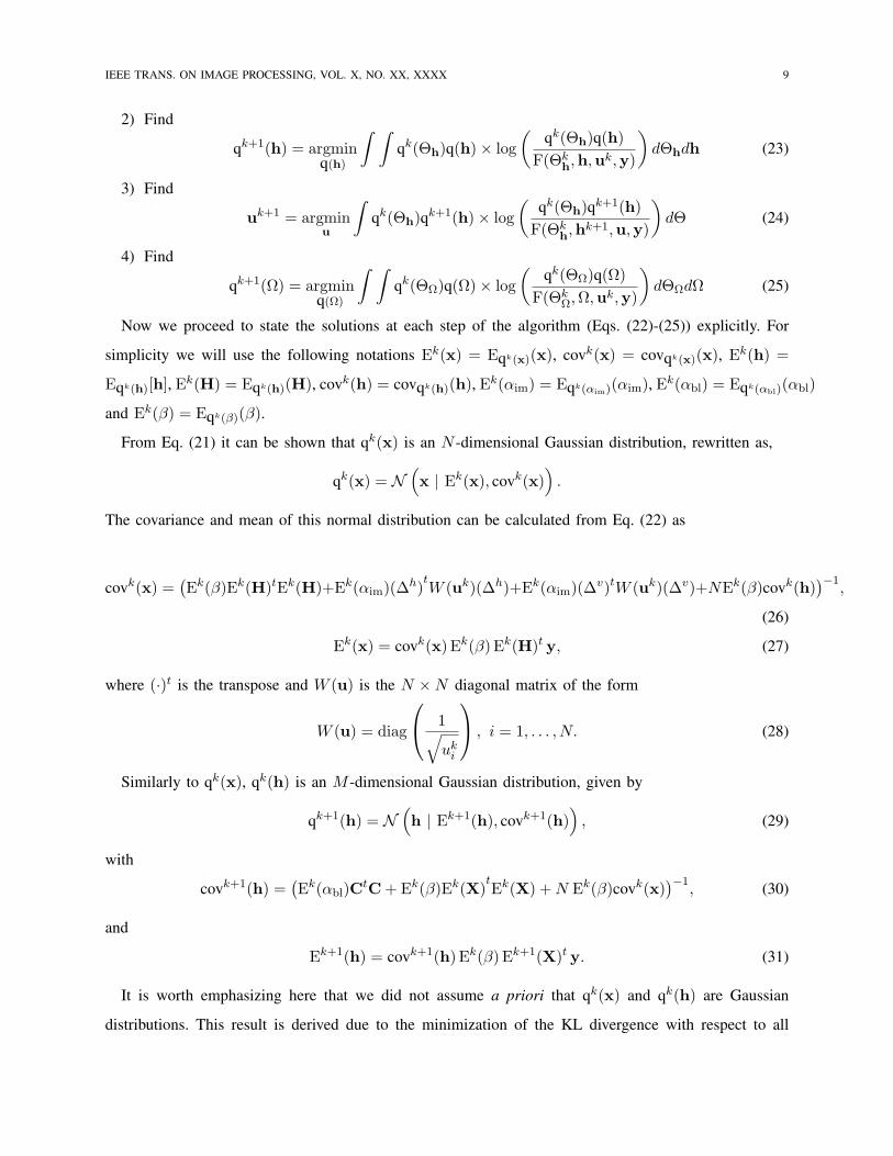
IEEE TRANS. ON IMAGE PROCESSING, VOL. X, NO. XX, XXXX 10
possible distributions according to the factorization q(Θ) = q(αim)q(αbl)q(β)q(x)q(h) [24]. Note also
that the image estimate in Eq. (27) is very similar to the image estimate proposed in [5] within a
regularization framework; the uncertainty term Nβkcovqk(h)[h] is missing however in [5]. As we will
see in the experimental results, this formulation will provide improved restoration results.
In step 4 of the algorithm, we find uk+1 from Eq. (24), given by
uk+1 = arg minu
∑i
Eqk(x)[(∆hi (x))2 + (∆v
i (x))2] + ui√ui
. (32)
Therefore, uk+1 can be obtained as
uk+1i = Eqk(x)[(∆
hi (x))2 + (∆v
i (x))2], i = 1, . . . , N, (33)
where
Eqk(x)[(∆hi (x))2 + (∆v
i (x))2] = (∆hi (Ek(x)))2 + ((∆v
i (Ek(x)))2
+ Eqk(x)[(∆hi (x− Ek(x)))2] + Eqk(x)[(∆
vi (x− Ek(x)))2], (34)
and
Eqk(x)[(∆hi (x− Ek(x)))2] + Eqk(x)[(∆
vi (x− Ek(x)))2] =
1N
trace[covk(x)×
((∆h)
t(∆h) + (∆v)t(∆v)
)].
(35)
It is clear that the vector uk+1 in Eq. (33) represents the local spatial activity of x using its distribution
approximation qk(x). Consequently, the matrix W (uk+1) in Eq. (28) is the spatial adaptivity matrix at
iteration k + 1 and it controls the smoothing applied to the unknown image in the restoration process.
For instance, at strong edges where the vector uk+1 has large values, W (uk+1) will have small values
so the amount of smoothing is decreased. On the other hand, in smooth regions the corresponding entry
of W (uk+1) will be very high, so smoothness is enforced. This property of the restoration is also in
accordance with the fact that noise is perceived as more visible in uniform regions than at edges (masking
effect of the human visual system). Note also that the spatial adaptivity matrix is also referred to as the
visibility matrix [25] and has been utilized in some image restoration approaches (see, for instance, [26]
and [27]).
After finding estimates of the posterior distributions of the image and blur, we find the estimates for
the hyperpriors at the last step of the algorithm. For ω ∈ αim, αbl, β, evaluating Eq. (25) using Eq. (21)
results in
qk+1(ω) ∝ exp Eqk(x)qk+1(h)q(Ωω)[log F(Ωkω, ω,x
k,hk+1,uk+1,y)].

IEEE TRANS. ON IMAGE PROCESSING, VOL. X, NO. XX, XXXX 11
Evaluating this explicitly we obtain
Eqk(x)qk+1(h) [log F(Θ) ] = const +∑
ω∈αim,αbl,β
((aoω − 1) logω − ω/boω)
+N
2logαim +
M
2logαbl +
N
2log β
− 12αimEqk(x)
∑i
(∆hi (x))2 + (∆v
i (x))2 + uk+1i√
uk+1i
− 1
2αblEqk+1(h)
[‖ Ch ‖2
]− 1
2βEqk(x)qk+1(h)
[‖ y −Hx ‖2
], (36)
where
Eqk(x)
∑i
(∆hi (x))2 + (∆v
i (x))2 + uk+1i√
uk+1i
= 2∑i
√uk+1i , (37)
Eqk+1(h)
[‖ Ch ‖2
]=‖ CEk+1(h) ‖2 +trace(CtC covk(h)), (38)
and
Eqk(x)qk+1(h)
[‖ y −Hx ‖2
]= ‖ y − Ek+1(h)Ek(x) ‖2 +trace(N covk(x) covk+1(h))
+ trace(Ek(X)t Ek(X) covk+1(h))
+ trace(Ek+1(H)t Ek+1(H) covk(x)). (39)
It can be seen from Eq. (36) that all hyperparameters have gamma distributions, given by
qk+1(αim) ∝ αN/2+aoαim
−1
im exp
[−αim(1/boαim
+∑i
√uk+1i )
], (40)
qk+1(αbl) ∝ αM/2+aoαbl
−1
bl exp
[−αbl(1/boαbl
+Eqk+1(h)
[‖ Ch ‖2
]2
], (41)
qk+1(β) ∝ βN/2+aoβ−1 exp
[−β(1/boβ +
Eqk(x)qk+1(h)
[‖ y −Hx ‖2
]2
)
], (42)
The means of these gamma distributions can be found using Eq. (10) and are represented as follows
(Ek+1(αim))−1 = γαim
1αoim
+ (1− γαim)
∑i
√uk+1i
N/2, (43)
(Ek+1(αbl))−1 = γαbl
1αobl
+ (1− γαbl)Eqk+1(h)
[‖ Ch ‖2
]M
, (44)
(Ek+1(β))−1 = γβ1βo + (1− γβ)
Eqk(x)qk+1(h)
[‖ y −Hx ‖2
]N
, (45)

IEEE TRANS. ON IMAGE PROCESSING, VOL. X, NO. XX, XXXX 12
where αoim = aoαim/boαim
, αbl = aoαbl/boαbl
and βo = aoβ/b
oβ and
γαim =aoαim
aoαim+ N
2
, γαbl =aoαbl
aoαbl+ M
2
, γβ =aoβ
aoβ + N2
. (46)
The parameters γαim , γαbl , and γβ can be understood as normalized confidence parameters, as can be
seen from Eqs. (43)-(46) and they take values in the interval [0, 1). Therefore, the means of the posterior
distributions of the hyperparameters are convex combinations of the prior hyperparameter values and their
maximum likelihood (ML) estimates. When the confidence parameters are asymptotically equal to zero
no confidence is placed on the initial values of the hyperparameters, and their ML estimates are used.
On the other hand, a value asymptotically equal to one will result in no update on the hyperparameters,
so that the algorithm will fully rely on the given initial parameters. In this case no estimation of the
hyperparameters is performed.
In Algorithm 1 no assumptions were imposed on the posterior approximations q(x) and q(h). We
can, however, assume that these distributions are degenerate, i.e., distributions which take one value with
probability one and the rest of the values with probability zero. We can obtain another algorithm under
this assumption which is similar to algorithm 1. In this second algorithm, the value of the KL divergence
is again decreased at each update step, but not by the maximum possible amount as was the case in
algorithm 1.
Utilizing the fact that the distributions on x and h are degenerate, that is,
q(x) = δ(x− x) =
1 if x = x
0 otherwise(47)
q(h) = δ(h− h) =
1 if h = h
0 otherwise(48)
with δ(·) the delta function, we obtain the following algorithm 2, where we use xk and hk to denote
the values qk(x) and qk(h) take with probability one, respectively, that is, qk(x) = δ(x − xk) and
qk(h) = δ(h− hk).
Algorithm 2: Given q1(h), q1(αim), q1(αbl), and q1(β) the initial estimates of the distributions q(h),
q(αim), q(αbl) and q(β), with q1(h) a degenerate distribution on h1,
for k = 1, 2, . . . until a stopping criterion is met:
1) Calculate
xk =(
Ek(β)(Hk)tHk + Ek(αim)(∆h)tW (uk)(∆h) + Ek(αim)(∆v)tW (uk)(∆v)
)−1
× Ek(β)(Hk)ty (49)
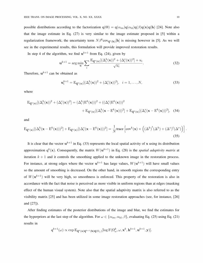
IEEE TRANS. ON IMAGE PROCESSING, VOL. X, NO. XX, XXXX 13
2) Calculate
hk =(
Ek(αbl)CtC + Ek(β)(Xk)tXk)−1
Ek(β)(Xk)tx (50)
3) Calculate
uk+1i = (∆h
i (xk))2 + (∆vi (x
k))2, i = 1, . . . , N. (51)
4) Calculate
qk+1(αim, αbl, β) = qk+1(αim)qk+1(αbl)qk+1(β), (52)
where qk+1(αim), qk+1(αbl) and qk+1(β) are gamma distributions given respectively by
qk+1(αim) ∝ αN/2+aoαim
−1
im exp
[−αim(1/boαim
+∑i
√uk+1i )
], (53)
qk+1(αbl) ∝ αM/2+aoαbl
−1
bl exp[−αbl(1/boαbl
+‖ Chk ‖2
2)], (54)
qk+1(β) ∝ βN/2+aoβ−1 exp[−β(1/boβ +
‖ y −Hkxk ‖2
2)]. (55)
Set
q(αim, αbl, β) = limk→∞
qk(αim, αbl, β), x = limk→∞
xk, h = limk→∞
hk. (56)
The update equations for the inverse of the means of the hyperparameters are then obtained from
Eqs. (53)-(55) as follows:
(Ek+1(αim))−1 = γαim
1αoim
+ (1− γαim)
∑i
√uk+1i
N/2, (57)
(Ek+1(αbl))−1 = γαbl
1αobl
+ (1− γαbl)‖ Chk ‖2
M, (58)
(Ek+1(β))−1 = γβ1βo + (1− γβ)
‖ y −Hkxk ‖2
N. (59)
It is clear that using degenerate distributions for x and h in Algorithm 2 removes the uncertainty terms
of the image and blur estimates. We will show in the experimental results section that these uncertainty
terms (the covariances of x and h) help to improve the restoration performance in high-noise cases,
where the image and blur estimates can be poor. The poor estimation of one variable can influence
the estimation of the other unknowns because of the alternating optimization procedure, and the overall
performance of the algorithm will be affected. By estimating the full posterior distribution instead of
the points corresponding to the maximum probability, the uncertainty of the estimates can be used to
IEEE TRANS. ON IMAGE PROCESSING, VOL. X, NO. XX, XXXX 14
ameliorate these effects in the estimation of the unknowns. On the other hand, at low-noise cases where
the estimates of the unknowns are more precise, Algorithm 2 results in better restorations.
Summarizing, Algorithm 1 iterates between Eqs. (27), (31), (33) and (43)-(45), whereas Algorithm 2
iterates between Eqs. (49), (50), (51) and (57)-(59) until convergence. Finally, a few remarks are needed
for the calculation of the image and blur estimates. The blur estimates in Eqs. (31) and (50) can be
calculated by assuming block circulant with circulant sub-matrices (BCCB) matrices for X and C, and
finding the solutions in the Fourier domain, which is very efficient [28]. However, finding closed form
solutions for the systems in Eqs. (27) and (49) is practically very difficult because the BCCB assumption
is not valid due to W, and the high dimensionality of the matrices makes it hard to find the inverses.
Therefore, we find numerical solutions by using a gradient descent (GD) algorithm which is very similar
to the one proposed in [26] with small modifications. Other numerical techniques, such as conjugate
gradient, can also be employed. Note that improved convergence and speed can be achieved by utilizing
preconditioning methods (see, for example, [29], [30]).
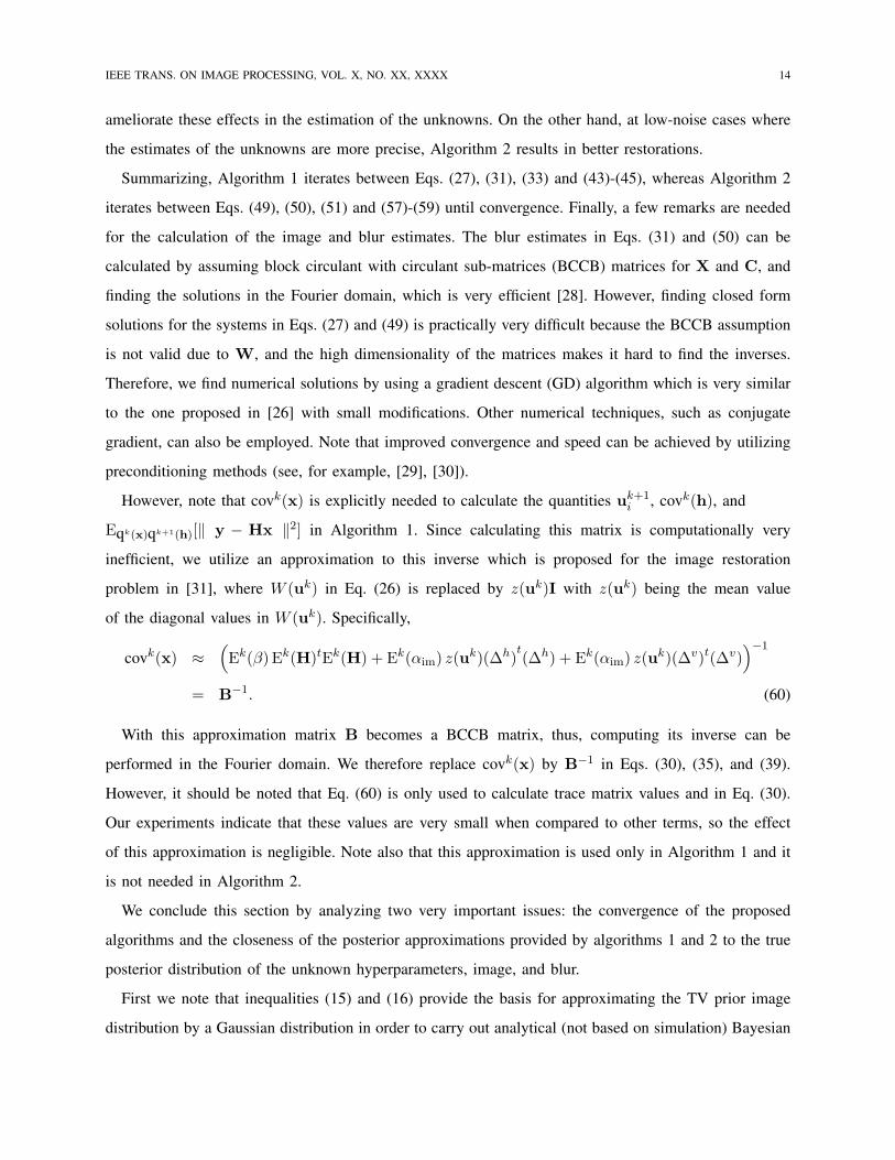
However, note that covk(x) is explicitly needed to calculate the quantities uk+1i , covk(h), and
Eqk(x)qk+1(h)[‖ y − Hx ‖2] in Algorithm 1. Since calculating this matrix is computationally very
inefficient, we utilize an approximation to this inverse which is proposed for the image restoration
problem in [31], where W (uk) in Eq. (26) is replaced by z(uk)I with z(uk) being the mean value
of the diagonal values in W (uk). Specifically,
covk(x) ≈(
Ek(β) Ek(H)tEk(H) + Ek(αim) z(uk)(∆h)t(∆h) + Ek(αim) z(uk)(∆v)t(∆v)
)−1
= B−1. (60)
With this approximation matrix B becomes a BCCB matrix, thus, computing its inverse can be
performed in the Fourier domain. We therefore replace covk(x) by B−1 in Eqs. (30), (35), and (39).
However, it should be noted that Eq. (60) is only used to calculate trace matrix values and in Eq. (30).
Our experiments indicate that these values are very small when compared to other terms, so the effect
of this approximation is negligible. Note also that this approximation is used only in Algorithm 1 and it
is not needed in Algorithm 2.
We conclude this section by analyzing two very important issues: the convergence of the proposed
algorithms and the closeness of the posterior approximations provided by algorithms 1 and 2 to the true
posterior distribution of the unknown hyperparameters, image, and blur.
First we note that inequalities (15) and (16) provide the basis for approximating the TV prior image
distribution by a Gaussian distribution in order to carry out analytical (not based on simulation) Bayesian

IEEE TRANS. ON IMAGE PROCESSING, VOL. X, NO. XX, XXXX 15
analysis. From Eq. (19) we have that
M(q(Θ)) ≤ M(q(Θ),u) , (61)
and so algorithms 1 and 2 provide a sequence of distributions qk(Θ) and a sequence of vectors uk
that satisfy
M(qk(Θ),uk) ≥ M(qk(Θ),uk+1) ≥ M(qk+1(Θ),uk+1). (62)
Notice that when we decrease the value of the posterior approximation M(q(Θ),uk+1) we obtain qk+1(Θ)
which provides a decreased upper bound of M(qk+1(Θ)). Furthermore, minimizing M(qk(Θ),u) with
respect to u generates a new vector uk that tightens the upper-bound of M(qk(Θ)). Consequently,
algorithms 1 and 2 provide sequences of ever decreasing upper bounds. These sequences are bounded
from below by − log p(y) (see Eq. (13)) and consequently they converge.
Let us now examine the quality of the estimated posterior distributions. We only analyze here the type
of the posterior distribution approximation obtained by algorithm 1; the discussion about algorithm 2
is very similar since in the iterative procedure we only use the mean and do not take into account its
uncertainty. Inequality (15) provides a local quadratic approximation to the TV prior. Using always uo
with all its entries being equal is equivalent to utilizing a fixed global conditional auto-regression model
to approximate the TV image prior. Clearly, the procedure which updates u (even if all its components
are the same) will provide a tighter upper bound for M(q(Θ)).
Let us also comment on the proximity of the estimated posterior distributions to the true posteriors.
By using a different majorization of TV (x) from the one used in inequality (15) we obtain different
approximations of the TV image prior. A major advantage of the one used in the paper is that it results
in a quadratic approximation which is easy to analyze analytically. The closeness of the variational
approximation to the true posterior in two or more dimensions is still an open question. Notice, however,
that we have proved the optimality, in the divergence sense, of the obtained approximation among a given
class of Gaussian distributions. Insightful comments on when the variational approximation may be tight
can be found in [32] (see also [33] and [34]). A discussion on approximate Bayesian inference using
variational methods and its comparison with other bounds can be found in [20].
IV. EXPERIMENTAL RESULTS
In this section we present both synthetic and real blind deconvolution examples to demonstrate the
performance of the algorithms. In the results reported below, we will denote Algorithm 1 by TV1, and
Algorithm 2, where the distributions q(x) and q(h) are both degenerate, by TV2. We compare our

IEEE TRANS. ON IMAGE PROCESSING, VOL. X, NO. XX, XXXX 16
(a) (b) (c)
(d) (e) (f)
Fig. 2. (a) Lena image; degraded with a Gaussian shaped PSF with variance 9 and Gaussian noise of variance: (b) 0.16 (BSNR
= 40 dB), (c) 16 (BSNR = 20 dB), (d) Shepp-Logan phantom; degraded with a Gaussian shaped PSF with variance 9 and
Gaussian noise of variance: (e) 0.18 (BSNR = 40 dB), (f) 18 (BSNR = 20 dB).
algorithms with two other blind deconvolution algorithms based on variational approximations proposed
in [7], which use SAR models for both the image and the blur. These algorithms are denoted by SAR1 and
SAR2, where SAR1 provides an approximation to the full posterior distribution of the image and the blur,
and SAR2 assumes degenerate distributions. Comparing the proposed algorithms with SAR1 and SAR2
provides a measure of the effectiveness of the proposed TV image prior, and also the performance of the
spatially adaptive deconvolution compared to nonspatially adaptive restoration methods. In the synthetic
experiments we also include the results from the non-blind versions of our algorithms, where the blur is
assumed to be known and only the image and the hyperparameters are estimated during iterations. These
non-blind algorithms will be denoted as TV1-NB and TV2-NB.
For the first set of our experiments, “Lena”, “Cameraman” and “Shepp-Logan” phantom images are
blurred with a Gaussian-shaped function with variance 9, and white Gaussian noise is added to obtain

IEEE TRANS. ON IMAGE PROCESSING, VOL. X, NO. XX, XXXX 17
degraded images with blurred-signal-to-noise ratios (BSNR) of 20dB and 40dB. The original and degraded
“Lena” images and “Shepp-Logan” phantoms are shown in Fig. 2. The initial values for the TV1 and
TV2 algorithms are chosen as follows: The observed image y is used as the initial estimate of x1,
and a Gaussian function with variance 4 as the initial estimate h1 of the blur. The covariance matrices
cov1(h) and cov1(x) are set equal to zero. The initial values β1, α1im, and α1
bl are calculated according
to Eqs. (43)–(45), assuming degenerate distributions, and the initial value u1 is calculated using x1
in Eq. (51). It should be emphasized that except from the initial value of the blur, all parameters are
automatically estimated from the observed image. For the SAR1 and SAR2 algorithms, the same initial
blur is used, and other parameters are calculated also automatically from the observed image [7].
In this first set of experiments, we set all confidence parameters equal to zero, i.e., the observation is
made fully responsible for the estimation process. The quantitative results are shown in Table I, where
ISNR is defined as 10 log10(‖ x−y ‖2 / ‖ x− x ‖2), where x, y, and x represent the original, observed,
and estimated images, respectively. For all experiments, ‖ xk − xk−1 ‖2 / ‖ xk−1 ‖2< 10−5 (or Ek(x)
instead of xk) is used to terminate the algorithms, and a threshold of 10−5 is used to terminate the GD
iterations. The corresponding restoration results for the “Lena” image are shown in Fig. 3 for the 40 dB
BSNR case, and in Fig. 4 for the 20 dB BSNR case.
A few remarks can be made by examining the ISNR values in Table I and the restorations visually.
First, note that the non-blind algorithms TV1-NB and TV2-NB result in higher ISNR values than the blind
ones, as expected, although the resulting images are visually comparable. Secondly, algorithms TV1 and
TV2 result in higher ISNR values for all images and noise levels than the SAR-based algorithms. Visually,
the TV-based algorithms result in sharper restorations, and in addition the ringing artifacts are reduced.
Another important point is that algorithms TV2 and SAR2 fail to converge to successful restorations for
the 20 dB BSNR case. On the other hand, algorithms TV1 and SAR1 result in acceptable restorations in
this case. As can be seen in Figs. 4(a), (c) TV1 succeeds at removing the blur and reducing the ringing
artifacts providing a better restored image than the SAR1 algorithm.
The differences between the TV-based and SAR-based algorithms are clearer in the restoration of the
Shepp-Logan phantom, which are shown in Fig. 5 for the 40 dB BSNR case, and in Fig. 6 for the 20 dB
BSNR case. Algorithms TV1 and TV2 clearly outperform the SAR algorithms in terms of preserving and
recovering the edges, whereas the ringing artifacts are more visible at 40 dB BSNR than at 20dB BSNR.
Again, algorithms TV2 and SAR2 fail to converge to meaningful restorations for the 20 dB BSNR case.
Note that in other cases the restorations by TV1 and TV2 are very close to non-blind restoration results,
except for some ringing artifacts resulting from estimation errors in the PSF.

IEEE TRANS. ON IMAGE PROCESSING, VOL. X, NO. XX, XXXX 18
TABLE I
ISNR VALUES AND NUMBER OF ITERATIONS FOR THE LENA, CAMERAMAN AND SHEPP-LOGAN IMAGES DEGRADED BY A
GAUSSIAN BLUR WITH VARIANCE 9.
Lena Cameraman Shepp-Logan
BSNR Method ISNR (dB) iterations ISNR (dB) iterations ISNR (dB) iterations
40dB TV1 2.53 85 1.82 92 3.07 200
TV2 2.95 200 1.73 200 3.36 200
SAR1 1.35 63 1.03 66 1.20 121
SAR2 1.43 78 1.01 89 1.35 180
TV1-NB 4.33 9 2.96 11 4.16 28
TV2-NB 4.31 9 2.95 11 4.15 28
20dB TV1 2.62 81 1.70 5 2.47 8
TV2 -32.50 500 -40.89 392 -23.88 476
SAR1 1.62 80 1.16 98 1.53 146
SAR2 -11.32 54 -8.83 80 -6.59 29
TV1-NB 3.31 11 2.42 12 4.28 17
TV2-NB 3.29 11 2.41 12 4.27 17
A possible reason that algorithms TV2 and SAR2 fail to provide meaningful restorations for the 20 dB
BSNR case is the lack of the uncertainty terms covk(h) and covk(x) in Eqs. (49) and (50), respectively.
In this case, the matrices that are inverted in Eqs. (49)-(50) become worse conditioned than the matrices
being inverted in algorithms TV1 (in Eqs. (26) and (30)) and SAR1, thus degrading the quality of the
restorations.
We note here that the proposed algorithms are quite robust to the initial selected value of the blur.
When a Gaussian with variance 2 is chosen as h1, the ISNR values are 1.80 dB for TV1 and 2.75 dB
for TV2 for 40 dB BSNR, and 1.71 for TV1 and -33.36 dB for TV2 for 20 dB BSNR, similarly to the
results in Table I.
One dimensional slices through the origin of the estimated blurs for all algorithms corresponding to
the restoration of the ”Lena” image are shown in Fig. 7. It is clear that all algorithms provide accurate
estimates of the true PSF for both noise levels. As already mentioned, TV2 and SAR2 fail to converge to
meaningful PSF and image estimates at 20 dB BSNR.
Before proceeding with the next set of experiments, we compare the SAR blur prior with the TV
prior on the blur, as used in [5]. The algorithms proposed in [5] and [15] place TV priors both on the
unknown image and blur and follow a regularization-based restoration procedure to estimate them. The
IEEE TRANS. ON IMAGE PROCESSING, VOL. X, NO. XX, XXXX 19
(a) (b) (c)
(d) (e) (f)
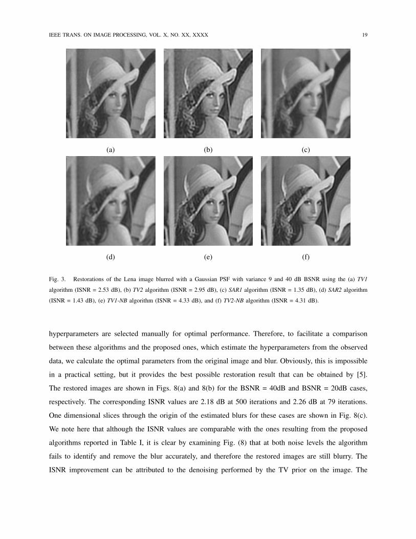
Fig. 3. Restorations of the Lena image blurred with a Gaussian PSF with variance 9 and 40 dB BSNR using the (a) TV1
algorithm (ISNR = 2.53 dB), (b) TV2 algorithm (ISNR = 2.95 dB), (c) SAR1 algorithm (ISNR = 1.35 dB), (d) SAR2 algorithm
(ISNR = 1.43 dB), (e) TV1-NB algorithm (ISNR = 4.33 dB), and (f) TV2-NB algorithm (ISNR = 4.31 dB).
hyperparameters are selected manually for optimal performance. Therefore, to facilitate a comparison
between these algorithms and the proposed ones, which estimate the hyperparameters from the observed
data, we calculate the optimal parameters from the original image and blur. Obviously, this is impossible
in a practical setting, but it provides the best possible restoration result that can be obtained by [5].
The restored images are shown in Figs. 8(a) and 8(b) for the BSNR = 40dB and BSNR = 20dB cases,
respectively. The corresponding ISNR values are 2.18 dB at 500 iterations and 2.26 dB at 79 iterations.
One dimensional slices through the origin of the estimated blurs for these cases are shown in Fig. 8(c).
We note here that although the ISNR values are comparable with the ones resulting from the proposed
algorithms reported in Table I, it is clear by examining Fig. (8) that at both noise levels the algorithm
fails to identify and remove the blur accurately, and therefore the restored images are still blurry. The
ISNR improvement can be attributed to the denoising performed by the TV prior on the image. The

IEEE TRANS. ON IMAGE PROCESSING, VOL. X, NO. XX, XXXX 20
(a) (b) (c)
(d) (e) (f)
Fig. 4. Restorations of the Lena image blurred with a Gaussian PSF with variance 9 and 20 dB BSNR using the (a) TV1
algorithm (ISNR = 2.62 dB), (b) TV2 algorithm (ISNR = -32.50 dB), (c) SAR1 algorithm (ISNR = 1.62 dB), (d) SAR2 algorithm
(ISNR = -11.32 dB), (e) TV1-NB algorithm (ISNR = 3.31 dB), and (f) TV2-NB algorithm (ISNR = 3.29 dB).
convergence is extremely slow in the BSNR = 40 dB case. In the BSNR = 20 dB case, the estimated PSF
is very similar to an out-of-focus blur, indicating that the algorithm fails to identify the smooth nature
of the PSF. These results are also in agreement with the ones reported in [5]. Based on the above, it is
reasonable to conclude that for smooth PSFs such as a Gaussian, the proposed algorithms with the SAR
blur prior outperform algorithms utilizing a TV blur prior, given also the fact that all required parameters
are calculated from the observed image in an automated fashion.
In the second set of experiments, we tested the algorithms with a less severe blur. The images are blurred
with a Gaussian shaped PSF with variance 5, and the initial estimate of the blur, h1, is a Gaussian PSF
with variance 2. The corresponding ISNR values of the restorations are shown in Table II. As expected,
all algorithms provide better restorations in this case, although the noise variances are higher compared
to the first set of experiments to obtain the same BSNRs. Similarly to the first experiment, algorithms

IEEE TRANS. ON IMAGE PROCESSING, VOL. X, NO. XX, XXXX 21
(a) (b) (c)
(d) (e) (f)
Fig. 5. Restorations of the Shepp-Logan phantom blurred with a Gaussian PSF with variance 9 and 40 dB BSNR using the
(a) TV1 algorithm (ISNR = 3.07 dB), (b) TV2 algorithm (ISNR = 3.36 dB), (c) SAR1 algorithm (ISNR = 1.20 dB), (d) SAR2
algorithm (ISNR = 1.35 dB), (e) TV1-NB algorithm (ISNR = 4.16 dB), and (f) TV2-NB algorithm (ISNR = 4.15 dB).
TV1 and TV2 result in better restoration performance both in terms of ISNR and visual quality.
Before proceeding with the next experiment, an important observation has to be made. We noticed in
our experiments that the quality of the estimation of u is a very important factor in the performance of the
algorithms. For example, in the case of “Lena” with BSNR = 40 dB and Gaussian PSF with variance 5,
if we run the algorithms TV1 and TV2 by calculating u from the original image, we obtain ISNR values
of 3.52 dB and 3.60 dB, respectively. Other cases showed similar improvements. Thus knowledge about
this parameter greatly improves the ISNR performance (a similar conclusion is drawn in [26], [31]). This
also confirms that the decrease in the performance of the algorithms in the presence of high noise, e.g.,
BSNR = 20dB, is due to the fact that the spatial variations in the image, hence the parameter u, cannot be
estimated well. This is also observed in [35] and several solutions are proposed for TV image restoration.
In this work, we adapted a simple smoothing of the gradient of the image with a small Gaussian PSF
(with variance 1) which largely improves both the performance and the convergence of the algorithms.
IEEE TRANS. ON IMAGE PROCESSING, VOL. X, NO. XX, XXXX 22
(a) (b) (c)
(d) (e) (f)
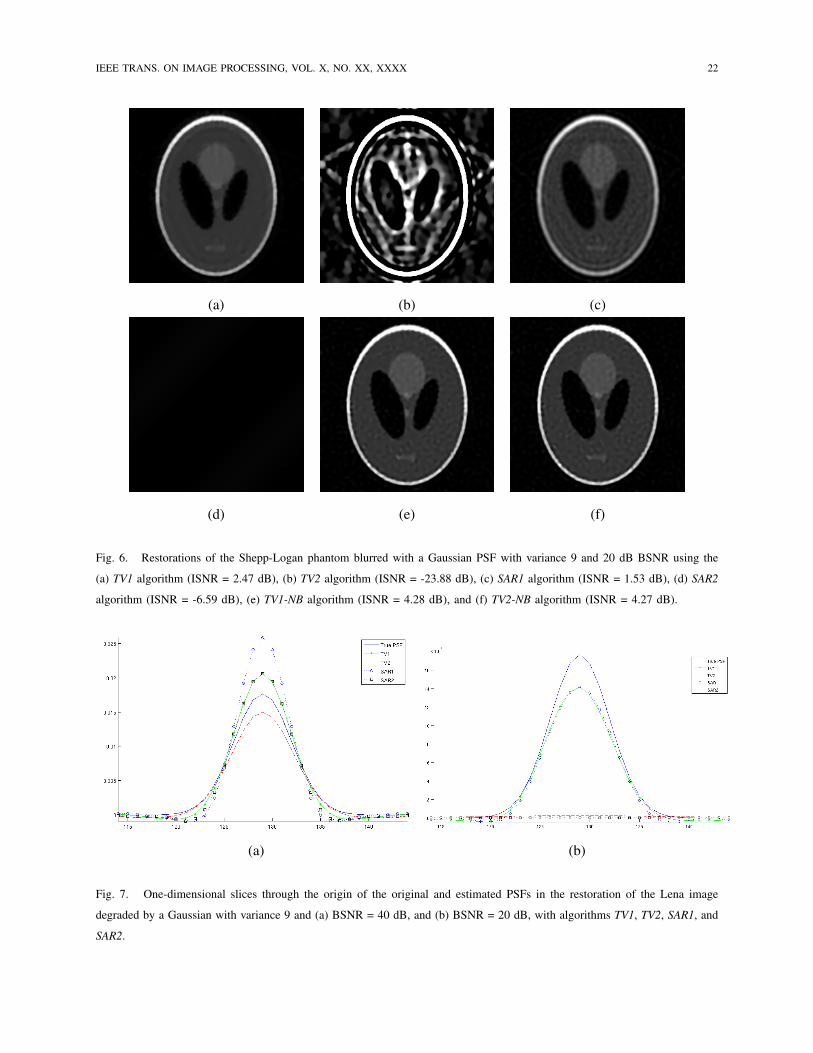
Fig. 6. Restorations of the Shepp-Logan phantom blurred with a Gaussian PSF with variance 9 and 20 dB BSNR using the
(a) TV1 algorithm (ISNR = 2.47 dB), (b) TV2 algorithm (ISNR = -23.88 dB), (c) SAR1 algorithm (ISNR = 1.53 dB), (d) SAR2
algorithm (ISNR = -6.59 dB), (e) TV1-NB algorithm (ISNR = 4.28 dB), and (f) TV2-NB algorithm (ISNR = 4.27 dB).
(a) (b)
Fig. 7. One-dimensional slices through the origin of the original and estimated PSFs in the restoration of the Lena image
degraded by a Gaussian with variance 9 and (a) BSNR = 40 dB, and (b) BSNR = 20 dB, with algorithms TV1, TV2, SAR1, and
SAR2.

IEEE TRANS. ON IMAGE PROCESSING, VOL. X, NO. XX, XXXX 23
(a) (b)
(c)
Fig. 8. Restorations of the Lena image blurred with a Gaussian PSF with variance 9 using a TV blur prior and fixed optimal
parameters as in [5]. (a) Restoration at 40 dB BSNR (ISNR = 2.18 dB), (b) restoration at 20 dB BSNR (ISNR = 2.26 dB), (c)
estimated blur PSFs.
Therefore, it is safe to claim that in high noise-cases, incorporating robust gradient estimation methods,
such as [35], [36], will further improve the performance of the proposed algorithms.
We now examine the effect of prior information on the performance of the proposed algorithms in
the third set of experiments. Generally, some information about the values of the hyperparameters is
available and can be utilized in the restoration to improve performance. For instance, the noise variance
can be estimated quite accurately when a part of the image has uniform color. The image variance is
more difficult to estimate from a single degraded observation. However, a set of images with similar
characteristics can be used to acquire an estimate for this parameter. If an estimate of the image variance
can be provided, the PSF variance can be approximated using this value (see [37] for details).
In addition to the prior knowledge on the hyperparameters, constraints on the blur estimates can also
be imposed. Positivity and symmetry constraints are the most common ones, and it is known that they

IEEE TRANS. ON IMAGE PROCESSING, VOL. X, NO. XX, XXXX 24
TABLE II
ISNR VALUES AND NUMBER OF ITERATIONS FOR THE LENA, CAMERAMAN AND SHEPP-LOGAN IMAGES DEGRADED BY A
GAUSSIAN BLUR WITH VARIANCE 5.
Lena Cameraman Shepp-Logan
BSNR Method ISNR (dB) iterations ISNR (dB) iterations ISNR (dB) iterations
40dB TV1 3.19 200 1.66 73 2.05 137
TV2 3.29 115 2.49 58 3.79 200
SAR1 1.26 53 0.90 53 1.24 157
SAR2 1.45 77 0.99 86 1.51 200
TV1-NB 4.98 10 3.50 12 7.57 43
TV2-NB 4.93 10 3.48 12 7.29 39
20dB TV1 1.39 189 1.43 136 2.09 200
TV2 -45.20 436 -42.54 297 -26.00 478
SAR1 1.14 87 0.87 76 1.24 200
SAR2 -13.15 55 -10.02 73 -7.87 27
TV1-NB 2.92 10 2.40 12 4.68 16
TV2-NB 2.83 11 2.37 12 4.65 16
can significantly improve the convergence of the algorithms and the quality of the estimates [5]. Although
such hard constraints have not been directly incorporated in our Bayesian framework, they can in practice
improve the restoration results of the proposed algorithms TV1 and TV2 as shown experimentally next.
For simulation purposes, we calculated the values of the hyperparameters from the original image and
PSF to be used as prior hyperparameter values. Then, using these prior values, we applied TV1 to the
“Lena” image degraded by a Gaussian PSF and 40 dB BSNR with varying confidence parameters and
obtained the ISNR evolution graphs shown in Fig. 9. To show the improved restoration performance
and the best achievable ISNR, we applied positivity and symmetry constraints to the estimated PSF at
each iteration as in [5]. Additionally, the support of the blur is estimated at each iteration using the first
zero-crossing of the PSF from its center, and values outside this estimated support are set equal to zero.
Selected ISNR values from these graphs with the estimated hyperparameters are shown in Table III. We
included cases corresponding to the best ISNR values when (a) information about the noise variance is
available, (b) information about only the PSF variance is available, (c) information about only the image
variance is available, and (d) information about all hyperparameters is available. It is clear that if some
information on the hyperparameters is available, biasing the algorithm towards these hyperparameters

IEEE TRANS. ON IMAGE PROCESSING, VOL. X, NO. XX, XXXX 25
(a) (b)
(c) (d)
Fig. 9. ISNR evolution for different values of the confidence parameters for Algorithm 1 (TV1) applied to the “Lena” image
degraded by a Gaussian with variance 9 and BSNR = 40 dB. (a) For fixed γβ = 0, (b) for fixed γαbl = 0, (c) for fixed γαim = 0,
and (d) for fixed γβ = 1.
leads to improved ISNR values. However, it is interesting that incorporating the knowledge about the
true value of the noise variance decreases the quality of the restorations, thus, it is better to put no
confidence on this parameter and let the algorithms adaptively select it at each iteration. On the other
hand, we note that at convergence, the Ek(β)−1 almost always converged to a value very close to the
noise variance.
It should also be emphasized that the most critical hyperparameter is αbl. It is clear from Fig. 9 and
Table III that incorporating information about this parameter greatly increases the performance of the
algorithm, and that the best ISNR is achieved when γαbl = 1 is used. Restoration results with these
confidence parameters are shown in Fig. 10. Note that the restoration quality is almost as high as the
one achieved by the non-blind algorithms (see Fig.3(e) for comparison). One dimensional slices of the
estimated blurs corresponding to these cases are shown in Fig. 11, where it can be seen that the estimated

IEEE TRANS. ON IMAGE PROCESSING, VOL. X, NO. XX, XXXX 26
TABLE III
POSTERIOR MEANS OF THE DISTRIBUTIONS OF THE HYPERPARAMETERS, ISNR, AND NUMBER OF ITERATIONS USING TV1
FOR THE LENA IMAGE WITH 40 DB BSNR USING αimo = 0.042, αbl
o = 4.6× 10⁸ , AND βo
= 6.25, FOR DIFFERENT
VALUES OF γαim , γαim AND γβ .
γαim γαbl γβ E[αim] E[αbl] E[β] ISNR (dB) iterations
0 0 0 0.088 3.3× 10⁸ 5.63 3.65 32
0 1 0 0.086 4.6× 10⁸ 5.62 3.85 38
1 1 0 0.041 4.6× 10⁸ 5.75 3.90 51
1 0 0 0.041 3.7× 10⁸ 5.76 3.80 51
0.6 1 0 0.051 4.6× 10⁸ 5.72 3.92 45
0.8 1 1 0.046 4.6× 10⁸ 6.25 3.80 82
(a) (b) (c) (d)
Fig. 10. Some restorations of the Lena image blurred with a Gaussian PSF with variance 9 and 40 dB BSNR using the TV1
algorithm utilizing prior knowledge through confidence parameters and positivity and support constraints on the estimated blur.
(a) γαim = γαbl = γβ = 0.0 (ISNR = 3.65 dB), (b) γαim = 0, γαbl = 1, γβ = 0 (ISNR = 3.85 dB), (c) γαim = 0.6, γαbl = 1,
γβ = 0 (ISNR = 3.92 dB), and (d) γαim = 0.8, γαbl = 1, γβ = 1 (ISNR = 3.80 dB).
PSFs are much closer to the true PSF than the ones in Fig. 7. Overall, it is clear from the results that,
as expected, the performance of the algorithms can be largely increased when some information about
these hyperparameters is provided and certain constraints on the estimated blur are imposed.
In our last set of experiments, the algorithms are applied to a real image of Saturn, which was taken
at the Calar Alto Observatory in Spain, shown in Fig. 12(a). There is no exact expression the shape of
the PSF for this image, however, the following approximation is suggested in [38], [39]
h(r) ∝ (1 +r2
R2)−δ, (63)
with δ = 3 and R = 3.4. The non-blind restoration result using TV2-NB with this theoretical PSF is
shown in Fig. 12(b). This image is restored first by TV1 and TV2 with zero confidences placed on the prior

IEEE TRANS. ON IMAGE PROCESSING, VOL. X, NO. XX, XXXX 27
Fig. 11. One-dimensional slices through the origin of the original and estimated PSFs in the restoration of the Lena image
degraded by a Gaussian with variance 9 and BSNR = 40dB with algorithm TV1. (a) True PSF, Estimated PSF with (b) γαim =
γαbl = γβ = 0.0, (c) γαim = 0, γαbl = 1, γβ = 0, (d) γαim = 0.6, γαbl = 1, γβ = 0, and (e) γαim = 0.8, γαbl = 1, γβ = 1.
values, i.e., γαim = γαbl = γβ = 0. The initial blur is selected as a Gaussian shaped PSF with variance 1.
Our experiments show that TV2 gives a reasonably good restoration result, shown in Fig. 12(c), whereas
TV1 does not adequately remove the blur.
However, as in the previous experiment, the quality of the restorations can be improved by utilizing
prior knowledge about the parameters. We used βo = 8.16, αoim = 0.24, and αobl = 1.6 × 10⁸ as prior
hyperparameter values, which are obtained by running TV2-NB with the PSF in Eq. (63). By selecting
γαim = 0.8, γαbl = 0.1, and γβ = 0.8, we obtain the restorations shown in Fig. 12(d) with TV1
and Fig. 12(d) with TV2. As a comparison, the restoration result with SAR1 with the same confidence
parameters is shown in Fig. 12(e). Note that TV-based approaches are more successful at removing the
blur while providing smooth restorations with less ringing. The estimated PSFs corresponding to these
cases as well as the theoretical PSF is shown in Fig. (13). It is clear that the estimated PSFs by the
proposed algorithms are much closer to the theoretical PSF than the SAR1 result, even when no prior
knowledge is incorporated.
We conclude this section by commenting on the computational complexity of the algorithms. The pro-
posed algorithms are computationally more intensive than SAR-based restoration methods since Eqs. (27)
and (49) cannot be solved by direct inversion in the frequency domain and iterative numerical approaches
are needed. Typically, the MATLAB implementations of our algorithms required on the average about
20 seconds per iteration on a 3.20 GHz Xeon PC for 256x256 images. Note that the running time of
the algorithms can be improved by utilizing preconditioning methods (see, for example, [29] [30]), or
IEEE TRANS. ON IMAGE PROCESSING, VOL. X, NO. XX, XXXX 28
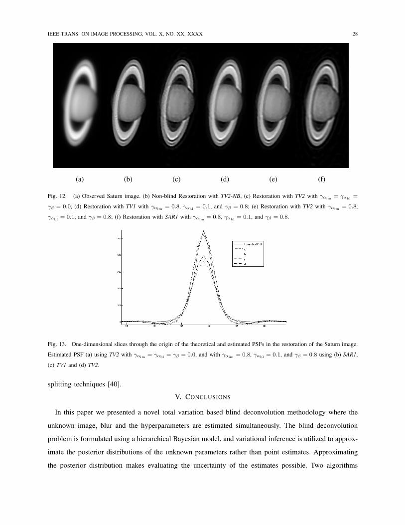
(a) (b) (c) (d) (e) (f)
Fig. 12. (a) Observed Saturn image. (b) Non-blind Restoration with TV2-NB, (c) Restoration with TV2 with γαim = γαbl =
γβ = 0.0, (d) Restoration with TV1 with γαim = 0.8, γαbl = 0.1, and γβ = 0.8; (e) Restoration with TV2 with γαim = 0.8,
γαbl = 0.1, and γβ = 0.8; (f) Restoration with SAR1 with γαim = 0.8, γαbl = 0.1, and γβ = 0.8.
Fig. 13. One-dimensional slices through the origin of the theoretical and estimated PSFs in the restoration of the Saturn image.
Estimated PSF (a) using TV2 with γαim = γαbl = γβ = 0.0, and with γαim = 0.8, γαbl = 0.1, and γβ = 0.8 using (b) SAR1,
(c) TV1 and (d) TV2.
splitting techniques [40].
V. CONCLUSIONS
In this paper we presented a novel total variation based blind deconvolution methodology where the
unknown image, blur and the hyperparameters are estimated simultaneously. The blind deconvolution
problem is formulated using a hierarchical Bayesian model, and variational inference is utilized to approx-
imate the posterior distributions of the unknown parameters rather than point estimates. Approximating
the posterior distribution makes evaluating the uncertainty of the estimates possible. Two algorithms

IEEE TRANS. ON IMAGE PROCESSING, VOL. X, NO. XX, XXXX 29
are provided resulting from this approach. It is shown that the unknown parameters of the Bayesian
formulation can be calculated automatically using only the observation or using also prior knowledge
with different confidence values to improve the performance of the algorithms. Experimental results
demonstrated that the proposed approaches result in high-quality restorations in both synthetic and real
image experiments.REFERENCES
[1] S. D. Babacan, R. Molina, and A. K. Katsaggelos, “Total variation blind deconvolution using a variational approach to
parameter, image, and blur estimation,” in EUSIPCO, Poznan, Poland, Sept. 2007.
[2] D. Kundur and D. Hatzinakos, “Blind image deconvolution,” IEEE Signal Processing Mag., vol. 13, no. 3, pp. 43–64,
1996.
[3] T. E. Bishop, S. D. Babacan, B. Amizic, A. K. Katsaggelos, T. Chan, and R. Molina, “Blind image deconvolution: problem
formulation and existing approaches,” in Blind image deconvolution: theory and applications, P. Campisi and K. Egiazarian,
Eds. CRC press, 2007, ch. 1.
[4] R. Fergus, B. Singh, A. Hertzmann, S. T. Roweis, and W. Freeman, “Removing camera shake from a single photograph,”
ACM Transactions on Graphics, SIGGRAPH 2006 Conference Proceedings, Boston, MA, vol. 25, pp. 787–794, 2006.
[5] T. F. Chan and C.-K. Wong, “Total variation blind deconvolution,” IEEE Trans. Image Processing, vol. 7, no. 3, pp.
370–375, Mar. 1998.
[6] A. C. Likas and N. P. Galatsanos, “A variational approach for Bayesian blind image deconvolution,” IEEE Trans. Signal
Processing, vol. 52, no. 8, pp. 2222–2233, 2004.
[7] R. Molina, J. Mateos, and A. K. Katsaggelos, “Blind deconvolution using a variational approach to parameter, image, and
blur estimation,” IEEE Trans. Image Processing, vol. 15, no. 12, pp. 3715–3727, Dec. 2006.
[8] J. H. Money and S. H. Kang, “Total variation minimizing blind deconvolution with shock filter reference,” Image Vision
Comput., vol. 26, no. 2, pp. 302–314, 2008.
[9] L. Bar, N. Sochen, and N. Kiryati, “Variational pairing of image segmentation and blind restoration,” in Proc. 8th European
Conference on Computer Vision (ECCV’2004), vol. Part II, LNCS 3022, Prague, Czech Republic, May 2004, pp. 166–177.
[10] M. Bronstein, A. Bronstein, M. Zibulevsky, and Y. Zeevi, “Blind deconvolution of images using optimal sparse
representations,” IEEE Trans. Image Processing, vol. 14, no. 6, pp. 726–736, June 2005.
[11] M. S. C. Almeida and L. B. Almeida, “Blind deblurring of natural images,” in ICASSP 2008, Las Vegas, USA, April 2008.
[12] S. Kullback, Information Theory and Statistics. New York, Dover Publications, 1959.
[13] J. W. Miskin and D. J. C. MacKay, “Ensemble learning for blind image separation and deconvolution,” in Advances in
Independent Component Analysis, M. Girolami, Ed. Springer-Verlag Scientific Publishers, July 2000.
[14] K. Z. Adami, “Variational methods in Bayesian deconvolution,” PHYSTAT2003 ECONF, vol. C030908, p. TUGT002, 2003.
[15] Y. L. You and M. Kaveh, “Blind image restoration by anisotropic regularization,” IEEE Trans. Image Processing, vol. 8,
no. 3, pp. 396–407, 1999.
[16] L. I. Rudin, S. Osher, and E. Fatemi, “Nonlinear total variation based noise removal algorithms,” Physica D, pp. 259–268,
1992.
[17] J. Bernardo and A. Smith, Bayesian Theory. New York: John Wiley and Sons, 1994.
[18] J. Bioucas-Dias, M. Figueiredo, and J. Oliveira, “Adaptive total-variation image deconvolution: A majorization-minimization
approach,” in Proceedings of EUSIPCO’2006, Florence, Italy, Sept. 2006.

IEEE TRANS. ON IMAGE PROCESSING, VOL. X, NO. XX, XXXX 30
[19] J. O. Berger, Statistical Decision Theory and Bayesian Analysis. New York, Springer Verlag, 1985, ch. 3 and 4.
[20] M. Beal, “Variational algorithms for approximate Bayesian inference,” Ph.D. dissertation, The Gatsby Computational
Neuroscience Unit, University College London, 2003.
[21] S. Kullback and R. A. Leibler, “On information and sufficiency,” Annals of Mathematical Statistics, vol. 22, pp. 79–86,
1951.
[22] G. Parisi, Statistical Field Theory. Redwood City, CA: Addison-Wesley, 1988.
[23] J. Miskin, “Ensemble learning for independent component analysis,” Ph.D. dissertation, Astrophysics Group, University of
Cambridge, 2000.
[24] C. M. Bishop, Pattern Recognition and Machine Learning. Springer-Verlag, 2006.
[25] G. L. Anderson and A. N. Netravali, “Image restoration based on a subjective criterion,” IEEE Trans. Syst., Man, Cybern.
6, pp. 845–853, 1976.
[26] S. D. Babacan, R. Molina, and A. Katsaggelos, “Parameter estimation in TV image restoration using variational distribution
approximation,” IEEE Trans. Image Processing, no. 3, pp. 326–339, 2008.
[27] A. K. Katsaggelos and M. G. Kang, “A spatially adaptive iterative algorithm for the restoration of astronomical images,”
International Journal of Imaging Systems and Technology, vol. 6, no. 4, pp. 305–313, 1995.
[28] A. K. Katsaggelos, K. T. Lay, and N. P. Galatsanos, “A general framework for frequency domain multi-channel signal
processing,” IEEE Trans. Image Processing, vol. 2, no. 3, pp. 417–420, July 1993.
[29] R. H. Chan, T. F. Chan, and C.-K. Wong, “Cosine transform based preconditioners for total variation deblurring,” IEEE
Trans. Image Processing, vol. 8, no. 10, pp. 1472–1478, Oct 1999.
[30] C. R. Vogel and M. E. Oman, “Fast, robust total variation-based reconstruction of noisy, blurred images,” IEEE Trans.
Image Processing, vol. 7, no. 6, pp. 813–824, June 1998.
[31] S. D. Babacan, R. Molina, and A. K. Katsaggelos, “Total variation image restoration and parameter estimation using
variational posterior distribution approximation,” in ICIP 2007, San Antonio, USA, Sept. 2007.
[32] M. I. Jordan, Z. Ghahramani, T. S. Jaakola, and L. K. Saul, “An introduction to variational methods for graphical models,”
in Learning in Graphical Models. MIT Press, 1998, pp. 105–162.
[33] A. Ilin and H. Valpola, “On the effect of the form of the posterior approximation in variational learning of ica models,”
Neural Processing Letters, vol. 22, pp. 183–204, 2005.
[34] C. Bishop, Pattern Recognition and Machine Learning. Springer, 2006.
[35] W. Zhao and A. Pope, “Image restoration under significant additive noise,” IEEE Signal Processing Letters, vol. 14, no. 6,
pp. 401–404, June 2007.
[36] J. C. Brailean and A. K. Katsaggelos, “Noise robust spatial gradient estimation for use in displacement estimation,” in
ICIP ’95, vol. 1. Washington, DC, USA: IEEE Computer Society, 1995, p. 211.
[37] Y. L. You and M. Kaveh, “A regularization approach to joint blur and image restoration,” IEEE Trans. Image Processing,
vol. 5, no. 3, pp. 416–428, 1996.
[38] A. F. J. Moffat, “A theoretical investigation of focal stellar images in the photographic emulsion and application to
photographic photometry,” Astronomy and Astrophysics, vol. 3, pp. 455–461, 1969.
[39] R. Molina and B. D. Ripley, “Using spatial models as priors in astronomical image analysis,” Journal of Applied Statistics,
vol. 16, pp. 193–206, 1989.
[40] Y. Wang, W. Yin, and Y. Zhang, “A fast algorithm for image deblurring with total variation regularization,” CAAM Technical
Report TR07-10 (2007), Rice University, 2007.

IEEE TRANS. ON IMAGE PROCESSING, VOL. X, NO. XX, XXXX 31
S. Derin Babacan (S’02) was born in Istanbul, Turkey, in 1981. He received the B.Sc. degree from
Bogazici University, Istanbul, in 2004 and the M.Sc. degree from Northwestern University, Evanston,
IL, in 2006, where he is currently working toward the Ph.D. degree in the Department of Electrical
Engineering and Computer Science.
He is a Research Assistant with the Image and Video Processing Laboratory, Northwestern University.
His primary research interests include image restoration, image and video compression, super resolution
and computer vision. He is the recipient of an IEEE International Conference on Image Processing Paper Award (2007).
Rafael Molina (M’87) was born in 1957. He received the degree in mathematics (statistics) in 1979 and
the Ph.D. degree in optimal design in linear models in 1983. He became Professor of computer science
and artificial intelligence at the University of Granada, Granada, Spain, in 2000. His areas of research
interest are image restoration (applications to astronomy and medicine), parameter estimation in image
restoration, super resolution of images and video, and blind deconvolution.
Aggelos K. Katsaggelos (S’87-M’87-SM’92-F’98) received the Diploma degree in electrical and me-
chanical engineering from the Aristotelian University of Thessaloniki, Greece, in 1979 and the M.S. and
Ph.D. degrees both in electrical engineering from the Georgia Institute of Technology, in 1981 and 1985,
respectively. In 1985 he joined the Department of Electrical and Computer Engineering at Northwestern
University, where he is currently professor. He was the holder of the Ameritech Chair of Information
Technology (1997-2003). He is also the Director of the Motorola Center for Seamless Communications
and a member of the Academic Affiliate Staff, Department of Medicine, at Evanston Hospital.
Dr. Katsaggelos has served the IEEE and other Professional Societies in many capacities (for example, he is currently a
member of the Publication Board of the IEEE Proceedings and has served as editor-in-chief of the IEEE Signal Processing
Magazine (1997-2002) and a member of the Board of Governors of the IEEE Signal Processing Society (1999-2001)). He has
published extensively in the areas of signal processing, multimedia transmission, and computer vision. He is the editor of Digital
Image Restoration (Springer-Verlag 1991), co-author of Rate-Distortion Based Video Compression (Kluwer 1997), co-editor of
Recovery Techniques for Image and Video Compression and Transmission, (Kluwer 1998), and co-author of Super-resolution
for Images and Video (Claypool, 2007) and Joint Source-Channel Video Transmission (Claypool, 2007). He is the co-inventor
of twelve international patents, a Fellow of the IEEE, and the recipient of the IEEE Third Millennium Medal (2000), the IEEE
Signal Processing Society Meritorious Service Award (2001), an IEEE Signal Processing Society Best Paper Award (2001), an
IEEE International Conference on Multimedia and Expo Paper Award (2006), and an IEEE International Conference on Image
Processing Paper Award (2007). He is a Distinguished Lecturer of the IEEE Signal Processing Society (2007-08).


![Presentacion2011.ppt [Modo de compatibilidad]decsai.ugr.es/~castro/MCII/Transparencias/Presentacion.pdf · •Predicados primitivos recursivos •Operaciones iteradas y cuantificadores](https://img.dokumen.tips/doc/110x75/5e700b25c328c343ed7d3680/modo-de-compatibilidaddecsaiugrescastromciitransparenciaspresentacionpdf.jpg)