IEEE SYSTEMS JOURNAL 1 Energy Storage Controller Synthesis

This article has been accepted for inclusion in a future issue of this journal. Content is final as presented, with the exception of pagination.

IEEE SYSTEMS JOURNAL 1

Energy Storage Controller Synthesis for PowerSystems With Temporal Logic Specifications

Zhe Xu, Student Member, IEEE, Agung Julius, Member, IEEE, and Joe H. Chow, Fellow, IEEE

Abstract—We present an energy storage controller synthesismethod for power systems with respect to metric temporal logic(MTL) specifications. The power systems with both constantimpedance loads and constant power loads are modeled as a setof differential–algebraic equations. After a fault is cleared, withuncertainties in the fault clearing time, the generator machine an-gles and rotor speed deviations will enter a set of postfault initialstates. We use the robust neighborhood approach to cover this setusing the initial robust neighborhoods of finitely many simulatedpostfault trajectories. These simulated postfault trajectories meetthe frequency regulation requirements specified in MTL as theyare driven by the optimal control input signals obtained througha functional gradient descent approach. In this way, all the possi-ble postfault trajectories with the given uncertainties in the faultclearing time are guaranteed to satisfy the MTL specification. Fur-thermore, we learn a piecewise linear control law from the data ofthe simulated trajectories to generate a feedback controller.

Index Terms—Controller synthesis, differential–algebraic equa-tions, energy storage systems (ESSs), temporal logic.

I. INTRODUCTION

IN RECENT years, power systems are increasingly utilizingdiversified power resources for providing more reliable and

efficient ancillary services [1], [2]. The market-based mecha-nism has provided incentives for improving the performanceof various ancillary services. Unlike the traditional ancillaryservices, market with no differentiation for resources that canrespond more quickly or accurately, current and future ancillaryservices markets are increasingly focusing on the performanceof different resources [3]. With the incorporation of renewableenergy in the ancillary services, energy storage systems (ESSs)such as flywheels, supercapacitors, and battery ESSs serve asbuffers of the power system to restore grid frequency to theallowable range [4]. The ESSs perform better than traditionalgenerators and operating reserves with their quicker respon-sive capability, more precise control and capability to storeand release energy in providing nearly net-zero energy services[5], [6].

As different ancillary services and ESSs have different re-sponse time and duration time, the regulated frequency could

Manuscript received June 10, 2017; accepted September 23, 2017. This workwas supported by the National Science Foundation under Grant CNS-1218109,Grant CNS-1550029, and Grant CNS-1618369. The material in this paper waspresented at American Control Conference, Seattle, WA, USA, May 24–26,2017. (Corresponding author: Zhe Xu.)

The authors are with the Department of Electrical, Computer, and SystemsEngineering, Rensselaer Polytechnic Institute, Troy, NY 12180 USA (e-mail:[email protected]; [email protected]; [email protected]).

Digital Object Identifier 10.1109/JSYST.2017.2758358

have different temporal properties. Therefore, temporal logic[7], [8] can be utilized to provide time-related specificationssuch as “after a fault is cleared, the grid frequency shouldbe restored to 60 Hz ± 0.2 Hz within 2 s and to 60 Hz ±0.02 Hz within 20 s.” The ESSs that can meet frequency andstability requirement in the form of temporal logic specificationshave more precise time-related performance measure, which cancreate potential economic benefits in the performance-based an-cillary services market. There are a lot of literature on the controlof ESSs for economic and stability benefits, while incorporatingtemporal logic constraints into the controller synthesis problemis still a novel approach.

A. Related Works

In the literature, there are two main categories of approachesof designing controllers that meet certain temporal logic spec-ifications. The first category of approaches abstract the systemas a transition system and transform the controller synthesisproblem into a series of constrained reachability problems [9]–[11]. This category of approaches have been mostly used incontroller synthesis with respect to discrete-time temporal log-ics such as linear temporal logic (LTL). The second categoryof approaches convert the controller synthesis problem into asingle optimal control problem and encode the temporal logicspecifications as optimization constraints on the optimizationvariables. These category of approaches are mainly used incontinuous-time (real-time, dense-time) temporal logics suchas metric temporal logic (MTL) and signal temporal logic. Forthe optimization problem formulation, some authors formulateit as a mixed-integer linear programming problem for mixedlogical dynamical systems [12], [13] while some other authorssubstitute the temporal logic constraint into the optimizationobjectives and apply a functional gradient descent algorithm onthe resulting unconstrained problem. The functional gradient de-scent approach has wider applications as it can be applied for anygeneral nonlinear systems. In [14], Winn and Julius propose anoptimal safety controller synthesis method for continuous non-linear systems using functional gradient descent. In [15], Abbaset al. apply the method in the falsification of MTL specificationsand the controller synthesis can be achieved by falsifying thenegation of the MTL specifications.

While these methods are effective in applications such as con-trolling quadrotors or insulin levels in the blood with the systemsmodeled as a set of differential equations, they are still insuffi-cient for power system applications as power systems are oftenmodeled as a set of nonlinear differential–algebraic equations(nonlinear DAE systems) [16], especially when constant power

1937-9234 © 2017 IEEE. Personal use is permitted, but republication/redistribution requires IEEE permission.See http://www.ieee.org/publications standards/publications/rights/index.html for more information.


2 IEEE SYSTEMS JOURNAL

loads exist in the network [17], [18]. There has been only a fewstudies in controller synthesis for nonlinear DAE systems withdiscrete-time or continuous-time temporal logic specificationssuch as [19] where the authors designed a hybrid controller forswitched DAE systems with LTL specifications. There has beenliterature in the reachability analysis of power systems modeledas DAE systems [20], but it has not been applied to controllersynthesis of such systems.

B. Contributions and Advantages

1) Feedforward Controller Synthesis for the Power SystemNonlinear DAE Model with Uncertainties in the Initial Statewith respect to MTL Specifications: We present a controllersynthesis method to regulate grid frequencies utilizing ESSsand we seek the minimal-storage-effort control to satisfy cer-tain MTL specifications of the frequency deviations and ma-chine angles. Our method is based on the functional gradientdescent method in [15], but different from [15], we formulatethe MTL specification as a constraint and we apply the func-tional gradient descent method to both satisfy the MTL con-straint and minimize an objective function as a performancemetric of the controller. A preliminary version of this paper ap-peared in conference proceedings [21], where we present theenergy controller synthesis of power systems modeled as a setof differential equations. In this paper, the gradients of boththe objective and the constraint functions are calculated specif-ically for DAE systems. While our methodology is applicablefor general nonlinear DAE systems, as the power system DAEmodel is feedback linearizable, we choose to utilize that for thepurpose of easier computation (less computation time) and theobtained feedback linearized system has a control autobisimu-lation function, which can bound the divergence of trajectoriesthat start from an initial set within the robust neighborhood [22].We simulate finitely many postfault trajectories (after the fault iscleared) with different fault clearing time such that the initial ro-bust neighborhoods of these simulated trajectories can cover allthe postfault initial states (all the possible states when the fault iscleared) with given uncertainties in the fault clearing time. Foreach simulated postfault trajectory, the optimal storage controlinput signals are computed through the functional gradient de-scent method. In this way, all the postfault trajectories that startfrom the set of postfault initial states (including the uncertaintiesin the fault clearing time) are guaranteed to stay in the robustneighborhoods around the nominal (simulated) trajectories andsatisfy the MTL specifications.

2) Feedback Controller Synthesis with Respect to MTLSpecifications: In [23], Winn and Julius replace the feedfor-ward controller obtained in [14] with a feedback controller anda piecewise linear control law is learned from the data of thesimulated trajectories following the approach of Bemporad et al.[24]. Following this path, we generate a feedback controller byidentifying a piecewise linear control law from the data of the op-timal input signals and the states of the simulated trajectories, butdifferent from [23], we generate a feedback controller for MTLspecifications, which requires more stringent conditions thanthat for safety specifications in [23]. Another difference fromother works such as [23] is that we use robust linear program-ming (LP) to find the classification functions for the subclasses

and construct piecewise linear classifiers in partitioning the statespace so that the state space is totally covered. We have provenand tested with simulations that any trajectory starting from theinitial set with the feedback controller are guaranteed to sat-isfy the MTL specification. Besides, simulations show that evenwhen unexpected disturbances occur, trajectories generated withthe feedback controller can still satisfy the MTL specification incertain cases and have better performance in comparison withthe trajectories generated with the feedforward controller.

This paper is structured as follows. Section II briefly reviewsthe MTL and the control autobisimulation function. Section IIIshows the controller synthesis methods for both the feedfor-ward and feedback controllers with nonlinear DAE systems andMTL specifications. Section IV shows the implementation ofthe algorithms on a double-machine infinite-bus power systemmodel to control the ESSs with MTL specifications. Finally,some conclusions are presented in Section V.

II. PRELIMINARIES

A. Metric Temporal Logic

In this section, we briefly review the MTL that are interpretedover continuous-time signals [25], the MTL interpreted overdiscrete-time signals can be found in [26]. The state of thesystem we are studying is described by a set of n variables thatcan be written as a vector x = [x1 , x2 , . . . , xn ]T . The domainof x is denoted by X = X1 ×X2 × · · · ×Xn (Xi is a subset ofR). The domain B = {true, false} is the Boolean domain andthe time set is T = R�0 . A trajectory (or signal) s describing anevolution of the system is a function from T to X. A set AP isa set of atomic propositions, each mapping X to B. The syntaxof MTL is defined recursively as follows:

φ := � | π | ¬φ | φ1 ∧ φ2 | φ1 ∨ φ2 | φ1UIφ2

where � stands for the Boolean constant True, π ∈ AP is anatomic proposition, ¬ (negation), ∧(conjunction), ∨ (disjunc-tion) are standard Boolean connectives, U is a temporal op-erator representing “until,” I is a time interval of the formI = [i1 , i2). We can also derive two useful temporal operatorsfrom “until” (U), which are “eventually” ♦Iφ = �UIφ and “al-ways” �Iφ = ¬♦I¬φ. We define the set of states that satisfy theatomic proposition π asO(π) ∈ X. We denote 〈〈φ〉〉(s, τ) = �if the state of the trajectory s satisfies the formula φ at time τ .Then, the Boolean semantics of MTL are defined recursively asfollows [25]:

〈〈�〉〉(s, τ) := �〈〈π〉〉(s, τ) := s(τ) ∈ O(π)

〈〈¬φ〉〉(s, τ) := ¬〈〈φ〉〉(s, τ)〈〈φ1 ∨ φ2〉〉(s, τ) := 〈〈φ1〉〉(s, τ) ∨ 〈〈φ2〉〉(s, τ)〈〈φ1UIφ2〉〉(s, τ) :=

∨

τ ′∈(τ+I)

(〈〈φ2〉〉(s, τ ′) ∧∧

τ≤τ ′′<τ ′〈〈φ1〉〉

(s, τ ′′))

where τ + I = {τ + τ |τ ∈ I}.We denote the distance fromx to a setS ⊆ X as distd(x, S) �

inf{d(x, y)|y ∈ cl(S)} where d is a metric on X and cl(S)


XU et al.: ENERGY STORAGE CONTROLLER SYNTHESIS FOR POWER SYSTEMS WITH TEMPORAL LOGIC SPECIFICATIONS 3

denotes the closure of the set S. In this paper, we use the metricd(x, y) = ‖x− y‖, where ‖·‖ denotes the 2-norm. We denotethe depth of x in S as depthd(x, S) � distd(x,X \ S), thesigned distance from x to S as

Distd(x, S) �{−distd(x, S), if x �∈ Sdepthd(x, S), if x ∈ S. (1)

We use [[φ]] (s, τ) to denote the robustness degree of thetrajectory s with respect to the formula φ at time τ . The robustsemantics of a formulaφwith respect to s are defined recursivelyas follows [25]:

[[�]] (s, τ) := +∞[[π]] (s, τ) := Distd(s(τ),O(π))

[[¬φ]] (s, τ) := − [[φ]] (s, τ)

[[φ1 ∨ φ2 ]] (s, τ) := max([[φ1 ]] (s, τ), [[φ2 ]] (s, τ)

)

[[φ1UIφ2 ]] (s, τ) := maxτ ′∈(τ+I)

(min

([[φ2 ]] (s, τ ′),

minτ≤τ ′′<τ ′

[[φ1 ]] (s, τ ′′))).

As an example, the trajectory s(τ) = sin(τ) (τ ∈ [0,+∞)) sat-isfies the formula �[π/6,π/2)(x > 0) (which reads as “Duringthe time interval of [π/6, π/2), s(τ) is always greater than 0”)at time 0 with robustness degree [[φ]] (s, 0) = 0.5.

B. Control Autobisimulation Function

Consider a nonlinear DAE system with input

x = f(x, z) +p∑

i=1

gi(x, z)ui

0 = σ(x, z) (2)

where the state x = [x1 , x2 , . . . , xn ]T ∈ Rn , z = [z1 , z2 ,. . . , zm ]T ∈ Rm , the input u = [u1 , u2 , . . . , up ]T ∈ Rp , f :Rn ×Rm → Rn , gi : Rn ×Rm → Rn (i = 1, . . . , p), and σ :Rn ×Rm → Rm are smooth vector fields.

If we define the constraint manifold as Ξ = {(x, z)|σ(x, z) =0}, then the singular manifold is defined as Υ = {(x, z) ∈Ξ|det ∂σ (x,z )

∂z = 0}.Assumption 1: In the following, we assume that the trajec-

tories of the system described by (2) do not enter the singularmanifold, i.e., rank( ∂σ (x,z )

∂z ) = m always holds.According to [27] and [28], we have the following definition:Definition 1: For the system described by (2), let hi : Rn ×

Rm → R(i = 1, . . . , p) be smooth output functions. The Mderivative of hi along f is a function Rn ×Rm → R, denotedas Mfhi(x, z) and defined as Mfhi(x, z)

=

(∂hi(x, z)

∂x− ∂hi(x, z)

∂z

(∂σ(x, z)∂z

)−1∂σ(x, z)∂x

)f(x, z).

(3)

If hi is differentiated k times along f , the function Mkf hi can

be defined as Mkf hi = Mf (Mk−1

f hi) with M 0f hi = hi .

If the system described by (2) is state feedback linearizableusing the M derivative [28], we can introduce a new controlinput ρ ∈ Rp , choose output functions hi(x, z)(i = 1, . . . , p)and design a feedback law as u = κ(x, z) + λ(x, z)ρ, where

λ(x, z) = (x, z)−1

=

⎡

⎢⎢⎢⎢⎣

Mg1Mr1−1f h1(x, z) . . . Mgp M

r1−1f h1(x, z)

Mg1Mr2−1f h2(x, z) . . . Mgp M

r2−1f h2(x, z)

. . . . . . . . .

Mg1Mrp −1f hp(x, z) . . . Mgp M

rp −1f hp(x, z)

⎤

⎥⎥⎥⎥⎦

−1

κ(x, z) = −λ(x, z) · [Mr1f h1(x, z), . . . ,M

rpf hp(x, z)]T (4)

where r = [r1 , . . . , rp ] is the vector relative degree, i.e.,ri = min{k|Mgj M

k−1f hi(x, z) �= 0 for at least one j} and

det((x, z)) �= 0, r1 + r2 + · · ·+ rp = n. In this way, theclosed-loop system with the new input ρ is a linear system,as shown in Fig. 2.

We denote the feedback linearized system dynamics as fol-lows:

η = Aη +Bρ (5)

where η ∈ Rn is the new state of the feedback linearized system,which can be expressed as a function of x and z:

η(x, z) =

⎡

⎢⎢⎢⎢⎢⎢⎢⎢⎢⎢⎢⎣

h1(x, z). . .

Mr1−1f h1(x, z)

. . .

. . .

hp(x, z). . .

Mrp −1f hp(x, z)

⎤

⎥⎥⎥⎥⎥⎥⎥⎥⎥⎥⎥⎦

. (6)

When the state is not in the singular manifold Υ, according tothe implicit function theorem, z can be represented as a functionof x. Thus, it can be proven that there exists a diffeomorphismη = T (x) [29], therefore both x and z can be represented asa function of η. For the system described by (5), a controlautobisimulation function can be formed [22].

Definition 2: A continuously differentiable function ψ :Rn ×Rn → R + is a control autobisimulation function ofthe system described by (5) if for any η, η′ ∈ Rn , ψ(η, η′) ≥‖η − η′‖, and there exists a function ρ : Rn → Rp such that

∇ηψ(η, η′)(Aη +Bρ(η)) +∇η ′ψ(η, η′)(Aη′ +Bρ(η′)) ≤ 0.(7)

Following [22], we can introduce another input v such thatρ(η) = Kη + v, whereK ∈ Rp×n is chosen such thatA+BKis Hurwitz (this is referred to as stabilization). In this way, acontrol autobisimulation function can be formed as follows:

ψ(η, η′) = [(η − η′)T P (η − η′)] 12 (8)

where P and K satisfy

PT = P � 0

(A+BK)T P + P (A+BK) � 0. (9)



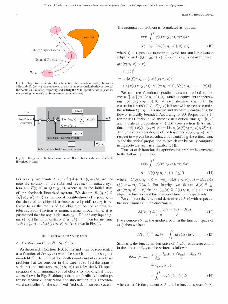
Fig. 1. Trajectories that start from the initial robust neighborhood (robustnessellipsoid)Bψ (η0 , γ) are guaranteed to stay in the robust neighborhoods aroundthe nominal (simulated) trajectory and satisfy the MTL specification φ (such asnot entering the unsafe set for a certain period of time).

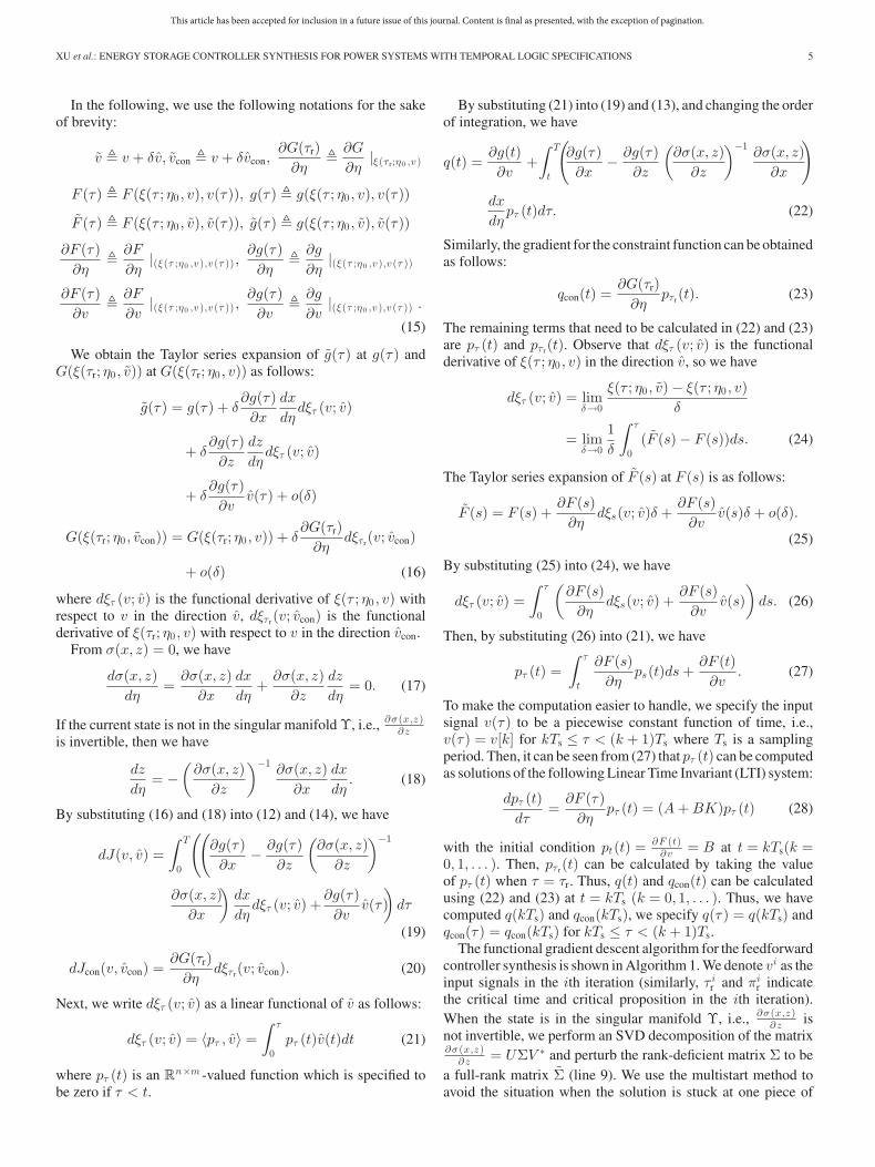
Fig. 2. Diagram of the feedforward controller with the stabilized feedbacklinearized system.

For brevity, we denote F (η, v) � (A+BK)η +Bv. We de-note the solution of the stabilized feedback linearized sys-tem η = F (η, v) as ξ(τ ; η0 , v), where η0 is the initial stateof the feedback linearized system. We denote Bψ (η, γ) �{η′|ψ(η, η′) ≤ γ} as the robust neighborhood of a point η inthe shape of an ellipsoid (robustness ellipsoid) and γ is re-ferred to as the radius of the ellipsoid. As the control au-tobisimulation function is nonincreasing through time, it isguaranteed that for any initial state η′0 ∈ Rn and any input sig-nal v(τ), if the initial distance ψ(η0 , η

′0) = γ, then for any time

τ , ξ(τ ; η′0 , v) ∈ Bψ (ξ(τ ; η0 , v), γ) (as shown in Fig. 1).

III. CONTROLLER SYNTHESIS

A. Feedforward Controller Synthesis

As discussed in Section II-B, both x and z can be representedas a function of ξ(τ ; η0 , v) when the state is not in the singularmanifold Υ. The core of the feedforward controller synthesisproblem that we consider in this paper is to find the input vsuch that the trajectory x(ξ(·; η0 , v)) satisfies the MTL spec-ification φ with minimal control efforts for the original inputu. As shown in Fig. 2, although there are feedback innerloopsfor the feedback linearization and stabilization, it is a feedfor-ward controller for the stabilized feedback linearized system.

The optimization problem is formulated as follows:

min.∫ T

0g(ξ(τ ; η0 , v), v(τ))dτ

s.t. [[φ]] (x(ξ(·; η0 , v)), 0) ≥ ζ (10)

where ζ is a positive number to avoid too small robustnessellipsoid and g(ξ(τ ; η0 , v), v(τ)) can be expressed as follows:

g(ξ(τ ; η0 , v), v(τ))

= ‖u(τ)‖2

= ||κ(x(ξ(τ ; η0 , v)), z(ξ(τ ; η0 , v)))

+ λ(x(ξ(τ ; η0 , v)), z(ξ(τ ; η0 , v))

)(Kξ(τ ; η0 , v) + v(τ))||2 .

We can use functional gradient descent method to de-crease [[¬φ]] (x(ξ(·; η0 , v)), 0), which is equivalent to increas-ing [[φ]] (x(ξ(·; η0 , v)), 0), at each iteration step until theconstraint is satisfied. AsF (η, v) is linear with respect to η and v,the solution ξ(τ ; η0 , v) is unique and absolutely continuous, theflow F is locally bounded. According to [30, Proposition 3.1],for the MTL formula ¬φ, there exists a critical time τr ∈ [0, T ]and a critical proposition πr ∈ AP (see Section II-A) suchthat [[¬φ]] (x(ξ(·; η0 , v)), 0) = Distd(x(ξ(τr; η0 , v)),O(πr)).Thus, the robustness degree of the trajectory x(ξ(·; η0 , v)) withrespect to ¬φ can be calculated by identifying the critical timeτr and the critical proposition πr (which can be easily computedusing software such as S-TaLiRo [31]).

Thus, at each iteration the optimization problem is convertedto the following problem:

min.∫ T

0g(ξ(τ ; η0 , v), v(τ))dτ

s.t. G(ξ(τr; η0 , v)) + ζ ≤ 0 (11)

where G(ξ(τr; η0 , v)) = [[¬φ]] (x(ξ(·; η0 , v)), 0) = Distd(x(ξ(τr; η0 , v)),O(πr)). For brevity, we denote J(v) �

∫ T0

g(ξ(τ ; η0 , v), v(τ))dτ and Jcon(v) � G(ξ(τr; η0 , v)) + ζ as theobjective function and the constraint function, respectively.

We compute the functional derivative of J(v) with respect tothe input signal v in the direction v,

dJ(v; v) � limδ→0

J(v + δv)− J(v)δ

. (12)

If we denote q(·) as the gradient of J in the function space ofv(·), then we have

dJ(v; v) � 〈q, v〉 =∫ T

0q(τ)v(τ)dτ. (13)

Similarly, the functional derivative of Jcon(v) with respect to vin the direction vcon can be written as follows:

dJcon(v; vcon) � limδ→0

Jcon(v + δvcon)− Jcon(v)δ

� 〈qcon, vcon〉

=∫ T

0qcon(τ)vcon(τ)dτ (14)

where qcon(·) is the gradient of Jcon in the function space of v(·).



In the following, we use the following notations for the sakeof brevity:

v � v + δv, vcon � v + δvcon,∂G(τr)∂η

� ∂G

∂η|ξ(τ r;η0 ,v )

F (τ) � F (ξ(τ ; η0 , v), v(τ)), g(τ) � g(ξ(τ ; η0 , v), v(τ))

F (τ) � F (ξ(τ ; η0 , v), v(τ)), g(τ) � g(ξ(τ ; η0 , v), v(τ))

∂F (τ)∂η

� ∂F

∂η|(ξ(τ ;η0 ,v ),v (τ )) ,

∂g(τ)∂η

� ∂g

∂η|(ξ(τ ;η0 ,v ),v (τ ))

∂F (τ)∂v

� ∂F

∂v|(ξ(τ ;η0 ,v ),v (τ )) ,

∂g(τ)∂v

� ∂g

∂v|(ξ(τ ;η0 ,v ),v (τ )) .

(15)

We obtain the Taylor series expansion of g(τ) at g(τ) andG(ξ(τr; η0 , v)) at G(ξ(τr; η0 , v)) as follows:

g(τ) = g(τ) + δ∂g(τ)∂x

dx

dηdξτ (v; v)

+ δ∂g(τ)∂z

dz

dηdξτ (v; v)

+ δ∂g(τ)∂v

v(τ) + o(δ)

G(ξ(τr; η0 , vcon)) = G(ξ(τr; η0 , v)) + δ∂G(τr)∂η

dξτ r(v; vcon)

+ o(δ) (16)

where dξτ (v; v) is the functional derivative of ξ(τ ; η0 , v) withrespect to v in the direction v, dξτ r(v; vcon) is the functionalderivative of ξ(τr; η0 , v) with respect to v in the direction vcon.

From σ(x, z) = 0, we have

dσ(x, z)dη

=∂σ(x, z)∂x

dx

dη+∂σ(x, z)∂z

dz

dη= 0. (17)

If the current state is not in the singular manifold Υ, i.e., ∂σ (x,z )∂z

is invertible, then we have

dz

dη= −

(∂σ(x, z)∂z

)−1∂σ(x, z)∂x

dx

dη. (18)

By substituting (16) and (18) into (12) and (14), we have

dJ(v, v) =∫ T

0

((∂g(τ)∂x

− ∂g(τ)∂z

(∂σ(x, z)∂z

)−1

∂σ(x, z)∂x

)dx

dηdξτ (v; v) +

∂g(τ)∂v

v(τ))dτ

(19)

dJcon(v, vcon) =∂G(τr)∂η

dξτ r(v; vcon). (20)

Next, we write dξτ (v; v) as a linear functional of v as follows:

dξτ (v; v) = 〈pτ , v〉 =∫ τ

0pτ (t)v(t)dt (21)

where pτ (t) is an Rn×m -valued function which is specified tobe zero if τ < t.

By substituting (21) into (19) and (13), and changing the orderof integration, we have

q(t) =∂g(t)∂v

+∫ T

t

(∂g(τ)∂x

− ∂g(τ)∂z

(∂σ(x, z)∂z

)−1∂σ(x, z)∂x

)

dx

dηpτ (t)dτ. (22)

Similarly, the gradient for the constraint function can be obtainedas follows:

qcon(t) =∂G(τr)∂η

pτ r(t). (23)

The remaining terms that need to be calculated in (22) and (23)are pτ (t) and pτ r(t). Observe that dξτ (v; v) is the functionalderivative of ξ(τ ; η0 , v) in the direction v, so we have

dξτ (v; v) = limδ→0

ξ(τ ; η0 , v)− ξ(τ ; η0 , v)δ

= limδ→0

1δ

∫ τ

0(F (s)− F (s))ds. (24)

The Taylor series expansion of F (s) at F (s) is as follows:

F (s) = F (s) +∂F (s)∂η

dξs(v; v)δ +∂F (s)∂v

v(s)δ + o(δ).

(25)

By substituting (25) into (24), we have

dξτ (v; v) =∫ τ

0

(∂F (s)∂η

dξs(v; v) +∂F (s)∂v

v(s))ds. (26)

Then, by substituting (26) into (21), we have

pτ (t) =∫ τ

t

∂F (s)∂η

ps(t)ds+∂F (t)∂v

. (27)

To make the computation easier to handle, we specify the inputsignal v(τ) to be a piecewise constant function of time, i.e.,v(τ) = v[k] for kTs ≤ τ < (k + 1)Ts where Ts is a samplingperiod. Then, it can be seen from (27) that pτ (t) can be computedas solutions of the following Linear Time Invariant (LTI) system:

dpτ (t)dτ

=∂F (τ)∂η

pτ (t) = (A+BK)pτ (t) (28)

with the initial condition pt(t) = ∂F (t)∂v = B at t = kTs(k =

0, 1, . . . ). Then, pτ r(t) can be calculated by taking the valueof pτ (t) when τ = τr. Thus, q(t) and qcon(t) can be calculatedusing (22) and (23) at t = kTs (k = 0, 1, . . . ). Thus, we havecomputed q(kTs) and qcon(kTs), we specify q(τ) = q(kTs) andqcon(τ) = qcon(kTs) for kTs ≤ τ < (k + 1)Ts.

The functional gradient descent algorithm for the feedforwardcontroller synthesis is shown in Algorithm 1. We denote vi as theinput signals in the ith iteration (similarly, τ ir and πir indicatethe critical time and critical proposition in the ith iteration).When the state is in the singular manifold Υ, i.e., ∂σ (x,z )

∂z isnot invertible, we perform an SVD decomposition of the matrix∂σ (x,z )∂z = UΣV ∗ and perturb the rank-deficient matrix Σ to be

a full-rank matrix Σ (line 9). We use the multistart method toavoid the situation when the solution is stuck at one piece of



Algorithm 1: Functional gradient descent algorithm.

1: Simulate the initial trajectory ξ(·; η0 , v1)

2: Run S-TaLiRo to calculate critical time τ 1r and

critical proposition π1r

3: Calculate Jcon(v1), i← 14: while

((Jcon(vi) > 0) ∨ (λ1 > ε)

) ∧ (i ≤ Nmax) do5: Calculate pτ (t) as solution of (28)6: if ∂σ (x,z )

∂z is invertible then

7: dzdη ← −

( ∂σ (x,z )∂z

)−1 ∂σ (x,z )∂x

dxdη

8: else9: Perform ∂σ (x,z )

∂z = UΣV ∗ and perturb Σ to be afull-rank matrix Σ

10: dzdη ← −(U ΣV ∗)−1 ∂σ (x,z )

∂xdxdη

11: end if12: Calculate q(t) and qcon(t) using (22) and (23)13: if Jcon(vi) ≤ 0 then14: Calculate the input signal of the next iteration

vi+1(τ)← vi(τ)− λ1q(τ)15: Simulate the trajectory of the next iteration

ξ(·; η0 , vi+1)

16: Run S-TaLiRo to calculate critical time τ i+1r ,

critical proposition πi+1r and then calculate

Jcon(vi+1)17: Calculate J(vi+1)←∑NT

k=0 g(ξ(τ [k]; η0 , vi+1),

vi+1[k])18: if J(vi+1) < J(vi) then19: λ1 ← αλ1 , α > 120: else21: λ1 ← βλ1 , 0 < β < 122: end if23: else24: Calculate the input signal of the next iteration

vi+1(τ)← vi(τ)− λ2qcon(τ)25: Simulate the trajectory of the next iteration

ξ(·; η0 , vi+1)

26: Run S-TaLiRo to calculate critical time τ i+1r ,

critical proposition πi+1r and then calculate

Jcon(vi+1)27: if Jcon(vi+1) < Jcon(vi) then28: λ2 ← αλ2 , α > 129: else30: λ2 ← βλ2 , 0 < β < 131: end if32: end if33: i← i+ 134: end while

the constraint manifold when other pieces exist. If the currentsolution satisfies the constraint, then the next solution will beoptimized along the opposite direction of the gradient of theobjective function (lines 14–22); otherwise, the next solutionwill be optimized along the opposite direction of the gradient ofthe constraint function as the constraint has to be met before theobjective function is further minimized (lines 24–31). λ1 and λ2are adjustable stepsizes. For each optimization, the algorithmterminates when the constraint is satisfied (Jcon(vi) ≤ 0) and

Fig. 3. Diagram of the feedback controller with the stabilized feedback lin-earized system.

the objective function reaches a local minimum (λ1 ≤ ε), or amaximal number of iterations is exceeded (i > Nmax ).

B. Feedback Controller Synthesis

In this section, we design a feedback control law usingsystem identification techniques to replace the optimal inputsignals of the feedforward controller. When the states andinputs of the trajectories are calculated using numeric simu-lators such as ODE or CVODE, the data are discrete and there-fore in the following we use ξ� [k] � ξ�(k; η0,� , v�) and v� [k]to denote the flow solution and the input of the �th nominal(simulated) trajectory at the kth time instant, respectively. Wedenote F �

⋃N�

�=1⋃NT , �

k=0 Bψ (ξ� [k], γ�) as the robust neighbor-hoods around the N� nominal trajectories (NT ,� is the numberof time points in the �th nominal trajectory).

Different from [23], we apply the following piecewise linearfeedback law χv (η, η′0) (as shown in Fig. 3) which depends bothon the current state η and the initial state η′0 :

χv (η, η′0) �

⎧⎪⎪⎪⎪⎨

⎪⎪⎪⎪⎩

θ1η + θ0,1 , when η ∈ X1(η′0)

θ2η + θ0,2 , when η ∈ X2(η′0)...

...

θn cη + θ0,n c , when η ∈ Xn c(η′0)

(29)

where {Xi(η′0)}n ci=1 form a partition of the state space and the

partition depends on the initial state η′0 . We use ξ(k; η′0 , χv ) todenote the flow solution of the trajectory starting from η′0 atthe kth time instant when the feedback control law χv (η, η′0)is applied. The feedback control law χv (η, η′0) and the parti-tion {Xi(η′0)}n c

i=1 have the following properties (which can beguaranteed using our design approach explained later).

Property 1: For all k > 0, � > 0, and v� that satisfies the con-straint of (10), if ξ� [k] ∈ Xj (η′0), then v� [k] = θj ξ� [k] + θ0,j −ε� [k], where ‖ε� [k]‖∞ ≤ δ, and[

P (A+BK +Bθj )P

PT (A+BK +Bθj )T P

]� 0. (30)

Property 2: If η ∈ F ∩ Xj (η′0), then there exists a ξ� [k] ∈Xj (η′0) such that η ∈ Bψ (ξ� [k], γ�).



Property 3: For any η′0 ∈⋃N�

�=1 Bψ (η0,� , γ�), if �′ =min{�|η′0 ∈ Bψ (η0,� , γ�)}, then for all k > 0, if ξ� ′ [k] ∈Xj (η′0), then ξ(k; η′0 , χv ) ∈ Xj (η′0).

Remark 1: Properties 1, 2 are modified from [23] whileProperty 3 is added in this paper as MTL specifications requiresmore stringent conditions than safety specifications in [23].

Theorem 1: If the feedback control law χv (η, η′0) and thepartition {Xi(η′0)}n c

i=1 have Properties 1, 2, and 3, then thereexists a critical radius γcrit > 0 such that if min1≤�≤N�

γ� > γcrit,the following is true for all η′0 ∈

⋃N�

�=1 Bψ (η0,� , γ�) and k > 0:�′ = min{�|η′0 ∈ Bψ (η0,� , γ�)} ⇒ ψ(ξ� ′ [k], ξ(k; η′0 , χv ))

≤ γ� ′ .Proof: Straightforward from Theorem 1, Theorem 4, and

the analysis part in the right column of [23, p. 4] while applyingProperties 1–3. �

It can be seen from Theorem 1 that if χv (η, η′0) and{Xi(η′0)}n c

i=1 have Properties 1–3 and min1≤�≤N�γ� > γcrit,

then any trajectory that starts from the initial setBψ (η0,� ′ , γ� ′) \⋃�<� ′ Bψ (η0,� , γ�) when χv (η, η′0) is applied will remain in the

robustness ellipsoids Bψ (ξ� ′ [k], γ� ′).Theorem 2: Assume that x(η) is Lipschitz continuous for

η ∈ F , i.e., ‖x(η1)− x(η2)‖ ≤ Kx‖η1 − η2‖ for any η1 ,η2 ∈ F , and some constant Kx > 0. If the feedback con-trol law χv (η, η′0) and the partition {Xi(η′0)}n c

i=1 have Prop-erties 1–3, then there exists a critical radius γcrit > 0 suchthat if min1≤�≤N�

γ� > γcrit and max1≤�≤N�γ�‖P− 1

2 ‖Kx ≤ζ(‖P− 1

2 ‖ is the largest singular value of P−12 ), then the tra-

jectory x(ξ(·; η′0 , χv )) satisfies the MTL specification φ for anyη′0 ∈

⋃N�

�=1 Bψ (η0,� , γ�).Proof: As η′0 ∈

⋃N�

�=1 Bψ (η0,� , γ�), if �′ = min{�|η′0 ∈Bψ (η0,� , γ�)}, according to Theorem 1, for all k > 0,

ψ(ξ� ′ [k], ξ(k; η′0 , χv )) = [(ξ� ′ [k]− ξ(k; η′0 , χv )

)TP(ξ� ′ [k]−

ξ(k; η′0 , χv ))]

12 ≤γ� ′ , thus ‖ξ� ′ [k]− ξ(k; η′0 , χv )‖≤γ� ′ ‖P−

12 ‖.

As for all k > 0, ξ� ′ [k] ∈ F , ξ(k; η′0 , χv ) ∈ F , so‖x(ξ� ′ [k])− x(ξ(k; η′0 , χv ))‖ ≤ Kx‖ξ� ′ [k]− ξ(k; η′0 , χv )‖ ≤Kxγ� ′ ‖P− 1

2 ‖. Therefore, if [[φ]] (x(ξ� ′ [·]), 0) ≥ ζ (from(10), here x(ξ� ′ [·]) denotes a discrete-time trajectory)and Kxγ� ′ ‖P− 1

2 ‖ ≤ max1≤�≤N�γ�‖P− 1

2 ‖Kx ≤ ζ, then[[φ]] (x(ξ� ′ [·]), 0) ≥ maxk>0 ‖x(ξ� ′ [k])− x(ξ(k; η′0 , χv ))‖,thus using the triangle inequality it can be proven that[[φ]] (x(ξ(·; η′0 , χv )), 0) ≥ 0. �

In order to satisfy Properties 1–3, in the following we describethe clustering, partitioning, and boundary modification processto determine {Xi(η′0)}n c

i=1 and χv (η, η′0).1) Clustering: The basic idea of the clustering algorithm is

to find θi and θ0,i that make the inequalities |θiξ� [k] + θ0,i −v� [k]| ≤ δ true for as many k and � as possible (maximum fea-sible subsystem problem), then remove those points and repeatthe same process over the remaining ones until all points havebeen covered (for details, see [24]). For i ≥ 2, θi and θ0,i arealso tested in the place of θj and θ0,j (j < i) in the previouscoverings. If θi and θ0,i can cover more points than θj and θ0,j ,then θj and θ0,j will be replaced by θi and θ0,i to prevent thesuboptimality of the greedy algorithm. For each candidate θi andθ0,i , we also check if (30) is satisfied to make sure that Property1 is satisfied. The clusters are further split into subclusters (byk-means or other clustering methods) until the convex hull of

Fig. 4. Piecewise linear classifiers of four sets of points with robustness el-lipsoids around them (left) and the reduced partitions with modified boundaries(right).

each subcluster is disjoint with the convex hull of any othersubcluster.

2) Partitioning: After all the disjoint subclusters are ob-tained, we classify all the subclusters using multiclass linearclassification. There are two major approaches of multiclasslinear classification: pairwise linear classifiers and piecewiselinear classifiers. The pairwise linear classifiers classify eachclass with every other class and then use the intersection of allthe half spaces determined by the pairwise decision boundariesas the partition for the class. It is easy to implement, but it isnot guaranteed to form a complete partition of the whole statespace as there may be “holes” that do not belong to any partition[24]. The piecewise linear classifier can form a complete parti-tion of the whole state space and therefore is a better fit for ourapproach. There are several different methods of constructingpiecewise linear classifiers. One way is to construct nc classifi-cation functions for thenc subclasses such that at each data pointthe corresponding class function is maximal. We use robust LPto find the nc classification functions for the nc subclasses.

Definition 3 ([32]): The nc sets Ai(i = 1, 2, . . . , nc), eachconsisting of mi

c points in Rn and represented by the n×mic

matrices Ai , are piecewise linear separable if there existsϑi, ϑj ∈ Rn , bi, bj ∈ R such that

ϑiAi − ebi > ϑjAi − ebj , i, j = 1, 2, . . . , nc, i �= j (31)

where e is a vector of ones.The classification problem becomes the following LP prob-

lem:

minϑi ,bi ,y i j

n c∑

i=1

n c∑

j=1,j �=i

eyij

mic

s.t. yij ≥ −(ϑi − ϑj )Ai + e(bi − bj ) + e

yij ≥ 0, i, j = 1, 2, . . . , nc, i �= j. (32)

3) Boundary modification: We denote the resulting parti-tion of the above LP optimization as {Xi}n c

1 . As shown inFig. 4(a), the red point does not belong to any robustness el-lipsoid within the partition X1 , but belongs to a robustnessellipsoid in another partition X2 (Property 2 is violated). Toavoid this, each partition is shrunk so that it does not intersectany robustness ellipsoid outside the partition, as shown in theshrunken partitions enclosed by the brown lines in Fig. 4(b).In the meantime, for each partition face, we make note of therobustness ellipsoids centered outside the partition and intersectthe partition face. Let Sij � {(�, k)| − ‖(ϑi − ϑj )P− 1

2 ‖γ� <



(ϑi − ϑj )ξ� [k] + bi − bj < 0} be the set of pairs (�, k) wherethe robustness ellipsoid of the �th simulated trajectory at thekth time instant (outside of Xi) intersects the decision boundarybetween the ith and jth subcluster of data. We calculate b−ij �min(�,k)∈Si j (−‖(ϑi − ϑj )P−

12 ‖γ� − (ϑi − ϑj )ξ� [k]), and thus,

obtain the new decision boundary (ϑi − ϑj )x+ b−ij = 0. Thus,

we obtain a reduced partition Xi for each original partition Xisuch that a system state within Xi is guaranteed not to belongto a robustness ellipsoid in any other partitions.

When implemented online, given the initial state η′0 , we firstcalculate �′ = min{�|η′0 ∈ Bψ (η0,� , γ�)}, then we use the fol-lowing algorithm to determine the final partition {Xi(η′0)}n c

i=1and the feedback control law χv (η, η′0).

1) If the current state η lies within the reduced partition Xi ,then η ∈ Xi(η′0), the feedback control law χv (η, η′0) =θiη + θ0,i is applied.

2) If the current state lies within the original partition Xi , butnot the reduced partition Xi , check to see if it lies withinany of the robustness ellipsoids marked in Sij (j �= i),then:

a) if it does not lie within any robustness ellipsoid cen-tered outside of Xi , then η ∈ Xi(η′0), the feedbackcontrol law χv (η, η′0) = θiη + θ0,i is applied;

b) if it lies within a unique robustness ellipsoid cen-tered at ξ� [k] and ξ� [k] lies within the jth partition(j �= i), then η ∈ Xj (η′0), the feedback control lawχv (η, η′0) = θj η + θ0,j is applied;

c) if it lies within more than one robustness ellipsoids,find the partition Xw where the state ξ� ′ [k] lies (k isthe current time instant), then η ∈ Xw (η′0), the feed-back control law χv (η, η′0) = θwη + θ0,w is applied(in this way, Property 3 is always satisfied).

IV. ENERGY STORAGE CONTROLLER SYNTHESIS

In this section, we apply the controller synthesis method indesigning an energy storage controller for regulating the gridfrequency of a double-machine infinite-bus system as shown inFig. 5 [33]. Two synchronous generators are denoted as Gi (i=1, 2), two constant power loads are denoted as L1 and L2 , andtwo constant impedance loads are denoted as L3 and L4 . TwoESSs are placed near G1 and G2 . The configuration parametersof the power system model and the line data can be seen inTables I and II. The swing dynamics of machine Gi (i = 1, 2)can be described by the following classical model:

{δi = ωiP riPb

Hi

πfsωi = Pmi − PESSi −Diωi − pei

(33)

where δi is the rotor angle position of Gi with respect to theinfinite bus at G3 , ωi is the rotor speed deviation of Gi relativeto system angular frequency 2πfs, Pb is the base power in theper unit system, Pri is the rated power of Gi , Hi is the per-unitinertia constant, Pmi is the mechanical input power to Gi , Di

is the damping coefficient, PESSi is the power that flows fromthe grid to the ESS near Gi , the electrical output power Pei

is described by the following function of δ1 , δ2 (δ3 = 0 in the

Fig. 5. Double-machine infinite-bus system.

TABLE ISYSTEM PARAMETERS

VA base Pb 160 MVASystem frequency fs 60 HzMachine rating Pri of Gi i = 1 82 MVA

i = 2 160 MVAMechanical input power Pmi i = 1 0.28 (p.u.)

i = 2 0.75 (p.u.)Active power flow to load Li i = 1 0.25 (p.u.)

i = 2 0.4375 (p.u.)i = 3 0.1875 (p.u.)i = 4 0.75 (p.u.)

Transient reactance of Gi i = 1 0.261 (p.u.)i = 2 0.284 (p.u.)

Per-unit inertia constant Hi i = 1 5 si = 2 3.5 s

Damping coefficient Di of Gi i = 1, 2 0.01 sVoltage Ei of Gi i = 1, 2 1.05 (p.u.)Transformer impedance G1 1.8868 (p.u.)

G2 0.618 (p.u.)

TABLE IILINE DATA (160 MVA BASE)

Line number Line impedance (p.u.) Line charging (p.u.)

2–8(2–9) 0.0224 + j0.1051 0.00066257–8(7–9) 0.0880 + j0.4080 0.00234–8(4–9) 0.1168 + j0.5440 0.00314–5 0.0015 + j0.0029 0.00345–6 0.0023 + j0.0032 0.00946–7 0.0053 + j0.0201 0.0258

following equation):

Pei �3∑

j=1

EiEj{Gij cos(δi − δj ) +Bij sin(δi − δj )}

+2∑

j=1

EiVj{Gij cos(δi − θj ) + Bij sin(δi − θj )}

(34)



whereEi is the voltage behind the transient reactance of Gi ,Gii

is its internal conductance,Gij + jBij is the transfer admittancebetween Gi and Gj , Gij + jBij is the transfer admittance be-tween Gi and Lj , Vj and θj are the bus voltage and bus phaseangle of Lj (j = 1, 2), respectively.

The power balance equations for the constant power loads areas follows (δ3 = 0 in the following equations):

0 = Pdi +3∑

j=1

ViEj{Gji cos(θi − δj ) + Bji sin(θi − δj )}

+2∑

j=1

ViVj{Gij cos(θi − θj ) + Bij sin(θi − θj )}

0 = Qdi +3∑

j=1

ViEj{Gji sin(θi − δj )− Bji cos(θi − δj )}

+2∑

j=1

ViVj{Gij sin(θi − θj )− Bij cos(θi − θj )} (35)

where Pdi and Qdi are the real power and reactive power ofconstant power load Li (i = 1, 2), Gji + jBji is the trans-fer admittance between Gj and Li , Gij + jBij is the transferadmittance between Li and Lj (i, j = 1, 2).

We use the following MTL specification for frequency regu-lation (here time zero represents the fault clearing time):

φ = �¬φ1 ∧�¬φ2 ∧�[2,T ]φ3 ∧�[2,T ]φ4

φ1 = (ω1 > 10), φ2 = (ω2 > 10)

φ3 = (−2 ≤ ω1 ≤ 2)∧(−2 ≤ ω2 ≤ 2)∧(−π/2 ≤ δ1 ≤ π/2)

∧ (−π/2 ≤ δ2 ≤ π/2)

which reads “The frequency deviations should never exceed 10rad/s, after 2 s the frequency deviations should always be within±2 rad/s and machine angles should always be within ±π/2.”

Assume that a three-phase lines-to-ground fault occurs nearbus 4 on lines 4–9 and the resulting fault-on system dynamicsis as follows:⎧⎪⎪⎪⎪⎪⎪⎪⎨

⎪⎪⎪⎪⎪⎪⎪⎩

x1 = x3

x2 = x4

x3 = 74.3059(0.28− 0.01x3 − (0.0027808− 0.00045389

· cos(x1) + 0.054597 sin(x1)− 0.0020063z3

· cos(x1 − z1) + 0.30751z3 sin(x1 − z1)))

x4 = 53.8559(0.75− 0.01x4

)⎧⎪⎪⎪⎪⎪⎪⎪⎪⎪⎪⎪⎨

⎪⎪⎪⎪⎪⎪⎪⎪⎪⎪⎪⎩

0 = −0.25− (0.0020063z3 cos(z1 − x1) + 0.30751z3

· sin(z1 − x1)− 0.76927z3 cos(z1) + 3.5329z3 sin(z1)+1.3459z2

3 )0 = −0.4375− (−12.1574z4 cos(z2) + 46.4191z4 sin(z2)

+84.8243z24 )

0 = 0.0020063z3 sin(z1 − x1)− 0.30751z3 cos(z1 − x1)−0.76927z3 sin(z1)− 3.5329z3 cos(z1) + 6.4861z2

3

0 = −12.157z4 sin(z2)− 46.419z4 cos(z2) + 164.647z24

where the state x = [δ1 , δ2 , ω1 , ω2 ]T , z = [θ1 , θ2 , V1 , V2 ]T .

Fig. 6. Simulated postfault trajectories with no storage input with fault clear-ing time of 0.19 and 0.2 s.

After the fault is cleared, the postfault system with the inputu = [PESS1 , PESS2 ]T is as follows:⎧⎪⎪⎪⎪⎪⎪⎪⎪⎪⎪⎪⎪⎨

⎪⎪⎪⎪⎪⎪⎪⎪⎪⎪⎪⎪⎩

x1 = x3

x2 = x4

x3 = 74.3059(0.28− u1 − 0.01x3 − (0.003− 0.00062

· cos(x1) + 0.0683 sin(x1)− 0.00237z3 cos(x1 − z1)+0.3336z3 sin(x1 − z1))

)

x4 = 53.8559(0.75− u2 − 0.01x4 − (0.00447 + 0.00455z3

· cos(x2 − z1) + 0.0134z3 sin(x2 − z1)− 0.0083z4

· cos(x2 − z2) + 1.0875z4 sin(x2 − z2)))

⎧⎪⎪⎪⎪⎪⎪⎪⎪⎪⎪⎪⎪⎪⎪⎪⎪⎪⎪⎪⎪⎪⎪⎪⎪⎪⎪⎪⎨

⎪⎪⎪⎪⎪⎪⎪⎪⎪⎪⎪⎪⎪⎪⎪⎪⎪⎪⎪⎪⎪⎪⎪⎪⎪⎪⎪⎩

0 = −0.25− (−0.0023695z3 cos(z1 − x1) + 0.3336z3

· sin(z1 − x1) + 0.00455z3 cos(z1 − x2) + 0.013353z3

· sin(z1 − x2)− 0.84z3 cos(z1) + 3.83z3 sin(z1) + 1.47−0.38326z3z4 cos(z1 − z2) + 1.7208z3z4 sin(z1 − z2))

0 = −0.4375− (−0.008316z4 cos(z2 − x2) + 1.0875z4

· sin(z2 − x2)− 12.1574z4 cos(z2) + 46.4191z4 sin(z2)−0.38326z3z4 cos(z2 − z1) + 1.7208z3z4 sin(z2 − z1)+13.1715z2

4 )0 = −0.0023695z3 sin(z1 − x1)− 0.3336z3 cos(z1 − x1)

+0.0045526z3 sin(z1 − x2)− 0.013353z3 cos(z1 − x2)−0.83677z3 sin(z1)− 3.8322z3 cos(z1) + 5.8948z2

3

−0.38326z3z4 sin(z1 − z2)− 1.7208z3z4 cos(z1 − z2)0 = −0.008316z4 sin(z2 − x2)− 1.0875z4 cos(z2 − x2)−12.1574z4 sin(z2)− 46.4191z4 cos(z2)− 0.3833z3z4

· sin(z2 − z1)− 1.7208z3z4 cos(z2 − z1) + 49.1724z24 .

We assume that the fault is cleared between 0.19 and 0.2 s. Asshown in Fig. 6, the postfault system with no storage input (u1 =u2 = 0) is not stable as the two generators lose synchronismsoon after the fault is cleared. Therefore, an energy storagecontroller is necessary not only for the purpose of frequencyregulation, but also for maintaining the transient stability of thepostfault system.

We first feedback linearize the postfault system using theM derivative. By choosing the output functions as h1(x, z) =x1 , h2(x, z) = x2 , the postfault feedback linearized system isas follows:

⎧⎪⎨

⎪⎩

η1 = η2η2 = ρ1η3 = η4η4 = ρ2



where the new state η = [x1 , x3 , x2 , x4 ]T , ρ = [ρ1 , ρ2 ]T is theinput of the feedback linearized system. κ(x, z) and λ(x, z) in(4) are calculated as follows:

λ(x, z) =

[− 1

74.3059 0

0 − 153.8559

]

κ(x, z) =

⎡

⎢⎢⎢⎢⎢⎢⎢⎢⎣

0.28− 0.01x3 − (0.003− 0.00062 cos(x1)

+0.0683 sin(x1)− 0.00237z3 cos(x1 − z1)

+0.3336z3 sin(x1 − z1));

0.75− 0.01x4 − (0.00447 + 0.00455z3

· cos(x2 − z1) + 0.0134z3 sin(x2 − z1)− 0.0083

·z4 cos(x2 − z2) + 1.0875z4 sin(x2 − z2))

⎤

⎥⎥⎥⎥⎥⎥⎥⎥⎦

.

We then introduce input v and let ρ(η) = Kη + v, where

K =[−0.8068 −0.9894 0 0

0 0 −0.8068 −0.9894

]

is calculated using (9). The obtained system η = F (η, v) =(A+BK)η +Bv is a stabilized linear system with the newinput v.

To optimize v for the feedforward controller synthesis, weuse Algorithm 1 and set T = 10 s, Ts = 0.1 s, ζ = 0.3,Nmax =100, ε = 10−6 , λ1 = λ2 = 1 (initial values), α = 1.5, β = 0.2(all the values are per unit values unless otherwise specified). Wesimulate three trajectories of the postfault feedback linearizedsystem starting from the fault-on trajectories cleared at 0.1912 s,0.195 s, and 0.1995 s respectively. The optimal input signal vand the corresponding storage input u for the three differentfault clearing time are shown in Fig. 7. It can be seen that inall three different scenarios, the power flows from the grid tothe ESSs near G1 and G2 significantly in the first 1 to 2 s todecrease the grid frequency. After this period, the power flowchanges direction as the frequency deviation becomes negativeand continues to decrease, so the ESSs have to inject powerto the grid to prevent the frequency from dropping beyond thelower threshold. After the first 5 s, the storage control effortsgradually decrease to zero. It can also be seen that with longerfault clearing time, more (storage) control effort is needed tosatisfy the MTL specification φ.

The initial robustness ellipsoid of the simulated postfault tra-jectory with fault clearing time of 0.195 s totally covers thesimulated fault-on trajectory from 0.19 to 0.2 s (the postfaultinitial states), as shown in Fig. 8. Thus, all the possible post-fault trajectories with the given uncertainties in the fault clearingtime (between 0.19 and 0.2 s) are guaranteed to satisfy the MTLspecification φ (as shown in Fig. 9).

Next, we design a piecewise linear feedback law that islearned from the data of the simulated trajectory and the corre-sponding optimal inputs. We first cluster the 1001 data pointsinto 94 disjoint subclusters while in each subcluster the input er-ror is within δ = 0.0118 (as γcrit depend on δ [23], δ is designedsuch that min1≤�≤N�

γ� > γcrit and max1≤�≤N�γ�‖P− 1

2 ‖Kx ≤ζ, here N� = Kx = 1), as shown in Fig. 10. We generatethe piecewise linear classifier to separate the 94 subclus-ters and modify the partitions using the method described inSection III-B. We generate 20 postfault trajectories with the

Fig. 7. New input v and storage input u (blue for ESS 1 and green for ESS 2)of the feedforward controller with fault clearing time of: (a), (b) 0.1912 s, (c),(d) 0.195 s, (e), (f) 0.1995 s.

Fig. 8. Coverage of the simulated fault-on trajectory from 0.19 to 0.2 s (red)with the initial robustness ellipsoid (black) of the simulated postfault trajectorywith fault clearing time of 0.195 s.

Fig. 9. Robust neighborhoods (red) of the nominal (simulated) postfault tra-jectory (black) with fault clearing time of 0.195 s.



Fig. 10. Subclusters obtained from the bounded-error clustering approach(different colors represent different subclusters).

Fig. 11. Twenty postfault trajectories generated with the feedback controllerover a sampling of initial conditions (fault clearing time between 0.19 and 0.2 s).

Fig. 12. Twenty postfault trajectories generated with the feedforward con-troller (a) and the feedback controller, (b) over a sampling of initial conditions(fault clearing time between 0.19 and 0.2 s) with the disturbance of value−20 in the first dimension of the input v during the first 0.2 s.

feedback controller over a sampling of initial conditions andthe trajectories all satisfy the MTL specification φ (as shown inFig. 11).

To make a comparison between the feedback controller andthe feedforward controller, we add a disturbance of value−20 tothe first dimension of the input v during the first 0.2 s while gen-erating the 20 postfault trajectories with both the feedforwardand the feedback controllers over a sampling of initial condi-tions (fault clearing time between 0.19 and 0.2 s). As shown inFig. 12(a), with the feedforward controller, although the rotorspeed deviation ω1 still gradually approaches zero, ω1 crosses−2 rad/s in the process as the inputs are precomputed and thusunresponsive to the unexpected disturbance. In comparison, asshown in Fig. 12(b), with the feedback controller, the rotorspeed deviation ω1 is always greater than −2 rad/s as the feed-back controller adjusts the inputs according to the feedback law,

thus the states remain in the robust neighborhoodsF despite theunexpected disturbances.

V. CONCLUSION

We presented a controller synthesis framework to control theESSs with MTL specifications. We model the power system asa nonlinear DAE system and both the feedforward and the feed-back controller synthesis for such DAE systems are presented.The controller synthesis approach can be used in other relatedareas in power systems such as transient stability enhancement,voltage regulation, etc. Similar approaches can be also appliedto other nonlinear DAE systems such as robotic systems, bio-logical systems, etc.

ACKNOWLEDGMENT

The authors would like to thank Dr. A. K. Winn for helpfuldiscussions.

REFERENCES

[1] F. Delfino, F. Pampararo, R. Procopio, and M. Rossi, “A feedback lin-earization control scheme for the integration of wind energy conversionsystems into distribution grids,” IEEE Syst. J., vol. 6, no. 1, pp. 85–93,Mar. 2012.

[2] Z. Xu, A. A. Julius, and J. H. Chow, “Robust testing of cascading failuremitigations based on power dispatch and quick-start storage,” IEEE Syst.J., to be published.

[3] A. D. Papalexopoulos and P. E. Andrianesis, “Performance-based pricingof frequency regulation in electricity markets,” IEEE Trans. Power Syst.,vol. 29, no. 1, pp. 441–449, Jan. 2014.

[4] A. Mondal, S. Misra, and M. S. Obaidat, “Distributed home energy man-agement system with storage in smart grid using game theory,” IEEE Syst.J., vol. 11, no. 3, pp. 1857–1866, Sep. 2017.

[5] S. W. Mohod and M. V. Aware, “Micro wind power generator with batteryenergy storage for critical load,” IEEE Syst. J., vol. 6, no. 1, pp. 118–125,Mar. 2012.

[6] A. K. Srivastava, A. A. Kumar, and N. N. Schulz, “Impact of distributedgenerations with energy storage devices on the electric grid,” IEEE Syst.J., vol. 6, no. 1, pp. 110–117, Mar. 2012.

[7] Z. Xu, C. Belta, and A. A. Julius, “Temporal logic inference with prior in-formation: An application to robot arm movements,” IFAC-PapersOnLine,vol. 48, no. 27, pp. 141–146, 2015.

[8] Z. Xu, M. Birtwistle, C. Belta, and A. Julius, “A temporal logic inferenceapproach for model discrimination,” IEEE Life Sci. Lett., vol. 2, no. 3,pp. 19–22, Sep. 2016.

[9] P. Tabuada, Verification and Control of Hybrid Systems: A SymbolicApproach. New York, NY, USA: Springer, 2009. [Online]. Available:https://books.google.com/books?id=1ExhrqtzIYwC

[10] E. M. Wolff, U. Topcu, and R. M. Murray, “Automaton-guided controllersynthesis for nonlinear systems with temporal logic,” in Proc. IEEE/RSJInt. Conf. Intell. Robots Syst., Nov. 2013, pp. 4332–4339.

[11] S. Coogan, E. A. Gol, M. Arcak, and C. Belta, “Traffic network controlfrom temporal logic specifications,” IEEE Trans. Control Netw. Syst.,vol. 3, no. 2, pp. 162–172, Jun. 2016.

[12] A. Donze and V. Raman, “Blustl: Controller synthesis from signal tempo-ral logic specifications,” in ARCH@CPSWeek, 2015.

[13] S. Saha and A. A. Julius, “An MILP approach for real-time optimalcontroller synthesis with metric temporal logic specifications,” in Proc.IEEE Amer. Control Conf., Jul. 2016, pp. 1105–1110.

[14] A. K. Winn and A. A. Julius, “Optimization of human generated trajec-tories for safety controller synthesis,” in Proc. IEEE Amer. Control Conf.,Jun. 2013, pp. 4374–4379.

[15] H. Abbas, A. Winn, G. Fainekos, and A. A. Julius, “Functional gradientdescent method for metric temporal logic specifications,” in Proc. IEEEAmer. Control Conf., Jun. 2014, pp. 2312–2317.

[16] S. Sastry and C. Desoer, “Jump behavior of circuits and systems,” IEEETrans. Circuits Syst., vol. 28, no. 12, pp. 1109–1124, Dec. 1981.

[17] D. Karimipour and F. R. Salmasi, “Stability analysis of ac microgridswith constant power loads based on popov’s absolute stability criterion,”IEEE Trans. Circuits Syst. II, Express Briefs, vol. 62, no. 7, pp. 696–700,Jul. 2015.



[18] X. Lu, K. Sun, J. M. Guerrero, J. C. Vasquez, L. Huang, and J. Wang,“Stability enhancement based on virtual impedance for dc microgrids withconstant power loads,” IEEE Trans. Smart Grid, vol. 6, no. 6, pp. 2770–2783, Nov. 2015.

[19] Y. Li and J. Liu, “Switching control of differential-algebraic equationswith temporal logic specifications,” in Proc. IEEE Amer. Control Conf.,Jul. 2015, pp. 1941–1946.

[20] M. Althoff and B. H. Krogh, “Reachability analysis of nonlineardifferential-algebraic systems,” IEEE Trans. Automat. Control, vol. 59,no. 2, pp. 371–383, Feb. 2014.

[21] Z. Xu, A. A. Julius, and J. H. Chow, “Optimal energy storage control forfrequency regulation under temporal logic specifications,” in Proc. Amer.Control Conf., Seattle, WA, USA, May 2017, pp. 1874–1879.

[22] A. A. Julius, “Trajectory-based controller design for hybrid systems withaffine continuous dynamics,” in Proc. IEEE Int. Conf. Autom. Sci. Eng.,Aug. 2010, pp. 1007–1012.

[23] A. K. Winn and A. A. Julius, “Feedback control law generation for safetycontroller synthesis,” in Proc. IEEE Conf. Decision Control, Dec. 2013,pp. 3912–3917.

[24] A. Bemporad, A. Garulli, S. Paoletti, and A. Vicino, “A bounded-errorapproach to piecewise affine system identification,” IEEE Trans. Autom.Control, vol. 50, no. 10, pp. 1567–1580, Oct. 2005.

[25] G. E. Fainekos and G. J. Pappas, “Robustness of temporal logic specifi-cations for continuous-time signals,” Theoretical Comput. Sci., vol. 410,no. 42, pp. 4262–4291, 2009.

[26] G. E. Fainekos and G. J. Pappas, “Robustness of temporal logic specifica-tions,” in Proc. 1st Combined Int. Conf. Formal Approaches Softw. TestingRuntime Verification, 2006, pp. 178–192.

[27] J. Wang and C. Chen, “Exact linearization of nonlinear differential al-gebraic systems,” in Proc. Int. Conf. Info-Tech Info-Net, 2001, vol. 4,pp. 284–290.

[28] A. R. Khudair, “State linearization of multi-input nonlinear differentialalgebraic control systems,” Int. J. Contemp. Math. Sci., vol. 8, no. 11,pp. 499–509, 2013.

[29] S. Kolavennu, S. Palanki, and J. Cockburn, “Nonlinear controlof nonsquare multivariable systems,” Chemical Eng. Sci., vol. 56,no. 6, pp. 2103–2110, 2001. [Online]. Available: http://www.sciencedirect.com/science/article/pii/S000925090000470X

[30] H. Abbas and G. Fainekos, “Computing descent direction of MTL ro-bustness for non-linear systems,” in Proc. IEEE Amer. Control Conf.,Jun. 2013, pp. 4405–4410.

[31] Y. Annpureddy, C. Liu, G. Fainekos, and S. Sankaranarayanan, S-TaLiRo:A Tool for Temporal Logic Falsification for Hybrid Systems. Berlin,Germany: Springer, 2011, pp. 254–257.

[32] K. P. Bennett and O. L. Mangasarian, “Multicategory discrimination vialinear programming,” Optimization Methods Softw., vol. 3, pp. 27–39,1992.

[33] Y. Susuki, T. Sakiyama, T. Ochi, T. Uemura, and T. Hikihara, “Verifyingfault release control of power system via hybrid system reachability,” inProc. 40th North Amer. Power Symp., Sep. 2008, pp. 1–6.

Zhe Xu (S’16) received the B.S. and M.S. degreesin electrical engineering from Tianjin University,Tianjin, China, in 2011 and 2014, respectively. Heis currently working toward the Ph.D. degree in elec-trical engineering at the Rensselaer Polytechnic In-stitute, Troy, NY, USA.

His research interests include temporal logic, sys-tems and control, hybrid systems, and power systems.

Agung Julius (M’06) received the Ph.D. degree inapplied mathematics from the University of Twente,Enschede, The Netherlands, in 2005.

From 2005 to 2008, he was a PostdoctoralResearcher with the University of Pennsylvania,Philadelphia, PA, USA. Since 2008, he has been withthe Department of Electrical, Computer, and SystemsEngineering, Rensselaer Polytechnic Institute, Troy,NY, USA, where he is currently an Associate Profes-sor. His research interests include systems and con-trol, systems biology, stochastic models in systems

biology, control of biological systems, hybrid systems, and mathematical sys-tems theory.

Joe H. Chow (F’92) received the B.S. degree fromthe University of Minnesota, Minneapolis, MN, USA,and the M.S. and Ph.D. degrees from the Universityof Illinois, Urbana–Champaign, IL, USA.

After working with General Electric Power Sys-tem Business, Schenectady, NY, USA, he joined theRensselaer Polytechnic Institute in 1987, and is aProfessor of electrical, computer, and systems engi-neering and the Campus Director of the NSF/DOECURENT ERC. His research interests include powersystem dynamics and control, renewable resources,

voltage stability, and synchronized phasor data.Dr. Chow was the recipient of the Donald Eckman Award of American Au-

tomatic Control Council, the Control System Technology Award of the IEEEControl System Society, and the Charles Concordia Power System EngineeringAward of the IEEE Power and Energy Society. He is a member of the NationalAcademy of Engineering.

Documents

IEEE SYSTEMS JOURNAL 1 Energy Storage Controller Synthesis