Embed Size (px)
DESCRIPTION
PREDICTION METHOD FOR BURIED PIPELINE VOLTAGESDUE TO 60 Hz AC INDUCTIVE COUPLING
Citation preview
780 IEEE Transactions on Power Apparatus and Systems, Vol. PAS-98, No. 3 May/June 1979
PREDICTION METHOD FOR BURIED PIPELINE VOLTAGESDUE TO 60 Hz AC INDUCTIVE COUPLING
PART I - ANALYSIS
Allen Taflove, Member, IEEE John Dabkowski, Non-MemberIIT Research Institute10 West 35th Street
Chicago, Illinois 60616
Abstract - The voltages induced on gas transmis-sion pipelines by 60 Hz ac power transmission linessharing a joint right-of-way are predicted using elec-trical transmission line theory. Thevenin equivalentcircuits for pipeline sections are developed whichallow the decomposition of complex pipeline-power linegeometries. Programmable hand calculator techniquesare used to determine inducing fields, pipeline char-acteristics, and Thevenin circuits.
INTRODUCTION
Since January 1976, IIT Research Institute hasbeen funded jointly by the Electric Power ResearchInstitute and the American Gas Association to consoli-date known data concerning the effects of voltagesinduced on gas transmission pipelines by6OHz ac powertransmission lines sharing a joint right-of-way. Thegoal of the study is the writing of a tutorial hand-book that can be used by field personnel topredicttheinduced pipeline voltages and institute measures tomitigate against accompanying effects.
This paper presents the prediction method devel-oped by IITRI for the induced voltages on buried pipelines. The approach utilizes electrical transmissionline theory to locate and quantize pipeline voltagepeaks using a programmable hand calculator. Complexac power line features such as multiple circuits,shield wires, and phase transpositions can be modeledin a systematic way. The approach developed has provento be more accurate than existing methods in fieldtests, and i s appl i cabl e to real i sti c pi pel i ne-ac powerline corridors. The methodology and results of thesefield tests are discussed in Part II of this paper.
This paper first reviews available analyticalmethods for the prediction of inductive coupling toburied pipelines. Next, the basic elements of the newapproach are presented. Equations and equivalent cir-cuits are derived to estimate inductive coupling forthe following cases of pipeline construction near anac power transmission line:
1) parallel construction;2) non-parallel construction;3) combinations of parallel and non-parallel
constructions and power line discontinuities.
The required numerical inputs to the equations andequivalent circuits are obtained using hand calculatorprograms developed by IITRI. The capabi l i ti es of these
F 78 698-3. A paper recacuended and approved bythe ]flI Insulated Ccnductors Camiittee of the IEEEPcwer Engineering Society for presentatio at theIEEE PES Suimr Meeting, Los Angeles, CA, July 16-21, 1978. Manuscript submitted February 1, 1978;made available for printing May 3, 1978.
tools are briefly summarized in the last section ofthis paper.
REVIEW OF AVAILABLE ANALYTICAL TECHNIQUES
For many years, concern was directed to couplingbetween overhead high voltage ac power lines and adja-cent above-ground communication circuits. Equationspresented originally by Westinghouse1 have been usedto predict the induced voltage per mile on an above-ground conductor due to single phase and three phaseac power lines. An equivalent approach2 used Carson'sseries3 to compute the mutual impedances between thepower line conductors and the affected communicationsline. The International Telegraph and Telephone Con-sultative Committee (CCITT) has summarized availableprediction and mitigation methods for induced voltageson above-ground conductors.4
One body of literature has attempted to apply theabove-ground coupling equations directly tohthcase ofthe buried pipeline. Representative papers deter-mined the induced pipeline voltage in the followinggeneral way:
Vmax = f(I,d)-L (1)
where Vmax is the maximum expected voltage; f is somefunction of power line current, I, and distance, d,from the pipeline; and L isthe length of the pipeline.Uniformly, the values of pipeline voltage calculatedusing these methods are too high by a factor gff bout10, as acknowledged by several of the workers. ,1
The application of the above-ground equations failsfor the buried pipeline case simply because a buriedpi pel i ne di ffers el ectri cal ly from an overhead conductor.A buried pipeline, either bare or wrapped in an elec-trically insulating coating, hasa finite resistance toearth distributed over its entire length, whereas anoverhead line has, at most, point grounds at largeintervals. To describe the distributed interactionbetween a buried pipeline and its surrounding earth,factors such as pi pel i ne di ameter, coati ng conducti vi ty,earth resistivity, depth of burial , and pipe longitudi-nal resistance and inductance must be taken into account.
A second body of literature has attempted to con-struct such a realistic model of inductive coupling toa buried pipeline. The analytical approach used inthese references considers a buried pipeline as a lossyelectrical transmission line with a distributed voltagesource function due to electromagnetic couplii. How-ever, available published work in this area hasevidently failed to achieve accurate methods simplifiedenough for widespread usage by the pipeline and powerline communities.
THE DISTRIBUTED SOURCE ANALYSIS APPROACH
The analysis of this paper treats inductive cou-pling to arbitrary buried pipelines using, a theorycalled the distributed source analysis.15"l6 Here, apipeline and its surrounding earth form a lossy elec-trical transmission line characterized by the propagation
0018-9510/79/0500-780$00.75 © 1979 IEEE
constant,y, and the characteristic impedance? Z Theinductive coupling effect of a nearby ac power 7ine isincluded by defininga distributed voltage source func-tion, Ex(s), along the pipeline, where Ex(s) is thelongitudinal driving electric field parallel to thepath of the pipeline.
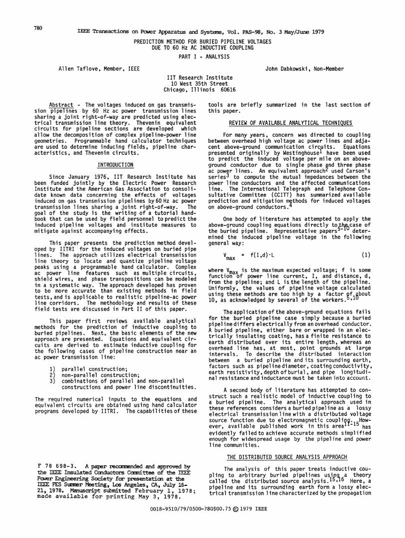
As shown in Fig. 1, specific couplingproblemsaretreated as special cases of the general distributedsource theory. The general theory is first special-ized with respect to the orientation of the pipelinesection relative to the adjacent ac power line:
1) parallel case (pipeline section parallelto the ac power line);
2) non-parallel case (pipeline section at anangle to the ac power line).
General Theory for Single-Section Pipelines
1. Parallel Case 2. Non-Parallel Case
a. Short b. Long/ a. Short b. Long/Lossy Lossy
Thevenin Thevenin Thevenin TheveninEquivalent Equivalent Equivalent EquivalentCircuit Circuit Circuit Circuit
Node Analysis of Arbitrary Pipeline/Powerl ine Co-Locations
Fig. 1. Application of the Distributed Source Analysis
The theory is further specialized by grouping pipelinesections according to electrical length:
la, 2a) Electrically short case
L < 0.1 300OmFT7where L is the length of the pipelinesection
lb, 2b) Electrically long-lossy case
L > 2 -10 km.Real (y) -
As shown later in this paper, the terminal beha-vior of pipeline sections of Classes la, lb, 2a, and2b can be described by simple Thevenin equivalent cir-cuits. These circuits can be connected together toallow predictionof the inductive coupling to pipelinesof arbitrary geometry and composedof several connecteddissimilar sections
General Analysis
In this analysis, each pipeline length increment,
781
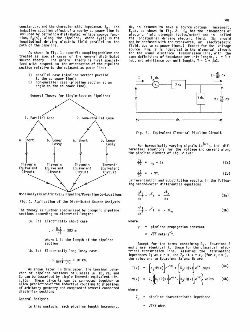
dx, is assumed to have a source voltage increment,Exdx, as shown in Fig. 2. Ex has the dimensions ofelectric field strength (volts/meter) and is calledthe longitudinal driving electric field. (Ex shouldnot be confused with the transverse, or electrostaticfield, due to ac power lines.) Except for the voltagesource, Fig. 2 is identical to the elemental circuitfor the usual electrical transmission line, with thesame definitions of impedance per unit length, Z - R +jwL, and admittance per unit length, Y = G + jwC.
I+ d4 dxdx
dx
dx
Fig. 2. Equivalent Elemental Pipeline Circuit
For harmonically varying signals (eiwt), the dif-ferential equations for the voltage and current alongthe pipeline element of Fig. 2 are:
dV - E - IZdx- x
dI - VY.
(2a)
(2b)Differentiation and substitution results in the follow-ing second-order differential equations:
d2V 2V- YdxJdExx
dx(3a)
(3b)d2 2I = -YEdx x
where
y = pipeline propagation constant
= Y meters
Except for the terms containing E, Equations 2and 3 are identical to those for the cfassical elec-trical transmission line. Assuming the terminatingimpedances Z1 at x = xi and Z2 at x = x2 (for x2>x1),the solutions to Equations 3a and 3b are
I(x) = [K1+P(x)}eYx + [K2+Q(x)]eYx amps (4a)
V( = Zo Kl+P(x)eY-xK2+Q(x)1eYx} volts (4b)
where
ZO= pipeline characteristic impedance
=vZ/Y ohms
782
x
P(x) = 41 - eys E (s) ds
.x 1
X2Q(x) = 2ZIf eTys E (s) ds
xZ
yx= P -P(xx)eY2-Q(x)e x2K1 = Pie eY(X2 2)p p2e Y(X2X
Yx1 -Yxl-yx2 P1Q(x1)e -P(x2 )e
K2 p2e --eK(x2-2x=e1 P1p2e-Y(X2-x1)
and P1,P2 are reflection coefficients given by:
Substituting Ex(s) = Eo into Equations 5a and 5b(5a) results in
(5b)
(6a)
x
Q(x) = C e-ys
Usingyields:
E L"
Ends = 2 (eX- e1) .
o 2yZ0
(8a)
(8b)
the results of Equation 8 in Equation 6
P= E P2 (1-e yL ) + 1-eyL
K1 2yZ0 eyL _ pe rL J(6b)(9a)
(9b)P2E2ey2 [Pi ( l-eYL)+ 1-eyLK2 - 2yZ- LyeL P12y~L
P1= ,i-ZOz1+zoZ2-Zo
p2 - Z2+z0 (7) Substituting K1, K2, P(x), and Q(x) into Equation 4b,the general so ution for V(x) in terms of the termina-ting impedances, Z1 and Z2' is obtained:
Using Equations 4-7, the analysis presented per-mits general treatmentof inductive coupling to a buriedpipeline having an arbitrary, but constant, y and ZO;arbitrary terminations Z1 and Z2; and arbitrary drivingfield Ex(s). The analyses to follow will treat specialcases of the general analysis. In doing so, certainspecial characteristics of inductive coupling to bur-ied pipelines will become apparent. Further, the treat-ment of pipes having discontinuities of either y, Zo,or Ex(s) will be discussed. Methods for computing y,ZO, and Ex(s) are deferred to the end of this paper.
Application to the Parallel PipelineWith Arbitrary Terminations
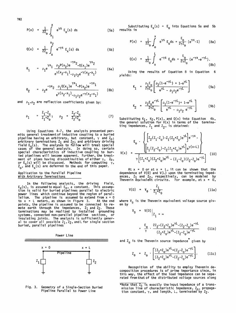
In the following analysis, the driving field,Ex(s), is assumedto equal Eo, a constant. This assump-tion is valid for buried pipelines parallel to electricpower lines which continue beyond the region of paral-lelism. The pipeline is assumed to extend from x = 0to x = L meters, as shown in Figure 3. At the endpoints, the pipeline is assumed to be connected to re-mote earth through the impedances, Zl and Z2. Theseterminations may be realized by installed groundingsystems, connected non-parallel pipeline sections, orinsulating joints. The analysis is sufficiently gener-al to cover all possible Z1,Z2,andLfor single sectionburied, parallel pipelines
Power Line
x = 0 x = L
z1
[Z2(-z )-Z (Z2+Z )eyJeYx_
tt l(Z2- z0)- 2(Zi+Z0)eyL]ey(x-L)V(x) = (10)
Y[(Z1+Zo) (Z2+Z0)eyL - (Z1-z0) (Z2-Z0)eyLJ
At x = O or at x = L, it can be shown that thedependence of V(O) and V(L) upon the terminating imped-ances, Z1 and Z2, respectively, can be modeled byThevenin equivalent circuits. For example, at x = 0,
V1v(o) = V0 (ha)+whereVb is the Thevenin equivalent voltage source giv-en by
V - V(O)Z1 =
_ E0 2Z2-(Z2+ZO)eyL(Z2-Z )e yLr (Z2+Z )eYL_ (Z2 Z )eYL
and Z0 is the Thevenin source impedance given by
[Zo z+z. )eyL_(ZZ__ )e_ Y]
(llb)
(lic)
Z2
Fig. 3. Geometry of a Single-Section BuriedPipeline Parallel to Power Line
Recognition of the ability to employ Thevenin de-composition procedures is of prime importance since, inthis way, the effect of the load impedance can be sepa-rated fromthatof the distributed voltage sources along
*Note that Z0 is exactly the input impedance of a trans-mission line of characteristic impedance, ZO, propaga-tion constant, y, and length, L, terminated by Z2.
(lla)
the pipe. Thus, the analysis of a multi-section pipe-line or a pipeline subject to sharp variations of in-ducing field because of geometrical or electrical dis-continuities can be treated by applying Thevenin pro-cedures at the junctions or field discontinuities, asdiscussed later in this paper.
Equations 10 and 11 will now be simplifiedforthetwo most important pipeline cases: the electricallyshort pipeline; and the electrically long/lossy pipe-line.
The Electrically Short Pipeline For this analysis,the length, L, of an electricallyshortpipeline satis-fies the inequality
L < 01 -300m1Y7K
783
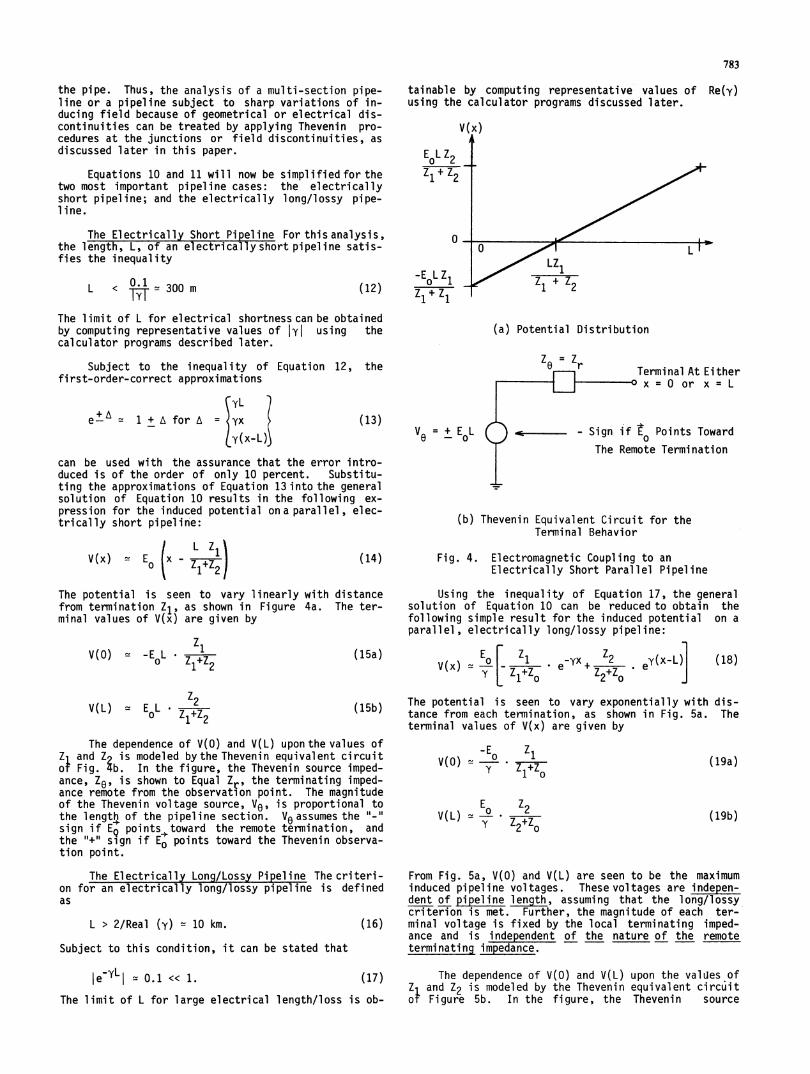
tainable by computing representative values of Re(y)using the calculator programs discussed later.
V(x)4
EoL Z2Z1 + Z2
O
-E( LZ(12) ol+z1+1
0LZ1
z1 + Z2
LI
The l imi t of L for el ectri cal shortness can be obtai nedby computing representative values of hyI using thecalculator programs described later.
Subject to the inequality of Equation 12, thefirst-order-correct approximations
(a) Potential Distribution
Terminal At Eitherx = 0 or x = L
e+A - 1 + A for A = yx
y(x-L)}(13)
can be used with the assurance that the error intro-duced is of the order of only 10 percent. Substitu-ting the approximations of Equation 13 into the generalsolution of Equation 10 results in the following ex-pression for the induced potential ona parallel, elec-trically short pipeline:
V(x) = E (x - z +__ (14)
The potential is seen to vary linearly with distancefrom termination Z1, as shown in Figure 4a. The ter-minal values of V(x) are given by
z1V(O) = -E0L Z +Z (15a)
z2V(L) E0L * Z +Z (15b)
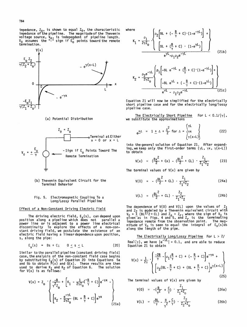
The dependence of V(O) and V(L) uponthevalues ofZ1 and Z& is modeled bytheThevenin equivalent circuitof Fig. 4b. In the figure, the Thevenin source imped-ance, Z0, is shown to Equal Zr, the terminating imped-ance remote from the observation point. The magnitudeof the Thevenin voltage source, Ve, is proportional tothe length of the pipeline section. Ve assumes thesign if EQ points-toward the remote termination, andthe "+" sign if Eo points toward the Thevenin observa-tion point.
The Electrically Long/Lossy Pipeline The criteri-on for an electrically long/lossy pipeline is definedas
L > 2/Real (y) 10 km. (16)
Subject to this condition, it can be stated that
leyL = 0.1 << 1. (17)The limit of L for large electrical length/loss is ob-
Ve =+ EoL Sign if t Points Toward0
The Remote Termination
(b) Thevenin Equivalent Circuit for theTerminal Behavior
Fig. 4. Electromagnetic Coupling to anElectrically Short Parallel Pipeline
Using the inequality of Equation 17, the generalsolution of Equation 10 can be reduced to obtain thefollowing simple result for the induced potential on aparallel, electrically long/lossy pipeline:
E0[*e1 yx+ Z2 y(x-L)l
V(x) e(18)
The potential is seen to vary exponentially with dis-tance from each termination, as shown in Fig. 5a. Theterminal values of V(x) are given by
-E0V(O) = ° . +ZV(0L) y * Z2
E0
zV(L) =y z+2Y
(19a)
(19b)
From Fig. 5a, V(O) and V(L) are seen to be the maximuminduced pipeline voltages. Thesevoltages are indepen-dent of pipeline length, assuming that the long/lossycriterion is met. Further, the magnitude of each ter-minal voltage is fixed by the local terminating imped-ance and is independent of the nature of the remoteterminating impedance.
The dependence of V(0) and V(L) upon the values ofZ and Z2 is modeled by the Thevenin equivalent circuitof Figure 5b. In the figure, the Thevenin source
I
784
impedance, Z0, is shown to equal ZO, the characteristicimpedance of the pipeline. The magnitude of the Theveninvoltage source, V0, is independent of pipeline length.Ve assumes the "-" sign if Eo points toward the remotetermination.
wheire rB
p2[BL + (- + C) (1-eTy)I +
K1 = 2yZ1 2yZ0
[BL + (B C) (1-eyL)]
eY(x-L)e~~~~~~~~~~
L fPi[-BL e-YL + (- + C).(l-e-L) +
K2 = 2yZ° [-BL eyL + (_ B + C).(1-eyL)]fx
L -(21c)eYL pp2e-yLeYX
Equation 21 will now be simplified for the electricallyshort pipeline case and for the electrically long/lossypipeline case.
(a) Potential DistributionThe Electrically Short Pipeline
we substitute the approximationsFor L < 0.1/1lyl,
Z =Z
oTerminal at Eitherx = 0 or x = L
E
V e -+y
- Sign if E0 Points Toward The
Remote Termination
(b) Thevenin Equivalent Circuit for theTerminal Behavior
Fig. 5. Electromagnetic Coupling To aLong/Lossy Parallel Pipeline
Effect of a Non-Constant Driving Electric Field
The driving electric field, E (s), can depend upon
position along a pipeline which dooes not parallel a
power line or is adjacent to a power line electricaldiscontinuity To explore the effects of a non-con-
stant driving field, we postulate the existence of an
electric field having a lineardependence upon position,s, along the pipe:
Ex(s) = Bs + C; 0<s < L (20)
Simi l ar to the paral l el pi pel i ne (constant drivi ng fi el d)case, the analysis of the non-constant field case beginsby substituting E (s) of Equation 20 into Equations 5aand 5b to obtain O(x) and Q(x). These results are thenused to derive Ki and K2 of Equation 6. The solutionfor V(x) is as follows:
V(x) = ZO *f z+ [K1 - Y ] l
2yZ+-+ C)]exK2 yyL. (21a)
1 A2 ~yL
eA - 1 + A + 2for A =yx
y(x-L)(22)
into thegeneral solution of Equation 21. After expand-ing,wekeep only the first-order terms (yL, yx, y(x-L))to obtain
V(x) (-- + Cx) - ( 2 + CL) * zlz2The terminal values of V(x) are given by
V(0) - (-B2 + CL) z
2()(LC) Z2v(L) (B-L2- + CL)
(23)
(24a)
(24b)
The dependence of V(0) and V(L) upon the values of Z1
and Z2 is m2deled by a Thevenin equivalent circuit withVQ = + 2+CL) and Z0 = Zr, where the sign of V is
given as in Figs. 4 and 5, and Zr is the terminatingimpedance remote from the observation point. The mag-nitude of Ve is seen to equal the integral of Ex(s)dsalong the length of the pipe.
The Electrically Long/Lossy Pipeline For L > 2/
Real(y), we have Ie-YLI (0.1, and are able to reduce
Equation 21 to obtain
j-2B [p+(B+ C) ( B + C)]eyx +
V)(BL{ + C) + (BL +
B+ C)leY(x-L)
The terminal values of V(x) are given by
V(O) (B2 +) . ZZ
(BL B + C) * Z2V(L) =
y_
2 Y) ~
(25)
(26a)
(26b)
EoZ2
Y(Z2 + Zo)
O0
(21b)
785
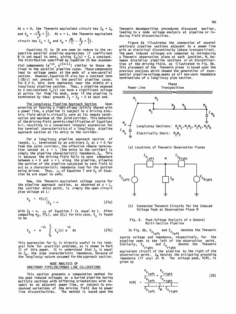
At x = 0, the Thevenin equivalent circuit has Ze = ,oand V.= B( + y At x = L, the Thevenin equivalent
circuit has Z= ZO and V = (BL B+C).
Equations 21 to 26 are seen to reduce to the re-spective parallel pipeline expressions if coefficientB is set equal to zero, giving Ex(s) = C, a constant.The distribution specified by Equation 25 has exponen-
tial components (eYX, ey(xL)) similar to those de-rived in the parallel pipeline cases. These componentslead to voltage peaks at the ends of a non-parallelsection. However,Equation25 also has a constant term(-2B/y) not present in the parallel pipeline cases.For B 7 0, this term dominates near the middle of along/lossy pipeline section. Thus, a pipeline exposedto a non-constant Ex(s) can have a significant voltageat points far from its ends, even if the pipeline isterminated by ideal grounds Z1 = Z2 = 0 at each end.
The Long/Lossy Pipeline Approach Section Uponentering or leaving a right-of-way jointly shared witha power line, a pipeline is subject to a driving elec-tric field whichis virtually zero at its remote termi-nation and maximum at the jointcorridor. This behaviorof thedriving field permits simplification of Equations4-7, resulting in a convenient integral expression forthe terminal characteristics of a long/lossy pipelineapproach section at its entry to the corridor.
For a long/lossy pipeline approach section oflength, L, terminated by an arbitrary Z1 at x = 0 farfrom the joint corridor, the effective remote termina-tion sensed at x = L (the entry to the corridor) issimply the pipeline characteristic impedance,ZO. Thisis because the driving field falls to zero somewherebetween x = 0 and x = L along the pipeline, allowingthe portion of the pipeline subjected to zero field toact as a characteristic impedance load for the portionbeing driven. Thus, p1 of Equation 7 and K1 of Equa-tion 6a are equal to zero.
Now, the Thevenin equivalent voltage source forthe pipeline approach section, as observed at x = L,the corridor entry point, is simply the open circuitpipe voltage at L:
Thevenin decomposition procedures discussed earl i er,leading to a node voltage analysis at pipeline or in-ducing field discontinuities.
Figure 6a illustrates the connection of severalarbitrary pipeline sections adjacent to a power linewith an electrical discontinuity (phase transposition).The peak induced voltages are computed by introducinga Thevenin observation plane at each junction, M, be-tween dissimilar pipeline sections or at discontinui-ties of the driving field, as illustrated in Fig. 6b.This placement of the Thevenin plane is based upon theprevious analyses which showed the generation of expo-nential pipelinevoltagepeaks at all non-zero impedanceterminations of a long/lossy pipe section.
Power LinePhase
Transposition
6
Long/Lossy Sections: M0MlN M1M2N
Electrically Short: M2M3
(a) Locations of Thevenin Observation Planes
VeeLeft ) 0Right
Ve = V(L)|Z2 (27a)
With Zz = 0, p, of Equation 7 is equal to 1. Aftercomputing K2, P L), and Q(L) forthis case, V is foundto be
-yL L rsV = e r E (s) e ds0 o
(27b)
This expression for Ve is directly useful in its inte-gral form for practical problems, as is shown in PartII of this paper. It is understood that Z, is equalto Z, the pipe characteristic impedance, because ofthe %ong/lossy nature assumed fortheapproach section.
NODE ANALYSIS OFARBITRARY PIPELINE/POWER LINE CO-LOCATIONS
This section presents a computation method forthe peak induced voltages on a buried pipelin;e havingmultiple sections with differing orientations with re-spect to an adjacent power line, or subject to pro-nounced variations of the driving field due to powerline discontinuities. The method is based upon the
(b) Connected Thevenin Circuits for the InducedVoltage Peak at Observation Plane M
Fig. 6. Peak-Voltage Analysis of a GeneralMulti-Section Pipeline
In Fig. 6b, V and Za denotes the Theveninleft left
source voltage and impedance, respectively, for thepipeline seen to the left of the observation point.Similarly, V0 and Z0 denote the Thevenin
right -rightequivalent circuit of the pipeline to the right of theobservation point. Zm denotes the mitigating groundingimpedance (if any) at M. The voltage peak, V(M), isgiven by
Vleft +
ZleftV(M) =
Vrightzrg
ori ght(28)
1 1 1
z1 e + YM-+ le0left N right
m0
z m0

786
where Ve and Ze can be obtained from the Thevenin equiv-alent circuits discussed previously.
From Equation 28, JV(M)j can equal zero if either
1) ZM = 0, or (29a)2) Ve Z0 = -V Z . (29b)
eleft right right left
For arbitrary connected buried pipeline sections, Equa-tion 29b is virtually the same as specifying an assem-bled pipeline with constant physical and electricalcharacteristics, spatial orientation, and driving fielddistribution. In other words, an induced voltage peakis expected ona buried pipel ine whereoneof these prop-erties changes abruptly, including the Tflowingp-oints:
1) Junction between a long/lossy parallelsection and a long/lossy non-parallelsection (point M1);
2) Junction between two long/lossy parallelsections having different separationsfrom the power line (points M2 and M3);
3) Adjacent to a power line phase trans-position or a substation where phasingis altered in some way (point M4);
4) Junction between two long/lossy sectionsof differing electrical characteristics,for example, at a high resistivity soil-low resistivity soil transition (point M5);
5) Impedance termination (insulator or groundbed) of a long/lossy section (point M6).
Points M1, M2, M3, and M6 are illustrative of pipelineorientation or termination discontinuities; point M4is illustrativeof a discontinuity of the driving field;and point M5 is illustrative of a discontinuity of thepipeline electrical characteristics. The magnitude ofthe voltage peak at any of these points is computedsimply by applying Equation 28 at the discontinuity tothe Thevenin equivalent circuits for the pipeline sec-tions on either side. In this way, the use of a singlenode equation, along with a collection of Theveninequivalent pipeline circuits, is sufficient to estimatethe voltage peaks on an arbitrary multi-section, buriedpipeline.
COMPUTATION AIDS
IITRI has developed four major programs for theTexas Instruments Model TI-59 programmable hand calcu-lator which permit rapid computation of the drivingelectric field, pipeline characteristics, and Thevenincircuits needed to implement the prediction method ofthis paper. This section briefly summarizes the capa-bilities of each program. Precise details, includingprogram listings and usage instructions, are availablefrom EPRI and AGA in the handbook to be published, ordirectly from IITRI.
Driving Electric Field
Unknown Currents Program This program is usedwhen the currents coupled to multiple earth returnconductors near a power line are strong enough to af-fect the driving field of the pipeline of interest.The conductors may be either power line shield wires,long fence wires, telephone wires, railroad tracks, orother buried pipelines. Since the unknown currentsinfluence each other through mutual coupling, the solu-tion for the currents is obtained by solving a set of
complex-valued simultaneous equations describing theinteractions. The solution algorithm, the Gauss-Seideliterative method, allows the TI-59 to process a systemas complex as five unknown earth return conductors ad-jacent to 25 power line phase conductors, yielding boththe magnitude and phase of each unknown current.
Mutual Impedance Program This program computesthe mutual impedance between adjacent, parallel, earthreturn conductors using Carson's infinite series. Theprogram computes and sums as many terms of the Carsonseries as is required to achieve 0.1% accuracy, usingthe recursive algorithm of Dommel,3 regardless of earthresistivity conditions, conductor configuration (eitheraerial or buried), and conductor separation.
Pipeline Characteristics Program
This program computes the propagation constant, y,and characteristic impedance, ZO, of a buried pipelinehaving arbitrary characteristics. The program can takeinto account the burial depth, pipe diameter, pipe wallthickness, pipe steel relative permeability, pipe steelresistivity, pipe coating resistivity, and earth resis-tivity. The computation method employed for y is aNewton's method solution of the Sunde complex-valuedtranscendental equation; ZO is then computed using theresult for Y.15
Thevenin Circuit Program
This program computes the complex-valued Theveninsource voltage, Ve, and source impedance, Ze for theterminal behavior of an arbitrary earth return conduc-tor subject to a constant driving electric field. Thenature of the conductor is specified for the programsimply by feeding in the conductor's propagation con-stant, y, and characteristic impedance, ZO. The compu-tation method involvesthe solution of Equations llb andllc of this paper.
CONCLUSIONS
This paper has presented a prediction approach forthe voltages induced on gas transmission pipelines by60 Hz ac power lines sharinga joint right-of-way. Thisprediction approach is based upon electrical transmis-sion line theory and allows the characterization ofcomplex features such as pipeline path changes and ter-minations and power line electrical discontinuities.Multiple phase conductors, shield wires, and adjacentgrounded conductors such as railroad tracks and otherpipelines can be accounted for. Advantageous use ismade of a powerful new programmable hand calculator.
The new approach is more accurate than the over-simplified methods now in general use, and yet is stillusable by technicians in the field because ofthesimpleThevenin formulation of voltage peaks and the use ofmagnetic card calculator programs. Field tests, to bediscussed in Part II of this paper, verify the accuracyof the approach when applied to actual joint-use cor-ridors.
REFERENCES
[1] Electrical Transmission and Distribution ReferenceBook, Fourth Edition. Westinghouse Electric Corp.,1964.
[21 "Electromagnetic Effects of Overhead TransmissionLines- Practical Problems, Safeguards, and Methodsof Calculation," by IEEE Working Group on E/M andE/S Effectsof Transmission Lines, IEEE Trans. Pow-er App. Systems, Vol. PAS-94, pp. 892-899,May/June1974.
787
[3] H. W. Dommel et al, Discussion, IEEE Trans. PowerApp. Systems, Vol. PAS-94, pp. 900-904.
[4] Directives Concerning the Protection of Telecommu-nication Lines Against Harmful Effects from Elec-tricity Lines. International Telegraph and Tele-phone Consul tative Committee (CCITT), InternationalTelecommunications Union, 1962 (supplemented 1965).
[5] A. W. Peabody and A. L. Verhiel, "The Effects ofHigh Voltage Alternating Current (HVAC) Transmis-sion Lines on Buried Pipelines," Paper No. PCI-70-32 presentedat IEEE/IGA Petroleum and ChemicalIndustry Conference, Tul sa, Oklahoma, 15 September1970.
[6] C. G. Siegfried, "AC Induced Interference on Pipe-lines," presented at Interpipe 73 Conference,Houston, Texas, 31 October 1973.
[7] C. A. Royce, "Alternating Current Problems ofPipelines," presented at A.G.A. Operating SectionTransmission Conference, Houston, Texas, 18 May1971.
[8] E. C. Paver, Sr., "The Effects of Induced Currenton a Pipeline," Paper No. 54 presented at NACE26th Annual Conference, Philadelphia, Pa., 2-6March 1970.
[9] M. A. Puschel, "Power Lines and Pipelines in CloseProximity During Construction and Operation," Ma-terials Performance, Vol. 12, pp. 28-32, December1973.
[10] Technical Compatibility Factors for Joint-UseRights-of-Way (for Bureau of Land Management,Contract 08550-CT5-5). Aerospace Corp., 1 Feb-ruary 1975.
[11] J. Pohl, "Influence of High-Voltage Overhead Lineson Covered Pipelines," Paper No. 326 presented atCIGRE, Paris, France, June 1966.
[12] B. Favez and J. C. Gougeuil, "Contribution to Stud-ies on Problems Resulting from the Proximity ofOverheadLines with Underground Metal Pipe Lines,"Paper No. 336 presented at CIGRE, Paris, France,June 1966.
[13] D. N. Gideon et al., Final Report on Project San-guine. Parametric Study of Costs for InterferenceMiti gation in Pi pelines (to IIT Research Institute).Battel le Col umbus Laboratories, Columbus, Ohio,30 September 1971.
[14] J. R. Sherbundy, The Effects of High Voltage Over-head Transmission Lines on Underground Pipelines.M.S. Thesis, Department of Electrical Engineering,Ohio State University, 1975.
[15] E. D. Sunde, Earth Conduction Effects in Transmis-sion Systems, New York: Dover Publications, 1968,pp. 14-16 and pp. 146-149.
[16] E. F. Vance, DNA Handbook Revision, Chapter 11,Coupling to Cables (for Dept. of the Army, Con-tract DAAG39-74-C-0086). Stanford Research In-stitute, Menlo Park, CA., December 1974
For Combined Discussion, see page 791
IEEE Transactions on Power Apparatus and Systems, Vol. PAS-98, No. 3 May/June 1979
PREDICTION METHOD FOR BURIED PIPELINE VOLTAGESDUE TO 60 Hz AC INDUCTIVE COUPLINGPART II -- FIELD TEST VERIFICATION
John Dabkowski Allen Taflove, Member, IEEEIIT Research Institute10 West 35th Street
Chicago, Illinois 60616
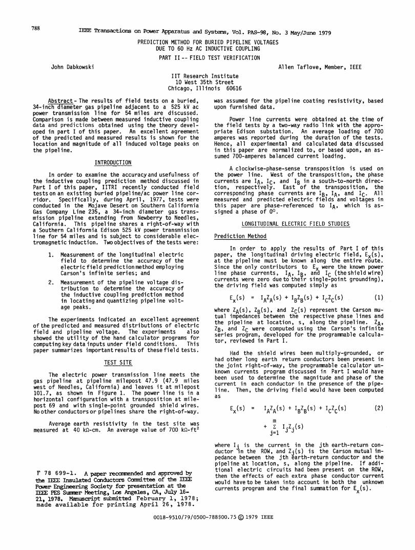
Abstract- The results of field tests on a buried,34-inch diameter gas pipeline adjacent to a 525 kV acpower transmission line for 54 miles are discussed.Comparison is made between measured inductive couplingdata and predictions obtained using the theory devel-oped in part I of this paper. An excellent agreementof the predicted and measured results is shown for thelocation and magnitude of all induced voltage peaks onthe pipeline.
INTRODUCTION
In order to examine the accuracyand usefulness ofthe inductive coupling prediction method discussed inPart I of this paper, IITRI recently conducted fieldtestsonan existing buried pipeline/ac power line cor-ridor. Specifically, during April, 1977, tests wereconducted in the Mojave Desert on Southern CaliforniaGas Company Line 235, a 34-inch diameter gas trans-mission pipeline extending from Newberry to Needles,California. This pipeline shares a right-of-way witha Southern California Edison 525 kV power transmissionline for 54 miles and is subject to considerable elec-tromagnetic induction. Two objectives of the tests were:
1. Measurement of the longitudinal electricfield to determine the accuracy of theelectric field predictionmethod employingCarson's infinite series; and
2. Measurement of the pipeline voltage dis-tribution to determine the accuracy ofthe inductive coupling prediction methodi n locati ng and quanti zi ng pi pel i ne vol t-age peaks.
The experiments indicated an excellent agreementof the predicted and measured distributions of electricfield and pipeline voltage. The experiments alsoshowed the utility of the hand calculator programs forcomputing key data inputs under field conditions. Thispaper summarizes important results of these field tests.
TEST SITE
The electric power transmission line meets thegas pipeline at pipeline milepost 47.9 (47.9 mileswest of Needles, California) and leaves it at milepost101.7, as shown in Figure 1. The power line is in ahorizontal configuration with a transposition at mile-post 69 and with single-point grounded shield wires.No other conductors or pipelines share the right-of-way.
Average earth resistivity in the test site wasmeasured at 40 kQ-cm. An average value of 700 ko-ft2
F 78 699-1. A paper recamnended and approved bythe IEEInsulated Ccnductors Canmittee of the IEEEPower Engineering Society for presentation at theIEEE PES Summer Meeting, Los Angeles, CA, July 16-21, 1978. Manuscript submitted February 1, 1978;made available for printing April 26, 1978.
was assumed for the pipeline coating resistivity, basedupon furnished data.
Power line currents were obtained at the time ofthe field tests by a two-way radio link with the appro-priate Edison substation. An average loading of 700amperes was reported during the duration of the tests.Hence, all experimental and calculated data discussedin this paper are normalized to, or based upon, an as-sumed 700-amperes balanced current loading.
A clockwise-phase-sense transposition is used onthe power line. West of the transposition, the phasecurrents are IA' IC, and IB in a south-to-north direc-tion, respectively. East of the transposition, thecorresponding phase currents are IB, IA, and IC. Allmeasured and predicted electric fields and voltages inthis paper are phase-referenced to IA, which is as-signed a phase of 00.
LONGITUDINAL ELECTRIC FIELD STUDIES
Prediction Method
In order to apply the results of Part I of thispaper, the longitudinal driving electric field, Ex(s),at the pipeline must be known along the entire route.Since the only contributors to Ex were the known powerline phase currents, IA, I$, and IC (theshieldwire)currents were zero due to their single-point grounding),the driving field was computed simply as
Ex(s) = IAZA(S) + IBZB(s) + ICZC(s) (1)where ZA(s), ZB(s), and Zc(s) represent the Carson mu-tual impedances between the respective phase lines andthe pipeline at location, s, along the pipeline. ZASZB, and ZC were computed using the Carson's infiniteseries program, developed for the programmable calcula-tor, reviewed in Part I.
Had the shield wires been multiply-grounded, orhad other long earth return conductors been present inthe joint right-of-way, the programmable calculator un-known currents program discussed in Part I would havebeen used to determine the magnitude and phase of thecurrent in each conductor in the presence of the pipe-line. Then, the driving field would have been computedas
Ex(s) = IAZA(s) + IBZB(S) + ICZC(s) (2)m
+ z I.Z.(s)j=1 J J
where Ij is the current in the jth earth-return con-ductor in the ROW, and Zj(s) is the Carson mutual im-pedance between the jth earth-return conductor and thepipeline at location, s, along the pipeline. If addi-tional electric circuits had been present on the ROW,then the effects of each extra phase conductor currentwould haveto be taken into account in both the unknowncurrents program and the final summation for EX(s).
0018-9510/79/0500-788$00.75 0 1979 IEEE
788
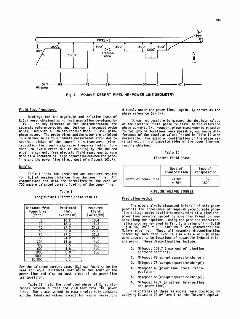
Fig. I MOJAVE DESERT PIPELINE- POWER LINE GEOMETRY
Field Test Procedures
Readings for the magnitude and relative phase ofEx(s) were obtained using instrumentation developed byIITRI. The key elements of the instrumentation areseparate reference-point and test-point grounded probewires, used with a Hewlett-Packard Model HP 3575 gain-phase meter. The probe wires andthemeter are shieldedin a manner so as to eliminate measurement error due tospurious pickup of the power line's transverse (elec-trostatic) field and stray radio frequencyfields. Fur-ther, to avoid error due to coupling by the inducedpipeline current, free electric field measurements weremade at a location of large separation between the pipe-line and the power line (i.e., west of milepost 101.7).
Resul ts
Table I lists the predicted and measured resultsfor |EXI at varying distances from the power line. Allcomputations and data are normalized to the case of700 ampere balanced current loading of the power line.
Table I
Longitudinal Electric Field Results
Distance from Predicted MeasuredPower Line Field Field
(feet) (volts/km) (volts/km)0 10.2 10.4
20 18.3 14.340 27.3 24.560 29.0 27.080 27.2 22.2100 24.2 22.2200 14.0 14.0300 9.5 8.5600 4.8 4.01000 2.9 1.65000 0.4
10,000 i 0.1
For the balanced current case, lExl was found to be thesame for equal distances both north and south of thepower line and also on both sides of the power linetransposition.
Table II lists the predicted phase of E at dis-tances between 60 feet and 2000 feet from tAe powerline. The phase tended to remain relatively constantat the tabulated values except for rapid variations
directly under the power line. Again, IA serves as thephase reference (4= 00).
It was not possible to measure the absolute valuesof the electric field phase relative to the referencephase current, IA. However, phase measurements relativeto two ground locations were possible, and hence dif-ferences of the absolute values listed in Table II weremeasurable. For example, confirmation of the phase re-versal occurringon opposite sides of the power line wasreadily obtained
Table IIElectric Field Phase
West ofTransposi tion
East ofTransposition
-1200 00+ 600 1800
PIPELINE VOLTAGE STUDIES
Prediction Method
The node analysis discussed in Part I of this paperpredicts the appearance of separably-calculable pipe-line voltage peaks atall discontinuities of a pipeline-power line geometry spaced by more than 2/Real (y) me-ters along the pipeline. Using the pipeline character-istics program reviewed in Part I, a value ofy= (0.115+ j 0.096) km-1 = 0.15 /400 km- 1 was computed for theMojave pipeline. Thus, all geometry discontinuitiesspaced by more than (2/0.115) km = 17.4 km 10 mileswere assumed to be locations of separable induced volt-age peaks. These discontinuities include:
1. Milepost 101.7 (near end of pipelineapproach section);
2. Milepost 89 (abrupt separation change);3. Milepost 78 (abrupt separation change);4. Milepost 69 (power line phase trans-
position);5. Mil epost 55 (abrupt separation change);6. Milepost 47.9 (pipeline intersecting
the power line).The voltages at these mileposts were predicted by
applying Equation 28 of Part I to the Thevenin equiva-
789
L-
-101.7- 89Milepost
47.9

790
lent pipeline circuits observed at each point. Assum-ing that the pipeline characteristics y and ZO wereconstant with position along the pipeline, Zeleft andZOHriht observed at each Thevenin plane were set con-stant at the value ZO (due to the long/lossy nature ofthe adjacent pipe sections). Further, ZM was assumed toequal infinity at each Thevenin plane because no acmitigation grounds were connected at the time to thepipeline. Equation 28 was thus simplified to
V(M) = V 2left Veright (3a)
For the important special case where the drivingelectric field had a step discontinuity at M, that is,Ex(M+) = Elet and ExYM-)= Eright, Equation 3a can befurther simplified to
V2(M)= r[ ) + yE )]
giving
IV(M)l = eft Erightl = E l21y I~
the power line occurs at a fixed pipeline-power lineseparation of 300 feet. From Tables I and II, Eleft9.5/-1200 vol ts/km and Eright 9.5 /00 volts/km, glving
IV(69)I1 3.33 *1(9.5 /-1200)- (9.5 /00)1- 54,8 vol ts (7)
Milepost 55: By a few miles west of milepost 55,the lateral separation has gradually increased to ap-proximately 500 feet. At Milepost 55 there isan abruptdiscontinuity wherethe lateral separation becomes about1200 feet. From Tables I and II,
Eleft - EX15001 = 5.8 /00 volts/km, and
Eright - Ex11200' 2.4 /00 volts/km, giving
IV(55)1 3.33 1(5.8 /0°) - (2.4 /00)1(3b)
In Equations 3a - 3c, the definition and sign of V fand VQrioht were taken from Figure 5b of Part I, ersubstituting the computed value of IyI = 0.15 km1, thefinal form of the peak voltage prediction equation was
IV(M) I = = 3.331AE(M)I. (3d)0.3
To illustrate this computational approach, the pre-dicted voltage peaks are calculated using Equation 3d,starting at the west end of the shared right-of-way.
Milepost 101.7: The first discontinuity occurshere because the power line approaches the pipeline toa distance of 200 feet. The angle of approach is 450and, in general, it will be found that for angles great-er than 15° to 200 that the drop-off in electric fieldstrength with increasing distance from the power lineis sufficiently fast so that the contribution to theobservation point voltage from the approaching leg issmall, as may be verified by performing a trapezoidalintegrationof Equation 27b Qf Part I. Hence, Eleft 0and Eright EX1200' = 14.0 /-1200 Volts/km (from Ta-bles I and II), giving
IV(101.7)1 = 3.33 * 114.0 /-1200) - 0146.6 volts (4)
Milepost 89: The next discontinuity is a resultof the pipeline-power line separation increasing toabout 3500 feet in the 78 to 89 mile region. From Ta-bles I and II, E1 ExI200' 14.0 /-1200 volts/kmand Eright Ex 1356t 0.6 /-1200 volts/km, giving
IV(89)I 3.33 * 1(14.0 /-1200) - (0.6 /-.1200)I44.6 volts (5)
Milepost 78: At this point, the pipeline-powerline separation decreases to about 300 feet. From Ta-bles I and II, Eleft E 13500' 0.6 /-1200 volts/kmand Eright - Ex13001 9.9 /-1200 volts/km, giving
IV(78)I1 3.33 1(0.6 /-1200) - (9.5 /-1200)1= 29.6 volts (6)
Milepost 69: At this point, a transposition of
11.3 volts (8)
Milepost 47.9; The power line and pipeline ap-proach this point from the west at a separation of ap-proximately 300 feet. At mile 47.9, the power linecrosses the pipeline at an angle of about 220, and con-tinues onward. Similar to the case at Milepost 101.7,the drop-off in electric field strength with increasingdistance from the power line is sufficiently fast sothat the contribution to the observation point voltagefrom the departing leg is small. Hence, E ht 0 andEleft E1300 = 9.5 /00volts/km (from Table r and II,giving 3.300
IV(47.9)1 3.33 1(9.5 /00) - 01- 31.6 volts (9)
Field Test Results
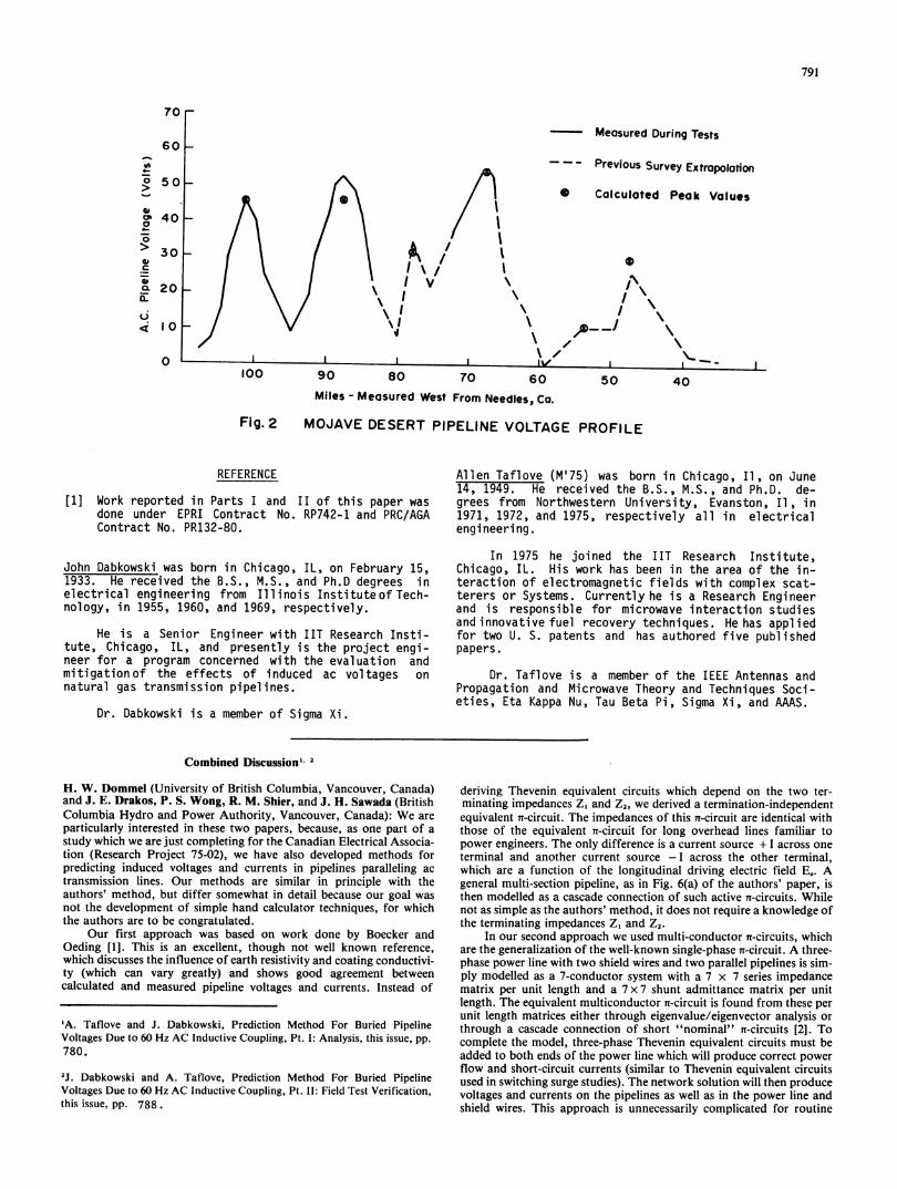
Figure 2 plotsboththe measured ac voltage profileof the Mojave pipeline and the computed voltage peaks.The solid curve represents voltages measured by IITRI;the dashed curve is a set of data (normalized to 700amperes power line current) obtained by a SouthernCalifornia Gas Company survey in December 1976.
From Figure 2, it is apparent that the predictionmethod of this paper succeeded in locating and quantiz-ing each of the pipeline voltage peaks with an error ofless than + 20%. Considering the effects of finely-detailed ground resistivity non-uniformities and cou-pling between adjacent discontinuities (not accountedfor when using the Thevenin node analysis of long/lossysections), this level of accuracy is sufficient for manyengineering purposes and greatly exceeds that of pre-vious available approaches.
CONCLUSIONS
Experimental verification has been obtained for thepeak-inductive-coupling prediction method of Part I ofthis paper. Locations of induced voltage peaks on bur-ied pipelines are readily identifiable and their magni-tudes calculable with an accuracy not obtainable pre-viously.
As shown, the peak-voltage calculations for theMojave pipeline are quite simple. This is due to thefact that successive pipeline/powerlinediscontinuitieswere spaced far enough apart to minimize their inter-action. Ina dense urban environment, this would not bethe case. Here, the cal cul ations would become more com-plex, but voltage prediction in this situation wouldstill be within the scope of the distributed sourcetheory and programmable calculator programs developedin Part I of this paper.
791
70 r
Measured During Tests60p-
- - - Previous Survey Extrapolation
0 Calculated Peak Values
0D
A---1N
\- IV IX
90 80 70 60 50 40
-
Miles - Measured West From Needles, Ca.
Fig. 2 MOJAVE DESERT PIPELINE VOLTAGE PROFILE
REFERENCE
[1] Work reported in Parts I and II of this paper wasdone under EPRI Contract No. RP742-1 and PRC/AGAContract No. PR132-80.
John Dabkowski was born in Chicago, IL, on February 15,1933. He received the B.S., M.S., and Ph.D degrees inelectrical engineering from Illinois Instituteof Tech-nology, in 1955, 1960, and 1969, respectively.
He is a Senior Engineer with IIT Research Insti-tute, Chicago, IL, and presently is the project engi-neer for a program concerned with the evaluation andmitigationof the effects of induced ac voltages onnatural gas transmission pipelines.
Dr. Dabkowski is a member of Sigma Xi.
Allen Taflove (M'75) was born in Chicago, II, on June14, 1949. He received the B.S., M.S., and Ph.D. de-grees from Northwestern University, Evanston, II, in1971, 1972, and 1975, respectively all in electricalengineering.
In 1975 he joined the IIT Research Institute,Chicago, IL. His work has been in the area of the in-teraction of electromagnetic fields with complex scat-terers or Systems. Currently he is a Research Engineerand is responsible for microwave interaction studiesand i nnovati ve fuel recovery techni ques. He has appl i edfor two U. S. patents and has authored five publishedpapers.
Dr. Taflove is a member of the IEEE Antennas andPropagation and Microwave Theory and Techniques Soci-eties, Eta Kappa Nu, Tau Beta Pi, Sigma Xi, and AAAS.
Combined Discussion" 2
H. W. Dommel (University of British Columbia, Vancouver, Canada)and J. E. Drakos, P. S. Wong, R. M. Shier, and J. H. Sawada (BritishColumbia Hydro and Power Authority, Vancouver, Canada): We areparticularly interested in these two papers, because, as one part of astudy which we are just completing for the Canadian Electrical Associa-tion (Research Project 75-02), we have also developed methods forpredicting induced voltages and currents in pipelines paralleling actransmission lines. Our methods are similar in principle with theauthors' method, but differ somewhat in detail because our goal wasnot the development of simple hand calculator techniques, for whichthe authors are to be congratulated.
Our first approach was based on work done by Boecker andOeding [1]. This is an excellent, though not well known reference,which discusses the influence of earth resistivity and coating conductivi-ty (which can vary greatly) and shows good agreement betweencalculated and measured pipeline voltages and currents. Instead of
'A. Taflove and J. Dabkowski, Prediction Method For Buried PipelineVoltages Due to 60 Hz AC Inductive Coupling, Pt. I: Analysis, this issue, pp.780.
2J. Dabkowski and A. Taflove, Prediction Method For Buried PipelineVoltages Due to 60 Hz AC Inductive Coupling, Pt. Il: Field Test Verification,this issue, pp. 788.
deriving Thevenin equivalent circuits which depend on the two ter-minating impedances Z, and Z2, we derived a termination-inde-pendentequivalent n-circuit. The impedances of this n-circuit are identical withthose of the equivalent n-circuit for long overhead lines familiar topower engineers. The only difference is a current source + I across oneterminal and another current source - I across the other terminal,which are a function of the longitudinal driving electric field E.. Ageneral multi-section pipeline, as in Fig. 6(a) of the authors' paper, isthen modelled as a cascade connection of such active n-circuits. Whilenot as simple as the authors' method, it does not require a knowledge ofthe terminating impedances Z, and Z2.
In our second approach we used multi-conductor n-circuits, whichare the generalization of the well-known single-phase n-circuit. A three-phase power line with two shield wires and two parallel pipelines is sim-ply modelled as a 7-conductor system with a 7 x 7 series impedancematrix per unit length and a 7 x 7 shunt admittance matrix per unitlength. The equivalent multiconductor n-circuit is found from these perunit length matrices either through eigenvalue/eigenvector analysis orthrough a cascade connection of short "nominal" n-circuits [2]. Tocomplete the model, three-phase Thevenin equivalent circuits must beadded to both ends of the power line which will produce correct powerflow and short-circuit currents (similar to Thevenin equivalent circuitsused in switching surge studies). The network solution will then producevoltages and currents on the pipelines as well as in the power line andshield wires. This approach is unnecessarily complicated for routine
%A0-
> 50
Ol 40
30> 30._
0.
4 10
oj
_-
_
I
I^V/ t!'I
'I
100- l~~~I
I I I
\
792studies, but it is well suited for analyzing transient conditions.Preliminary studies have shown that fairly high voltages may be induc-ed in the pipeline during power line switching (e.g., during normalenergization). Since frequencies up to a few kHz are involved in swit-ching surges, the equivalent n-circuit must be replaced by cascade con-nections of short nominal multiconductor n-circuits in this case, withthe section length typically in the order of 0.08 km. Approximatemodelling of the frequency dependence of line parameters did notchange the switching-surge-induced overvoltages significantly.
Would it be easy for the authors to calculate currents in thepipeline as well? Currents in the pipe may be of concern if a single-line-to-ground fault occurs on the power line, where 30% or more ofthe fault current may return through the pipe. Do the authors foreseeany convergence difficulties in the "Unknown Currents Program" ifthe number of unknown currents gets close to the upper limit of 5?Gauss elimination would be direct, of course, but may no longer fit intoprogrammable hand calculators.
One of the key parameters affecting pipeline induced voltages is thepipeline shunt conductance per unit length, which has two series com-ponents-the coating conductance per unit length and the earth con-ductance per unit length. The authors refer to a "coating resistivity" of700 kQ * ft2. Does this mean that the resistance through one square footof coating is 700kQ, or is this actually the resistivity value of the coatingbut with units of kQ ft?. If the former applies, the coating conduc-tance per unit length of pipeline turns out to be about 0.04 mS/m.Could the authors give more details on the test procedure used to deter-mine the value of 700 kQ ft2, and also give a description of thecoating?
Inserting the value of earth resistivity of 400 Q - m and the dc com-ponent of the author's value of y into Sunde's expression for the earthconductance per unit length yields a value of about 0.8 mS/m. Therelative magnitudes of coating and earth conductances per unit lengthindicate a well coated pipeline. However, in some cases the coating con-ductance per unit length may be large with respect to the earth conduc-tance per unit length, e.g. where the coating is poor or the earthresistivity is high. In these cases only a portion of the total ac voltagefrom pipeline to remote earth appears across the coating. The expectedvoltage from pipeline to near earth should then be obtained by takingthe total calculated voltage and apportioning it across the coating andearth conductances. Have the authors made field tests where thismodification was required?
REFERENCES
[1 H. Boecker and D. Oeding, "Induced voltages in pipelines on theright-of-way of high voltage lines (in German), "Elektrizitatswirt-schaft", vol. 65, pp. 157-170, 1966.
[21 User's manual for program "Line Constants of Overhead Lines",Bonneville Power Administration, June 1972.
Manuscript received August 15, 1978.
Luke Yu (The Ralph M. Parsons Company, Pasadena, CA): Theauthors are to be commended for presenting two fine articles regardingthe induced voltage in buried pipeline from a nearby A.C. powertransmission line. This phenomena became more significant at the ad-vent of EHV or UHV power transmissions. Upon having gone withgreat interest through the papers, I would like to express my viewpointsand raise some queries:
1. In order to determine the interference between an overhead A.C.power line and an adjacent above-ground communication circuit, arigorous method should take into account the distributed inductive andcapacitive couplings as well as the line terminations of both systems. Ifound that a hugh discrepancy exists between the computed results bas-ed on a rigorous approach and on a simple method which takes intoconsideration the mutual inductive coupling only for a sample study.
2. Ex(s), the driving field appears to be the governing factor indetermining the induced pipeline voltage. However, as shown in Equa-tion (1) of Part II, Ex(s) is simply computed from the products of linecurrents and mutual impedances. It appears to me a more precise ap-proach should be adopted in determining Ex(s). In fact, the line cur-rents vary along the lines especially for long EHV or UHV powertransmission lines.
3. As shown in Table I of Part II, the predicted field values and themeasured field data appear in general to be pretty close. However, thereare certain degrees of discrepancy between them with respect to dif-ferent distances. In my opinion the study of induced pipeline voltage
should take the pipeline as a part of the whole electrical system in theanalysis as well as A.C. power lines because they are electrically in-terlinked and form a complete system. All the unknowns should besolved simultaneously. The authors' comments are appreciated.
Manuscript received August 14, 1978.
Donald C. Anderson (Southern California Gas Company, Los Angeles,CA): Figure 1 showing the Mohave Desert pipeline-power line geometryis a simplified depiction of the actual spatial relationships between thefacilities. At Milepost 89 the power line actually recedes from thepipeline at an angle of approximately 4°. This is not the same as theabrupt separation change depicted in Figure 1 and treated as suchmathematically in equation (5), i.e., Eright EX13500' - 0.6 L - 1200volts/km (from Table 1). Recognition of the shallow angle at which thepower line recedes from the pipeline beginning at Milepost 89 would ap-pear to result in a lower predicted voltage at Milepost 89 but asignificantly higher voltage easterly of Milepost 89. This seems to beconsistent with the voltage pattern measured during the tests, as shownin Figure 2. Assistance in how to treat less than abrupt separationchanges in the context of the prediction method would be appreciated.
At Milepost 78, E,,f, is shown as approximately equal to E.j3500' -
0.6 L - 120° volts/km. Since the approach angle at the point of obser-vation is 900 (Figure 1) and a lesser but still significant angle in the field,I wonder why E,,f, is not shown as equal to zero. This would result in aslightly higher predicted voltage at Milepost 78, which again appears tobe consistent with the voltages measured during the tests. Further, forMilepost 101. 7 and Milepost 47.9, E,ft and E,ight respectively are shownas zero because "the drop-off in electrical field strength with increasingdistance from the power line is sufficiently fast so that the contributionto the observation point voltage from the approaching/departing leg issmall". A reason for the different treatment of essentially similar ap-proach angles would be appreciated.
Manuscript received August 14. 1978.
R. E. Aker (Southern California Edison Co., Rosemead, CA): Theauthors are commended for their contributions to the distributed sourceanalysis approach to the prediction of induced voltages on buriedpipelines.
Perhaps the derivation of Equation I Ic would be clearer if it wasnoted that Equations 10 and 1 lb are substituted into Equation 1 la toget Equation 1 lc. This derivation also leads to the determination of theload current through the terminating impedance:I(0) = V(0)/Z, = Eo/y [2Z2 - (Z2 + ZO)eYL - (Z2 - Zo)evL]/[(Z1 + ZJ) (Z2 + ZJ)eYL - (Z, - ZJ) (Z2 - Zo)e-yl.
A transposition in a power line adjacent to a pipeline is an in-teresting case where the transposition could induce a peak voltage ontothe pipeline. This paper indicates that even a mere phase shift in thedriving electric field, due to the transposition, induces a peak voltagewhere one might expect a nullifying effect.
The Southern California Edison Company is applying thisdistributed source analysis approach to various transmission line pro-jects. Edison's proposed 240 mile long Devers-Palo Verde 525kVTransmission Line is expected to parallel approximately 100 miles ofseveral sections of buried pipeline. The analysis presently indicates thata peak voltage of up to 300 volts could be induced at the insulated ter-minals of some of these sections.
Manuscript received August 1, 1978.
Adrian L. Verhiel (Trans Mountain Pipe Line Company Ltd., Van-couver, B.C.): I commend the authors for this interesting and signifi-cant research on the methods developed to predict the potentials thatmay result from 60 Hz-A.C. induction coupling in buried pipelines.For over 10 years, we have carried out tests and measurements on theseproblems with very marginal results due to inadequate basic research.
The induced potential, being a function of the pipeline propaga-tion constant y and the characteristic impedance Zo are both dependenton pipeline resistance. The methods of induced potential calculationsapply to gas pipelines, normally of constant wall thickness. What wouldbe the effect if applied to liquid pipelines with large varying wallthicknesses in relative short distances?

In remote areas where commercial electric power is noteconomically available, cathodic protection for the pipelines may besupplied by sacrificial anode systems. The latter may be of thedistributed anode type or of the concentrated anode bed variety. Whatwould be the effect of the various point grounds on the induced poten-tial?
In determining the pipeline characteristics, it appears that onlysingle pipeline cases have been considered. What would be the effect onmultiple pipelines in the same right-of-way? The electrical constants ofthe pipeline characteristics could vary considerably due to the pipelines'mutual impedance and it is wondered if future consideration will begiven to this part of the problem. Table I under "Results" may requiresome clarification as to the distance from the powerline.
The authors have laid a very important foundation for calculatinginduced potential effects on buried pipelines and it is hoped that furtherresearch will be carried out to enable the pipeline industry to calculatethe effects mentioned above and to develop the necessary mitigationmethods.
It is now up to the industry to apply the suggested methods andreport the findings for varification.
Manuscript received June 26, 1978.
Allen Taflove and John Dabkowski: The authors thank the discussorsfor their comments and interest in the companion papers. The questionsfor each of the prepared discussions will be addressed in turn.
In reply to the question from Mr. A. L. Verhiel, the followingcomments are offered.
1) If the wall-thickness variations of liquid-carrying pipelines occur
in short distances relative to 2/Real (y), the effect of the variations uponthe induced pipeline potential is greatly smoothed. In effect, for thiscase, choosing an average value of pipe thickness is sufficiently ac-
curate. If, however, variations in wall thickness occurs at much longerintervals [comparable to or greater than 2/Real (y)], the node analysisshould be applied using the particular value of wall thickness to deter-mine the induced voltage peak at that point. The analysis is valid forboth liquid and natural gas transmission and distribution pipelines.
2) Point grounds located at large intervals [comparable to 2/Real(y)] can be accounted for by applying the node analysis at the locationof each point ground, using as a value of ZM of Figure 6 and Equation28 the value of the ac grounding impedance of the ground bed. Ingeneral, if ZM is small compared to ZO of the pipeline, mitigation of in-duced pipeline voltages will be achieved within an interval of 2/Real (y)of the ground bed. Now, if a distributed anode system is installed, i.e.,if point grounds are connected at very small intervals relative to 2/Real(y), the principal effect of the grounds is to increase the effectiveaverage admittance of the pipeline coating and thus increase themagnitude of y. Here, the relative increase in pipeline mitigation, ob-tained for the entire length of the distributed anode system, can bedetermined by computing the magnitude of y before and after the in-stallation, and forming the ratio of the computed magnitudes.
3) Although this paper deals only with the single pipeline case (forsimplicity), multiple pipelines in the same right-of-way can be accom-
modated by the analysis. For most cases of pipeline coating quality,earth resistivity, and separation between adjacent pipelines, it can beshown that the mutual impedance between pipelines is dominated bythe inductive component, calculable by Carson's series, rather than theresistive component, due to the direct interchange of pipe currents
through the earth. Thus, the Unknown Currents Program, discussedunder the heading Computation Aids, can be used with accuracy tocompute the mutual effects between as many as five pipelines in thesame right-of-way. A more detailed description of this case is containedin the reference book to be published.
4) In Table I of Part II, the distance from the power line ismeasured from the center phase conductor.
The following comments are provided to the discussion of Mr. R.E. Aker.
1) Equations I1 a, 1 lb, and 1 lc of Part I are in fact a direct decom-position of Equation 10 for the case x = 0. The purpose of performingthis decomposition is to prove that the terminal behavior of a pipelinecan be represented by a Thevenin equivalent-circuit where the effects ofinducing field, pipeline characteristics, and load impedances can beconveniently separated.
2) As noted, a key consequence of the theory is the importance ofthe phase of the inducing field. In particular, rapid shifts of the phasewith distance along the pipeline lead to pronounced induced pipelinevoltge peaks.
793
The following comments are provided to the discussion of Messrs.Dommel, Drakos, Wong, Shier, and Sawada.
1) Unless one is at a large distance (> 2/Rey) from an end, it is notclear how the discussors can dispense with knowledge of the pipelineterminating impedances, Z, and Z2, in determining induced pipelinevoltages using the approach of Boecker and Oeding. Z1 and Z2 canrange from very high values (for insulator terminations) to very lowvalues (for ground-bed terminations) and are shown by the distributedsource analysis approach to definitely affect the position and magnitudeof pipeline voltage peaks.
2) Currents in a pipeline are computed using Equation 4a of Part I.The simplification of this equation was not pursued in the paperbecause the emphasis was on induced pipeline voltages. The authorsacknowledge that pipeline currents may be of concern during fault con-ditions. An approximate value of the maximum induced pipeline cur-rent can be obtained by applying the Unknown Currents Program,discussed in the section Computation Aids.
3) The authors foresee no convergence difficulties in the UnknownCurrents Program if the number of unknown currents gets close to theupper limit of 5. The upper limit here is determined solely by thememory limits of the calculator used. The basic Gauss-Seidel solutionalgorithm is well known and has been used successfully to solvemuch larger systems of equations.
4) The pipeline coating resistivity means the resistance observedthrough one square foot of coating. The coating resistance was notdirectly measured by the authors. The value given is estimated from avalue measured at the time of pipe installation which was adjusted totake into account subsequent deterioration. This latter factor wasestimated on the basis of the increase in time of the impressed cathodicprotection current required to maintain a constant pipe-to-soil poten-tial. Details of the coating composition are unknown to the authors.
5) For a good coating, as in this case, the total ac voltage from thepipeline to remote earth appears essentially across the coating. Situa-tions have been encountered on other pipelines where current leakagefrom the pipe was significant and care had to be taken in obtaining atrue remote earth termination for the measurement voltmeter.
The following comments are provided to the discussion of Mr.D.C. Anderson.
1) The authors have found that a pipeline section receding from anac power line at virtually any angle greater than 00 develops only a smallvalue of Thevenin source voltage, Vy, observed at the point of closestapproach to the power line. A good rule of thumb is that VO can be setto zero for pipe sections having recession angles exceeding Real (y) x100, where y is the pipeline propagation constant taken in units of km-1.Essentially, at angles larger than this, only an electrically short sectionof the receding pipeline is subject to an appreciable driving electricfield, resulting in a relatively small voltage contribution of the entirereceding section. Thus, in the paper, all angled pipeline sections wereconsidered to essentially develop a zero voltage contribution since allhad recession angles exceeding Real (y) x 100 = 0.115 x 10° = 10.
2) Use of this assumption is relatively obvious for the calculationsmade at Mileposts 101.7 and 47.9. At both locations the pipeline com-pletely receded from the power line. At Mileposts 89 and 78, thepipeline receded from the power line a large but still finite distance.Hence, a small but larger than zero contribution to the induced voltagecould be expected from the receding sections. An approximate methodto take this into account, as used in the paper, thus yielded non-zerovalues for Er,gh, at Milepost 89 and E,f, at Milepost 78, respectively. Amore detailed and rigorous discussion of the treatment of the Thevenincharacterization of pipeline departure and approach sections is contain-ed in the reference book to be published. The main attempt of thematerial presented in this paper was to establish the concept that avoltage peak on the pipeline can be expected at a location of an electricfield discontinuity.
The following comments are provided to the discussion of Mr. L.Yu.
1) The paper dealt only with inductive coupling to buried pipelines,and not to above-ground communications circuits. Capacitive couplingto buried pipelines is negligible.
2) Part II of the paper dealt only with a single verification case in-volving a simple right-of-way containing one ac power line and onepipeline. Here, E. (s) can be taken simply as a summation of the pro-ducts of line currents and mutual impedances. However, as explained inPart I, the analysis is sufficiently general to take into account thepresence of multiple conductors in the right-of-way, such as pipelines,shield wires, and railroad tracks. The Unknown Currents Program,summarized in the section Computation Aids, can account for the

794mutual interaction between up to five long earth-return conductors in Another way of looking at this situation is that the phase currents arethe right-of-way. This program has been used successfully in a number provided by a voltage source with a very low source impedance relativeof other case history tests involving much more complicated rights-of- to the Carson mutual impedance between the phase conductors and theway than that discussed in Part 11. Full description of these case pipeline. The authors believe that solving for the phase currentshistories and the usage of all of the computation aids is contained in the simultaneously with the pipe current introduces needless complicationreference book to be published. in this situation, given the added work involved and the marginal in-3) Under the non-fault conditions discussed in the paper, the authors crease in accuray. However, this is not the case during power line faulthave found that the induced current in pipelines buried near ac power conditions when 30% or more of the fault current may return throughlines has a limit of about 5% of the typical phase conductor current. the pipe due to earth current effects as well as Carson-type coupling.The reaction of this pipeline current back to the phase conductor cur- Here, accuracy demands a simultaneous solution of all currents.rents is typically small enough so that, for all practical purposes, thephase currents can be treated as being unaffected by the pipe current. Manuscript received October 16, 1978.