IEEE JOURNAL ON SELECTED AREAS IN COMMUNICATIONS (ACCEPTED JUNE 30, 2016) 1

Dynamic Resource Allocation for Smart-GridPowered MIMO Downlink Transmissions

Xin Wang, Senior Member, IEEE, Tianyi Chen, Xiaojing Chen, Student Member, IEEE,Xiaolin Zhou, Member, IEEE and Georgios B. Giannakis, Fellow, IEEE

Abstract—Benefiting from technological advances in the smartgrid era, next-generation multi-input multi-output (MIMO) com-munication systems are expected to be powered by renewableenergy sources (RES) integrated in the distribution grid, thusrealizing the vision of “green communications.” However, pene-tration of renewables introduces variabilities in the traditionalpower system, making RES benefits achievable only after ap-propriately mitigating their inherently high variability, whichchallenges existing resource allocation strategies. Aligned withthis goal, an infinite time-horizon resource allocation problemis formulated to maximize the time-average MIMO downlinkthroughput, subject to a time-average energy cost budget. Byusing the advanced time decoupling technique, a novel stochasticsubgradient based online control (SGOC) approach is developedfor the resultant smart-grid powered communication system. Itis established analytically that even without a-priori knowledgeof the independently and identically distributed (i.i.d.) processesinvolved such as channel coefficients, renewables and electricityprices, the proposed online control algorithm is still able to yielda feasible and asymptotically optimal solution. Numerical resultsfurther demonstrate that the proposed algorithm also works wellin non i.i.d. scenarios, where the underlying randomness is highlycorrelated over time.

Index Terms—MIMO broadcast channels, smart grids, renew-able energy sources, stochastic optimization.

I. INTRODUCTION

Downlink communications from the base station (BS) tomobile users in wireless cellular systems is usually ana-lyzed as a Gaussian broadcast channel in information-theoreticapproaches. Shannon’s capacity for both single-input-single-output (SISO) and multi-input multi-output (MIMO) broadcast

Work in this paper was supported by the National Natural Science Foun-dation of China under Grant No. 61571135, the China Recruitment Programof Global Young Experts, the Program for New Century Excellent Talentsin University, the Innovation Program of Shanghai Municipal EducationCommission; US NSF grants 1509005, 1508993, 1423316, and 1442686.

Copyright (c) 2016 IEEE. Personal use of this material is permitted.However, permission to use this material for any other purposes must beobtained from the IEEE by sending a request to pubs-permissions@ieee.org.

X. Wang is with the Key Laboratory for Information Science of Electromag-netic Waves (MoE), Department of Communication Science and Engineering,Fudan University, 220 Han Dan Road, Shanghai, China, and also with theDepartment of Computer & Electrical Engineering and Computer Science,Florida Atlantic University, 777 Glades Road, Boca Raton, FL 33431, USA.Email: xwang11@fudan.edu.cn.

X. Chen and X. Zhou are with the Key Laboratory for Information Scienceof Electromagnetic Waves (MoE), Department of Communication Scienceand Engineering, Fudan University, 220 Han Dan Road, Shanghai, China.Emails: {13210720095, zhouxiaolin}@fudan.edu.cn.

T. Chen and G. B. Giannakis are with the Department of Electricaland Computer Engineering and the Digital Technology Center, Universityof Minnesota, Minneapolis, MN 55455 USA. Emails: {chen3827, geor-gios}@umn.edu.

channels has been well addressed [1]–[3], when the transmit-ters (i.e., BSs) are powered by persistent energy sources ofthe conventional electricity grid. However, the current gridinfrastructure is on the verge of a major paradigm shift,migrating from the aging grid to a “smart” one. The smart gridis envisioned with new features and capabilities, including e.g.,high-penetration of renewable energy sources (RES), two-wayenergy trading, and demand-side management (DSM) [4]–[6].

While integration of smart-grid technologies into resourceallocation clearly holds the key to fully exploiting the potentialof future downlink communications [12], only a few worksexplore this direction. Assuming that transmitters are poweredby harvesting RES, [7]–[10] investigated optimal resourceallocation strategies to maximize the total throughput of broad-cast channels. Without considering energy storage units in asimplified smart-grid model, recent works pursued energy-efficient resource allocation for coordinated downlink trans-missions in cellular networks [11]–[13]. Building on practicalsmart-grid models, our recent works in [14], [15] developedenergy management and transmit-beamforming designs tominimize the energy transaction cost subject to user quality-of-service (QoS) guarantees of coordinated cellular downlinks.However, none of these works addressed the impact of smart-grid capabilities on the fundamentally achievable rate limitsfor the broadcast (downlink) channels in cellular networks.

Since MIMO techniques are well-documented boosters ofspectrum efficiency, we are particularly interested in optimalresource allocation for smart-grid powered MIMO downlinktransmissions to approach the fundamental rate limits infuture cellular networks. In this context, assuming that therandom RES generation lies in a deterministic uncertaintyregion, offline robust rate-maximizing resource managementover a finite time horizon was pursued in [16]. However, theapproach in [16] is applicable only if energy prices could bepredicted perfectly, and the scheduling time horizon is fairlyshort. Its computational complexity will become prohibitivelyhigh as the scheduling horizon increases. The present paperintroduces a stochastic online resource allocation approach,which dynamically makes instantaneous decisions without a-priori knowledge of any statistics of the underlying randomchannel, renewables, and electricity price processes.

The main contributions of this paper can be summarized asfollows.

c1) Targeting a ‘sweet spot’ of spectrum and cost efficiency,a stochastic online resource allocation task is formulatedfor a smart-grid powered MIMO downlink as an infinitehorizon optimization problem, which maximizes the

IEEE JOURNAL ON SELECTED AREAS IN COMMUNICATIONS (ACCEPTED JUNE 30, 2016) 2

time-average (weighted) throughput, subject to a time-average energy cost budget.

c2) Adopting the so-termed “virtual queue” relaxation tech-niques in [15], [17], [18], the optimization variablesacross the infinite time horizon are decoupled, andthe problem is reformulated as a state-independent s-tochastic program. Then leveraging the dual relaxationand stochastic approximation methods, a novel onlinestochastic control algorithm is developed.

c3) Different from [15], [17], and [18], where only one virtu-al queue, or, multiple independent queues are accountedfor, the considered energy cost budget and battery energylevel (two virtual queues) are here correlated, a fact thatchallenges the design of certain algorithmic parametersand initialization to guarantee system feasibility. Byaddressing these challenges, the performance analysis in[15], [17], and [18] is generalized to include conditionsthat ensure feasibility of the proposed algorithm (Lem-mas 3-5 and Remark 1), and asymptotic optimality underthe i.i.d. assumption for the random processes involved.

c4) Though the analytical claim relies on the i.i.d. assump-tion for the underlying random processes, extensivenumerical tests are performed using both i.i.d. and noni.i.d. data to demonstrate that the proposed algorithmalso works well when the underlying random process ishighly correlated over time.

The rest of the paper is organized as follows. The systemmodels are described in Section II. The proposed dynamicresource allocation scheme is developed and analyzed inSection III. Numerical results are provided in Section IV,followed by concluding remarks in Section V.Notation: Boldface lower (upper) case letters represent vectors(matrices); CM×N is the M ×N dimensional complex space;(·)† denotes conjugate transpose; tr(A) the trace operator formatrix A; A ≽ 0 means that a square matrix A is positivesemi-definite; and E denotes the expectation.

II. SYSTEM MODELS

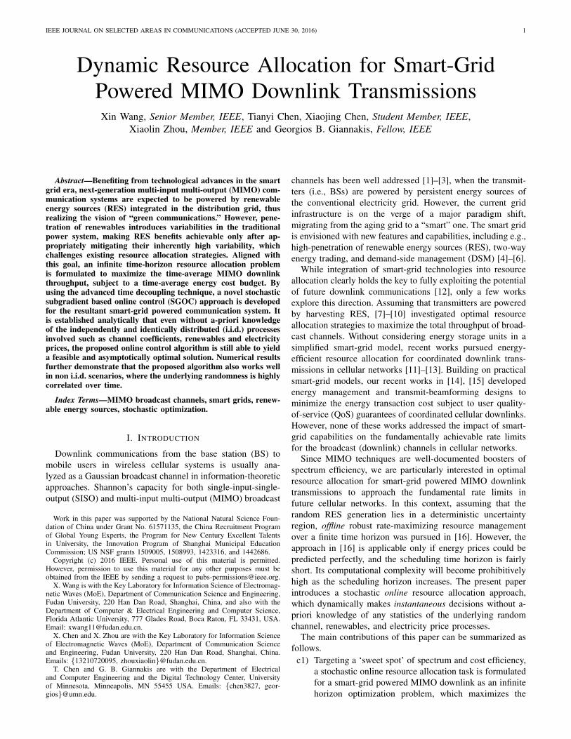
Consider a MIMO downlink where a BS with Nt antennascommunicates to K mobile users, each having Nr anten-nas; see Fig. 1. Powered by a smart microgrid, the BS isequipped with one or more energy harvesting devices (solarpanels and/or wind turbines), and can perform two-way energytrading with the main grid upon energy surplus or deficit inthe microgrid. In addition, with a goal of mitigating the highvariability of RES, an energy storage device (i.e., battery) isconsidered in the BS, so the BS does not have to consume orsell all the harvested energy on the spot, but can save it forlater use. A controller at the BS coordinates the energy tradingas well as the allocation of communication resources. Thiscentral entity can collect both the channel state information(CSI) through the feedback links from the users, as well asthe energy information (energy buying/selling prices) via thesmart meter installed at the BS.

A. MIMO Downlink ChannelsThe downlink from the BS to the users constitutes a broad-

cast channel (BC). Assume slot-based transmissions from the

BS to the users, and a quasi-static model for the wirelesschannels, where the channel coefficients remain invariant perslot but are allowed to vary across slots. This assumptionis reasonable when the length of the slot is selected to besmaller than the coherence time of the wireless channels.Suppose also a slowly time-varying setup so that the slot lengthis sufficiently large to accommodate the Shannon capacity-achieving encoding schemes. For convenience, the slot du-ration is normalized to unity; thus, the terms “energy” and“power” will be used interchangeably throughout the paper.Notice that our algorithm could also be extended to a two timescale scheduling approach, where the battery can be operatedin the slow scale, while the remaining decision variables inthe fast time scale [19].

Consider a (possibly infinite) scheduling horizon consistingof T slots, indexed by the set T := {0, . . . , T −1}. Per slot t,let Hk,t ∈ CNr×Nt denote the channel coefficient matrix fromthe BS to user k = 1, . . . ,K, and Ht := {H1,t, . . . ,HK,t}.For simplicity, we assume that Ht evolves according to anindependent and identically distributed (i.i.d.) random process.Note that the proposed algorithm in the sequel can be appliedwithout any modification to non-i.i.d. scenarios as well. Yet,performance guarantees in the non-i.i.d. case must be obtainedby applying the more sophisticated delayed Lyapunov drifttechniques in [20].

Let x(t) ∈ CNt×1 denote the transmitted vector signal,which is the sum of the signal independently transmitted toindividual users: x(t) =

∑Kk=1 xk(t). The received complex-

baseband signal at user k is then

yk(t) = Hk,tx(t) + zk(t) (1)

where zk(t) is additive complex-Gaussian noise with zeromean and covariance matrix I (the identity matrix of sizeNr).

The capacity of the MIMO BC can be achieved by dirtypaper coding (DPC) [21]. With DPC, users are sequentially en-coded such that each user sees no interference from previouslyencoded users. For the DPC codeword xk(t), the transmitcovariance matrix of user k is Γk,t := E[xk(t)x

†k(t)]. With

Px,t denoting the transmit-power budget at the BS per slot t,it holds that

∑Kk=1 tr(Γk,t) ≤ Px,t. The BC capacity region

per slot t is then given by

CBC(Px,t;Ht) = Co

(∪π

Rπ(Px,t;Ht)

)(2)

where Co(·) denotes the convex hull, the union is over allpermutations π of {1, 2, . . . ,K}, and

Rπ(Px,t;Ht) =∪

{Γk,t:∑K

k=1 tr(Γk,t)≤Px,t}

{(r1, . . . , rK) :

rπ(k) ≤ log

∣∣∣I +∑k

u=1 Hπ(u),tΓπ(u),tH†π(u),t

∣∣∣∣∣∣I +∑k−1

u=1 Hπ(u),tΓπ(u),tH†π(u),t

∣∣∣ , ∀k}.

Here rk denotes the achievable transmission rate for user k =1, . . . ,K, and | · | signifies the determinant operator.

IEEE JOURNAL ON SELECTED AREAS IN COMMUNICATIONS (ACCEPTED JUNE 30, 2016) 3

, + ,

Smart meter

Battery

Solar panel

Power grid

Central

controller

,

,

, + ,

Mobile users

BS

Grid-deployed

communication/

control links

Fig. 1. A smart-grid powered MIMO downlink system.

B. Smart Grid Operations

The BS can harvest RES and store the energy in the batteryfor future use. Let Et denote the (random) energy harvestedat the beginning of slot t at the BS, with Et ≤ Emax, ∀t.

Let C0 denote the initial energy, and Ct the state of charge(SoC) in the battery at the beginning of slot t. The batteryis assumed to have a finite capacity Cmax. Furthermore,for reliability purposes, it may be required to ensure that aminimum energy level Cmin is maintained at all times1; hence,we have Cmin ≤ Ct ≤ Cmax, ∀t ∈ T . Let Pb,t denotethe power delivered to or drawn from the battery at slot t,which amounts to either charging (Pb,t > 0) or discharging(Pb,t < 0). Hence, the stored energy obeys the dynamicequation

Ct+1 = Ct + Pb,t, ∀t. (3)

The amount of power (dis-)charged is also bounded by

Pminb ≤ Pb,t ≤ Pmax

b (4)

where Pminb < 0, and Pmax

b > 0.Per slot t, the total energy consumption Pg,t at the BS

includes the transmission-related power Px,t, and the rest thatis due to other components such as air conditioning, dataprocessor, and circuits, which can be collectively modeled asa constant power, Pc > 0 [13]; namely,

Pg,t = Pc + Px,t/ξ

where ξ > 0 denotes the power amplifier efficiency. Withoutloss of generality, we normalize the constant to ξ = 1; andfurther assume that Pg,t is bounded by Pmax

g .When the renewable harvested energy is insufficient, the

main grid can supply the needed Pg,t to the BS. With a two-way energy trading facility, the BS can also sell its surplus

1Battery will become unreliable with high depth-of-discharge (DoD) –percentage of maximum charge removed during a discharge cycle; hence,a minimum level Cmin is to avoid high DoD. Such a level could be alsorequired to support the BS operation in the event of a grid outage.

energy to the grid at a fair price in order to reduce operationalcosts. Given the required energy Pg,t, the harvested energyEt, and the battery charging energy Pb,t, the shortage energythat needs to be purchased from the grid for the BS is [Pg,t−Et+Pb,t]

+; or, the surplus energy (when the harvested energyis abundant) that can be sold to the grid is [Pg,t−Et+Pb,t]

−,where [a]+ := max{a, 0}, and [a]− := max{−a, 0}. Both theshortage and surplus energies are non-negative, and we haveat most one of them be positive at any time t.

Suppose that the energy can be purchased from the grid atprice αt, while the energy is sold to the grid at price βt per slott. Assume that the prices are bounded; i.e., αt ∈ [αmin, αmax],βt ∈ [βmin, βmax], ∀t. Note that we shall always set αt > βt,∀t, to avoid meaningless buy-and-sell activities of the BS forprofit. Per slot t, the transaction cost for the BS is given by

G(Pg,t, Pb,t) = αt[Pg,t − Et + Pb,t]+ − βt[Pg,t − Et + Pb,t]

−.(5)

Again for simplicity, we assume that the random vari-ables (Et, αt, βt) are generated according to an i.i.d. randomprocess, while generalization to non-i.i.d. scenarios can beaddressed using the techniques in [20].

III. DYNAMIC RESOURCE ALLOCATION ALGORITHM

Based on the models of Section II, we formulate andoptimize in this section, the allocation of resources forthe smart-grid powered broadcasting operation. Let wk de-note the priority weight for user k = 1, . . . ,K, Γt :={Γ1,t, . . . ,ΓK,t}, and Gmax the maximum the allowablepower cost at the BS. Over the scheduling horizon T ,the central controller at the BS determines the opti-mal transmit covariance matrices {Γt, ∀t}, transmit-power{Px,t, ∀t}, and battery charging energy {Pb,t, ∀t}, in or-der to maximize the average (weighted) total throughputlimT→∞

1T

∑Kk=1[wk

∑T−1t=0 (rBk (Γt))], subject to the aver-

age energy cost constraint limT→∞1T

∑T−1t=0 G(Pg,t, Pb,t) ≤

IEEE JOURNAL ON SELECTED AREAS IN COMMUNICATIONS (ACCEPTED JUNE 30, 2016) 4

Gmax. For notational brevity, we introduce the auxiliary vari-ables Pt := Pg,t + Pb,t, and formulate the problem as

max{Γt,Ct,Pt,Px,t,Pb,t}

limT→∞

1

T

K∑k=1

[wk

T−1∑t=0

(rBk (Γt))] (6a)

s. t. limT→∞

1

T

T−1∑t=0

G(Pt) ≤ Gmax (6b)

Pt = Px,t + Pb,t + Pc (6c)0 ≤ Pc + Px,t ≤ Pmax

g (6d)

Pminb ≤ Pb,t ≤ Pmax

b (6e)Ct+1 = Ct + Pb,t (6f)

Cmin ≤ Ct ≤ Cmax (6g)

rB(Γt) ∈ CBC(Px,t;Ht), ∀t. (6h)

A. Reformulation and Relaxation

With ψt := (αt − βt)/2 and ϕt := (αt + βt)/2, it followsreadily from (5) that

G(Pt) = ψt|Pt − Et|+ ϕt(Pt − Et).

Since αt > βt > 0, we have ϕt > ψt > 0 which clearlyimplies that G(Pt) is a convex function of Pt.

Now let us convexify the rate functions rBk (Γt). By theinformation-theoretic uplink-downlink duality [22], [23], theBC capacity region CBC(Px,t;Ht) can be alternatively charac-terized by the capacity regions of a set of “dual” multi-accesschannels (MACs). In the dual MAC, the received signal is

y(t) =K∑

k=1

H†k,txk(t) + z(t)

where xk(t) is the signal transmitted by user k, and z(t) isadditive complex-Gaussian with zero mean and covariance ma-trix I (the identity matrix of size Nt). Let Qk := E[xkx

†k] ≽ 0

denote the transmit covariance matrix of user k, and letp := [P1, . . . , PK ]⊤ collect the transmit-power budgets of allusers. For a given p, the MAC capacity region is

CMAC(p;H†t ) =

∪{Qk: tr(Qk)≤Pk, ∀k}

{(r1, . . . , rK) :

∑k∈S

rk ≤ log

∣∣∣∣∣I +∑k∈S

H†k,tQkHk,t

∣∣∣∣∣ , ∀S ⊆ {1, . . . ,K}}.

The uplink-downlink duality dictates that the BC capacityregion (2) equals the union of these MAC capacity regionscorresponding to all power vectors p satisfying

∑Kk=1 Pk ≤

Px,t; that is,

CBC(p;Ht) =∪

{p:∑K

k=1 Pk≤Px,t}

CMAC(p;H†t ). (7)

Using the definition

Rt(Px,t) := maxrB(Γt)∈CBC(Px,t;Ht)

K∑k=1

wkrBk (Γt)

[10, Lemma 1] has established the following result.

Lemma 1: The function Rt(Px,t) can be alternatively ob-tained by the optimal value of the problem:

maxQk≽0

K∑k=1

(wπ(k) − wπ(k+1)) log

∣∣∣∣∣I +

k∑u=1

H†π(u),tQπ(u)Hπ(u),t

∣∣∣∣∣s. t.

K∑k=1

tr(Qk) = Px,t

(8)where π is the permutation of user indices {1, . . . ,K} such thatwπ(1) ≥ · · · ≥ wπ(K), and wπ(K+1) = 0. In addition, Rt(Px,t) isa strictly concave and increasing function of Px,t.

Using Rt(Px,t) and expressing the variables {Pb,t} interms of {Pt, Px,t}, the optimal broadcasting problem canbe converted into the optimal sum-power allocation for anequivalent “point-to-point” link, as follows

max{Ct,Pt,Px,t}

limT→∞

1

T

T−1∑t=0

[Rt(Px,t)] (9a)

s. t. limT→∞

1

T

T−1∑t=0

G(Pt) ≤ Gmax (9b)

0 ≤ Px,t ≤ Pmaxg − Pc (9c)

Pminb ≤ Pt − Px,t − Pc ≤ Pmax

b (9d)Ct+1 = Ct + Pt − Px,t − Pc (9e)

Cmin ≤ Ct ≤ Cmax, ∀t. (9f)

The convexity of constraint (9b) has been clarified, andconstraints (9c)-(9f) are linear. As Rt(Px,t) is a concavefunction of Px,t per Lemma 1, problem (9) is a convexprogram. Note that here we implement a nested optimizationprocedure. Namely, we first solve (9) to find the optimal{C∗

t , P∗t , P

∗x,t, P

∗b,t}. Given P ∗

x,t per slot, we then solve theconvex optimization (8) to obtain the optimal “virtual” u-plink covariance matrices Qk(P

∗x,t), ∀k, and subsequently,

the desired downlink covariance matrices Γ∗k,t from Qk(P

∗x,t)

via uplink-downlink duality. Let R∗ denote the value of theobjective in (6) under an optimal control policy.

Although (9) becomes convex after judicious reformulation,it is still difficult to solve since we aim to maximize theaverage total throughput over an infinite time horizon. Inparticular, the battery energy level relations in (6f) couple theoptimization variables over the infinite time horizon, whichrenders the problem intractable for traditional solvers such asdynamic programming.

By recognizing that (6f) can be viewed as an energy queuerecursion, we next apply the time decoupling technique to turn(9) into a tractable form [17], [18]. For the queue of Ct, thearrival and departure are Pt and Px,t + Pc, respectively, perslot t. Over the infinite time horizon, the time-averaging ratesof arrival and departure are given by limT→∞

1T

∑T−1t=0 Pt and

Pc+limT→∞1T

∑T−1t=0 Px,t, respectively. Define the following

IEEE JOURNAL ON SELECTED AREAS IN COMMUNICATIONS (ACCEPTED JUNE 30, 2016) 5

expected values:

E[Rt(Px,t)] := limT→∞

1

T

T−1∑t=0

Rt(Px,t)

E[G(Pt)] := limT→∞

1

T

T−1∑t=0

G(Pt)

E[Pt] := limT→∞

1

T

T−1∑t=0

Pt, E[Px,t] := limT→∞

1

T

T−1∑t=0

Px,t

where the expectations are taken over all sources of ran-domness. These expectations exist due to the stationarity of{Ht, Et, αt, βt}.

Now simply remove the variables {Ct} and consider thefollowing problem

R̃∗ := max{Pt,Px,t}

E[Rt(Px,t)]

s. t. E[G(Pt)] ≤ Gmax, E[Pt] = Pc + E[Px,t]

(9c) − (9d).

(10)

It can be shown that (10) is a relaxed version of (9).Specifically, any feasible solution of (9) also satisfies theconstraints in (10). To see this, consider any policy thatsatisfies (9e) and (9f). Then summing equations in (9e) overall t ∈ T yields: CT −C0 =

∑T−1t=0 [Pt−Pc−Px,t]. Since both

CT and C0 are bounded due to (9f), dividing both sides byT and taking limits as T → ∞, yields E[Pt] = Pc + E[Px,t].It is then clear that any feasible policy for (9) is also feasiblefor (10). As a result, the optimal value of (10) is not less thanthat of (9); that is, R̃∗ ≥ R∗.

Note that the time coupling constraint (9e) has been relaxedin problem (10), which then becomes easier to solve. It canbe shown that the optimal solution to (10) can be achievedby a stationary control policy that chooses control actions{Pt, Px,t} every slot purely as a function (possibly random-ized) of the current {Ht, Et, αt, βt} [20]. We next develop astochastic dual subgradient solver for (10), which under properinitialization can provide an asymptotically optimal solution tothe original resource allocation problem (6).

B. Dual Subgradient Approach

Let Ft denote the set of {Pt, Px,t} satisfying constraints(9c)–(9d) per t, and λ := {λ1, λ2} collect the Lagrangemultipliers associated with the two average constraints. Withthe convenient notation Xt := {Pt, Px,t} and X := {Xt,∀t},the partial Lagrangian function of (10) is

L(X,λ) :=E[Rt(Px,t)]− λ1(E[G(Pt)]−Gmax)

− λ2(E[Pt]− Pc − E[Px,t]) (11)

while the Lagrange dual function is given by

D(λ) := max{Xt∈Ft}t

L(X,λ) (12)

and the dual problem of (10) is: minλ1≥0,λ2 D(λ).For the dual problem, we can resort to a standard subgradi-

ent method to obtain the optimal λ∗. This amounts to running

the iterations

λ1(j + 1) = [λ1(j)− µgλ1(j)]+

λ2(j + 1) = λ2(j)− µgλ2(j)(13)

where j is the iteration index, and µ > 0 is an appropriatestepsize. The subgradient g(j) := [gλ1(j), gλ2(j)] can be thenexpressed as

gλ1(j) = Gmax − E[G(Pt(j))]

gλ2(j) = Pc + E[Px,t(j)]− E[Pt(j)](14)

where Pt(j) and Px,t(j) are given by

{Pt(j), Px,t(j)} ∈ arg max{Pt,Px,t}∈Ft

[Rt(Px,t)

−λ1(j)G(Pt)− λ2(j)(Pt − Pc − Px,t)]. (15)

By the concavity of Rt(Px,t), convexity of G(Pt), and thenonnegativity of λ1(j), the objective function here is con-cave. Since F t is a convex set, the maximization prob-lem in (15) is a convex program. By Lemma 1, the prob-lem can be transformed into (16), which can be efficientlysolved by the Matlab CVX solver in polynomial time. With{Pt(λ(j)),Q

∗k(λ(j)), ∀k} denoting the optimal solution of

(16), one can subsequently determine Pt(j) = Pt(λ(j)), andPx,t(j) =

∑Kk=1 tr(Q∗

k(λ(j))).When a constant stepsize µ is adopted, the subgradient

iterations (13) are guaranteed to converge to a neighborhoodof the optimal λ∗ for the dual problem from any initialpoint λ(0). The size of the neighborhood is proportionalto the stepsize µ. In fact, if we adopt a sequence of non-summable diminishing stepsizes satisfying limj→∞ µ(j) = 0and

∑∞j=0 µ(j) = ∞, then the iterations (13) converge to the

exact λ∗ as j → ∞ [24]. Since (10) is convex, the dualitygap is zero, and convergence to λ∗ will also yield the optimalsolution {P ∗

t , P∗x,t,∀t} to the primal problem (10).

C. Online Control Algorithm

A challenge associated with the subgradient iterations (13)is computing E[Pt(j)], E[Px,t(j)], and E[G(Pt(j))] per iterate.This amounts to performing (high-dimensional) integrationover unknown joint distribution functions; or approximately,computing the corresponding time-averages over an infinitetime horizon. Clearly, such a requirement is impractical. Tobypass this impasse, we will rely on a stochastic subgradientapproach. Specifically, dropping E from (13), we propose thefollowing iteration

λ̂t+11 = [λ̂t1 − µ(Gmax −G(Pt(λ̂

t)))]+

λ̂t+12 = λ̂t2 − µ(Pc + Px,t(λ̂

t)− Pt(λ̂t))

(17)

where {λ̂t1, λ̂t2} are stochastic estimates of those in (13), andPt(λ̂

t), Px,t(λ̂t) are obtained by solving (15) with λ(j)

replaced by λ̂t.Note that t denotes both iteration and slot indices. In other

words, the update (17) is an online approximation algorithmbased on the instantaneous decisions {Pt(λ̂

t), Px,t(λ̂t)} per

slot t. This stochastic approach is made possible due tothe decoupling of optimization variables across time in (10).

IEEE JOURNAL ON SELECTED AREAS IN COMMUNICATIONS (ACCEPTED JUNE 30, 2016) 6

maxQk≽0,Pt≥0

K∑k=1

(wπ(k) − wπ(k+1)) log

∣∣∣∣∣I +

k∑u=1

H†π(u),tQπ(u)Hπ(u),t

∣∣∣∣∣+ λ2(j)

K∑k=1

tr(Qk)− λ2(j)Pt − λ1(j)G(Pt)

s. t. 0 ≤K∑

k=1

tr(Qk) ≤ Pmaxg − Pc, Pmin

b ≤ Pt −K∑

k=1

tr(Qk)− Pc ≤ Pmaxb

(16)

Convergence of online iterations (17) to the optimal λ∗ canbe established in different senses; see [20] and [25]–[27].

Based on the stochastic iterations (17), we will developnext a stochastic subgradient based online control (SGOC)algorithm for the original problem (6). The algorithm isimplemented at the BS as follows.

SGOC: Initialize with a proper λ̂0 := {λ̂01, λ̂02}. At everytime slot t, observe λ̂t,Ht, Et, αt, βt, and then do:

• Real-time energy management: Obtain {Pt(λ̂t),

Px,t(λ̂t)} by solving (15). Perform energy transaction

with the main grid; that is, buy the energy amount[Pt(λ̂

t)−Et]+ with price αt upon energy deficit, or, sell

the energy amount [Pt(λ̂t) − Et]

− with price βt uponenergy surplus. Charge (or discharge) the battery withthe amount Pb,t = Pt(λ̂

t)− Px,t(λ̂t)− Pc.

• Real-time broadcast schedule: Given the transmit-powerPx,t(λ̂

t) at the BS, solve the convex problem (8) to obtainthe optimal “dual” MAC transmit-covariance matrices{Qk(Px,t(λ̂

t)), ∀k}. With π being the permutation ofuser indices {1, . . . ,K} such that wπ(1) ≥ · · · ≥ wπ(K),define for k = 1, . . . ,K,

Ak := I +Hπ(k)

(k−1∑u=1

Γπ(u),t−1

)H†

π(k),

Bk := I +K∑

u=k+1

(H†

π(u)Qπ(u)(Px,t(λ̂t))Hπ(u)

).

Using Ak and Bk, find the optimal transmit covariancematrices: k = 1, . . . ,K,

Γπ(k),t = B− 1

2

k FkG†kA

12

kQπ(k)(Px,t(λ̂t))A

12

kGkF†kB

− 12

k

where the matrices Fk and Gk could be obtained by sin-gular value decomposition (SVD) of the effective channelHπ(k): B

− 12

k H†π(k)A

− 12

k = FkSG†k with a square and

diagonal matrix S [23].2 Perform MIMO broadcast withthe transmit covariance matrix Γk,t per user k.

• Lagrange multipliers updates: With Pt(λ̂t), Px,t(λ̂

t)available, update Lagrange multipliers λ̂t+1 via (17).

D. Performance Guarantees

Next, we will rigorously establish that the proposed algo-rithm asymptotically yields a feasible and optimal solution of(6) under proper initialization. To this end, we first establish

2Note that Γπ(1),t = B− 1

21 F1G

†1Qπ(1)(Px,t(λ̂t))G1F

†1B

− 12

1 , whichonly requires knowledge of Qk(Px,t(λ̂t)), ∀k. When calculating Γπ(k),t,k > 1, we need Ak whose calculation requires knowledge of previouslyobtained {Γπ(u),t}k−1

u=1. In such a sequential way, all Γk,t can be determined.

the asymptotic optimality of the proposed SGOC algorithm inthe following sense.Lemma 2: If {Ht, Et, αt, βt} are i.i.d. over slots, then thetime-averaging throughput under the proposed SGOC algo-rithm satisfies

limT→∞

1

T

T−1∑t=0

E[Rt(Px,t(λ̂t))] ≥ R∗ − µM

where the constant is given by

M :=1

2

[(max{Pmax

b ,−Pminb })2 + (Gmax)2+

(max{αmax(Pmaxg + Pmax

b ), βmax(Emax − Pminb )})2

] (18)

and R∗ is the optimal value of (9), or, equivalently, (6), underany feasible control algorithm, even if that relies on knowingfuture random realizations.

Proof: See Appendix A.Lemma 2 asserts that the proposed SGOC algorithm con-

verges to a region with optimality gap smaller than µM , whichvanishes as the stepsize µ→ 0. The proof mimics the lines ofthe Lyapunov optimization technique in e.g., [20]. Yet, slightlydifferent from [20], here the Lagrange dual theory is utilizedto simplify the arguments.

We have shown that the SGOC iteration can achieve a near-optimal objective value for (9). However, since the proposedalgorithm is based on a solver for the relaxed (10), it isnot guaranteed that the resultant dynamic control policy isa feasible one for (9). In the sequel, we will establish that theSGOC in fact can yield a feasible policy for (9), when it isproperly initialized.

Since Rt(Px,t) is strictly concave and increasing per Lem-ma 1, it has left and right derivatives at any Px,t, and the leftderivative is no less than the right one. Let R′

t(Px,t) be theleft (or right) derivative of Rt(Px,t). Clearly, R′

t(Px,t) ≥ 0is strictly decreasing in Px,t. Let R′(0) := max{R′

t(0), ∀t},and assume R′(0) < ∞ (this holds when Hk,t, ∀k, t, havebounded maximum eigenvalues). We can show that:Lemma 3: The BS transmit-powers Px,t under the SGOCalgorithm satisfy: Px,t(λ̂

t) = 0, if λ̂t1 >R′

t(0)βt

. In addition,the battery (dis-)charging amounts Pb,t under the SGOC obey:i) Pb,t(λ̂

t) = Pminb , if λ̂t2 > −λ̂t1βt; and ii) Pb,t(λ̂

t) = Pmaxb ,

if λ̂t2 < −λ̂t1αt.Proof: See Appendix B.

Lemma 3 reveals partial characteristics of the dynamic S-GOC policy. Such a structure can be justified by the economicinterpretation of the Lagrange multipliers. Specifically, λ̂t1 andλ̂t2 can be viewed as the stochastic instantaneous power andcharging prices, respectively. When the power price λ̂t1 is high,zero transmit-power is adopted at the BS, i.e., Px,t(λ̂

t) = 0.

IEEE JOURNAL ON SELECTED AREAS IN COMMUNICATIONS (ACCEPTED JUNE 30, 2016) 7

For high charging prices λ̂t2 > −λ̂t1βt, the SGOC dictatesthe full discharge Pb,t(λ̂

t) = Pminb . Conversely, the battery

units can afford full charge if the charging price is low; i.e.,λ̂t2 < −λ̂t1αt. Note that here, whether the charging price λ̂t2is high or low, depends also on the power price λ̂t1.

Based on the structure revealed by Lemma 3, we can firstestablish the following lemma.Lemma 4: If αmax(Pc + Pmax

b ) ≤ Gmax, then the SGOCguarantees: 0 ≤ λ̂t1 ≤ R′(0)

βmin + max{0, µ(αmax(Pmaxg +

Pmaxb )−Gmax)}, ∀t.

Proof: See Appendix C.Note that αmax(Pc+P

maxb ) ≤ Gmax is in fact a mild condi-

tion, which implies that the BS has a (minimum) power budgetto support its normal operation and full battery charge at anytime. Use short-hand notation δλ1 := max{0, αmax(Pmax

g +Pmaxb )−Gmax}. Leveraging the bounds in Lemma 4 and the

structure in Lemma 3, we can subsequently establish that:Lemma 5: If the stepsize satisfies µ ≥ µ, where

µ :=αmaxR′(0)

βmin(Cmax − Cmin + Pminb − Pmax

b − δλ1)(19)

then the SGOC guarantees the Lagrange multiplierλ̂t2 ∈ [−αmax(R

′(0)βmin + µδλ1) + µPmin

b , µCmax − µCmin −αmax(R

′(0)βmin + µδλ1) + µPmin

b ], ∀t.Proof: See Appendix D.

Consider now the linear mapping

Ct =λ̂t2µ

+αmaxR′(0)

µβmin+ αmaxδλ1 + Cmin − Pmin

b . (20)

It can be readily inferred from Lemma 5 that Cmin ≤Ct ≤ Cmax holds, ∀t; i.e, (9f) is always satisfied under theSGOC. With the battery (dis-)charging dynamics (9e) naturallyperformed, it follows that the proposed SGOC scheme yieldsa feasible dynamic control policy for the problem (9).Remark 1: The Lagrange multiplier λ̂t2 in (20) can be re-garded as a scaled version of the “perturbed” energy queue-size Ct; that is, λ̂t2 equals Ct after subtracting a constant(αmax/µβmin)R′(0) + αmaxδλ1 + Cmin − Pmin

b , and thenmultiplying by a scalar µ. Hence, λ̂t2 can be treated as a“virtual” queue, and likewise for λ̂t1. Different from [15] and[17], where such “virtual queues” evolve independently, theevolution of λ̂t2 in (17) clearly depends on the value of λ̂t1,and vice-versa; e.g., {Pt(λ̂

t), Px,t(λ̂t)} are actually functions

of λ̂t := {λ̂t1, λ̂t2}, and Pb,t(λ̂t) is characterized by the joint

relationship among λ̂t1, λ̂t2, αt, βt. This is markedly different

from a simple threshold-based (dis-)charging profile in [15,Lemma 2] and [17, Lemma 2]. In this sense, the coupling ofthe “virtual queues” complicates matters, and the performanceanalysis framework in [15], [17] is generalized here to includeconditions that ensure feasibility of the proposed algorithm.Specifically, by exploiting the revealed characteristics of ourSGOC policy, we first establish bounds for λ̂t1 in Lemma 4.Capitalizing on the specific coupling of the two “queues,” wefurther establish a lower bound on the stepsize µ to ensure thebounds for λ̂t2 in Lemma 5.

Based on Lemmas 2, 4 and 5, we arrive at the main result.

TABLE IPARAMETERS CONFIGURATION.

Gmax Pmaxg Pmin

b Pmaxb Cmin Cmax C0

15 50 -5 5 0 50 0

Theorem 1: If we set λ̂01 ∈ [0, R′(0)

βmin +µδλ1 ], and λ̂02 = µC0−µCmin + µPmin

b − αmax(R′(0)

βmin + µδλ1), and select a stepsizeµ ≥ µ, then the proposed SGOC yields a feasible dynamiccontrol scheme for (9), which is asymptotically optimal in thesense that

limT→∞

1

T

T−1∑t=0

E[Rt(Px,t(λ̂t))] ≥ R∗ − µM

where M and µ are given by (18) and (19), respectively.Remark 2: Choosing µ = µ, the minimum optimality gap(regret) between the SGOC, and the offline scheduling isclearly given by µM . The asymptotically optimal solution canbe attained if the power purchase prices αt are very small, or,the battery capacities Cmax are large enough, so that µ → 0.This makes sense intuitively because when the BS batteryhas large capacity, the upper bound in (9f) is loose. In thiscase, with proper initialization, the SGOC using any µ will befeasible for (9), or, (6).

IV. NUMERICAL RESULTS

In this section, simulations are presented to evaluate ourproposed dynamic approach, and justify the analytical claimsof Section III.

The considered MIMO downlink has a BS with Nt = 2antennas, communicating to K = 10 mobile users equippedwith Nr = 2 antennas each. The system bandwidth is 1 MHz,and each element in channel coefficient matrix Hk,t, ∀k, t,is a zero-mean complex-Gaussian random variable with unitvariance. The default parameters are listed in Table I. Theenergy purchase price αt is uniformly distributed within [0.1,1] and the selling price is set as β = rα with r = 0.9.Samples of the harvested energy Et are generated from aWeibull distributed wind speed using the wind-speed-to-wind-power mapping. An autoregressive model is adopted to capturethe possible spatio-temporal correlations as in [28]. Althoughall the random quantities are assumed i.i.d. in our performanceanalysis, here the renewable generations are actually generatedfrom the non i.i.d. process in order to better simulate the real-world traces. Finally, the stepsize is chosen as µ = µ [cf.Theorem 1] by default.

The proposed SGOC algorithm is compared with twobaseline schemes to benchmark its performance. ALG 1 is a“greedy” scheme that maximizes the instantaneous throughputper time slot without leveraging the battery. Specifically, theinstantaneous decisions {Pt, Px,t} are obtained by solving theconvex problem (9) per slot t without (dis-)charging, i.e.,Pb,t = 0. The instantaneous throughput maximization and lackof a storage device make ALG 1 myopic, and vulnerable tofuture high purchase prices. ALG 2 is similar to the proposedone in the sense that it uses the stochastic dual subgradientto iteratively approximate the primal solution. Yet, neither

IEEE JOURNAL ON SELECTED AREAS IN COMMUNICATIONS (ACCEPTED JUNE 30, 2016) 8

0 50 100 150 200 250 3005.5

6

6.5

7

7.5

8

8.5

9

9.5

Time Slot

Ave

rage

Thr

ough

put (

Mbp

s)

Proposed AlgorithmALG 1ALG 2

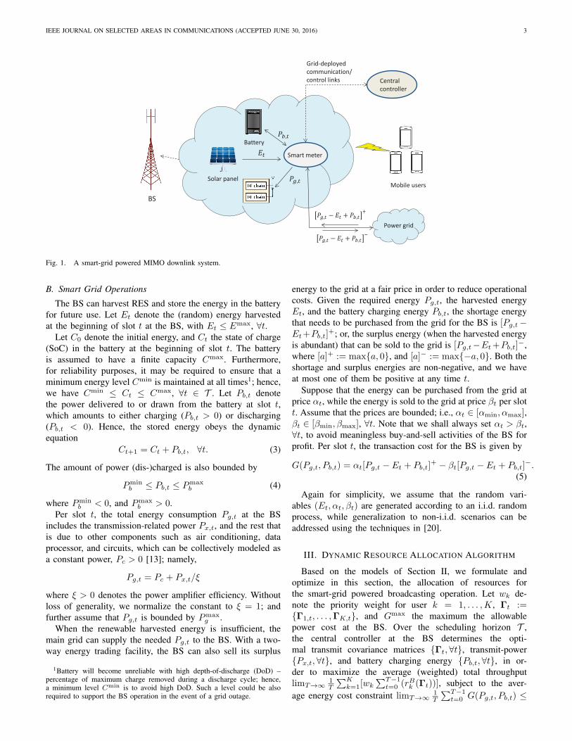
Fig. 2. Comparison of average throughput.

0 50 100 150 200 250 3004

5

6

7

8

9

10

Time Slot

Ave

rage

Thr

ough

put (

Mbp

s)

µ= µ

µ= 0.1µ

µ= 0.01µ

Upper Bound

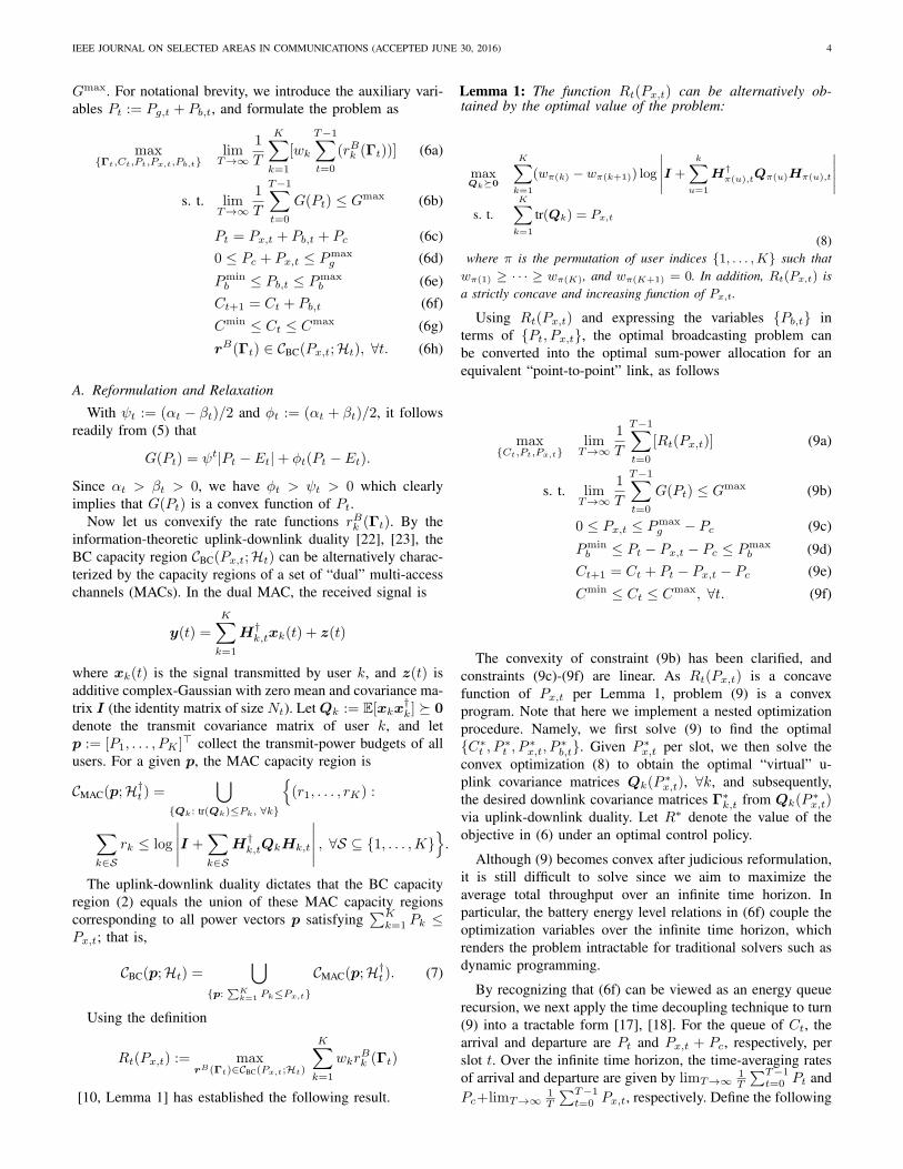
Fig. 3. Average throughput versus stepsize µ.

renewable energy nor battery is taken into account, and onlyone-way trading mechanism is adopted between the BS andgrid market implying that all consumed energy are boughtfrom grid with no energy sold in the energy surplus case.

Fig. 2 compares the average throughputs of the proposedalgorithm and ALGs 1-2 over time slots. It is observed thatwithin 300 time slots, the proposed approach converges tothe largest throughput, while ALGs 1-2 incur about 3.0%and 13.3% smaller throughputs. Intuitively speaking, this isbecause the proposed algorithm intelligently leverages therenewable energy and energy storage device to hedge againstfuture losses, which cannot be fully exploited by ALGs 1-2.

Fig. 3 validates the impact of the stepsize µ on the averagethroughput of the proposed algorithm. The average throughputis compared under different µ = {0.01µ, 0.1µ, µ}. The dottedupper bound is obtained in the case where Px,t = Pmax

g −Pc

for all time slots t without considering the maximum budgetGmax. It is shown that the proposed algorithm always con-verges to a value lower than the upper bound with differentstepsize µ. However, it approaches the upper bound with a

4 6 8 10 12 14 16 18 200

10

20

30

40

50

60

70

80

90

100

Time Slot

Ct (

kWh)

µ= µ

µ= 0.1µ

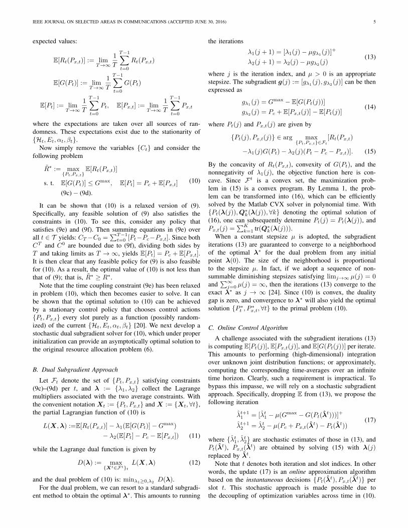
Fig. 4. The battery state-of-charge Ct versus stepsize µ, where Pmaxg =

10 kWh.

0 2 4 6 8 10 12−3

−2

−1

0

Time Slot

Pric

es

1 2 3 4 5 6 7 8 9 10 11−5

0

5

Time Slot

P b,t (

kWh)

−λ̂t1βt

−λ̂t1αt

ˆλt2

Fig. 5. SGOC based schedule of battery power Pb,t, where Pmaxg = 10 k-

Wh.

smaller stepsize. Specifically, when µ = 0.01µ, the proposedalgorithm obtains an average throughput only 3.2% lower thanthe upper bound, which is consistent with Lemma 2 in a waythat the optimality gap is proportional to the stepsize µ.

However, as stated in Lemma 5, the value of stepsizeµ can significantly affect feasibility of the proposed onlinescheme. Fig. 4 illustrates the evolution of battery SoC Ct withdifferent µ = {0.1µ, µ}. It reveals that Ct is always within theprescribed bounds (i.e., Cmin ≤ Ct ≤ Cmax) when µ = µ.In contrast, if a smaller stepsize µ = 0.1µ is chosen, Ct willviolate its physical upper bound frequently.

In Fig. 5, −λ̂t1αt, −λ̂t1βt, λ̂t2 as well as Pb,t are jointlydepicted to demonstrate the (dis-)charging rules revealed byLemma 3. It can be seen that the SGOC dictates the full dis-charge Pb,t = Pmin

b when λ̂t2 > −λ̂t1βt at t = 2, 5, 7, 10, whilethe battery is fully charged Pb,t = Pmax

b when λ̂t2 < −λ̂t1αt

at t = 1, 3, 6, 8, 11. In addition, when λ̂t2 ∈ [−λ̂t1αt,−λ̂t1βt]at t = 4, 9, Pb,t can only been obtained by solving (16)numerically. Note that the insightful online policy are also

IEEE JOURNAL ON SELECTED AREAS IN COMMUNICATIONS (ACCEPTED JUNE 30, 2016) 9

0 5 10 15 20 250

1

2

3

4

5

6

7

8

Time Slot

P x,t (

kWh)

αt

Fig. 6. SGOC based schedule of transmission-related power Px,t.

10 15 20 25 30 35 40

7

7.5

8

8.5

9

9.5

Gmax

Ave

rage

Thr

ough

put (

Mbp

s)

Proposed AlgorithmALG 1ALG 2Upper Bound

Pmaxg =50 kWh

Pmaxg =30 kWh

Fig. 7. Average throughput versus Gmax.

applicable for the slots after t = 11, and it can be furtherobserved that the Lagrange multiplier λ̂t2 is in fact an affinemapping of the real-time battery SoC Ct [cf. 21].

Fig. 6 depicts the optimal power schedule Px,t of the pro-posed SGOC over time, and the fluctuation of energy purchaseprices αt is also plotted to illustrate the resultant online policy.It can be clearly observed that the power consumption highlydepends on the instantaneous energy purchase price αt. Specif-ically, the proposed scheme tends to consume more powerwhen αt is lower (e.g., t = 2, 12, 24), and tends to consumeless power when αt is higher (e.g., t = 3, 14, 15). In otherwords, the proposed method allows purchasing more energyfrom the smart-grid when energy purchase price αt is lower foreconomic concern. Fig. 6 shows that the transmission-relatedpower Px,t follows the opposite trend to the price fluctuation.

The average throughputs of the SGOC and ALGs 1-2 arecompared with respect to the growth of Gmax in Fig. 7. Clear-ly, the throughputs of all three algorithms increase as Gmax orPmaxg increases since larger energy cost or looser maximum

energy consumption limit will allow more energy purchasesfrom the smart grid and larger energy consumption, leading to

the increase of average throughputs. In both cases, we observethat the proposed algorithm performs better than ALGs 1-2. For instance, when Gmax = 10 and Pmax

g = 50 kWh,the proposed scheme has 5.0% and 24.3% gains in averagethroughput over ALGs 1 and 2, respectively. Besides, it turnsout that the average throughput of the SGOC approaches theupper bounds when Gmax is large or Pmax

g is small. Intuitivelyspeaking, with a limited Pg,t, a large Gmax becomes redundantso that the SGOC could always allocate maximal transmissionpower to increase throughput. We can see that the proposedalgorithm converges faster than ALGs 1-2 with a given Pmax

g ,which also means it expects a smaller budget in order to“saturate.”

V. CONCLUSIONS

In this paper, real-time resource allocation was developedfor smart-grid powered MIMO downlink transmissions. Tak-ing into account the time variations of channels, harvestedrenewables and electricity prices, a stochastic optimizationproblem was formulated to maximize the expected through-put while satisfying the energy cost constraints. Relying onthe stochastic subgradient method, an online algorithm wasdeveloped to obtain feasible decisions ‘on-the-fly’ by relaxingthe time-coupling storage and budget dynamics. It was proventhat the novel approach yields feasible and asymptoticallyoptimal resource schedules without knowing any statisticsof the underlying stochastic processes. Simulations furthercorroborated the merits of the proposed scheme in non i.i.d.cases, where the underlying randomness is highly correlatedover time. In the guidance of present work, interesting futureworks include modeling more practical storage units withenergy leakage, considering the power network structures, andpursuing the two-timescale energy management and wirelessresource allocation mechanism.

APPENDIX

A. Proof of Lemma 2

From recursions (13), we deduce

(λ̂t+12 )2 ≤ [λ̂t2 − µ(Pc + Px,t(λ̂

t)− Pt(λ̂t)]2

= (λ̂t2)2 − 2µλ̂t2[Pc + Px,t(λ̂

t)− Pt(λ̂t)]

+ µ2[Pc + Px,t(λ̂t)− Pt(λ̂

t)]2

≤ (λ̂t2)2 − 2µλ̂t2[Pc + Px,t(λ̂

t)− Pt(λ̂t)]

+ µ2(max{Pmaxb,i ,−Pmin

b,i })2

where the last inequality holds due to (9d). Similarly, it followsthat

(λ̂t+11 )2 ≤ (λ̂t1)

2 − 2µλ̂t1[Gmax −G(Pt(λ̂

t)] + µ2[(Gmax)2

+ (max{αmax(Pmaxg + Pmax

b ), βmax(Emax − Pminb )})2].

Considering now the Lyapunov function V (λ̂t) :=12 [(λ̂

t1)

2 + (λ̂t2)2], it readily follows that

−△V (λ̂t) := −V (λ̂t+1) + V (λ̂t)

≥ µλ̂t2[Pc + Px,t(λ̂t)− Pt(λ̂

t)]

+ µλ̂t1[Gmax −G(Pt(λ̂

t)]− µ2M.

IEEE JOURNAL ON SELECTED AREAS IN COMMUNICATIONS (ACCEPTED JUNE 30, 2016) 10

Taking expectations and adding µE[Rt(Px,t(λ̂t))] to both

sides, we arrive at

E[−△V (λ̂t)] + µE[Rt(Px,t(λ̂t))]

≥ µ(E[Rt(Px,t(λ̂

t))] + λ̂t2[Pc + Px,t(λ̂t)− Pt(λ̂

t)]

+ λ̂t1[Gmax −G(Pt(λ̂

t)])− µ2M

= µL(X(λ̂t), λ̂t)− µ2M

= µD(λ̂t)− µ2M

≥ µR̃∗ − µ2M

where we used the definition of L(X,λ) in (11); X(λ̂t)denotes the optimal primal variable set given by (15) forλ = λ̂t (hence, L(X(λ̂t), λ̂t) = D(λ̂t)); R̃∗ denotes theoptimal value for problem (10); and the last inequality is dueto the weak duality: D(λ) ≥ R̃∗, ∀λ.

Summing over all t, we then have

T−1∑t=0

E[−△V (λ̂t)] + µ

T−1∑t=0

E[Rt(Px,t(λ̂t))]

= −E[V (λ̂T )] + V (λ̂0) + µT−1∑t=0

E[Rt(Px,t(λ̂t))]

≥ T (µR̃∗ − µ2M)

which leads to

1

T

T−1∑t=0

E[Rt(Px,t(λ̂t))] ≥ R̃∗ − µM − V (λ̂0)

µT

≥ R∗ − µM − V (λ̂0)

µT.

The lemma follows by taking the limit T → ∞.

B. Proof of Lemma 3

Recall that Pb,t = Pt−Pc−Px,t. Given λ̂t, we can rewritethe maximization problem in (15) in terms of {Px,t, Pb,t} as

maxPx,t,Pb,t

Rt(Px,t)− λ̂t1G(Pb,t + Pc + Px,t)− λ̂t2Pb,t

s. t. 0 ≤ Px,t ≤ Pmaxg − Pc, Pmin

b ≤ Pb,t ≤ Pmaxb .

(21)

Consider the following two cases [cf. (5)]i) If Pb,t + Pc + Px,t ≥ Et, then G(Pb,t + Pc + Px,t) =αt(Pb,t + Pc + Px,t − Et). The problem (21) can bedecomposed into two subproblems, namely

max0≤Px,t≤Pmax

g −Pc

Rt(Px,t)− λ̂t1αtPx,t

maxPmin

b ≤Pb,t≤Pmaxb

−(λ̂t1αt + λ̂t2)Pb,t.

Let R′t−1 denote the inverse function of R′

t. It is easy tosee that we must have

Px,t(λ̂t) = max{0,min{Pmax

g − Pc, R′t−1

(λ̂t1αt)}}.

Pb,t(λ̂t) =

{Pminb , if λ̂t1αt + λ̂t2 > 0

Pmaxb , if λ̂t1αt + λ̂t2 < 0.

ii) If Pb,t + Pc + Px,t < Et, then G(Pb,t + Pc + Px,t) =βt(Pb,t + Pc + Px,t − Et); and we similarly arrive at

Px,t(λ̂t) = max{0,min{Pmax

g − Pc, R′t−1

(λ̂t1βt)}}.

Pb,t(λ̂t) =

{Pminb , if λ̂t1βt + λ̂t2 > 0

Pmaxb , if λ̂t1βt + λ̂t2 < 0.

Combining cases i) and ii), we deduce that per slot t, if λ̂t1 >max{R′

t(0)/αt, R′t(0)/βt} = R′

t(0)/βt, then Px,t(λ̂t) = 0.

Similarly, if λ̂t2 > max{−λ̂t1αt,−λ̂t1βt} = −λ̂t1βt, thenPb,t(λ̂

t) = Pminb ; and if λ̂t2 < min{−λ̂t1αt,−λ̂t1βt} =

−λ̂t1αt, then Pb,t(λ̂t) = Pmax

b .

C. Proof of Lemma 4

Due to the projection operation, it is clear λ̂t1 ≥ 0. Wenext establish the upper bound for λ̂t1 by induction. First, setλ̂01 ≤ R′(0)

βmin +max{0, µ(αmax(Pmaxg + Pmax

b )−Gmax)}, andsuppose that this holds for all λ̂t1 at slot t. We show that thebound holds for λ̂t+1

1 as well, in the following two cases.

c1) If λ̂t1 ∈ [0, R′(0)

βmin ], we have λ̂t+11 = [λ̂t1 + µ(G(Pt(λ̂

t))−Gmax)]+ ≤ R′(0)

βmin + max{0, µ(αmax(Pmaxg + Pmax

b ) −Gmax)}, since G(Pt(λ̂

t)) ≤ αmax(Pmaxg +Pmax

b ) due toPt(λ̂

t) ≤ Pmaxg +Pmax

b by the constraints (9c)–(9d), andG(Pt) is increasing in Pt.

c2) If αmax(Pmaxg + Pmax

b ) − Gmax ≥ 0 and λ̂t1 ∈(R

′(0)βmin ,

R′(0)βmin + µ(αmax(Pmax

g + Pmaxb ) − Gmax)], then

we must have Px,t(λ̂t) = 0 by Lemma 2; thus,

Pt(λ̂t) ≤ Pc + Pmax

b . It follows that λ̂t+11 = [λ̂t1 +

µ(G(Pt(λ̂t)) − Gmax)]+ ≤ [R

′(0)βmin + µ(αmax(Pmax

g +

Pmaxb ) − Gmax) + µ(αmax(Pc + Pmax

b ) − Gmax)]+ ≤R′(0)βmin +µ(αmax(Pmax

g +Pmaxb )−Gmax), since αmax(Pc+

Pmaxb ) ≤ Gmax.

D. Proof of Lemma 5

The proof again proceeds by induction. First, setλ̂02 ∈ [−αmax(R

′(0)βmin + µδλ1) + µPmin

b , µCmax − µCmin −αmax(R

′(0)βmin + µδλ1) + µPmin

b ], and suppose that this holdsfor all λ̂t2 at slot t. Define short-hand notation λmax

1 :=R′(0)βmin + µδλ1 . We next show that the bounds hold for λ̂t+1

2

as well, in subsequent instances.c1) If λ̂t2 ∈ (0, µCmax − µCmin − αmaxλmax

1 + µPminb ], it

is clear that λ̂t2 > 0 > max{−λ̂t1βt, ∀t}. It then followsfrom Lemma 3 that λ̂t+1

2 = λ̂t2+µPminb ∈ [−αmaxλmax

1 +µPmin

b , µCmax − µCmin − αmaxλmax1 + µPmin

b ], sincePminb < 0.

c2) If λ̂t2 ∈ [−αmaxλmax1 , 0], then λ̂t+1

2 = λ̂t2 +µP t

b (λ̂t) ∈ [λ̂t2+µP

minb , λ̂t2+µP

maxb ] ⊆ [−αmaxλmax

1 +µPmin

b , µPmaxb ] ⊆ [−αmaxλmax

1 + µPminb , µCmax −

µCmin − αmaxλmax1 + µPmin

b ], where the upper boundholds when µ ≥ µ ≥ αmaxλmax

1

Cmax−Cmin+Pminb −Pmax

b

.

c3) If λ̂t2 ∈ [−αmaxλmax1 + µPmin

b ,−αmaxλmax1 ), it holds

that λ̂t2 < −αmaxλmax1 < min{−λ̂t1αt, ∀t}. By Lemma

3, we have λ̂t+12 = λ̂t2 + µPmax

b ∈ [−αmaxλmax1 +

IEEE JOURNAL ON SELECTED AREAS IN COMMUNICATIONS (ACCEPTED JUNE 30, 2016) 11

µPminb +Pmax

b ,−αmaxλmax1 +Pmax

b ) ⊆ (−αmaxλmax1 +

µPminb , µCmax − µCmin − αmaxλmax

1 + µPminb ), where

the last step follows from the facts Pmaxb > 0, and

−αmaxλmax1 + Pmax

b ≤ Pmaxb ≤ µCmax − µCmin −

αmaxλmax1 + µPmin

b when µ ≥ µ.

REFERENCES

[1] T. M. Cover and J. A. Thomas, Elements of Information Theory, 2ndEd., John Wiley & Sons, Inc., 2006.

[2] L. Li and A. J. Goldsmith, “Capacity and optimal resource allocationfor fading broadcast channels – Part I: Ergodic capacity,” IEEE Trans.Inf. Theory, vol. 47, no.3, pp. 1083–1102, Mar. 2001.

[3] H. Weingarten, Y. Steinberg, and S. Shamai, “The capacity region ofthe Gaussian multiple-input multiple-output broadcast channel,” IEEETrans. Inf. Theory, vol. 52, no. 9, pp. 3936–3964, Sep. 2006.

[4] A. Tolli, H. Pennanen, and P. Komulainen, “Decentralized minimumpower multi-cell beamforming with limited backhaul signaling,” IEEETrans. Wireless Commun., vol. 10, no. 2, pp. 570–580, Feb. 2011.

[5] Y. Zhang, N. Gatsis, and G. B. Giannakis, “Robust energy managementfor microgrids with high-penetration renewables,” IEEE Trans. Sustain.Energy, vol. 4, no. 4, pp. 944–953, Oct. 2013.

[6] G. B. Giannakis, V. Kekatos, N. Gatsis, S. Kim, H. Zhu, and B.Wollenberg, “Monitoring and optimization for power grids: A signalprocessing perspective,” IEEE Signal Process. Mag., vol. 30, no. 5, pp.107–128, Sept. 2013.

[7] M. Antepli, E. Uysal-Biyikoglu, and H. Erkal, “Optimal packet schedul-ing on an energy harvesting broadcast link,” IEEE J. Sel. Areas Com-mun., vol. 29, no. 8, pp. 1721–1731, Sep. 2011.

[8] J. Yang, O. Ozel, and S. Ulukus, “Broadcasting with an energy harvest-ing rechargeable transmitter,” IEEE Trans. Wireless Commun., vol. 11,no. 2, pp. 571–583, Feb. 2012.

[9] O. Ozel, J. Ying, and S. Ulukus, “Optimal broadcast scheduling for anenergy harvesting rechargeable transmitter with a finite capacity battery,”IEEE Trans. Wireless Commun., vol. 11, no. 6, pp. 2193–2203, Jun.2012.

[10] X. Wang, Z. Nan, and T. Chen, “Optimal MIMO broadcasting for energyharvesting transmitter with non-ideal circuit power consumption,” IEEETrans. Wireless Commun., vol. 14, no. 5, pp. 2500–2512, May 2015.

[11] S. Bu, F. Yu, Y. Cai, and X. Liu, “When the smart grid meets energy-efficient communications: Green wireless cellular networks powered bythe smart grid,” IEEE Trans. Wireless Commun., vol. 11, no. 8, pp.3014–3024, Aug. 2012.

[12] J. Xu, Y. Guo, and R. Zhang, “CoMP meets energy harvesting: A newcommunication and energy cooperation paradigm,” IEEE Trans. Veh.Technol., vol. 64, no. 6, pp. 2476–2488, Jun. 2015.

[13] J. Xu and R. Zhang, “Cooperative energy trading in CoMP systems pow-ered by smart grids,” IEEE Trans. Veh. Technol., Apr. 2015 (accepted),[Online]. Available: http://arxiv.org/pdf/1403.5735v2.pdf.

[14] X. Wang, Y. Zhang, G. B. Giannakis, and S. Hu, “Robust smart-grid powered cooperative multipoint systems,” IEEE Trans. WirelessCommun., vol. 14, no. 11, pp. 6188-6199, Nov. 2015.

[15] X. Wang, Y. Zhang, T. Chen, and G. B. Giannakis, “Dynamic energymanagement for smart-grid powered coordinated multipoint systems,”IEEE J. Sel. Areas Commun., to appear 2016.

[16] S. Hu, X. Wang, Y. Zhang, and G. B. Giannakis, “Optimal resourceallocation for smart-grid powered MIMO broadcast channels,” in Proc.WCSP, Nanjing, P.R. China, Oct. 2015.

[17] R. Urgaonkar, B. Urgaonkar, M. Neely, and A. Sivasubramaniam,“Optimal power cost management using stored energy in data centers,”in Proc. ACM SIGMETRICS, pp. 221–232, San Jose, CA, June 2011.

[18] S. Lakshminaryana, H. V. Poor, and T. Quek, “Cooperation and storagetrade-offs in power grids with renewable energy resources,” IEEE J. Sel.Areas Commun., vol. 32, no. 7, pp. 1–12, Jul. 2014.

[19] Y. Yao, L. Huang, A. Sharma, L. Golubchik, and M. Neely, “Datacenters power reduction: A two time scale approach for delay tolerantworkloads,” in Proc. INFOCOM, pp. 1431–1439, 2012.

[20] L. Georgiadis, M. Neely, and L. Tassiulas, “Resource allocation andcross-layer control in wireless networks,” Found. and Trends in Net-working, vol. 1, pp. 1–144, 2006.

[21] U. Erez, and S. ten Brink, “A close-to-capacity dirty paper codingscheme,” IEEE Trans. Inf. Theory, vol. 51, no. 10, pp. 3417–3432, May2004.

[22] N. Jindal, S. Vishwanath, and A. J. Goldsmith, “On the duality ofGaussian multiple-access and broadcast channels,” IEEE Trans. Inf.Theory, vol. 50, no. 5, pp. 768–783, Oct. 2005.

[23] S. Vishwanath, N. Jindal, and A. Goldsmith, “Duality, achievable rates,and sum-rate capacity of Gaussian MIMO broadcast channels,” IEEETrans. Inf. Theory, vol. 49, no. 10, pp. 2658–2668, Oct. 2003.

[24] D. P. Bertsekas, Convex Optimization Theory, Athena Scientific, 2009.[25] A. Stolyar, “Maximizing queueing network utility subject to stability:

Greedy primal-dual algorithm,” Queueing Syst., vol. 50, pp. 401–457,2005.

[26] A. Eryilmaz and R. Srikant, “Fair resource allocation in wirelessnetworks using queue-length-based scheduling and congestion control,”IEEE Trans. Netw., vol. 15, no. 6, pp. 1333–1344, Dec. 2007.

[27] X. Wang, G. B. Giannakis, and A. G. Marques, “A unified approachto QoS-guaranteed scheduling for channel-adaptive wireless networks,”Proc. IEEE, vol. 95, no. 12, pp. 2410–2431, Dec. 2007.

[28] Y. Zhang, N. Gatsis, and G. B. Giannakis, “Risk-constrained energymanagement with multiple wind farms,” in Proc. of 4th IEEE-PES onInnovative Smart Grid Tech., Washington, D.C., Feb. 2013.

Xin Wang (SM’09) received the B.Sc. and M.Sc.degrees from Fudan University, Shanghai, China, in1997 and 2000, respectively, and the Ph.D. degreefrom Auburn University, Auburn, AL, USA, in 2004,all in electrical engineering.

From September 2004 to August 2006, he wasa Postdoctoral Research Associate with the Depart-ment of Electrical and Computer Engineering, Uni-versity of Minnesota, Minneapolis. In August 2006,he joined the Department of Computer and ElectricalEngineering and Computer Science, Florida Atlantic

University, Boca Raton, FL, USA, where he is an Associate Professor (onleave). He is currently a Distinguished Professor with the Department ofCommunication Science and Engineering, Fudan University. His researchinterests include stochastic network optimization, energy-efficient communica-tions, cross-layer design, and signal processing for communications. He servedas an Associate Editor for the IEEE Signal Processing Letters. He currentlyserves as an Associate Editor for the IEEE Transactions on Signal Processingand as an Editor for the IEEE Transactions on Vehicular Technology.

Tianyi Chen received the B. Eng. degree (with high-est honors) in Communication Science and Engi-neering from Fudan University, China, and the M.Sc.degree in Electrical Engineering from the Universityof Minnesota, in 2014 and 2016, respectively. SinceJuly 2016, he has been with SPiNCOM, workingtoward his Ph.D. degree in the Dept. of ECE at theUniversity of Minnesota. His research interests liein online convex optimization, data-driven networkoptimization with applications to smart grids, sus-tainable cloud networks, and green comminucations.

He received the Student Travel Grant from the IEEE Communications Societyin 2013, a National Scholarship from China in 2013, and the UMN ECEDepartment Fellowship in 2014.

Xiaojing Chen (S’14) received the B.E. degree inCommunication Engineering from Fudan University,China in 2013. She is currently working towardher cotutelle Ph.D. degrees in Fudan University andMacquarie University. Her research interests includewireless resource allocation, energy-efficient com-munications, and stochastic network optimization.

IEEE JOURNAL ON SELECTED AREAS IN COMMUNICATIONS (ACCEPTED JUNE 30, 2016) 12

Xiaolin Zhou (M’08) received the B.S. and M.S.degree from Xidian University, China, in 1996and 1999, respectively. He received Ph.D. degreein communications and information systems fromShanghai Jiaotong University (SJTU), Shanghai,China, in 2003. During 2005-2006, he was a visitingresearcher at Monash University, Australia. He iscurrently an associate professor with the Departmentof Communication Science and Engineering, FudanUniversity, China. His research interests includewireless resource allocations, cooperative relay net-

works, and multi-access systems..

Georgios B. Giannakis (F’97) received his Diplomain Electrical Engr. from the Ntl. Tech. Univ. ofAthens, Greece, 1981. From 1982 to 1986 he waswith the Univ. of Southern California (USC), here hereceived his MSc. in Electrical Engineering, 1983,MSc. in Mathematics, 1986, and Ph.D. in ElectricalEngr., 1986. He was with the University of Virginiafrom 1987 to 1998, and since 1999 he has beena professor with the Univ. of Minnesota, wherehe holds an Endowed Chair in Wireless Telecom-munications, a University of Minnesota McKnight

Presidential Chair in ECE, and serves as director of the Digital TechnologyCenter.

His general interests span the areas of communications, networking andstatistical signal processing - subjects on which he has published more than390 journal papers, 670 conference papers, 25 book chapters, two editedbooks and two research monographs (h-index 118). Current research focuseson learning from Big Data, wireless cognitive radios, and network sciencewith applications to social, brain, and power networks with renewables. He isthe (co-) inventor of 28 patents issued, and the (co-) recipient of 8 best paperawards from the IEEE Signal Processing (SP) and Communications Societies,including the G. Marconi Prize Paper Award in Wireless Communications.He also received Technical Achievement Awards from the SP Society (2000),from EURASIP (2005), a Young Faculty Teaching Award, the G. W. TaylorAward for Distinguished Research from the University of Minnesota, and theIEEE Fourier Technical Field Award (2015). He is a Fellow of EURASIP, andhas served the IEEE in a number of posts, including that of a DistinguishedLecturer for the IEEE-SP Society.