ALL ROADS LEAD TO ROME... AND TO SPRAWL?

EVIDENCE FROM EUROPEAN CITIES

Miquel-Àngel Garcia-López

IEB Working Paper 2018/02

Cities

IEB Working Paper 2018/02

ALL ROADS LEAD TO ROME ... AND TO SPRAWL?

EVIDENCE FROM EUROPEAN CITIES

Miquel-Àngel Garcia-López

The Barcelona Institute of Economics (IEB) is a research centre at the University of

Barcelona (UB) which specializes in the field of applied economics. The IEB is a

foundation funded by the following institutions: Applus, Abertis, Ajuntament de Barcelona,

Diputació de Barcelona, Gas Natural, La Caixa and Universitat de Barcelona.

The Cities Research Program has as its primary goal the study of the role of cities as

engines of prosperity. The different lines of research currently being developed address

such critical questions as the determinants of city growth and the social relations

established in them, agglomeration economies as a key element for explaining the

productivity of cities and their expectations of growth, the functioning of local labour

markets and the design of public policies to give appropriate responses to the current

problems cities face. The Research Program has been made possible thanks to support from

the IEB Foundation and the UB Chair in Smart Cities (established in 2015 by the

University of Barcelona).

Postal Address:

Institut d’Economia de Barcelona

Facultat d’Economia i Empresa

Universitat de Barcelona

C/ John M. Keynes, 1-11

(08034) Barcelona, Spain

Tel.: + 34 93 403 46 46

ieb@ub.edu

http://www.ieb.ub.edu

The IEB working papers represent ongoing research that is circulated to encourage

discussion and has not undergone a peer review process. Any opinions expressed here are

those of the author(s) and not those of IEB.

IEB Working Paper 2018/02

ALL ROADS LEAD TO ROME... AND TO SPRAWL?

EVIDENCE FROM EUROPEAN CITIES *

Miquel-Àngel Garcia-López

ABSTRACT: I investigate the effect of highways on residential sprawl in European cities

between 1990 and 2012. I find that a 10% increase in the stock of highways (km) causes a

0.4% growth in the residential land area, a 1.7% growth in the number of residential lots, and a

0.7% growth in the percentage of undeveloped land surrounding residential land over 20 years.

At the regional level, only the effect on residential area is smaller in Northwestern cities than in

Mediterranean and Eastern LUZs. I also explore the impact on population growth a la

Duranton and Turner (2012) and find significant positive effects. Jointly, land and population

results show a negative effect of highways on the intensity of use of land. As a whole, these

results confirm that highways expand cities with more fragmented residential developments

surrounded by undeveloped land and reducing the overall city density.

* Financial support from Ministerio de Economía y Competitividad (research project ECO614-52999-R),

Generalitat de Catalunya (research projects 2014SGR1326), and ‘Xarxa de Referència d’R+D+I en Economia

Aplicada’ is gratefully acknowledged.

Miquel-Àngel Garcia-López

Department of Applied Economics

Universitat Autònoma de Barcelona

Edifici B, Facultat d’Economia i Empresa

08193 Cerdanyola del Vallès, Spain

E-mail: miquelangel.garcia@uab.cat

1. Introduction

Traditionally, European cities have been settlements with higher density and more continuousland developments than their American counterparts, and sprawl has been considered a USphenomenon. However, European cities were more compact and less sprawled in the mid 1950sthan they are today. Computations based on data from Corine Land Cover project show thatresidential land in Europe increased from 139,000 to 157,000 square kilometers (13%) between1990 and 2012

1. These new land developments were more fragmented and simultaneouslyincreased the number of residential land lots from 121,000 to 143,000 (18%). Although thepercentage of undeveloped land surrounding residential land did not increase in Europe as awhole (36%), it indeed increased in Eastern Europe from 40 to 42% and in some Mediterraneanand Northwestern cities. As a whole, these recent trends in land developments are rising someconcerns about the future of compactness in Europe (European Environment Agency, 2006, 2010,Couch, Leontidou, and Petschel-Held, 2007, Arribas-Bel, Nijkamp, and Scholten, 2011).

At the same time, although the first highway dates back to the early twentieth century and, bythe mid-1980s, some Northwestern countries had built national networks of remarkable lengthand achieved high levels of infrastructural density, highway construction is still ongoing inEurope: the European network increased from 44,000 to 68,000 km (46%) between 1990 and 2010.In fact, highway construction is a priority for the European Union: the new transportation policywas approved in 2014 with a budget of e24 billion up to 2020 and it aims to encompass 90,000

km of highways and high-quality roads by 2020.Those who claim the emergence of sprawl in Europe also point out its connection with

highways: new low-density and discontinuous land developments are observed along highwaycorridors (European Environment Agency, 2006, Couch et al., 2007). The question is whetherthis is a causal relationship. Do highways expand cities with new land developments? Dothey encourage scattered or compact developments? Do they foster developments with moreundeveloped surroundings?

To answer these three questions, in this paper I investigate the effect of highways on sprawl inEuropean cities between 1990 and 2012. I find that a 10% increase in the stock of highways (km)causes a 0.4% growth in the residential land area, a 1.7% growth in the number of residential lots,and a 0.7% growth in the percentage of undeveloped land surrounding residential land over 20

years. At the regional level, only the effect on residential area is smaller in Northwestern citiesthan in Mediterranean and Eastern LUZs. I also explore the impact on population growth a laDuranton and Turner (2012) and find significant positive effects. Jointly, land and population ef-fects show a negative effect of highways on the intensity of use of land. These results confirm thathighways expand cities with more fragmented land developments surrounded by undevelopedland and reducing the overall city density.

This investigation is of interest for three reasons. First, although this is not the first attemptto study the determinants of sprawl, the literature on this topic is still scarce. Brueckner and

1This increase is similar to the 17% increase in overall developed (urban) land in the US between 1990 and 2007

(Nickerson, Ebel, Brochers, and Carriazo, 2011).

1

Fansler (1983), Deng, Huang, Roxell, and Uchida (2008), McGrath (2005) focus on the spatial sizesof cities in terms of developed land area. Burchfield, Overman, Puga, and Turner (2006) andAngel, Parent, and Civco (2012) analyze the type of land developments, scattered or compact,with an indicator that measure the percentage of undeveloped land surrounding developed land.Finally, Oueslati, Alvanides, and Garrod (2015) study the size of the developed land area andits fragmentation in different land lots. Since the ’size of developed land area’, the ’degree offragmentation’ and the ’degree of undeveloped surroundings’ are all dimensions that jointlycharacterize sprawl, in this research I analyze all of them: the expansion of cities with new landdevelopments in a scattered (compact) way and by increasing (decreasing) their undevelopedsurroundings. Furthermore, I take advantage of my dataset to study the effects of transportationon population growth (a la Duranton and Turner (2012)) and, by comparing land and populationeffects, I assess the effect on city density conditions.

Second, it furthers our understanding on the effects of transportation. Recent research showsthat highways shape cities. They foster urban growth (Duranton and Turner, 2012), cause pop-ulation suburbanization (Baum-Snow, 2007, Garcia-Lopez, Holl, and Viladecans-Marsal, 2015a,Garcia-Lopez, Pasidis, and Viladecans-Marsal, 2015b) and employment decentralization (Baum-Snow, Brandt, Henderson, Turner, and Zhang, Forthcoming), spread suburban population outalong their ramps (Garcia-Lopez, 2012, Garcia-Lopez et al., 2015a), and modify local zoningpolicies (Garcia-Lopez, Sole-Olle, and Viladecans-Marsal, 2015c). However, little is known abouttheir role in sprawling cities in terms of land developments.

This paper is among the first to provide empirical evidence on this topic. Brueckner andFansler (1983), McGrath (2005) and Angel et al. (2012) use ’indirect’ indicators to proxy trans-portation: the percentage of households owning automobiles and the consumer price index forprivate transportation. Burchfield et al. (2006) study the effect of the density of major suburbanroads, neglecting the effect of central roads on population and employment suburbanization and,as a result, on sprawl. On the other hand, Deng et al. (2008) and Oueslati et al. (2015) use thedensity of highways at the regional and county levels, respectively. These measurements exceedsLUZ and urban core boundaries and, as a result, include additional information that might biastheir results. In this paper I use the length of the highway network at the metropolitan level asmy main explanatory variables. With it, I pay attention not only to commuting costs, but also tothe size of the highway network.

Furthermore, the above mentioned related literature assume that their transportation variablesare exogenous to land development. In this paper I address endogeneity concerns relying onInstrumental Variables (IV) techniques with historical instruments built on ancient (rail)roadssuch as the 3rd century Roman roads, the 15th century trade routes, and the 19th century postroads (1810) and railroads (1870).

Finally, this research is important because it provides relevant evidence that was needed forEurope. European cities are interesting not only for the emergence of sprawl and the hugeinvestments on highways, but also because of differences in household location patterns, forexample, by income: richer central cities and poorer suburbs than their American counterparts(Brueckner, Thisse, and Zenou, 1999). While most papers center their analyses on US cities,

2

only Oueslati et al. (2015) exclusively focus on Europe and, in particular, on 282 Europeancities. However, they use dependent variables computed at the city level whereas most of theirexplanatory variables and, in particular, the transportation one are computed at the regional level.In this paper I focus on a more representative set of 579 European cities from 29 countries, I usemore recent land data (2012) and I compute all variables at the city level.

The remainder of the paper is structured as follows. In the next section, I describe the sprawlphenomenon in Europe and its cities and the highway network and other old (rail)roads. InSection 3, I review the theoretical and empirical literature. The empirical strategy is discussed inSection 4. In Sections 5, 6 and 7 I answer the three questions about the relationship between high-ways and sprawl. In Section 8, I analyze the effects on population growth and, by comparison,on residential density conditions. Finally I present conclusions in Section 9.

2. Sprawl and highways in Europe

I use the Large Urban Zone (LUZ) defined by Eurostat in the Urban Audit project as the unit ofobservation. As the Metropolitan Statistical Area (MSA) in the US and the Functional Urban Area(FUA) for the OECD, the LUZs are funtional urban regions defined using commuting criteria2.

My dataset includes 579 LUZs located in 29 European countries. Based on political, culturaland geographical reasons, I group the cities in three cateogries. First, the Mediterranean groupincludes 171 LUZs located in Greece, Spain, Cyprus, Southern France (’le Midi’), Italy, Malta andPortugal.

The Eastern group includes 156 LUZs located in Bulgaria, Czech Republic, East Germany (oldGerman Democratic Republic), Estonia, Croatia, Hungary, Latvia, Poland, Romania, and Slovakia.

Finally, the 252 Northwestern LUZs are located in Austria, Belgium, Switzerland, West Ger-many (old Federal Replublic of Germany), Denmark, Finland, Northern France, Ireland, Iceland,Luxembourg, Latvia, The Netherlands, Norway, Sweden, and United Kingdom.

2.1 Sprawl in Europe

To measure sprawl in terms of residential land developments, I use land data from the CorineLand Cover (CLC) project. Coordinated by the European Environment Agency, the projectintegrates CLC databases from 27 to 39 European countries in 1990 and 2012, respectively. TheCLC is produced by the majority of countries by visual interpretation of high resolution satelliteimagery, using a minimun mapping unit of 25 ha for areal phenomena (5 ha for changes in landcover layers) and a minimum width of 100 m for linear phenomena3.

The CLC database and related GIS maps are available for years 1990, 2000, 2006 and 2012

(the latest update used in this research was released in November 2015) and classify land in 44

classes. There are 11 classes labeled as ’Artificial surface’ and I jointly use them to compute ’Alldeveloped land’ variables in additional descriptives in Table A.3 Panel A and in additional results

2See http://ec.europa.eu/eurostat/statistics-explained/index.php/European_cities_-_spatial_

dimension for more details.3See http://land.copernicus.eu/pan-european/corine-land-cover/view for further information.

3

in Table D.1. Similarly, class 121 is labeled as ’Industrial and commercial units’ and I use it for’Industrial and commercial land’ computations in Table A.3 Panel B and Table D.2. However,my main focus is on residential sprawl and, as a result, I only consider ’Artificial’ classes morerelated with houses: Classes 111 and 112 are labeled as ’Urban fabric’ and I use them to compute’Residential land’ variables4.

I characterize residential sprawl with the three above mentioned dimensions. First, I use theCLC vector maps to measure the ’size of residential land developments’ (and its evolution) withthe square kilometers of residential land area for 1990 and 2012.

Second, the ’degree of fragmentation’ is measured with the number of residential land lots. Inthis case, residential land lots are identified as discontinuous polygons in the CLC vector maps.

Finally, to measure the ’degree of undeveloped surroundings’ I compute the sprawl indexproposed by Burchfield et al. (2006): the percentage of undeveloped land surrounding residentialland. To do so, I use the CLC raster maps (100 m resolution) for 1990 and 2012. For each residen-tial cell I compute the percentage of undeveloped land in the surrounding square kilometer. Theindex for each LUZ is computed averaging across all residential cells in each LUZ.

Table 1 shows computations of these three indicators for Europe, the whole sample of 579

European cities, and each of the three regional subsamples of LUZs. As a whole, residential landincreased from 139,000 to 157,000 square kilometers in Europe between 1990 and 2012 (13%). Atthe city level, residential area also grew in European LUZs, being the Eastern cities the ones thatexperienced the highest growth both in absolute (3,082 km2) and relative (25%) terms.

Table 1: Residential land area, fragmentation and surroundings in Europe and its cities

Area (km2) Fragmentation (Lots) Surroundings (% Und.)

1990 2012 1990–2012 1990 2012 1990–2012 1990 2012

Europe (29) 139,334 156,691 17,357 (13%) 121,270 142,794 21,524 (18%) 36.9 36.5All 579 LUZs 63,622 71,162 7,540 (12%) 43,000 50,106 7,106 (17%) 37.4 37.1

171 Medit 12,398 14,243 1,845 (15%) 7,822 9.077 1,255 (16%) 37.3 36.3156 Eastern 12,371 15,453 3,082 (25%) 10,836 14,194 3,358 (31%) 39.6 42.0252 NWest 38,853 41,466 2,613 (7%) 24,342 26,835 2,493 (10%) 35.0 33.3

Notes: ’Area’ refers to square kilometers of developed land area, ’Fragmentation’ refers to the number of residentialland lots, and ’Surroundings’ refers to the % of undeveloped land surrounding residential land. Total areas are:4,851,351 km2 for Europe (29 countries), 976,178 km2 for the 579 LUZs, 217,785 km2 for the 171 Mediterranean cities,241.078 km2 for the 156 Eastern cities, and 517,315 km2 for the 256 Northwestern cities.

These new residential developments were more fragmented and the number of residential lotsincreased from 121,000 to 143,000 (18%) in all Europe, and from 43,000 to 50,000 (17%) in allLUZs. Similarly to area results, the 1990-2012 growth in the degree of residential fragmentationwas more important in Eastern cities (3,358 lots, 31%) (Table 1).

Regarding the surroundings, Table 1 results show that the average percentage of undevelopedland surrounding residential land only increased in Eastern cities (from 40 to 42%), while this

4I do not pay attention to the other eight ’Artificial’ classes because they are very heterogeneous (e.g., ’Mineral ex-traction sites’, ’Dump sites’, and ’Construction sites’) and include land directly related to transportation infrastructuresuch as ’Road and rail networks and associated land’, ’Port areas’, and ’Airports’ classes.

4

index decreased in Mediterranean cities (from 37 to 36%) and in Northwestern cities (from 35 to33%).

While area and fragmentation indicators in Table 1 were computed as total indicators (i.e., sumof all LUZ values), Table 2 reports the main summary statistics: mean and standard deviation foreach LUZ sample. In 2012, an average European city had 123 square kilometers of residential landand was made up of 87 residential land lots. By regions, Northwestern cities were bigger andmore fragmented than Eastern LUZs and, in particular, Mediterranean LUZs. Similar to Table 1

results, the average residential area and the average number of residential lots increased between1990 and 2012, and the rates were higher in Eastern cities (37% and 61%, respectively) and smallerin Northwestern LUZs (9% and 10%, respectively). The high standard deviations for the area andfragmentation indicators show that their year values and, in particular, their growth rates werequite different not only between LUZ samples, but also within them.

Table 2: Residential land area, fragmentation and surroudings in LUZs: Summary statistics

All 579 171 Medit 156 Eastern 252 NWest

Mean S.D. Mean S.D. Mean S.D. Mean S.D.

1990–2012 Residential land area growth (%) 19.1 32.2 18.3 25.8 36.5 50.8 8.9 7.52012 Residential land area (km2) 122.9 175.8 83.3 115.5 99.1 122.7 164.5 222.81990 Residential land area (km2) 109.9 166.2 72.5 100.3 79.3 99.3 154.2 217.2

1990–2012 Fragmentation growth (%) 32.4 83.0 39.1 110.8 61.2 100.6 10.1 15.49

2012 Fragmentation (Number of lots) 86.5 105.1 53.1 55.9 91.0 106.2 106.5 123.31990 Fragmentation (Number of lots) 74.3 94.6 45.7 51.1 69.5 88.3 96.6 113.9

1990–2012 Undeveloped surroundings growth (%) -0.6 15.8 -1.6 20.0 7.7 16.7 -5.1 8.22012 Undeveloped surroundings (%) 36.5 10.7 36.3 8.6 42.0 9.8 33.3 11.21990 Undeveloped surroundings (%) 36.9 10.3 37.3 8.5 39.6 10.2 35.0 11.2

As for the surroundings indexes that were already computed in their sample means in Table1, their growth rates reported in Table 2 confirm the decrease of undeveloped land in the averageEuropean city and in the average Northwestern and Mediterranean LUZs, but also the averageincrease of this index in Eastern cities. These important differences in the surroundings valuesbetween LUZ samples is also observed within LUZ samples, as shown by their high standarddeviations. In fact, all LUZ samples also include cities that experienced an increased in thepercentage of undeveloped surroundings: A third of the 579 European cities (182), that is, 40

Mediterranean, 91 Eastern, and 51 Northwestern LUZs.In Table 3 I report individual computations for the 60 larger LUZs, the ones with population

over million inhabitants in 2012. According to their residential area, the 5 largest cities in 2012

were London (UK), Paris (FR), Berlin (DE), Essen (Ruhrgebiet, DE) and Warszawa (PL), and the5 smallest ones were Sevilla (ES), Valencia (ES), Rotterdam (NL), Bucuresti (RO), and Torino (IT).Most cities increased their residential area and the top LUZs with highest growth were Warszawa(PL), Krakow (PL), Athina (EL), Madrid (ES) and Hamburg (DE). In fact, there were 5 cities thatreduced their size: Barcelona (ES), Birmingham (West Midlands, UK), Helsinki (FI), Manchester(UK), and Sofia (BF).

5

Tabl

e3:R

esid

enti

alla

ndar

ea,f

ragm

enta

tion

and

surr

ound

ings

in60

LUZ

sw

ith

popu

lati

onov

eron

em

illio

n,1990–2

012

Are

aFr

agm

enta

tion

Surr

ound

ings

Are

aFr

agm

enta

tion

Surr

ound

ings

LUZ

(Cou

ntry

)To

tal

19

90

20

12

19

90

20

12

19

90

20

12

LUZ

(Cou

ntry

)To

tal

19

90

20

12

19

90

20

12

19

90

20

12

Am

ster

dam

(NL)

2,9

14

34

63

88

10

11

07

19.9

15

.5Lo

ndon

(UK

)8,0

24

1,8

67

1,8

87

32

53

67

14.4

13

.4A

ntw

erpe

n(B

E)1

,19

13

08

31

46

66

72

7.9

26

.1Ly

on(F

R)

3,6

70

44

34

74

29

03

08

36

.33

3.5

Ath

ina

(EL)

3,0

30

38

65

43

85

10

21

6.5

15

.6M

adri

d(E

S)8,0

25

54

56

54

23

43

09

27

.52

4.6

Barc

elon

a(E

S)1

,79

43

84

35

81

69

17

12

9.2

26

.3M

anch

este

r(U

K)

1,8

17

56

05

32

42

53

14

.71

3.5

Berl

in(D

E)1

7,4

84

1,3

29

1,3

36

97

29

97

31.3

30

.1M

annh

eim

(DE)

2,0

45

22

32

43

16

81

80

36

.13

4.9

Bord

eaux

(FR

)5

,54

33

81

44

42

02

22

93

2.3

31

.1M

arse

ille

(FR

)4,2

35

36

04

21

16

72

02

30

.22

9.2

Brau

nsch

wei

g(D

E)4

,12

82

97

33

33

22

34

84

3.0

40

.3M

ilano

(IT)

2,6

38

52

15

62

25

72

58

28

.12

6.6

Brem

en(D

E)5

,89

53

75

41

92

88

31

33

9.7

36

.5M

unch

en(D

E)5,4

99

48

55

12

31

33

65

30

.73

0.5

Brux

elle

s(B

E)3

,26

68

43

84

82

48

25

34

1.4

40

.2N

apol

i(IT

)1,5

52

36

23

92

11

29

83

5.7

32

.5Bu

cure

sti(

RO

)1

,07

82

03

22

66

05

81

8.1

16

.1N

ewca

stle

(UK

)5,4

37

22

72

48

76

92

19

.31

8.9

Buda

pest

(HU

)6

,07

76

60

72

12

15

21

62

5.0

23

.2N

urnb

erg

(DE)

2,9

34

27

82

87

19

92

46

36

.43

7.5

Dre

sden

(DE)

5,8

35

46

35

07

41

65

02

41.7

44

.3O

slo

(NO

)7,4

28

34

53

51

15

21

54

24

.42

4.4

Dub

lin(I

E)6

,99

13

27

39

51

17

14

42

0.0

20

.2O

stra

va(C

Z)

3,8

78

34

03

42

34

03

44

47

.94

7.4

Dus

seld

orf

(DE)

1,2

02

27

72

85

10

71

51

27.0

24

.7Pa

ris

(FR

)1

2,0

98

1,7

42

1,7

93

98

29

81

25.6

24

.7Fr

ankf

urt

(DE)

4,3

03

47

15

17

35

63

89

36.3

34

.5Po

rto

(PT)

95

22

09

24

28

71

05

36

.53

1.5

Gda

nsk

(PL)

2,6

30

14

02

45

80

19

12

9.4

38

.3Pr

aha

(CZ

)6,9

80

54

86

04

72

27

61

45

.94

4.5

Gla

sgow

(UK

)3

,37

33

83

41

37

69

51

6.6

16

.8R

oma

(IT)

5,7

44

50

65

51

28

02

84

32

.03

0.6

Gra

dZ

agre

b(H

R)

3,9

03

24

22

49

13

01

36

37.5

37

.1R

otte

rdam

(NL)

1,5

18

18

82

09

65

67

16

.21

2.9

Ham

burg

(DE)

7,3

43

74

48

51

45

85

78

31.8

30

.9R

uhrg

ebie

t(D

E)4,4

40

1,0

11

1,0

60

30

13

35

23.0

20

.5H

anno

ver

(DE)

2,9

73

32

13

45

23

02

51

36.5

35

.0Se

villa

(ES)

3,0

76

12

51

42

68

70

30

.42

4.7

Hel

sink

i(FI

)3

,82

24

71

44

22

32

20

02

6.6

25

.1So

fia(B

G)

5,7

17

33

23

27

24

32

55

34

.63

4.5

Kat

owic

e(P

L)3

,94

54

83

54

42

81

33

53

4.3

36

.1St

ockh

olm

(SE)

7,0

93

58

25

92

26

92

79

19

.11

9.3

Kra

kow

(PL)

3,7

57

17

24

21

16

13

15

45.1

49

.6St

uttg

art

(DE)

3,6

54

48

24

99

36

04

02

39

.23

7.0

Kol

n(D

E)1

,62

63

35

36

01

31

16

12

5.8

25

.9To

rino

(IT)

1,7

81

21

82

27

11

51

10

28

.32

8.3

Køb

enha

vn(D

K)

2,7

89

47

04

83

15

51

51

17.0

15

.9To

ulou

se(F

R)

5,2

46

30

63

89

19

22

32

36

.23

2.9

Leed

s(U

K)

1,4

94

23

12

52

64

89

21.7

23

.5V

alen

cia

(ES)

1,4

43

13

01

65

10

41

18

37

.23

1.9

Leip

zig

(DE)

3,9

79

29

83

32

25

03

74

37.5

40

.4W

arsz

awa

(PL)

8,6

15

56

19

17

36

87

25

35

.53

9.7

Lille

(FR

)1

,44

32

65

28

91

48

14

43

0.0

28

.0W

est

Mid

land

s(U

K)

2,0

75

61

35

81

62

83

9.5

9.8

Lisb

oa(P

T)3

,90

13

87

48

82

06

24

63

2.5

29

.6W

ien

(AT)

9,2

05

82

28

90

61

67

40

39

.14

0.3

Live

rpoo

l(U

K)

72

52

87

28

82

72

61

0.7

10

.2Z

uric

h(C

H)

1,0

90

25

32

54

11

71

16

30

.23

0.1

Not

es:

’Are

a’re

fers

tosq

uare

kilo

met

ers

ofde

velo

ped

land

area

,’Fr

agm

enta

tion

’re

fers

toth

enu

mbe

rof

deve

lope

dla

ndlo

ts,a

nd’S

urro

undi

ngs’

refe

rsto

the

%of

unde

velo

ped

land

surr

ound

ing

resi

dent

iall

and.

6

In 2012, the more compact cities were Liverpool (UK), Manchester (UK), Bucuresti (RO),Rotterdam (NL), and Antwerpen (BE), and the more fragmented were Warszawa (PL), Wien (AT),Praha (CZ), Paris (FR), and Berlin (DE). Between 1990 and 2012, while there were cities thatbecame more compact decreasing the number of residential lots, such as Helsinki (FI), Napoli(IT), Torino (IT), Lille (FR) and København (DK), most LUZs became more fragmented, such asHamburg (DE), Wien (AT), Leipzig (DE), Krakow (PL) and Warsawa (PL).

Finally, the heterogeneity between and within LUZ samples can also be observed in thesurroundings indicator computed a la Burchfield et al. (2006). In 2012, the lower rates of un-developed surroundings were in Birmingham (West Midlands, UK), Liverpool (UK), Rotterdam(NL), London (UK) and Manchester (UK), and the most sprawled cities with highest percentageswere Leipzig (DE), Dresden (DE), Praha (CZ), Ostrava (CZ) and Krakow. Between 1990 and 2012,a quarter of the 60 LUZs (14) increased their undeveloped surroundings, such as Gdansk (PL),Krakov (PL), Warszawa (PL), Leipzig (DE) and Dresden (DE), while this index was smaller in theother 46 cities, such as Sevilla (ES), Valencia (ES), Porto (PT), Amsterdam (NL) and Rotterdam(NL).

As a whole, results in Tables 1, Table 2, and 3 show that European cities are undergoing aprocess of sprawl that increases their size with new and more fragmented residential land devel-opments and, in some cases, with a higher percentage of undeveloped surroundings. Additionalsummary statistics in Appendix Table A.1 confirm the above mentioned spatial trends.

2.2 Highways in Europe

2.2.1 Modern highways

The study of highways in Europe is important for, at least, three reasons. First, highwaysare a short and long term priority for the European Union. The goal of the Trans-EuropeanTransport Network (TEN-T) programme and, in particular, of the Trans-European Road Network(TERN) project is to improve the internal road infrastructure of the EU (see Council Decision93/629/EEC). The TERN includes highways and high-quality roads, whether existing, new or tobe adapted, which play an important role in long-distance traffic, bypass urban centers, provideinterconnection with other modes of transport, or link landlocked and peripheral regions tocentral regions of the Union (see Article 9 of Decision 661/2010/EU).

Second, as Duranton and Turner (2012) highlight for the case of US, highways are large seg-ments of the economy and large amounts of money are devoted to road transportation. Accordingto the ERF 2010 European Road Statistics, 53% of the EU structural funds were allocated toroads between 2007 and 2013. Furthermore, the above mentioned new EU transportation policywas approved in 2014 with a budget of e24 billion up to 2020

5. Given the magnitude of theseinvestments it is important that the impact of the EU policy on city’s outcomes be carefullyevaluated.

Finally, highway construction in Europe was important during the 20th century and it isstill ongoing in the 21st century. The first European highways date back to the early twentieth

5See http://ec.europa.eu/transport/themes/infrastructure/index_en.htm for further information.

7

century and were built in Italy (83 km in 1925). Up to 1940, two other countries built highways,Germany (with its Reichsautobahn program) and the Netherlands. By 1960, there were around259 km of highways concentrated in the above mentioned countries, but also few kilometerswere built in Belgium, Croatia and Poland. Between 1960 and 1980 highways unevenly spreadin Europe with almost 28,000 new kilometers of highways. In particular, some Northwesterncountries built national networks of remarkable length and achieved high levels of infrastructuraldensity. Between 1980 and 1990, the European Union partially funded highway construction inMediterranean countries, in particular in Spain, Greece and Portugal, and the network increasedwith 16,000 km. Similarly, with the latest enlargements of the European Union, the EU Regionalpolicy targeted the new members from Eastern Europe and funded the expansion of the Europeanhighway network up to 68,000 km in 2010. The above mentioned TERN project aims to encompass90,000 km of highways and high-quality roads by 2020.

Table 4: Highways and old (rail)roads in Europe and its cities

Km of Highways

1990 2010 1990–2010 200 Roman 15th Trade 1810 Post 1870 Rail

Europe-29 43,502 67,779 24,227 (46%) 103,090 19,615 128,000 81,151

All 579 LUZs 22,834 32,270 9,436 (41%) 7,721 2,051 10,784 13,616

171 Medit 5,586 10,432 4,846 (87%) 3,984 152 2,492 2,005

156 Eastern 1,655 3,533 1,878 (114%) 411 526 1,888 1,671

252 NWest 15,593 18,305 2,712 (17%) 3,326 1,373 6,404 9,940

Table 5: Highways and old (rail)roads in LUZs: Summary statistics

All 579 171 Medit 156 Eastern 252 NWest

Mean S.D. Mean S.D. Mean S.D. Mean S.D.

2010 Km of highways 55.7 74.8 61.0 78.1 22.7 41.5 72.6 82.01990 Km of highways 39.4 62.8 32.7 47.2 10.6 25.8 61.9 78.2

Km of Roman roads 13.3 52.0 23.3 90.2 2.6 7.3 13.2 23.4Km of Trade routes 3.5 10.0 0.9 5.7 3.3 8.9 5.5 12.2Km of 1810 Post roads 18.6 28.7 14.6 18.3 12.1 11.5 25.4 38.8Km of 1870 Railroads 23.5 48.0 11.7 16.7 10.7 19.0 39.5 66.7

Km of max(Roman roads, 1870 Railroads) 29.8 67.5 27.1 90.1 12.5 19.1 42.4 66.5Km of max(Roman, Trade, 1810 Post, 1870 Rail) 34.7 67.3 31.3 90.1 18.1 18.8 47.4 66.2

To measure highways I use the dataset developed by Garcia-Lopez et al. (2015b) using Eurostatdata at the country level and the RRG GIS Database at the LUZ level. Tables 4 and 5 show totaland summary statistics (mean and standard deviation) of the length of the highway network foreach LUZ sample. These computations confirm that, at the city level, the highway network isnot evenly distributed between LUZ samples. Both in 1990 and 2010, Northwestern cities hadthe largest total (15,000 and 18,000 km) and average length (62 and 73 km), whereas the Easternones had smaller networks (1,600 and 3,500 km, and 33 and 61 km). Between 1990 and 2010,LUZ highways increased from 23,000 to 32,000 km, and half of the new kilometers were built inMediterranean cities (4,800 km), which almost double their average size (from 33 to 61 km). At

8

a smaller scale, Eastern LUZs also double their highway network (from 11 to 23 km). Similar toland variables, the high standard deviations also show big differences between LUZs in the samesample in terms of individual network sizes and growth rates.

Table 6 shows the evolution of different transportation networks in the 60 most populatedEuropean cities. For the case of highways, the bigger networks in 2012 were in Madrid (ES),Essen (Ruhrgebiet, DE), Paris (FR), London (UK) and Berlin (DE), and the smaller ones were inWarszawa (PL), Newcastle (UK), Gdansk (PL), Bucuresti (RO) and Ostrava (CZ). Between 1990

and 2010, 23 cities, mainly Northwestern ones, do not changed their highway length such asLondon (UK), Berlin (DE), Bruxelles (BE), Lille (FR), Rotterdam (NL) or Oslo (NO), among others.The remaining 556 LUZs increased their highway network, in particular in Madrid (ES), Dublin(IE), Barcelona (ES), Porto (PT) and Lisboa (PT).

As a whole, LUZ sample computations in Tables 4 and 5 and individual computations in Table6 show that highways (and their construction) are unevenly distribution in Europe and betweenits cities.

2.2.2 Ancient ’highways’

Tables 4, 5 and 6 also report length computations for transportation networks in Europe that wereimportant in the past: the Roman roads, the 15th century Trade routes, the 1810 Postal roads, andthe 1870 Railroads. As I elaborate in detail in the next section, the lengths of some of these old(rail)roads predict modern highways. Furthermore, the lengths of some combinations of themstill affect modern patterns of residential land.

I first consider the Roman road network using the GIS map created by McCormick, Huang,Zambotti, and Lavash (2013). The Romans were the first to built an extensive and sophisticatednetwork of paved and crowned roads. These roads radiated from Rome and connected thedifferent parts of the Empire, from Britain to Syria (O’Flaherty, 1996). As a whole, there weremore than 100,000 km of main and secondary roads in Europe. At the city level, 7,700 km ofRoman roads were built in 285 LUZs, that is, 4,000 km in 123 Mediterranean cities, 3,300 in 136

Northwestern cities, and only 400 km in 26 Eastern cities (Table 4).This uneven spatial distribution of Roman roads between and within LUZ samples can also be

observed in the mean and standard deviation computations in Table 5 and 6: with an averagelength of 23 km, the largest Roman networks were in Mediterranean cities (e.g., Rome (IT),Barcelona (ES), Athina (EL), Marseille (FR) and Lisboa (PT)), but also in some Northwesterncities (e.g., London (UK), Paris (FR), Stuttgart (DE), Manchester (UK) and Munchen (DE)), andonly in three largest Eastern cities (Zagreb (HR), Budapest (HU) and Sofia (BF)).

Based on Ciolek (2005)’s digital map, I compute the length of the main trade routes in theHoly Roman Empire in the 15th century. As its name indicates, the map includes the main routesbetween Central and Eastern cities (e.g., Berlin (DE), Wien (AT), Warszawa (PL), Budapest (HU) orZelenogradsk (RU)), but also with some other main European cities (e.g., Paris (FR), Basel (CH),Bruxelles (BE), Genova (IT) or Milano (IT)). As a whole, there were around 20,000 km of routes inEurope, 2,000 km in 134 of 579 LUZs (79 Northwestern, 43 Eastern and 12 Mediterranean cities).Computations in Tables 4, 5 and 6 show the smaller spatial scope of this network.

9

Tabl

e6:H

ighw

ays

and

old

(rai

l)ro

ads

in60

LUZ

sw

ith

popu

lati

onov

eron

em

illio

n

Km

ofH

ighw

ays

Km

ofH

ighw

ays

LUZ

(Cou

ntry

)1

99

02

01

0R

oman

Trad

e1

81

0Po

st1

87

0R

ail

LUZ

(Cou

ntry

)1

99

02

01

0R

oman

Trad

e1

81

0Po

st1

87

0R

ail

Am

ster

dam

(NL)

22

82

75

00

02

4Lo

ndon

(UK

)4

60

46

02

20

04

38

78

4

Ant

wer

pen

(BE)

12

61

67

11

26

25

Lyon

(FR

)2

35

23

55

20

44

33

Ath

ina

(EL)

91

17

76

40

25

0M

adri

d(E

S)1

05

67

92

30

14

14

5

Barc

elon

a(E

S)2

05

33

87

20

68

11

6M

anch

este

r(U

K)

14

61

46

71

01

24

34

3

Berl

in(D

E)3

95

39

50

10

13

51

86

Man

nhei

m(D

E)1

32

13

22

51

05

09

7

Bord

eaux

(FR

)1

59

17

93

60

23

20

Mar

seill

e(F

R)

28

62

86

57

03

22

2

Brau

nsch

wei

g(D

E)1

84

18

40

47

53

59

Mila

no(I

T)1

93

20

51

19

60

13

81

03

Brem

en(D

E)1

17

13

40

28

82

54

Mun

chen

(DE)

28

12

81

52

68

85

3

Brux

elle

s(B

E)2

67

26

73

40

38

15

2N

apol

i(IT

)1

05

11

08

70

33

53

Bucu

rest

i(R

O)

10

28

00

26

1N

ewca

stle

(UK

)2

42

90

78

94

Buda

pest

(HU

)1

29

24

62

52

03

54

5N

urnb

erg

(DE)

17

21

72

06

08

46

4

Dre

sden

(DE)

14

01

79

01

33

08

8O

slo

(NO

)1

39

13

90

04

92

5

Dub

lin(I

E)3

92

16

00

16

91

00

Ost

rava

(CZ

)0

54

00

46

59

Dus

seld

orf

(DE)

22

32

49

83

10

11

4Pa

ris

(FR

)5

30

53

51

31

16

20

02

60

Fran

kfur

t(D

E)2

93

29

33

05

37

71

29

Port

o(P

T)7

01

98

18

04

77

Gda

nsk

(PL)

01

80

23

66

Prah

a(C

Z)

13

01

49

01

75

25

3

Gla

sgow

(UK

)8

81

62

15

09

82

37

Rom

a(I

T)2

25

27

11

16

20

48

29

Gra

dZ

agre

b(H

R)

95

19

21

90

18

16

Rot

terd

am(N

L)9

79

70

00

23

Ham

burg

(DE)

25

93

45

02

01

10

59

Ruh

rgeb

iet

(DE)

56

35

63

20

12

10

34

3

Han

nove

r(D

E)1

71

17

10

30

25

57

Sevi

lla(E

S)4

11

51

23

04

58

Hel

sink

i(FI

)1

47

18

00

00

15

Sofia

(BG

)8

41

21

43

01

80

Kat

owic

e(P

L)8

31

22

02

12

01

38

Stoc

khol

m(S

E)2

50

27

80

01

51

3

Kra

kow

(PL)

43

62

02

71

21

4St

uttg

art

(DE)

89

89

86

23

38

2

Kol

n(D

E)1

49

14

91

45

92

59

9To

rino

(IT)

13

51

51

61

01

68

0

Køb

enha

vn(D

K)

14

11

41

00

35

15

Toul

ouse

(FR

)1

13

20

42

80

20

48

Leed

s(U

K)

27

89

44

04

31

57

Val

enci

a(E

S)1

97

51

20

15

9

Leip

zig

(DE)

94

12

40

36

32

11

6W

arsz

awa

(PL)

00

01

51

84

9

Lille

(FR

)1

23

12

31

30

24

30

Wes

tM

idla

nds

(UK

)1

80

18

04

50

14

42

67

Lisb

oa(P

T)

16

22

88

40

05

61

6W

ien

(AT)

21

42

77

41

19

77

99

Live

rpoo

l(U

K)

59

59

80

94

14

2Z

uric

h(C

H)

14

51

45

21

24

47

7

10

Following communication and, in particular, military reasons, post roads and post stationswere built in Europe and contributed to the rise of absolute monarchies during the 17th and18th centuries. While first post roads were relatively primitive, they were improved in the lastquarter of the 18th century and allowed the use of wheeled coaches and wagons for carryingletters, goods and people. According to Crew, Kleindofer, and Campbell (2008), post stationswere located every 10 to 15 miles. For the whole of Europe, there were around 8,000 post stationsin 1,799 (Elias, 1982). As a result, I estimated the total length of European post roads in 128,000

km (=8,000 stations × 10 mi/station × 1.6 km/mi) (Table 4).At the city level, I use a digital vector map that I created from the Map exhibiting the great post

roads, physical and political divisions of Europe by A. Arrowsmith in 1810 and downloaded fromthe David Rumsey Historical Map Collection http://www.davidrumsey.com. Almost 11,000 kmof 1810 post roads were built in 487 of 579 LUZs, mostly in Northwestern cities whose averagelength were the biggest (e.g., London (UK), Paris (FR), Dublin (IE) or Birmingham (UK)), but alsoin some Mediterranean and Eastern cities (e.g., Madrid (ES) or Praha (CZ)). According to the highstandard deviations, the size of the 1810 post road network is quite heterogeneous within LUZsample (Tables 5 and 6).

Finally, I consider the 1870 railroad network because, as Duranton and Turner (2012) pointout, old railroads may be easily converted to automobile roads reducing construction costs suchas levelling and grading. In fact, while the network kept expanding and linking up much ofEurope between 1870 and 1900, many lines were closed down and some converted between 1900

and 1960 and, in particular, during the highway expansion between 1960 and 2010 (Garcia-Lopezet al., 2015b).

To compute the European and LUZ lengths, I create a digital vector map based on the onlinemaps by Historical GIS for European Integration Studies (http://www.europa.udl.cat/hgise).As a whole, 81,000 km of railroads were built in Europe by 1870, and 13,000 km of them in441 LUZs. Railroad construction clearly benefitted Northwestern cities with the biggest totaland average network (almost 10,000 km and 40 km, respectively), and also the highest standarddeviations (Tables 4 and 5). By region, the largest 1870 railroad networks were in Barcelona (ES)(116 km) and Milano (IT) (103 km) for Mediterranean cities, Katowice (PL) (137 km) and Leipzing(DE) (116 km) for Eastern cities, and London (UK) (780 km) and Manchester (UK) (343 km) forNorthwestern cities (Table 6).

In summary, computations reported in Tables 4 and 5 confirm that highways and old(rail)roads are important in Europe and its cities, but also show their non-homogenous spatialdistribution. Additional summary statistics in Appendix Table A.1 confirm the above mentionedspatial trends.

3. A brief literature review on urban spatial structure, residential land and sprawl

3.1 Theory

Transportation plays a crucial role in the spatial distribution of residences and firms withincities. The classical monocentric city model developed by Alonso (1964), Mills (1967) and Muth

11

(1969) shows that transportation (accessibility) is the main factor that determines urban landuse (Duranton and Puga, 2015). Transportation is characterized as a non-limited, radial-typeinfrastructure covering the whole city in the same way and therefore allowing the same access tothe unique main center or CBD from any point located at the same distance from this CBD. Thishomogeneous and continuous spatial distribution of transportation infrastructure leads to (1) acontinuous (and non-fragmented) development of land for urban uses and (2) an homogeneousreduction in land use intensity (i.e., population density) as population moves away from the CBD.

The monocentric city model also predicts that transportation improvements foster both thephysical expansion of the city with new and continuous residential land developments andthe increase of city population. Since the former effect is larger than the latter, transportationimprovements also foster the (relative) suburbanization of population and reduce the overall citydensity (Duranton and Puga, 2015).

Anas and Moses (1979) and, in particular, Baum-Snow (2007) extend the monocentric modelby considering two competing transportation infrastructures. First, the classical transportationinfrastructure based on a dense network of radial streets. Second, a high speed transit system(Anas and Moses, 1979) or a highway network (Baum-Snow, 2007) both based on sparse radialcorridors. Depending on the cost of alternative transportation modes, the authors find that pop-ulation spread out along the sparse corridors, increasing land rents and densities near them anddecreasing elsewhere. As Anas and Moses (1979) show through several graphical examples, thetotal residential land area of the city, its size and its shape depend on the size of the transportationnetworks.

In the above mentioned works, residential land area is continuous (and non-fragmented)because the authors assume that highways and railroads can be accessed from any point ofthe network. On the contrary, if we assume that these infrastructures can only be accessedthrough their access points (highway ramps and railroad stations), population and residentialland developments will locate around them (and not along the whole infrastructure). As a result,the number of residential land lots and the percentage of undeveloped surroundings also dependon the size of the transportation networks.

In summary, the theoretical literature on urban land use inspired by the monocentric modelshows that transportation influences (1) the size of the city in terms of residential land, (2) thedegree of fragmentation in terms of residential land lots, and (3) the degree of undevelopedsurroundings.

3.2 Empirics

Despite several works document the phenomenon of sprawl in terms of land development in theUS (Brueckner and Fansler, 1983, Burchfield et al., 2006, McGrath, 2005, Paulsen, 2012), China(Deng et al., 2008), Europe (Oueslati et al., 2015) and even around the world (Angel et al., 2012),the literature on the determinants of sprawl and, in particular, on the effects of transportation isstill scarce.

According to the above mentioned three dimensions of sprawl, most papers study the impactof transportation (costs) on the spatial size of cities in terms of developed land area. For a sample

12

of 40 US urbanized areas in 1970, Brueckner and Fansler (1983) do not find any significant effectrelated to two alternative proxies for commuting costs: the percentage of households owningautomobiles and the percentage of commuters using public transit. On the contrary, McGrath(2005) uses panel data techniques in a sample of 33 large US cities between 1950 and 1990 andfinds a significant negative effect of the consumer price index for private transportation. Centeredon Chinese counties, Deng et al. (2008) find significant positive effects of the density of highwayson buil-up area of urban cores between 1988, 1995 and 2000. Similarly, Oueslati et al. (2015) findsignificant positive effect of the regional density of highways in 282 European cities between 1990,2000 and 2006.

Only Oueslati et al. (2015) study the impact of transportation in the degree of land fragmen-tation measured as the ratio between the number of urban land lots and total developed area.Contrary to their total developed land findings, there is no significant effect of the regionalhighway density.

Finally, Burchfield et al. (2006) and Angel et al. (2012) study the impact of transportation onthe average percentage of undeveloped land surrounding developed land. Using the density ofsuburban roads as its transportation variable, Burchfield et al. (2006) do not find any significanteffect in 275 US metropolitan areas between 1976 and 1992. On the contrary, Angel et al. (2012)find that a greater automobile ownership encourages compact developments and, as a result,reduces the percentage of undeveloped surroundings in 120 cities in the world. They suggestthat this result arises when private transport complements public transit (railroads, buses) anddevelopment concentrates around their access points (railroad stations, bus stops).

The above works do not show a clear evidence of the effect of transportation on the phe-nomenon of sprawl. A possible explanation may be the transportation variables they use. Brueck-ner and Fansler (1983), McGrath (2005) and Angel et al. (2012) use ’indirect’ proxies for commutingcosts (private transportation ownership and price index). On the other hand, Burchfield et al.(2006), Deng et al. (2008) and Oueslati et al. (2015) use ’more direct’ proxies (density of highways)that allow to measure the effect of the network size (while including commuting costs). However,by focusing on suburban roads, Burchfield et al. (2006) neglect the effect of central roads onpopulation and employment suburbanization and, as a result, on sprawl. Deng et al. (2008) andOueslati et al. (2015) use the density of highways computed at the county and regional levels,respectively. Since both measurements exceed the spatial boundaries used in the dependentvariables (LUZs and county urban cores, respectively), results might be biased.

Another possible reason for these inconclusive results may be endogeneity (Duranton andPuga, 2015). While more cars or highways can lead to more (and fragmented) land development,cities that sprawl for other reasons can also cause an increase of car ownership and highwaysavailability. Unfortunately, most of the above mentioned empirical papers assumes that theirtransportation variables are exogenous to land development. While this is true in the case ofBurchfield et al. (2006) because of the construction of their dependent variable, endogeneity is notaddressed in the other five papers and, as result, their estimated coefficients (and their stastisticalsignificance) may be biased. As I elaborate in the following section, I address endogeneityconcerns in my transportation explanatory variables relying on IV techniques.

13

4. The empirical strategy

4.1 Empirical model

To study the role of highways on residential sprawl in 579 LUZs, I empirically answer threequestions: Do highways expand cities? Do they encourage scattered developments? Do theyfoster developments with more undeveloped surroundings?

To do so, I separately estimate the following growth equation with three residential landindicators as dependent variable: the 1990–2012 growth in (1) the km2 of residential land area,(2) the number of residential land lots, and (3) the percentage of undeveloped land surroundingresidential land.

1990–2012 ∆ln(Residential land variable) =

α0 + α1 × 1990 ln(Km of highways)

+ α2 × 1990 ln(Km2 of residential land area)

+ α3 × 1990 ln(Number of residential land lots)

+ α4 × 1990 ln(% of undeveloped land surrounding residential land)

+ ∑i(α5,i × Geographyi) + ∑

i(α6,i × Historyi) + ∑

i(α7,i × 1990 Socioeconomyi)

(1)

My main explanatory variable is the 1990 length of the highway network (in km) and itmeasures the size of the network.

I simultaneously include the initial values of the three dependent variables: the 1990 km2 ofresidential area, the 1990 number of residential lots, and the 1990 percentage of undevelopedsurroundings.

I control for LUZ physical geography by including variables such as total land area (km2),altitude (m), elevation range (m), and terrain ruggedness index a la Riley, DeGloria, and Elliot(1999).

I also add control variables for history. First, I control for population history with the decennialpopulation6 levels from 1960 to 1990. Second, since railroads are also important in Europeancities, I include rail history variables such as the km of railroads between 1960 and 1990. Third,I include dummy variables for LUZs (1) that were Roman settlements, (2) with monasteriesbetween the 12th and 16th centuries, (3) with Bishoprics between years 600 and 1450, (4) withuniversities between the 12th and 15th centuries, (5) that used to be major towns between the10th and the 15th centuries and (6) in 1850. Dummies (1) to (5) come from the Digital Atlas ofRoman and Medieval Civilization (http://darmc.harvard.edu). Dummy (6) is based on Bairoch(1988).

Finally, I control for socioeconomic characteristics such as (1) income, proxied by the 1990 GDP,(2) unemployment rate, proxied by ((active population - employment)/active population), and (3)industrial composition, proxied by the share of employment in manufacturing. Since there are

6Besides historical reasons, I also include the 1990 population to consider the effect of population on residentialdevelopments. In other specifications, I use the 1990–2010 population growth which I instrument with temperatureand precipitation variables. Main results do not change and are available upon request.

14

no data available at the LUZ level, all three variables are computed using data from the NUTS3

where the LUZ is located.Summary statistics for all explanatory variables are in Appendix Tables A.1 and A.2.

4.2 Method

Under the assumption that the random element of land development is uncorrelated with trans-portation, I can estimate Eq. (1) by ordinary least squares (OLS). However, as I pointed out in thetwo previous sections, highway length is expected to be endogenous to land development becauseof reverse causation (e.g., land developments fostering the construction of new highways), mea-surement error (e.g., the stock of highways mismeasured because some may have just opened oreare about to be opened) and omitted variables (e.g., geography, amenities or economic structureleading to more highways at the beginning of the period). To address endogeneity concerns Irely on IV estimations (two stage least squares, TSLS) which use historical instruments built ontwo combinations of the previously commented ancient (rail)roads in Europe: (1) the maximumlength between the 3rd century Roman roads and the 1870 railroads, and (2) the maximum lengthbetween the 3rd century Roman roads, the 15th century trade routes, the 1810 post roads and the1870 railroads.

Instruments need to be relevant. First, common sense suggests that they are because modernhighways are not built in isolation of previous historical road networks. On the contrary, newinfrastructures are easier and cheaper to build close to old infrastructures (Duranton and Turner,2012).

Second, I econometrically test the relevance of each individual historical (rail)road and oftheir two combinations in Appendix B. I run first-stage regressions in which I separately regressthe stock of the highway network (km) on the length of each ancient (rail)road (km). Validinstruments should have positive and significant effects on modern highways and high first-stagestatistic values. I also run reduced-form regressions in which I separately regress the growthof each residential land variable (area, fragmentation and surroundings) on the length of eachhistorical network. As Murray (2006) points out, valid instruments should also have positive andsignificant effects on the dependent variable of interest.

Results in Table B.1 show that, although some individual historical instruments predict thestock of highways (first-stage), only the two combinations of (old)railroads are valid instruments:they both predict the stock of highways (first-stage) and the dependent variables (reduced-form),and show first-stage statistics that are above the Stock and Yogo (2005)’s rule of thumb (F>10)and near or above the Stock and Yogo (2005) critical values for the size test in the context of TSLSestimation. Among these valid instruments, I use the one with the highest first-stage statistic. Theselected instrument for residential area regressions is the maximum length between Roman roadsand 1870 railroads whereas for fragmentation and surroundings regressions is the maximumlength between Roman roads, trade routes, 1810 post roads and 1870 railroads. It is importantto notice that these results are in line with the above mentioned non-homogeneous distributionof ancient (rail)roads: since none of the individual historical networks separately have a fullEuropean (sample) coverage, only the two combinations are valid instruments.

15

Instruments need to be exogenous. Historical transportation networks may be exogenousbecause of the length of time since they were built and the significant changes undergone bysociety and economy in the intervening years (Duranton and Turner, 2012). In my case, noneof the ancient networks were built to anticipate the current land developments in Europeancities hundreds of years later. Roman roads were built to achieve military, administrative,and commercial goals between the different parts of the Roman Empire (Garcia-Lopez et al.,2015a). As above mentioned and their name indicate, the 15th century trade routes were built forcommercial purposes (Garcia-Lopez et al., 2015b). The 18th and 19th centuries post roads weredesigned as a central government tool for nation building (military and communication purposes)(Garcia-Lopez, 2012). Finally, similar to the US, most of the 1870 railroad network was built forprofit by private companies at the beginning of the second industrial revolution, when cities’economy and industrial specialization were quite different than today (Duranton and Turner,2012, Garcia-Lopez, 2012).

Since the suitability of geography could have influenced the construction of both ancient(rail)roads and modern highways, it is important to control for physical geography to fulfillwith the exogeneity condition. As above mentioned, I include geography variables such as totalland area, altitude, elevation range and terrain ruggedness index for each LUZ.

Ancient (rail)roads have surely shaped the historical development of European cities in otherways (e.g., LUZs with more historical networks tend to be larger than other cities). As a result, myinstruments predict my dependent variables (residential area, fragmentation and undevelopedsurroundings growth) directly as well indirectly by predicting modern highways. Accordingto Duranton and Turner (2011, 2012), the exclusion restriction requires the orthogonality of thedependent variable and the instrument conditional on control variables. In other words, theexogeneity of my instruments also hinges on having an appropriate set of historical controls.In my case, I consider the above mentioned decennial population levels from 1960 to 1990

(population history), the stock of railroads between 1960 and 1990 (rail history), and six dummyvariables capturing the historical importance of each LUZ (city history).

In summary, I estimate Eq. (1) with three dependent variables related to three dimensionsof sprawl: the growth of residential area, of fragmentation and of undeveloped surroundingsbetween 1990 and 2012. Since my main explanatory variable (the 1990 stock of highways) isendogenous, I rely on IV estimations using the maximum length between Roman roads and 1870

railroads (area regressions) and the maximum length between Roman roads, 15th century traderoutes, 1810 post roads and 1870 railroads (fragmentation and surroundings regressions) as myinstruments. According to their first-stage and reduced-form results, and the above comments, Ibelieve that these instruments are relevant and, conditional on controls, exogenous.

5. Do highways expand cities with new land developments?

To study the impact of highways on residential sprawl, I first investigate whether they foster newland developments increasing the residential land area (size) of the city as theory suggests. To

16

do so, I use Eq. (1) to estimate the effect of the 1990 length (km) of highways on the 1990–2012

growth in residential land area.Table 7 presents results for different specifications of Eq. (1). Column 1 includes the 1990

highway stock, the 1990 residential area and country fixed-effects, column 2 adds the 1990

fragmentation and surroundings variables, column 3 adds controls for geography, column 4 addspopulation, railroad and city history variables, and column 5 adds socioeconomic variables. Sincedescriptive results in Section 2 shows that there is some degree of regional heterogeneity both inthe sprawl phenomenon and the highway network, I also explore whether highway effects areheterogeneous among European regions. To do so, columns 6-8 in Table 7 add a regional dummyand its interaction with the highway variable7.

Table 7: The effect of highways on residential land area in European cities

Dependent variable: 1990–2012 ∆ln(Km2 of residential land area)

Region: Med East NW[1] [2] [3] [4] [5] [6] [7] [8]

Panel A: OLS results1990 ln(Km of highways) 0.010 0.010 0.012 0.005 0.005 0.003 0.006 0.005

(0.007) (0.006) (0.007) (0.006) (0.006) (0.004) (0.007) (0.009)1990 ln(Km of highways) × Region dummy 0.004 -0.005 0.000

(0.013) (0.007) (0.009)1990 ln(Km2 of residential land area) -0.039

a -0.113b -0.123

b -0.269a -0.270

a -0.278a -0.272

a -0.270a

(0.012) (0.055) (0.053) (0.066) (0.066) (0.062) (0.066) (0.066)

Adjusted R20.59 0.60 0.64 0.69 0.69 0.69 0.70 0.69

Panel B: TSLS results1990 ln(Km of highways) 0.056

b0.048

b0.051

b0.041

c0.041

b0.039

c0.032

c0.047

b

(0.027) (0.024) (0.020) (0.021) (0.020) (0.021) (0.019) (0.022)1990 ln(Km of highways) × Region dummy 0.010 0.013 -0.023

c

(0.019) (0.021) (0.013)1990 ln(Km2 of residential land area) -0.086

a -0.144a -0.153

a -0.275a -0.277

a -0.283a -0.278

a -0.274a

(0.029) (0.056) (0.049) (0.055) (0.055) (0.050) (0.056) (0.053)

First-stage F-statistic 40.41 31.32 32.57 30.69 33.57 18.01 17.63 14.67

Instrument ln(Km of max(Roman roads, 1870 Railroads))ln(Km) × Region dummy

1990 ln(Number of residential lots) N Y Y Y Y Y Y Y1990 ln(% Undeveloped land surroundings) N Y Y Y Y Y Y YGeography N N Y Y Y Y Y YPopulation history N N N Y Y Y Y YRailroad history N N N Y Y Y Y YCity history N N N Y Y Y Y YSocioeconomy N N N N Y Y Y YRegion dummy N N N N N Y Y YCountry FE Y Y Y Y Y Y Y Y

Notes: 579 observations in each regression. Instrument selection based on First-stage and Reduced-form resultsfor Column 5 in Table B.1. Robust standard errors clustered by country are in parentheses. a, b, and c indicatessignificant at 1, 5, and 10 percent level, respectively.

Panel A shows OLS results. Panel B shows TSLS results when instrumenting highway length

7Alternatively, I consider that heterogeneity affects the whole set of control variables by separately estimating eachLUZ subsample. Although with low first-stage statistics, results are similar and they are available upon request.

17

with the maximum length between Roman roads and 1870 railroads (columns 1-8) and whenalso instrumenting the interacted highway length with an interaction of the original instrument(columns 6-8). Table 7 also reports first-stage statistics and all of them are above the Stock andYogo (2005) critical values.

While OLS estimates are very close to zero and non-significant, their TSLS counterparts arequite stable and clearly show that highways have a significant effect on residential development.In particular, results in my preferred specification in column 5 indicate that a 10% increase in thestock of highways (km) expands cities with a 0.4% growth in their residential land areas over 20

years. The TSLS estimated coefficients for the interacted highway variables are positive but notsignificant for Mediterranean and Eastern cities, and negative and significant for Northwesterncities. These results indicate that highway effects on residential land developments are similar tothe average in Northwestern and Eastern LUZs (0.4%), but smaller in Northwestern LUZs (0.2%).

To get a perspective on TSLS results, I focus on the estimated coefficient for highway length(0.04) to interpret it in terms of the ’recent past’ and ’near future’ evolution of residential area inthe 579 LUZs. Regarding the ’recent past’, the 22,834 km of highways in 1990 (Table 4) increasedresidential area between 1990 and 2012 in 913 km2 (=22,834×0.04). Since residential land increasedas a whole in 7,540 km2 (Table 1), a 12% of them can be attributed to highways. As for the ’nearfuture’ changes, since there were 71,162 km2 of residential land in 2012 (Table 1) and the kilometersof highways increased an average 41% between 1990 and 2010 (Table 4), the expected increase ofresidential land when holding everything else constant is around 1,167 km2 (=71,162×41%×0.04)for the next 20 years. As a whole, these computations clearly confirm that, although they arenot the only driving force, highways are important for explaining the phenomenon of residentialsprawl in Europe.

In Appendices C, D, E and F, I check the robustness of the above results. First, I use analternative variable for highways: the number of highway ramps in 1990. OLS and TSLS resultsin Table C.1 are similar to the above mentioned: OLS estimates are zero and non-significant, andtheir TSLS counterparts are positive and significant. In particular, TSLS results for my preferredspecification in column 5 show that a 10% increase in the stock of highways (ramps) expandscities with a 0.8% growth in their residential land areas over 20 years. At the regional level, theeffect is smaller in Northwestern cities (5%). With less ramps than kilometers, the ramp coefficientis higher than its length counterpart.

Second, I consider two other types of land developments to compute my dependent andexplanatory land variables. Columns 1 and 2 in Table D.1 report results for all developed land,that is when I use all classes of ’Artificial surfaces’ from Corine Land Cover project. Since 70% ofall developed land (Table D.1) is residential, it is not surprising that their estimated coefficientsare virtually identical to those of residential in Table 7. To study the effect of highways on firms’location and, in particular, on the sprawl of their land, I compute land variables with the industrialand commercial units land class. In terms of area, this type of land increased from 10,711 to 14,130

km2 (32%) between 1990 and 2012. Results in Table D.2 columns 1 and 2 show that highways alsoexpand cities in terms of industrial and commercial land. In fact, the effect seems to be higherthan their residential counterparts: a 10% increase in the stock of highways causes a 1.2% growth

18

in industrial and commercial land area.Third, the above results are based on Eq. (1), an equation which only considers the effect of

initial conditions on growth. This assumption is not new and empirical literature has extensivelyused it and, in particular, when studying growth in cities (e.g., Glaeser, Kallal, Scheinkman,and Shleifer, 1992, Henderson, Kuncoro, and Turner, 1995, Duranton and Turner, 2012). As arobustness check, I investigate the existence of a simultaneous effect related to the 1990–2010

highway improvements. While I can not add this second highway variable because I do not haveanother valid instrument, I can jointly consider the effect of highway improvements and the effectof the initial stock of highways by estimating the effect of the final stock of highways. Columns 1

and 2 in Table E.1 (Appendix E) show OLS results (Panel A) and their TSLS counterparts (PanelB) when the highway variable is computed for 2000 and 2010. Once again OLS estimates areclose to zero and non-significant, and TSLS estimated coefficients, although smaller, are positiveand significant, and not statistically different from their 1990 counterparts in Table 7 Column 5.Perhaps because highway effects need time, it seems that highways expand cities only througha dynamic-inertial effect of their initial stock and not through a simultaneous effect of theirimprovements.

Fourth, as discussed in Section 4, I do not have another valid instrument for railroads and, asa result, I only can control for their effects by including decennial values of railroads variablesbetween 1960 and 1990. In Appendix F I investigate whether this strategy performs well byestimating Eq. (1) using as main explanatory variables the kilometers of highways and railroads(without any additional history control for transportation). Results in Table F.1 Panel A confirmthat the joint stock of highways and railroads (km) expand cities fostering new residential landdevelopments. However, since these estimates are not statiscally different from their counterpartsin Table 7, it seems that the transportation effect is only related to the stock of highways and notto railroads.

In summary, TSLS results in this section confirm that highways expand cities in terms ofresidential land. They are in line with Garcia-Lopez et al. (2015a)’s and Garcia-Lopez et al. (2015b)’sfindings for population. The former find that highways and their ramps foster population growthin Spain’s suburban municipalities between 1960 and 2006 and also influence the spatial patternof suburbanization by spreading population out along the new highways. The latter show thathighways caused suburbanization population in the 579 European LUZs between 1960 and 2010.

Finally, the difference between our preferred TSLS coefficient in column 5 (0.041) and its OLScounterpart (0.005) suggests that construction of highways in Europe is endogenous. Why? Itmay be due to classical measurement error, but, since similar OLS-TSLS differences are foundwhen using more modern highway variables (2000 and 2010 kilometers in Table E.1) and, inparticular, when using a different measure of highways (ramps in Table C.1) or a combination oftransportation networks (highways and railroads in Table F.1), I rule out this possibility.

It may also be due to a negative correlation between the initial stock of highways and theerror term because of missing variables or reverse causation. Despite controlling for geography,population history, rail history, city history, socioeconomy and country-region fixed-effects, thepossibility remains that the TSLS-OLS differences could be explained by a missing variable such

19

as the local land use regulations, which could be associated with higher residential area growthand with fewer initial highways.

Alternatively, it may be that conditional on controls, less sprawled cities on average experiencepositive shocks to their stock of highways. Although not reported for reasons of space, first-stageresults confirm this through a significant estimated coefficient of -0.337 for the log of the initialnumber of residential land lots.

6. Do highways encourage scattered or compact developments?

After establishing that highways foster new residential land developments, I now turn myattention to study their impact on the degree of residential fragmentation. To do so, I estimateEq. (1) using the 1990–2012 growth in the number of residential land lots as dependent variable.

Table 8: The effect of highways on residential fragmentation in European cities

Dependent variable: 1990–2012 ∆ln(Number of residential land lots)

Region: Med East NW[1] [2] [3] [4] [5] [6] [7] [8]

Panel A: OLS results1990 ln(Km of highways) 0.015 0.005 0.011 0.008 0.006 0.009 0.007 0.003

(0.009) (0.006) (0.007) (0.006) (0.006) (0.007) (0.005) (0.008)1990 ln(Km of highways)× Region dummy -0.006 -0.003 0.007

(0.008) (0.010) (0.007)1990 ln(Number of residential land lots) -0.108

b -0.230 -0.370b -0.361

b -0.379b -0.385

b -0.377b -0.381

b

(0.047) (0.141) (0.173) (0.157) (0.158) (0.161) (0.159) (0.157)

Adjusted R20.53 0.54 0.62 0.63 0.64 0.64 0.64 0.64

Panel B: TSLS results1990 ln(Km of highways) 0.119 0.141 0.114

b0.176

b0.173

c0.170

c0.164

c0.177

c

(0.075) (0.090) (0.057) (0.087) (0.096) (0.091) (0.089) (0.106)1990 ln(Km of highways)× Region dummy 0.004 0.026 -0.026

(0.043) (0.044) (0.044)1990 ln(Number of residential land lots) -0.196

b -0.254 -0.404b -0.332

b -0.339b -0.349

b -0.339b -0.340

b

(0.090) (0.173) (0.197) (0.159) (0.146) (0.147) (0.147) (0.144)

First-stage F-statistic 26.36 13.93 16.33 12.98 12.12 6.74 6.60 5.35

Instrument ln(Km of max(Roman, Trade, 1810 Post, 1870 Rail))ln(Km) × Region dummy

1990 ln(Km2 of residential land area) N Y Y Y Y Y Y Y1990 ln(% Undeveloped land surroundings) N Y Y Y Y Y Y YGeography N N Y Y Y Y Y YPopulation history N N N Y Y Y Y YRailroad history N N N Y Y Y Y YCity history N N N Y Y Y Y YSocioeconomy N N N N Y Y Y YRegion dummy N N N N N Y Y YCountry FE Y Y Y Y Y Y Y Y

Notes: 579 observations in each regression. Instrument selection based on First-stage and Reduced-form resultsfor Column 5 in Table B.1. Robust standard errors clustered by country are in parentheses. a, b, and c indicatessignificant at 1, 5, and 10 percent level, respectively.

20

Table 8 reports OLS results in Panel A and, as previously, highways have no significant effect onfragmentation. On the contrary, after instrumenting with the maximum length between Romanroads, trade routes, 1810 post roads and 1870 railroads, gradual TSLS results in Panel B confirmthat highways foster residential fragmentation. In particular, my preferred specification in column5 shows that a 10% increase in the stock of highways (km) causes a 1.7% growth in the number ofresidential lots over 20 years. In other words, this effect implies that (1) the 1990 highway lengthincreased the number of residential lots in 4,110 (=22,834×0.18) between 1990 and 2012 (a 58%of the total increase), and (2) ceteris paribus the 41% growth in the highway network will increaseresidential lots in 3,698 (=50,106 lots in 2012 × 41% highway growth × 0.18) in the next 20 years.TSLS results in columns 6-8 indicate that this effect is homogeneous among regions. Table 8 alsoreports first-stage statistics values that are above the Stock and Yogo (2005) critical vales or nearthe Stock and Yogo (2005)’s rule of thumb (F>10).

As previously explained in more detail, the difference between OLS and TSLS estimates canbe explained by a missing variable such as the local land use regulation. Alternatively, it mayalso be due to the construction of highways on more compact cities, as shown by the significantestimated coefficient of -0.293 for the log of the initial number of residential land lots in theassociated first-stage regression.

I run some additional regressions as robustness checks in Appendices D, E and F. First, column4 in Tables D.1 and D.2 confirm significant effects of highways on fragmentation both in termsof all developed land and industrial and commercial land, respectively. Although not strictlycomparable because the sum of all developed lots is not the sum of individual artificial lots, theseeffects are slightly smaller than their residential counterparts.

Second, the estimated coefficients for 2000 and 2010 highway variables in Table E.1 Panel Bcolumns 3 and 4 are not statistically different from their 1990 counterparts in Table 8 Panel Bcolumn 5. As a result, highways only encourage fragmentation through a dynamic-inertial effectof their initial stock.

Finally, I validate my empirical strategy to identify highway effects by estimating the jointeffect of highways and railroads (Table F.1 Panel B). Although TSLS results are smaller, they arenot stastistically different from their counterparts in Table 8. As a result, while these resultsconfirm the effect of highways, it is not clear the effect of railroads on the number of residentiallots.

To sum up, in line with Garcia-Lopez et al. (2015a)’s findings that population suburbanizationin Spain followed the construction of highway ramps between 1960 and 2006, in this section I findthat highways expand cities with new and discontinuous (fragmented) residential lots.

7. Do highways foster developments with more undeveloped surroundings?

Now that we know that highways encourage scattered residential developments, I investigatewhether highways influence the degree of undeveloped surroundings: Do highways promoteresidential lots that are much more isolated from other artificial lands? To answer this question, I

21

estimate Eq. (1) using the 1990–2012 growth in the percentage of undeveloped land surroundingresidential land.

Table 9 follows the same structure than the previous ones. OLS results in Panel A showno significant effect for the stock of highways (km). Instrumenting with the maximum lengthbetween Roman roads, trade routes, 1810 post roads and 1870 railroads (columns 1-5) and withits interaction with regional dummies (columns 6-8), TSLS results in Panel B indicate a significantand homogeneous effect of highways on undeveloped surroundings: a 10% increase in the stockof highways causes a 0.7% growth in the percentage of undeveloped land surrounding residentialland over 20 years. First-stage statistics values are above the Stock and Yogo (2005) critical valesor near the Stock and Yogo (2005)’s rule of thumb (F>10). Once again, the OLS-TSLS differencescan be explained by a missing variable (local land use regulations) and/or by a positive shock onhighway construciton on more compact cities.

Table 9: The effect of highways on undeveloped surroundings in European cities

Dependent variable: 1990–2012 ∆ln(% of undeveloped land surrounding residential land)

Region: Med East NW[1] [2] [3] [4] [5] [6] [7] [8]

Panel A: OLS results1990 ln(Km of highways) -0.007

c -0.002 -0.000 0.002 0.001 0.002 0.002 -0.000

(0.003) (0.003) (0.003) (0.002) (0.002) (0.003) (0.002) (0.003)1990 ln(Km of highways)× Region dummy -0.000 -0.006 0.004

(0.004) (0.008) (0.005)1990 ln(% Und. land surrounding residential) -0.110 -0.110 -0.103 -0.180

b -0.176b -0.177

b -0.173b -0.176

b

(0.071) (0.070) (0.074) (0.077) (0.070) (0.071) (0.069) (0.072)

Adjusted R20.38 0.39 0.43 0.47 0.48 0.48 0.48 0.48

Panel B: TSLS results1990 ln(Km of highways) -0.001 0.044

c0.037

b0.069

b0.067

c0.065

b0.069

c0.067

c

(0.004) (0.026) (0.015) (0.032) (0.037) (0.033) (0.037) (0.039)1990 ln(Km of highways)× Region dummy 0.003 -0.002 -0.003

(0.015) (0.014) (0.016)1990 ln(% Und. land surrounding residential) -0.101 -0.070 -0.067 -0.207

a -0.204a -0.207

a -0.202a -0.208

a

(0.067) (0.071) (0.070) (0.066) (0.063) (0.065) (0.062) (0.067)

First-stage F-statistic 52.34 13.93 16.33 12.98 12.12 6.74 6.60 5.35

Instrument ln(Km of max(Roman, Trade, 1810 Post, 1870 Rail))ln(Km) × Region dummy

1990 ln(Km2 of residential land area) N Y Y Y Y Y Y Y1990 ln(Number of residential land lots) N Y Y Y Y Y Y YGeography N N Y Y Y Y Y YPopulation history N N N Y Y Y Y YRailroad history N N N Y Y Y Y YCity history N N N Y Y Y Y YSocioeconomy N N N N Y Y Y YRegion dummy N N N N N Y Y YCountry FE Y Y Y Y Y Y Y Y

Notes: 579 observations in each regression. Instrument selection based on First-stage and Reduced-form resultsfor Column 5 in Table B.1. Robust standard errors clustered by country are in parentheses. a, b, and c indicatessignificant at 1, 5, and 10 percent level, respectively.

In contrast with descriptive evidence for residential land, Table A.3 Panel A shows the

22

existence of sprawl in all developed land affecting the degree of undeveloped surroundings:the percentage of undeveloped land surrounding developed land increased from 40.2 to 40.4%between 1990 and 2012. For the case of industrial and commercial land, descriptive results inTable A.3 Panel B show a reduction on the degree of undeveloped surroundings in all samples.Despite these facts, results in Tables D.1 and D.2 columns 5 and 6 show that highways have anon-significant effect on undeveloped surroundings for these types of land.

Robustness checks for the 2000 and 2010 highway networks are in Table E.1 columns 5 and 6.Since their TSLS estimated coefficients are not statistically different from their 1990 counterpartsin Table 9 column 4, these results also indicate that highways only increase the degree ofundeveloped surroundings through the initial stock.

Finally, TSLS results in Table F.1 Panel C show significant but smaller joint effects of highwaysand railroads on the growth in the percentage of undeveloped land surrounding residential land.Once again, since these TSLS results are not statistically different from their counterparts in Table9, I verify the effect of highways on the degree of undeveloped surroundings, but not the effectof railroads.

As a whole, these findings show that highways promote more isolated residential develop-ments and, as a result, increase the percentage of undeveloped surroundings. While this resultalso applies for all developed land, I do not find a significant effect on industrial and commercialland.

8. What are the effects on population growth and on density conditions?

This analysis so far shows that highways foster new and fragmented residential land develop-ments surrounded by undeveloped land. For the case of the US, Duranton and Turner (2012)show that highways cause urban growth in terms of employment and population. The questionsthat arise are two. Do highways also foster urban growth in Europe, in particular in terms ofpopulation? If so, what happens with the intensity of use of residential land, i.e. with citydensity conditions?

These two additional questions are important because, besides the 13% growth in residentialland (Table 1), European population also grew a 6%, from 484 to 513 million inhabitants (Table10), and, as a result, the overall residential density decreased between 1990 and 2010. Despitepopulation growth clearly took place in cities (an 82% of the European growth), there werealso important differences by regions: while Northwestern and Mediterranean LUZs were themost populated and increased their population in 15 and 9 million inhabitants (10% and 12%)respectively, Eastern cities lost 1.3% of their population (Table 10). Almost a quarter of thesample lost population between 1990 and 2010: 81 Eastern cities, but also 26 Mediterranean and24 Northwestern LUZs. London (UK) increased its population in almost 2 million inhabitants,Madrid (ES) and Paris (FR) in more than 1 million, Barcelona (ES) in half a million and Dublin(IE) in 400 thousand. On the other hand, Essen (Ruhrgebiet, DE) and Katowice (PL) lost morethan 200 thousand inhabitants, Dresden (DE) more than 100 thousand, Lodz (PL) and Genova(IT) more than 90 thousand.

23

Table 10: Population in Europe and its cities

1990 2010 1990–2010

Europe (29) 483,863,136 512,500,480 28,637,344 (5.9%)All 579 LUZs 276,342,656 299,751,072 23,408,416 (8.5%)

171 Mediterranean 74,422,088 83,488,224 9,066,136 (12.2%)156 Eastern 54,419,692 53,733,420 -686,272 (-1.3%)252 Northwestern 147,500,864 162,529,440 15,028,576 (10.2%)

To jointly answer both questions I rely on an empirical strategy based on Duranton and Turner(2012)’s preferred specification. That is, in Eq. (2) I regress 1990–2010 population growth on the1990 stock of highways (km), the 1990 population, geography and history variables, and countryfixed-effects:

1990–2010 ∆ln(Population) = β0 + β1 × 1990 ln(Km of highways)

+ β2 × 1990 ln(Population)

+ ∑i(β3,i × Geographyi) + ∑

i(β4,i × Historyi)

(2)

Table 11 reports OLS estimates (columns 1-4) close to zero and non-significant. On the contrary,TSLS estimates are in columns 5-8 and confirm that highways have a significant effect on popula-tion dynamics: a 10% increase in the stock of highways causes a 0.3% increase in population overthe 20 year period. At the regional level, this effect is smaller in Mediterranean cities, but higherin Eastern LUZs. For all these TSLS, their first-stage statistics values are above/near the Stockand Yogo (2005) critical vales or near the Stock and Yogo (2005)’s rule of thumb (F>10).

Table 11: The effect of transportation on population growth in European cities

Dependent variable: 1990–2010 ∆ln(Population)

Method: OLS TSLS

Region: Med East NW Med East NW[1] [2] [3] [4] [5] [6] [7] [8]

1990 ln(Km of highways) 0.003 0.004 0.002 0.003 0.025b

0.034b

0.013 0.023b

(0.003) (0.004) (0.002) (0.003) (0.012) (0.015) (0.010) (0.011)1990 ln(Hwy) × Region dummy -0.004 0.005 0.001 -0.019

c0.028

a -0.001

(0.005) (0.006) (0.004) (0.010) (0.010) (0.007)1990 ln(Population) 0.434

b0.427

b0.372

a0.424

a0.424

a0.407

a0.367

a0.415

a

(0.161) (0.159) (0.129) (0.152) (0.148) (0.145) (0.120) (0.141)

Adjusted R20.64 0.65 0.69 0.65

First-stage F-statistic 11.62 6.52 6.63 5.22

Instrument ln(Km of max(Roman, Trade, 1810 Post, 1870 Rail))ln(Km) × Region dummy

Notes: 579 observations in each regression. All regressions include the above mentioned controls for geographyand history, and country fixed-effects. Regressions in Columns 2, 3 and 4, and 6, 7 and 8 include a regional dummyfor Mediterranean, Eastern and Northwestern cities, respectively. Robust standard errors clustered by country arein parentheses. a, b, and c indicates significant at 1, 5, and 10 percent level, respectively.

These results are in line with Garcia-Lopez et al. (2015a)’s findings on the ’growth effect’:each radial highway built caused a 5.6% growth in suburban population in Spain. Although the

24

magnitude of their estimated is not strictly comparable with mine because of differences betweenhighways variables used (rays vs. km) and the time length considered (1960–2006 vs. 1990-2010),both results point in the same direction: a positive effect of highways on population growth.

My specification in column 5 for highway length is exactly the same than Duranton and Turner(2012)’s preferred specification in their Table 3 column 8. A comparison of results shows that (1)highways have a higher effect in US than in European cities (0.13 vs. 0.02), and (2) agglomerationeffects related with the initial size of population are positive but higher in Europe than in the US(0.42 vs. 0.24).

The above results can also be used to assess the effect of highways on residential densityconditions. For the case of highway length, I compare the estimated coefficient for population incolumn 5 (0.03) with its counterpart for residential land in Table 7 Panel B column 5 (0.04). Astheory suggests, effects on residential land are higher than on population (Duranton and Puga,2015). As a result, highways have a negative effect on the intensity of use of residential land.

As a whole, results in previous sections and in this section confirm that highways expandcities with more fragmented residential land developments surrounded by undeveloped landand reducing the overall city density.

9. Conclusions

Although the first highways were built in the beginning of the 20th century and today theEuropean highway network is highly developed and comprises more than 70,000 km, highwayconstruction is still ongoing in Europe and a priority for the European Union, which aims toencompass 90,000 km of highways and high-quality roads by 2020 with a budget of e24 billion.

Simultaneously, sprawl has emerged in Europe and its cities. Between 1990 and 2012, res-idential land increased a 13%, a rate similar to the 17% increase in the US between 1990 and2007 (Nickerson et al., 2011). The new residential land were more fragmented and the number ofresidential lots increased an 18%. For some samples and cities, the percentage of undevelopedland surrounding residential land increased.

In this paper, I investigate the effect of highways on residential sprawl in Europe between 1990

and 2012. My results confirm the causal effect and, in particular, show that a 10% increase in thestock of highways (km) causes a 0.4% growth in the residential land area, a 1.7% growth in thenumber of residential lots, and a 0.7% growth in the percentage of undeveloped land surroundingresidential land over this 20 year period.

I also investigate the effect of highways on population growth and I find positive effects (0.3%).When I compare these population effects with the above mentioned land effects, I assess a jointnegative effect of highways on residential density (which decreases with an increase in the stockof highways).

At the regional level, I find some heterogeneous effects: an smaller effect on residential area inNorthwestern cities, and smaller and higher effects on population in Mediterranean and EasternLUZs respectively.

25

The contributions of the paper are relevant. First, because the literature on the determinants ofsprawl is still scarce and considers only one or two dimensions of sprawl. In this paper, I studythe effects on three dimensions of sprawl and population (size of residential land, fragmentation,surroundings and intensity of land use). Second, because this paper is the first to center theanalysis on the effect of transportation and, in particular, of highways. To do so, I addressendogeneity concerns using IV techniques with instruments built on ancient (rail)roads. Finally,because this paper provides evidence that was needed for Europe and its cities.

References

Alonso, William. 1964. Location and Land Use. Toward a General Theory of Land Rent. Cambridge,MA: Harvard University Press.

Anas, Alex and Leon N. Moses. 1979. Mode choice, transport structure and urban land use.Journal of Urban Economics 6(2): 228–246.

Angel, Shlomo, Jason Parent, and Daniel L Civco. 2012. The fragmentation of urban landscapes:global evidence of a key attribute of the spatial structure of cities, 1990?2000. Environment andUrbanization 24(1): 249–283.

Arribas-Bel, Daniel, Peter Nijkamp, and Henk J. Scholten. 2011. Multidimensional urban sprawlin europe: A self-organizing map approach. Computers, Environment and Urban Systems 35(4):263–275.

Bairoch, Paul. 1988. Cities and Economic Development: From the Dawn of History to the Present.University of Chicago Press.

Baum-Snow, Nathaniel. 2007. Did highways cause suburbanization? The Quarterly Journal ofEconomics 122(2): 775–805.

Baum-Snow, Nathaniel, Loren Brandt, J. Vernon Henderson, Matthew A. Turner, and QinghuaZhang. Forthcoming. Roads, railroads and decentralization of chinese cities. Review of Economicsand Statistics .

Brueckner, Jan K. and David A. Fansler. 1983. The economics of urban sprawl: Theory andevidence on the spatial sizes of cities. Review of Economics and Statistics 65(3): 479–482.

Brueckner, Jan K., Jacques-Francois Thisse, and Yves Zenou. 1999. Why is central Paris rich anddowntown Detroit poor?: An amenity-based theory. European Economic Review 43(1): 91–107.

Burchfield, Marcy, Henry G. Overman, Diego Puga, and Matthew A. Turner. 2006. Causes ofsprawl: A portrait from space. The Quarterly Journal of Economics 121(2): 587–633.

Ciolek, T. Matthew. 2005. Georeferenced data set (Series 1 - Routes): Main trade routes inthe Holy Roman Empire and nearby countries, c. 1500 ce. OWTRAD Dromographic DigitalData Archives (ODDDA). Old World Trade Routes (OWTRAD) Project. Canberra: Asia PacificResearch Online. www.ciolek.com/OWTRAD/DATA/tmcZCEm1500.html.

Couch, Chris, Lila Leontidou, and Gerhard Petschel-Held. 2007. Urban Sprawl in Europe: Land-scapes. Land-Use Change and Policy. Blackwell Publishing Ltd.

26

Crew, Michael A., Paul R. Kleindofer, and James I. Campbell (eds.) . 2008. Handbook of WorldwidePostal Reform. Edward Elgar.

Deng, Xhiangzheng, Jikun Huang, Scott Roxell, and Emi Uchida. 2008. Growth, population andindustrialization, and urban land expansion in China. Journal of Urban Economics 63: 96–115.

Duranton, Gilles and Diego Puga. 2015. Urban land use. In Gilles Duranton, J. Vernon Henderson,and William C. Strange (eds.) Handbook of Regional and Urban Economics Volume 5. Amsterdam:North-Holland, 467–560.

Duranton, Gilles and Matthew A. Turner. 2011. The fundamental law of road congestion:Evidence from us cities. American Economic Review 101(6): 2616–2652.

Duranton, Gilles and Matthew A. Turner. 2012. Urban growth and transportation. Review ofEconomic Studies 79(4): 1407–1440.

Elias, Werner. 1982. Maps and road books of europe’s mail coach era 1780-1850. The Map Collector20: 24.

European Environment Agency. 2006. Urban sprawl in europe: The ignored challenge. Technicalreport no 10, Luxembourg, Office for Official Publications of the European Communities.

European Environment Agency. 2010. Land in europe: Prices, taxes and use pattens. Technicalreport no 4, Luxembourg, Office for Official Publications of the European Communities.

Garcia-Lopez, Miquel-Angel. 2012. Urban spatial structure, suburbanization and transportationin Barcelona. Journal of Urban Economics 72(2–3): 176–190.

Garcia-Lopez, Miquel-Angel, Adelheid Holl, and Elisabet Viladecans-Marsal. 2015a. Suburban-ization and highways in Spain when the Romans and the Bourbons still shape its cities. Journalof Urban Economics 85(C): 52–67.

Garcia-Lopez, Miquel-Angel, Ilias Pasidis, and Elisabet Viladecans-Marsal. 2015b. Express deliverto the suburbs? Transportation effects in heterogeneous European cities. Working Paper2015/22, Institut d’Economia de Barcelona.

Garcia-Lopez, Miquel-Angel, Albert Sole-Olle, and Elisabet Viladecans-Marsal. 2015c. Doeszoning follow highways? Regional Science and Urban Economics 53(C): 148–155.

Glaeser, Edward L, Hedi D. Kallal, Jose A. Scheinkman, and Andrei Shleifer. 1992. Growth inCities. Journal of Political Economy 100(6): 1126–52.

Henderson, J. Vernon, Ari Kuncoro, and Matthew Turner. 1995. Industrial development in cities.Journal of Political Economy 103(5): 1067–90.

Hornung, Erik. 2015. Railroads and growth in Prussia. Journal of the European Economic Association13(4): 699–736.

McCormick, Michael, Guoping Huang, Giovanni Zambotti, and Jessica Lavash. 2013. Romanroad network (version 2008). DARMC Scholarly Data Series, Data Contribution Series 2013-5.DARMC, Center for Geographic Analysis, Harvard University, Cambridge MA 02138. http://darmc.harvard.edu.

McGrath, Daniel T. 2005. More evidence on the spatial scale of cities. Journal of Urban Economics58(1): 1–10.

27

Mills, Edwin S. 1967. An aggregative model of resource allocation in a metropolitan area. AmericanEconomic Review 57: 197–210.

Murray, Michael P. 2006. Avoiding invalid instruments and coping with weak instruments. Journalof Economic Perspectives 20(4): 111–132.

Muth, Richard F. 1969. Cities and Housing: The Spatial Pattern of Urban Residential Land Use. Chicago,IL: University of Chicago Press.

Nickerson, Cynthia, Robert Ebel, Allison Brochers, and Fernando Carriazo. 2011. Major usesof land in the United States, 2007. Economic information bulletin EIB-89, United StatesDepartment of Agriculture.

O’Flaherty, Coleman A. 1996. Transport Planning and Traffic Engineering. Taylor & Francis.

Oueslati, Walid, Seraphim Alvanides, and Guy Garrod. 2015. Determinants of urban sprawl inEuropean cities. Urban Studies 52(9): 1594–1614.

Paulsen, Kurt. 2012. Yet even more evidence on the spatial size of cities: Urban spatial expansionin the US, 1980?2000. Regional Science and Urban Economics 42(4): 561–568.

Riley, Shawn J., Stephen D. DeGloria, and Robert Elliot. 1999. A terrain ruggedness index thatquantifies topographic heterogeneity. Intermountain Journal of Science 5(4): 23–27.

Stock, Jame H. and Motohiro Yogo. 2005. Testing for weak instruments in linear iv regression.In Donald W.K. Andrews and James H. Stock (eds.) Identification and Inference for EconometricModels: Essays in Honor of Thomas Rothenberg. Cambridge: Cambridge University Press, 80–108.

28

Appendix A. Some descriptive statistics

Tabl

eA

.1:S

umm

ary

stat

isti

csfo

rm

ym

ain

vari

able

s

All

57

9LU

Zs

17

1M

edit

LUZ

s1

56

East

ern

LUZ

s2

52

NW

este

rnLU

Zs

Mea

nS.

D.

Min

Max

Mea

nS.

D.

Min

Max

Mea

nS.

D.

Min

Max

Mea

nS.

D.

Min

Max

Land

area

19

90–2

01

2R

esid

enti

alar

eagr

owth

(%)

19.1

32.2

-52.5

25

0.2

18.3

25.8

-52.5

17

3.1

36.5

50.8

-23.1

25

0.2

8.9

7.5

-9.6

31

.23

19

90

–20

12

Res

iden

tial

area

chan

ge(k

m2 )

13

.02

6.4

-32.0

35

5.5

10.8

20.6

-26.2

15

7.4

19.8

42.0

-22.2

35

5.5

10.4

13.8

-32.0

10

7.2

20

12

Res

iden

tial

area

(km

2 )1

22.9

17

5.8

5.6

1,8

87

83.3

11

5.5

5.6

65

4.1

99.1

12

2.7

9.8

91

7.0

16

4.5

22

2.8

14.5

1,8

87

19

90

Res

iden

tial

area

(km

2 )1

09.9

16

6.2

5.6

1,8

67

72.5

10

0.3

7.2

54

4.8

79.3

99.3

5.6

66

0.3

15

4.2

21

7.2

14.3

1,8

67

Frag

men

tati

on1

99

0–2

01

2R

esid

enti

alfr

agm

enta

tion

grow

th(%

)3

2.4

83.0

-50.0

85

0.0

39.1

11

0.8

-50

.08

50

.06

1.2

10

0.6

-25

.07

33

.31

0.1

15.4

9-2

5.0

95

.01

99

0–2

01

2R

esid

enti

alfr

agm

enta

tion

chan

ge(L

ots)

12.3

26.9

-37

35

77

.31

3.4

-14

85

21.5

43.0

-37

35

79

.91

8.1

-32

12

4

20

12

Res

iden

tial

frag

men

tati

on(L

ots)

86.5

10

5.1

29

97

53

.15

5.9

23

09

91

.01

06.2

27

61

10

6.5

12

3.3

39

97

19

90

Res

iden

tial

frag

men

tati

on(L

ots)

74.3

94.6

19

82

45

.75

1.1

22

90

69

.58

8.3

17

22

96

.61

13.9

49

82

Surr

ound

ings

19

90

–20

12

Und

evel

oped

surr

ound

ings

grow

th(%

)-0

.61

5.8

-59.9

12

7.5

-1.6

20

.0-3

7.4

12

7.5

7.7

16.7

-25

.87

3.5

-5.1

8.2

-59

.91

7.5

19

90

–20

12

Und

evel

oped

surr

ound

ings

chan

ge(%

)-0

.44

.6-1

7.9

29

.6-1

.05

.6-1

7.9

29

.62.4

5.1

-11

.71

9.9

-1.7

2.3

-9.6

7.1

20

12

Und

evel

oped

surr

ound

ings

(%)

36

.51

0.7

6.0

62.6

36.3

8.6

15.6

57.1

42.0

9.8

13.5

62.6

33.3

11.2

6.0

15

8.0

19

90

Und

evel

oped

surr

ound

ings

(%)

36.9

10.3

9.5

61.6

37.3

8.5

16.5

57.8

39.6

10.2

11.2

61.6

35.0

11.2

9.5

60

.0

Popu

lati

on1

99

0–2

01

0Po

pula

tion

grow

th(%

)7

.81

2.2

-29.0

75

.71

3.1

13.2

-11

.87

5.7

-2.1

8.5

-29

.01

5.5

10.4

9.7

-24

.55

4.9

19

90

–20

10

Popu

lati

onch

ange

(’000

)4

01

29

-24

61

,96

45

31

22

-96

1,3

00

-44

0-2

38

23

96

01

60

-24

61

,96

4

20

10

Popu

lati

on(’0

00)

51

89

71

68

12

,10

04

88

84

96

96

,32

43

44

48

06

83

,01

56

45

1,2

26

71

12

,10

0

19

90

Popu

lati

on(’0

00)

47

78

69

54

10

,58

04

35

75

26

05

,02

43

49

47

56

02

,86

85

85

1,0

93

54

10

,58

0

Hig

hway

san

dra

ilro

ads

20

10

Km

ofhi

ghw

ays

55.7

74.8

06

78.6

61.0

78.1

06

78.6

22.7

41.5

02

46.1

72.6

82.0

05

62.9

19

90

Km

ofhi

ghw

ays

39.4

62.8

05

62.9

32.7

47.2

02

86.5

10.6

25.8

01

30.1

61.9

78.2

05

62.9

20

10

Km

ofra

ilroa

ds9

0.2

12

8.6

01,3

81

60.8

75.1

05

52.8

62.6

84.6

06

25.6

12

7.3

16

5.6

01

,38

1

19

90

Km

ofra

ilroa

ds5

4.9

70.8

05

95.5

41.8

52.8

04

46.5

29.4

47.5

02

69.3

79.7

84.4

05

95

.5

Old

(rai

l)ro

ads

and

inst

rum

ents

Km

ofR

oman

road

s1

3.3

52.0

01,1

62

23.3

90.2

01,1

62

2.6

7.3

04

3.4

13.2

23.4

02

20.3

Km

ofTr

ade

rout

es3

.51

0.0

06

3.0

0.9

5.7

05

9.9

3.3

8.9

06

3.0

5.5

12.2

06

0.2

0

Km

of1

81

0Po

stro

ads

18.6

28.7

04

37.9

14.6

18.3

01

40.7

12.1

11.5

05

8.0

25.4

38.8

04

37.9

Km

of1

87

0R

ailr

oads

23.5

48.0

07

83.6

11.7

16.7

01

15.9

10.7

19.0

01

37.9

39.5

66.7

00

78

3.6

Km

ofm

ax(R

oman

road

s,1

87

0R

ailr

oads

)2

9.8

67.5

01,1

62

27.1

90.1

01,1

62

12.5

19.1

01

37.9

42.4

66.5

07

83.6

Km

ofm

ax(R

oman

,Tra

de,1

81

0Po

st,1

87

0R

ail)

34

.76

7.3

01,1

62

31.3

90.1

01,1

62

18.1

18.8

01

37.9

47.4

66.2

07

83.6

29

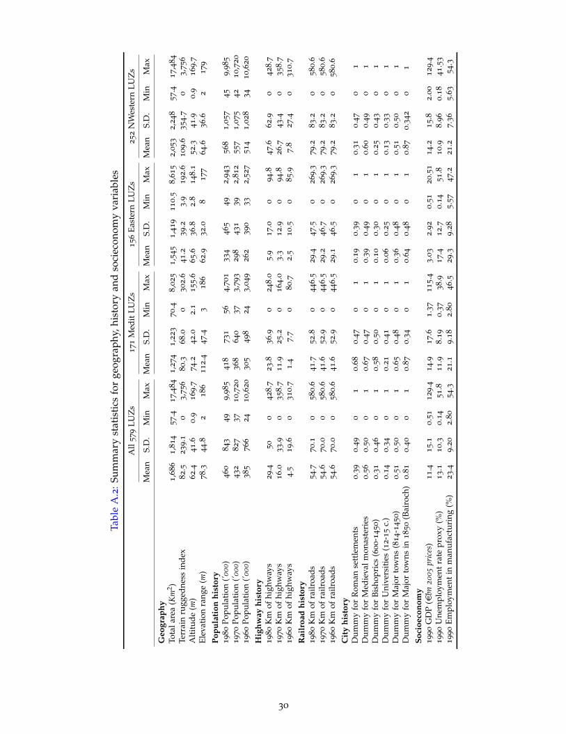
Tabl

eA

.2:S

umm

ary

stat

isti

csfo

rge

ogra

phy,

hist

ory

and

soci

econ

omy

vari

able

s

All

57

9LU

Zs

17

1M

edit

LUZ

s1

56

East

ern

LUZ

s2

52

NW

este

rnLU

Zs

Mea

nS.

D.

Min

Max

Mea

nS.

D.

Min

Max

Mea

nS.

D.

Min

Max

Mea

nS.

D.

Min

Max

Geo

grap

hyTo

tala

rea

(Km

2 )1

,68

61

,81

45

7.4

17,4

84

1,2

74

1,2

23

70.4

8,0

25

1,5

45

1,4

19

11

0.5

8,6

15

2,0

53

2,2

48

57.4

17,4

84

Terr

ain

rugg

edne

ssin

dex

82.5

23

9.1

03,7

56

80

.36

8.0

03

02.6

41.2

39.2

3.9

19

2.6

10

9.6

35

4.7

03,7

56

Alt

itud

e(m

)6

2.4

41.6

0.9

16

9.7

74.2

42

.02.1

15

5.6

65.6

36

.82.8

14

8.1

52.3

41.9

0.9

16

9.7

Elev

atio

nra

nge

(m)

78.3

44

.82

18

61

12.4

47.4

31

86

62.9

32

.08

17

76

4.6

36.6

21

79

Popu

lati

onhi

stor

y1

98

0Po

pula

tion

(’000

)4

60

84

34

99,9

85

41

87

31

56

4,7

01

33

44

65

49

2,9

43

56

81,0

57

45

9,9

85

19

70

Popu

lati

on(’0

00)

43

28

27

37

10,7

20

36

86

40

37

3,7

93

29

84

31

39

2,8

12

55

71,0

75

42

10,7

20

19

60

Popu

lati

on(’0

00)

38

57

66

24

10,6

20

30

54

98

24

3,0

49

26

23

90

33

2,5

27

51

41,0

28

34

10

,62

0

Hig

hway

hist

ory

19

80

Km

ofhi

ghw

ays

29

.45

00

42

8.7

23.8

36.9

02

48.0

5.9

17.0

09

4.8

47.6

62.9

04

28.7

19

70

Km

ofhi

ghw

ays

16

.03

3.9

03

58.7

11.9

25.2

01

64.0

3.3

12.9

09

4.8

26.7

43.4

03

58.7

19

60

Km

ofhi

ghw

ays

4.5

19.6

03

10.7

1.4

7.7

08

0.7

2.5

10.5

08

5.9

7.8

27.4

03

10

.7

Rai

lroa

dhi

stor

y1

98

0K

mof

railr

oads

54

.77

0.1

05

80.6

41.7

52.8

04

46.5

29.4

47

.50

26

9.3

79.2

83

.20

58

0.6

19

70

Km

ofra

ilroa

ds5

4.6

70.0

05

80.6

41.6

52

.90

44

6.5

29.2

46.7

02

69.3

79.2

83

.20

58

0.6

19

60

Km

ofra

ilroa

ds5

4.6

70.0

05

80.6

41.6

52

.90

44

6.5

29.1

46.5

02

69.3

79.2

83

.20

58

0.6

Cit

yhi

stor

yD

umm

yfo

rR

oman

sett

lem

ents

0.3

90.4

90

10.6

80

.47

01

0.1

90.3

90

10.3

10

.47

01

Dum

my

for

Med

ieva

lmon

aste

ries

0.5

60.5

00

10.6

70

.47

01

0.3

90.4

90

10.6

00

.49

01

Dum

my

for

Bish

opri

cs(6

00

-14

50

)0

.31

0.4

60

10.5

80

.50

01

0.1

00.3

00

10.2

50

.43

01

Dum

my

for

Uni

vers

itie

s(1

2-1

5c.

)0

.14

0.3

40

10.2

10

.41

01

0.0

60.2

50

10.1

30

.33

01

Dum

my

for

Maj

orto

wns

(81

4-1

45

0)

0.5

10.5

00

10.6

50

.48

01

0.3

60.4

80

10.5

10

.50

01

Dum

my

for

Maj

orto

wns

in1

85

0(B

airo

ch)

0.8

10.4

00

10.8

70

.34

01

0.6

40

.48

01

0.8

70.3

42

01

Soci

oeco

nom

y1

99

0G

DP

(ebn

2005

pric

es)

11

.41

5.1

0.5

11

29

.41

4.9

17.6

1.3

71

15.4

3.0

32

.92

0.5

12

0.5

11

4.2

15.8

2.0

01

29.4

19

90

Une

mpl

oym

ent

rate

prox

y(%

)1

3.1

10

.30

.14

51.8

11.9

8.1

90.3

73

8.9

17

.41

2.7

0.1

45

1.8

10.9

8.9

60.1

84

1.5

3

19

90

Empl

oym

ent

inm

anuf

actu

ring

(%)

23

.49

.20

2.8

05

4.3

21.1

9.1

82.8

04

6.5

29

.39

.28

5.5

74

7.2

21.2

7.3

65.6

35

4.3

30

Table A.3: Developed land area, fragmentation and surroundings in Europe and its cities

Area (km2) Fragmentation (Lots) Surroundings (% Und.)

1990 2012 1990–2012 1990 2012 1990–2012 1990 2012

Panel A: All developed landEurope-29 185,971 213,307 27,337 (15%) 138,868 162,819 23,951 (17%) 40.2 40.4

All 579 LUZs 88,300 101,043 12,743 (14%) 48,471 56,040 7,569 (16%) 36.3 36.1

171 Medit 17,565 21,136 3,571 (20%) 9,435 10,677 1,242 (13%) 37.7 36.9

156 Eastern 17,814 21,479 3,665 (21%) 12,146 15,598 3,452 (28%) 38.1 40.5

252 NWest 52,921 58,428 5,507 (10%) 26,894 29,765 2,875 (11%) 34.1 32.8

Panel B: Industrial and commercial units landEurope-29 19,850 25,868 6,018 (30%) 26,822 33,901 7,079 (26%) 34.4 34.3

All 579 LUZs 10,711 14,130 3,419 (32%) 12,224 16,245 4,021 (33%) 33.0 31.1

171 Medit 2,747 3,723 976 (36%) 3,021 3,898 877 (29%) 39.7 35.7

156 Eastern 2,465 2,906 441 (18%) 3,064 3,587 523 (17%) 34.9 33.2

252 NWest 5,499 7,501 2,002 (36%) 6,139 8,760 2,621 (43%) 27.2 26.6

Notes: ’Area’ refers to square kilometers of developed land area, ’Fragmentation’ refers to the number of developedland lots, and ’Surroundings’ refers to the % of undeveloped land surrounding developed land. Total areas are:4,851,351 km2 for Europe (29 countries), 976,178 km2 for the 579 LUZs, 217,785 km2 for the 171 Mediterranean cities,241.078 km2 for the 156 Eastern cities, and 517,315 km2 for the 256 Northwestern cities.

31

Appendix B. First-stage and reduced-form results

Table B.1: Modern highway length, historical (rail)roads and residential land in European cities

Regression: FS RF RF RF FS RF RF RF FS RF RF RFLand indicator: All Area Fragm Surr All Area Fragm Surr All Area Fragm Surr

[1] [2] [3] [4] [5] [6] [7] [8] [9] [10] [11] [12]

Panel A: Roman roads Trade routes 1810 Post roadsln(Km of ...) 0.162

a0.002 0.012

b0.004 0.007 -0.002 0.015 0.007

b0.138

b0.002 0.022 0.009

(0.058) (0.004) (0.006) (0.003) (0.121) (0.004) (0.011) (0.003) (0.067) (0.007) (0.017) (0.006)

Adjusted R20.39 0.27 0.30 0.20 0.38 0.27 0.30 0.20 0.38 0.27 0.30 0.21

FS F-statistic 7.88 0.00 4.27

Panel B: 1870 Railroads max(Roman, 1870 Rail) max(Roman, Trade, Post, Rail)ln(Km of ...) 0.193

a -0.001 -0.005 -0.002 0.234a

0.010b

0.005 0.001 0.202a

0.013b

0.035c

0.014b

(0.040) (0.005) (0.019) (0.006) (0.040) (0.004) (0.014) (0.004) (0.058) (0.006) (0.018) (0.006)

Adjusted R20.39 0.27 0.30 0.20 0.39 0.27 0.30 0.20 0.39 0.28 0.31 0.21

FS F-statistic 22.87 33.57 12.12

Notes: First-stage (FS) and Reduced-form (RF) results for regressions in Tables 7, 8 and 9 Panel A Column 5. FSand RF dependent variables are the 1990 log of kilometers of highways and 1990–2012 ∆ln(Residential variable),respectively. ’Area’ refers to square kilometers of residential land area, ’Fragm’ refers to the number of residentialland lots, and ’Surr’ refers to the % of undeveloped land surrounding residential land. 579 observations in eachregression. All regressions include control variables for the 1990 log of residential land area, the 1990 log of thenumber of residential lots, the 1990 log of % of undeveloped land surrounding residential land, geography, history,socioeconomy and country fixed-effects. Robust standard errors clustered by country are in parentheses. a, b, andc indicates significant at 1, 5, and 10 percent level, respectively.

32

Appendix C. The effect of highway ramps

Table C.1: The effect of highway ramps on residential land area in European cities

Dependent variable: 1990–2012 ∆ln(Km2 of residential land area)

Region: Med East NW[1] [2] [3] [4] [5] [6] [7] [8]

Panel A: OLS results1990 ln(Number of highway ramps) 0.026

b0.026

b0.027

b0.011 0.011 0.010 0.010 0.011

(0.011) (0.010) (0.010) (0.007) (0.008) (0.007) (0.008) (0.012)1990 ln(Number of ramps) × Region dummy 0.001 -0.001 0.000

(0.013) (0.012) (0.011)1990 ln(Km2 of residential land area) -0.051

a -0.123b -0.132

b -0.267a -0.268

a -0.275a -0.270

a -0.268a

(0.014) (0.056) (0.054) (0.064) (0.064) (0.060) (0.064) (0.064)

Adjusted R20.59 0.60 0.64 0.69 0.69 0.69 0.69 0.69

Panel B: TSLS results1990 ln(Number of highway ramps) 0.090

b0.077

b0.082

a0.079

b0.077

b0.075

b0.059

c0.096

b

(0.038) (0.033) (0.027) (0.036) (0.034) (0.033) (0.032) (0.042)1990 ln(Number of ramps) × Region dummy 0.018 0.033 -0.045

b

(0.028) (0.027) (0.021)1990 ln(Km2 of residential land area) -0.106

a -0.159a -0.169

a -0.267a -0.268

a -0.272a -0.270

a -0.264a

(0.035) (0.060) (0.054) (0.053) (0.053) (0.048) (0.055) (0.050)

First-stage F-statistic 55.84 43.53 42.22 24.77 23.73 11.89 15.62 12.89

Instrument ln(Km of max(Roman roads, 1870 Railroads))ln(Km) × Region dummy

1990 ln(Number of residential lots) N Y Y Y Y Y Y Y1990 ln(% Undeveloped land surroundings) N Y Y Y Y Y Y YGeography N N Y Y Y Y Y YPopulation history N N N Y Y Y Y YRailroad history N N N Y Y Y Y YCity history N N N Y Y Y Y YSocioeconomy N N N N Y Y Y YRegion dummy N N N N N Y Y YCountry FE Y Y Y Y Y Y Y Y

Notes: 579 observations in each regression. Robust standard errors clustered by country are in parentheses. a, b,and c indicates significant at 1, 5, and 10 percent level, respectively.

33

Appendix D. Results for ’All developed’ and ’Industrial and commercial units’ land

Table D.1: The effect of highways on land area, fragmentation and undeveloped surroundings inEuropean cities: All developed land

Dependent variable: 1990–2012 ∆ln(All developed indicator)

Land indicator: Km2 of land area Number of lots % Und. surroundings

Method: OLS TSLS OLS TSLS OLS TSLS[1] [2] [3] [4] [5] [6]

1990 ln(Km of highways) 0.006 0.044c

0.005 0.073c -0.001 0.044

(0.006) (0.023) (0.006) (0.040) (0.002) (0.030)1990 ln(All developed indicator) -0.284

a -0.298a -0.209

a -0.190a -0.260

a -0.291a

(0.062) (0.059) (0.069) (0.069) (0.059) (0.065)

Adjusted R20.72 0.63 0.52

First-stage F-statistic 37.22 7.73 12.19

Instrument: ln(Km of ...) max(Roman, Rail) Roman roads max(Roman, Trade,Post, Rail)

Notes: 579 observations in each TSLS regression. All regressions include control variables for the 1990 log ofresidential land area, the 1990 log of the number of residential lots, the 1990 log of % of undeveloped landsurrounding residential land, geography, history, socioeconomy and country fixed-effects. Robust standard errorsclustered by country are in parentheses. a, b, and c indicates significant at 1, 5, and 10 percent level, respectively.

Table D.2: The effect of highways on land area, fragmentation and undeveloped surroundings inEuropean cities: Industrial and commercial land

Dependent variable: 1990–2012 ∆ln(Industrial and commercial indicator)

Land indicator: Km2 of land area Number of lots % Und. surroundings

Method: OLS TSLS OLS TSLS OLS TSLS[1] [2] [3] [4] [5] [6]

1990 ln(Highway indicator) 0.009c

0.111c

0.003 0.122c -0.008 0.011

(0.005) (0.062) (0.007) (0.066) (0.005) (0.023)1990 ln(Ind & com indicator) -0.368

a -0.395a -0.369

a -0.339a -0.441

a -0.447a

(0.058) (0.077) (0.062) (0.054) (0.056) (0.052)

Adjusted R20.67 0.69 0.50

First-stage F-statistic 32.19 32.19 32.19

Instrument ln(Km of max(Roman roads, Trade routes, 1810 Post roads, 1870 Railroads))

Notes: 579 observations in each TSLS regression. All regressions include control variables for the 1990 log ofresidential land area, the 1990 log of the number of residential lots, the 1990 log of % of undeveloped landsurrounding residential land, geography, history, socioeconomy and country fixed-effects. Robust standard errorsclustered by country are in parentheses. a, b, and c indicates significant at 1, 5, and 10 percent level, respectively.

34

Appendix E. Joint effect of 1990 highways and 1990-2000/10 improvements

Table E.1: The joint effect of 1990 highways and its 1990-2000/10 improvementson land area, fragmentation and undeveloped surroundings in European cities

Dependent variable: 1990–2012 ∆ln(Residential indicator)

Land indicator: Km2 of land area Number of lots % Und. surroundings

[1] [2] [3] [4] [5] [6]

Panel A: OLS results2000 ln(Km of highways) 0.005 0.006 0.002

(0.007) (0.008) (0.003)2010 ln(Km of highways) 0.004 0.006 0.002

(0.006) (0.008) (0.004)

Adjusted R20.69 0.69 0.64 0.64 0.48 0.48

Panel B: TSLS results2000 ln(Km of highways) 0.035

b0.156

c0.060

c

(0.018) (0.097) (0.037)2010 ln(Km of highways) 0.031

b0.110

b0.043

b

(0.013) (0.050) (0.017)

First-stage F-statistic 34.16 47.72 9.15 25.34 9.15 25.34

Instrument: ln(Km of ...) max(Roman, Rail) max(Roman roads, Trade, 1810 Post, 1870 Rail)

Notes: 579 observations in each TSLS regression. All regressions include control variables for the 1990 log ofresidential land area, the 1990 log of the number of residential lots, the 1990 log of % of undeveloped landsurrounding residential land, geography, history, socioeconomy and country fixed-effects. Robust standard errorsclustered by country are in parentheses. a, b, and c indicates significant at 1, 5, and 10 percent level, respectively.

35

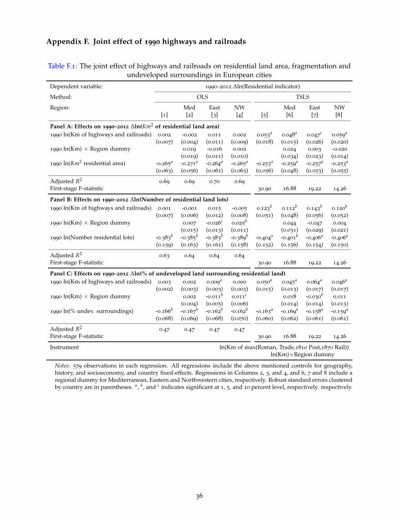
Appendix F. Joint effect of 1990 highways and railroads

Table F.1: The joint effect of highways and railroads on residential land area, fragmentation andundeveloped surroundings in European cities

Dependent variable: 1990–2012 ∆ln(Residential indicator)

Method: OLS TSLS

Region: Med East NW Med East NW[1] [2] [3] [4] [5] [6] [7] [8]

Panel A: Effects on 1990–2012 ∆ln(Km2 of residential land area)1990 ln(Km of highways and railroads) 0.002 -0.002 0.011 0.002 0.053

a0.048

a0.047

c0.059

a

(0.007) (0.004) (0.011) (0.009) (0.018) (0.015) (0.026) (0.020)1990 ln(Km) × Region dummy 0.019 -0.016 0.002 0.024 0.003 -0.020

(0.019) (0.011) (0.010) (0.034) (0.023) (0.014)1990 ln(Km2 residential area) -0.265

a -0.271a -0.264

a -0.265a -0.253

a -0.259a -0.257

a -0.253a

(0.063) (0.056) (0.061) (0.063) (0.056) (0.048) (0.053) (0.055)

Adjusted R20.69 0.69 0.70 0.69

First-stage F-statistic 30.90 16.88 19.22 14.26

Panel B: Effects on 1990–2012 ∆ln(Number of residential land lots)1990 ln(Km of highways and railroads) 0.001 -0.001 0.015 -0.005 0.123

b0.112

b0.143

b0.120

b

(0.007) (0.006) (0.012) (0.008) (0.051) (0.048) (0.056) (0.052)1990 ln(Km) × Region dummy 0.007 -0.026

c0.025

b0.044 -0.047 0.004

(0.015) (0.013) (0.011) (0.031) (0.029) (0.021)1990 ln(Number residential lots) -0.383

b -0.385b -0.383

b -0.389b -0.404

a -0.401b -0.406

a -0.406a

(0.159) (0.163) (0.161) (0.158) (0.152) (0.156) (0.154) (0.150)

Adjusted R20.63 0.64 0.64 0.64

First-stage F-statistic 30.90 16.88 19.22 14.26

Panel C: Effects on 1990–2012 ∆ln(% of undeveloped land surrounding residential land)1990 ln(Km of highways and railroads) 0.003 0.002 0.009

a0.000 0.050

a0.045

a0.064

a0.046

a

(0.002) (0.003) (0.003) (0.003) (0.015) (0.013) (0.017) (0.017)1990 ln(Km) × Region dummy 0.002 -0.011

b0.011

c0.018 -0.030

b0.011

(0.004) (0.005) (0.006) (0.014) (0.014) (0.013)1990 ln(% undev. surroundings) -0.166

b -0.167b -0.162

b -0.162b -0.163

a -0.169a -0.158

a -0.159a

(0.068) (0.069) (0.068) (0.070) (0.060) (0.062) (0.061) (0.061)

Adjusted R20.47 0.47 0.47 0.47

First-stage F-statistic 30.90 16.88 19.22 14.26

Instrument ln(Km of max(Roman, Trade,1810 Post,1870 Rail))ln(Km)×Region dummy

Notes: 579 observations in each regression. All regressions include the above mentioned controls for geography,history, and socioeconomy, and country fixed-effects. Regressions in Columns 2, 3, and 4, and 6, 7 and 8 include aregional dummy for Mediterranean, Eastern and Northwestern cities, respectively. Robust standard errors clusteredby country are in parentheses. a, b, and c indicates significant at 1, 5, and 10 percent level, respectively. respectively.

36

IEB Working Papers

2013

2013/1, Sánchez-Vidal, M.; González-Val, R.; Viladecans-Marsal, E.: "Sequential city growth in the US: does age

matter?"

2013/2, Hortas Rico, M.: "Sprawl, blight and the role of urban containment policies. Evidence from US cities"

2013/3, Lampón, J.F.; Cabanelas-Lorenzo, P-; Lago-Peñas, S.: "Why firms relocate their production overseas? The

answer lies inside: corporate, logistic and technological determinants"

2013/4, Montolio, D.; Planells, S.: "Does tourism boost criminal activity? Evidence from a top touristic country"

2013/5, Garcia-López, M.A.; Holl, A.; Viladecans-Marsal, E.: "Suburbanization and highways: when the Romans, the

Bourbons and the first cars still shape Spanish cities"

2013/6, Bosch, N.; Espasa, M.; Montolio, D.: "Should large Spanish municipalities be financially compensated? Costs

and benefits of being a capital/central municipality"

2013/7, Escardíbul, J.O.; Mora, T.: "Teacher gender and student performance in mathematics. Evidence from

Catalonia"

2013/8, Arqué-Castells, P.; Viladecans-Marsal, E.: "Banking towards development: evidence from the Spanish banking

expansion plan"

2013/9, Asensio, J.; Gómez-Lobo, A.; Matas, A.: "How effective are policies to reduce gasoline consumption?

Evaluating a quasi-natural experiment in Spain"

2013/10, Jofre-Monseny, J.: "The effects of unemployment benefits on migration in lagging regions"

2013/11, Segarra, A.; García-Quevedo, J.; Teruel, M.: "Financial constraints and the failure of innovation projects"

2013/12, Jerrim, J.; Choi, A.: "The mathematics skills of school children: How does England compare to the high

performing East Asian jurisdictions?"

2013/13, González-Val, R.; Tirado-Fabregat, D.A.; Viladecans-Marsal, E.: "Market potential and city growth: Spain

1860-1960"

2013/14, Lundqvist, H.: "Is it worth it? On the returns to holding political office"

2013/15, Ahlfeldt, G.M.; Maennig, W.: "Homevoters vs. leasevoters: a spatial analysis of airport effects"

2013/16, Lampón, J.F.; Lago-Peñas, S.: "Factors behind international relocation and changes in production geography

in the European automobile components industry"

2013/17, Guío, J.M.; Choi, A.: "Evolution of the school failure risk during the 2000 decade in Spain: analysis of Pisa

results with a two-level logistic mode"

2013/18, Dahlby, B.; Rodden, J.: "A political economy model of the vertical fiscal gap and vertical fiscal imbalances in

a federation"

2013/19, Acacia, F.; Cubel, M.: "Strategic voting and happiness"

2013/20, Hellerstein, J.K.; Kutzbach, M.J.; Neumark, D.: "Do labor market networks have an important spatial

dimension?"

2013/21, Pellegrino, G.; Savona, M.: "Is money all? Financing versus knowledge and demand constraints to innovation"

2013/22, Lin, J.: "Regional resilience"

2013/23, Costa-Campi, M.T.; Duch-Brown, N.; García-Quevedo, J.: "R&D drivers and obstacles to innovation in the

energy industry"

2013/24, Huisman, R.; Stradnic, V.; Westgaard, S.: "Renewable energy and electricity prices: indirect empirical

evidence from hydro power"

2013/25, Dargaud, E.; Mantovani, A.; Reggiani, C.: "The fight against cartels: a transatlantic perspective"

2013/26, Lambertini, L.; Mantovani, A.: "Feedback equilibria in a dynamic renewable resource oligopoly: pre-emption,

voracity and exhaustion"

2013/27, Feld, L.P.; Kalb, A.; Moessinger, M.D.; Osterloh, S.: "Sovereign bond market reactions to fiscal rules and no-

bailout clauses – the Swiss experience"

2013/28, Hilber, C.A.L.; Vermeulen, W.: "The impact of supply constraints on house prices in England"

2013/29, Revelli, F.: "Tax limits and local democracy"

2013/30, Wang, R.; Wang, W.: "Dress-up contest: a dark side of fiscal decentralization"

2013/31, Dargaud, E.; Mantovani, A.; Reggiani, C.: "The fight against cartels: a transatlantic perspective"

2013/32, Saarimaa, T.; Tukiainen, J.: "Local representation and strategic voting: evidence from electoral boundary

reforms"

2013/33, Agasisti, T.; Murtinu, S.: "Are we wasting public money? No! The effects of grants on Italian university

students’ performances"

2013/34, Flacher, D.; Harari-Kermadec, H.; Moulin, L.: "Financing higher education: a contributory scheme"

2013/35, Carozzi, F.; Repetto, L.: "Sending the pork home: birth town bias in transfers to Italian municipalities"

2013/36, Coad, A.; Frankish, J.S.; Roberts, R.G.; Storey, D.J.: "New venture survival and growth: Does the fog lift?"

IEB Working Papers

2013/37, Giulietti, M.; Grossi, L.; Waterson, M.: "Revenues from storage in a competitive electricity market: Empirical

evidence from Great Britain"

2014

2014/1, Montolio, D.; Planells-Struse, S.: "When police patrols matter. The effect of police proximity on citizens’ crime

risk perception"

2014/2, Garcia-López, M.A.; Solé-Ollé, A.; Viladecans-Marsal, E.: "Do land use policies follow road construction?"

2014/3, Piolatto, A.; Rablen, M.D.: "Prospect theory and tax evasion: a reconsideration of the Yitzhaki puzzle"

2014/4, Cuberes, D.; González-Val, R.: "The effect of the Spanish Reconquest on Iberian Cities"

2014/5, Durán-Cabré, J.M.; Esteller-Moré, E.: "Tax professionals' view of the Spanish tax system: efficiency, equity

and tax planning"

2014/6, Cubel, M.; Sanchez-Pages, S.: "Difference-form group contests"

2014/7, Del Rey, E.; Racionero, M.: "Choosing the type of income-contingent loan: risk-sharing versus risk-pooling"

2014/8, Torregrosa Hetland, S.: "A fiscal revolution? Progressivity in the Spanish tax system, 1960-1990"

2014/9, Piolatto, A.: "Itemised deductions: a device to reduce tax evasion"

2014/10, Costa, M.T.; García-Quevedo, J.; Segarra, A.: "Energy efficiency determinants: an empirical analysis of

Spanish innovative firms"

2014/11, García-Quevedo, J.; Pellegrino, G.; Savona, M.: "Reviving demand-pull perspectives: the effect of demand

uncertainty and stagnancy on R&D strategy"

2014/12, Calero, J.; Escardíbul, J.O.: "Barriers to non-formal professional training in Spain in periods of economic

growth and crisis. An analysis with special attention to the effect of the previous human capital of workers"

2014/13, Cubel, M.; Sanchez-Pages, S.: "Gender differences and stereotypes in the beauty"

2014/14, Piolatto, A.; Schuett, F.: "Media competition and electoral politics"

2014/15, Montolio, D.; Trillas, F.; Trujillo-Baute, E.: "Regulatory environment and firm performance in EU

telecommunications services"

2014/16, Lopez-Rodriguez, J.; Martinez, D.: "Beyond the R&D effects on innovation: the contribution of non-R&D

activities to TFP growth in the EU"

2014/17, González-Val, R.: "Cross-sectional growth in US cities from 1990 to 2000"

2014/18, Vona, F.; Nicolli, F.: "Energy market liberalization and renewable energy policies in OECD countries"

2014/19, Curto-Grau, M.: "Voters’ responsiveness to public employment policies"

2014/20, Duro, J.A.; Teixidó-Figueras, J.; Padilla, E.: "The causal factors of international inequality in co2 emissions

per capita: a regression-based inequality decomposition analysis"

2014/21, Fleten, S.E.; Huisman, R.; Kilic, M.; Pennings, E.; Westgaard, S.: "Electricity futures prices: time varying

sensitivity to fundamentals"

2014/22, Afcha, S.; García-Quevedo, J,: "The impact of R&D subsidies on R&D employment composition"

2014/23, Mir-Artigues, P.; del Río, P.: "Combining tariffs, investment subsidies and soft loans in a renewable electricity

deployment policy"

2014/24, Romero-Jordán, D.; del Río, P.; Peñasco, C.: "Household electricity demand in Spanish regions. Public policy

implications"

2014/25, Salinas, P.: "The effect of decentralization on educational outcomes: real autonomy matters!"

2014/26, Solé-Ollé, A.; Sorribas-Navarro, P.: "Does corruption erode trust in government? Evidence from a recent

surge of local scandals in Spain"

2014/27, Costas-Pérez, E.: "Political corruption and voter turnout: mobilization or disaffection?"

2014/28, Cubel, M.; Nuevo-Chiquero, A.; Sanchez-Pages, S.; Vidal-Fernandez, M.: "Do personality traits affect

productivity? Evidence from the LAB"

2014/29, Teresa Costa, M.T.; Trujillo-Baute, E.: "Retail price effects of feed-in tariff regulation"

2014/30, Kilic, M.; Trujillo-Baute, E.: "The stabilizing effect of hydro reservoir levels on intraday power prices under

wind forecast errors"

2014/31, Costa-Campi, M.T.; Duch-Brown, N.: "The diffusion of patented oil and gas technology with environmental

uses: a forward patent citation analysis"

2014/32, Ramos, R.; Sanromá, E.; Simón, H.: "Public-private sector wage differentials by type of contract: evidence

from Spain"

2014/33, Backus, P.; Esteller-Moré, A.: "Is income redistribution a form of insurance, a public good or both?"

2014/34, Huisman, R.; Trujillo-Baute, E.: "Costs of power supply flexibility: the indirect impact of a Spanish policy

change"

IEB Working Papers

2014/35, Jerrim, J.; Choi, A.; Simancas Rodríguez, R.: "Two-sample two-stage least squares (TSTSLS) estimates of

earnings mobility: how consistent are they?"

2014/36, Mantovani, A.; Tarola, O.; Vergari, C.: "Hedonic quality, social norms, and environmental campaigns"

2014/37, Ferraresi, M.; Galmarini, U.; Rizzo, L.: "Local infrastructures and externalities: Does the size matter?"

2014/38, Ferraresi, M.; Rizzo, L.; Zanardi, A.: "Policy outcomes of single and double-ballot elections"

2015

2015/1, Foremny, D.; Freier, R.; Moessinger, M-D.; Yeter, M.: "Overlapping political budget cycles in the legislative

and the executive"

2015/2, Colombo, L.; Galmarini, U.: "Optimality and distortionary lobbying: regulating tobacco consumption"

2015/3, Pellegrino, G.: "Barriers to innovation: Can firm age help lower them?"

2015/4, Hémet, C.: "Diversity and employment prospects: neighbors matter!"

2015/5, Cubel, M.; Sanchez-Pages, S.: "An axiomatization of difference-form contest success functions"

2015/6, Choi, A.; Jerrim, J.: "The use (and misuse) of Pisa in guiding policy reform: the case of Spain"

2015/7, Durán-Cabré, J.M.; Esteller-Moré, A.; Salvadori, L.: "Empirical evidence on tax cooperation between sub-

central administrations"

2015/8, Batalla-Bejerano, J.; Trujillo-Baute, E.: "Analysing the sensitivity of electricity system operational costs to

deviations in supply and demand"

2015/9, Salvadori, L.: "Does tax enforcement counteract the negative effects of terrorism? A case study of the Basque

Country"

2015/10, Montolio, D.; Planells-Struse, S.: "How time shapes crime: the temporal impacts of football matches on crime"

2015/11, Piolatto, A.: "Online booking and information: competition and welfare consequences of review aggregators"

2015/12, Boffa, F.; Pingali, V.; Sala, F.: "Strategic investment in merchant transmission: the impact of capacity

utilization rules"

2015/13, Slemrod, J.: "Tax administration and tax systems"

2015/14, Arqué-Castells, P.; Cartaxo, R.M.; García-Quevedo, J.; Mira Godinho, M.: "How inventor royalty shares

affect patenting and income in Portugal and Spain"

2015/15, Montolio, D.; Planells-Struse, S.: "Measuring the negative externalities of a private leisure activity: hooligans

and pickpockets around the stadium"

2015/16, Batalla-Bejerano, J.; Costa-Campi, M.T.; Trujillo-Baute, E.: "Unexpected consequences of liberalisation:

metering, losses, load profiles and cost settlement in Spain’s electricity system"

2015/17, Batalla-Bejerano, J.; Trujillo-Baute, E.: "Impacts of intermittent renewable generation on electricity system

costs"

2015/18, Costa-Campi, M.T.; Paniagua, J.; Trujillo-Baute, E.: "Are energy market integrations a green light for FDI?"

2015/19, Jofre-Monseny, J.; Sánchez-Vidal, M.; Viladecans-Marsal, E.: "Big plant closures and agglomeration

economies"

2015/20, Garcia-López, M.A.; Hémet, C.; Viladecans-Marsal, E.: "How does transportation shape intrametropolitan

growth? An answer from the regional express rail"

2015/21, Esteller-Moré, A.; Galmarini, U.; Rizzo, L.: "Fiscal equalization under political pressures"

2015/22, Escardíbul, J.O.; Afcha, S.: "Determinants of doctorate holders’ job satisfaction. An analysis by employment

sector and type of satisfaction in Spain"

2015/23, Aidt, T.; Asatryan, Z.; Badalyan, L.; Heinemann, F.: "Vote buying or (political) business (cycles) as usual?"

2015/24, Albæk, K.: "A test of the ‘lose it or use it’ hypothesis in labour markets around the world"

2015/25, Angelucci, C.; Russo, A.: "Petty corruption and citizen feedback"

2015/26, Moriconi, S.; Picard, P.M.; Zanaj, S.: "Commodity taxation and regulatory competition"

2015/27, Brekke, K.R.; Garcia Pires, A.J.; Schindler, D.; Schjelderup, G.: "Capital taxation and imperfect

competition: ACE vs. CBIT"

2015/28, Redonda, A.: "Market structure, the functional form of demand and the sensitivity of the vertical reaction

function"

2015/29, Ramos, R.; Sanromá, E.; Simón, H.: "An analysis of wage differentials between full-and part-time workers in

Spain"

2015/30, Garcia-López, M.A.; Pasidis, I.; Viladecans-Marsal, E.: "Express delivery to the suburbs the effects of

transportation in Europe’s heterogeneous cities"

2015/31, Torregrosa, S.: "Bypassing progressive taxation: fraud and base erosion in the Spanish income tax (1970-

2001)"

IEB Working Papers

2015/32, Choi, H.; Choi, A.: "When one door closes: the impact of the hagwon curfew on the consumption of private

tutoring in the republic of Korea"

2015/33, Escardíbul, J.O.; Helmy, N.: "Decentralisation and school autonomy impact on the quality of education: the

case of two MENA countries"

2015/34, González-Val, R.; Marcén, M.: "Divorce and the business cycle: a cross-country analysis"

2015/35, Calero, J.; Choi, A.: "The distribution of skills among the European adult population and unemployment: a

comparative approach"

2015/36, Mediavilla, M.; Zancajo, A.: "Is there real freedom of school choice? An analysis from Chile"

2015/37, Daniele, G.: "Strike one to educate one hundred: organized crime, political selection and politicians’ ability"

2015/38, González-Val, R.; Marcén, M.: "Regional unemployment, marriage, and divorce"

2015/39, Foremny, D.; Jofre-Monseny, J.; Solé-Ollé, A.: "‘Hold that ghost’: using notches to identify manipulation of

population-based grants"

2015/40, Mancebón, M.J.; Ximénez-de-Embún, D.P.; Mediavilla, M.; Gómez-Sancho, J.M.: "Does educational

management model matter? New evidence for Spain by a quasiexperimental approach"

2015/41, Daniele, G.; Geys, B.: "Exposing politicians’ ties to criminal organizations: the effects of local government

dissolutions on electoral outcomes in Southern Italian municipalities"

2015/42, Ooghe, E.: "Wage policies, employment, and redistributive efficiency"

2016

2016/1, Galletta, S.: "Law enforcement, municipal budgets and spillover effects: evidence from a quasi-experiment in

Italy"

2016/2, Flatley, L.; Giulietti, M.; Grossi, L.; Trujillo-Baute, E.; Waterson, M.: "Analysing the potential economic

value of energy storage"

2016/3, Calero, J.; Murillo Huertas, I.P.; Raymond Bara, J.L.: "Education, age and skills: an analysis using the

PIAAC survey"

2016/4, Costa-Campi, M.T.; Daví-Arderius, D.; Trujillo-Baute, E.: "The economic impact of electricity losses"

2016/5, Falck, O.; Heimisch, A.; Wiederhold, S.: "Returns to ICT skills"

2016/6, Halmenschlager, C.; Mantovani, A.: "On the private and social desirability of mixed bundling in

complementary markets with cost savings"

2016/7, Choi, A.; Gil, M.; Mediavilla, M.; Valbuena, J.: "Double toil and trouble: grade retention and academic

performance"

2016/8, González-Val, R.: "Historical urban growth in Europe (1300–1800)"

2016/9, Guio, J.; Choi, A.; Escardíbul, J.O.: "Labor markets, academic performance and the risk of school dropout:

evidence for Spain"

2016/10, Bianchini, S.; Pellegrino, G.; Tamagni, F.: "Innovation strategies and firm growth"

2016/11, Jofre-Monseny, J.; Silva, J.I.; Vázquez-Grenno, J.: "Local labor market effects of public employment"

2016/12, Sanchez-Vidal, M.: "Small shops for sale! The effects of big-box openings on grocery stores"

2016/13, Costa-Campi, M.T.; García-Quevedo, J.; Martínez-Ros, E.: "What are the determinants of investment in

environmental R&D?"

2016/14, García-López, M.A; Hémet, C.; Viladecans-Marsal, E.: "Next train to the polycentric city: The effect of

railroads on subcenter formation"

2016/15, Matas, A.; Raymond, J.L.; Dominguez, A.: "Changes in fuel economy: An analysis of the Spanish car market"

2016/16, Leme, A.; Escardíbul, J.O.: "The effect of a specialized versus a general upper secondary school curriculum on

students’ performance and inequality. A difference-in-differences cross country comparison"

2016/17, Scandurra, R.I.; Calero, J.: “Modelling adult skills in OECD countries”

2016/18, Fernández-Gutiérrez, M.; Calero, J.: “Leisure and education: insights from a time-use analysis”

2016/19, Del Rio, P.; Mir-Artigues, P.; Trujillo-Baute, E.: “Analysing the impact of renewable energy regulation on

retail electricity prices”

2016/20, Taltavull de la Paz, P.; Juárez, F.; Monllor, P.: “Fuel Poverty: Evidence from housing perspective”

2016/21, Ferraresi, M.; Galmarini, U.; Rizzo, L.; Zanardi, A.: “Switch towards tax centralization in Italy: A wake up

for the local political budget cycle”

2016/22, Ferraresi, M.; Migali, G.; Nordi, F.; Rizzo, L.: “Spatial interaction in local expenditures among Italian

municipalities: evidence from Italy 2001-2011”

2016/23, Daví-Arderius, D.; Sanin, M.E.; Trujillo-Baute, E.: “CO2 content of electricity losses”

IEB Working Papers

2016/24, Arqué-Castells, P.; Viladecans-Marsal, E.: “Banking the unbanked: Evidence from the Spanish banking

expansion plan“

2016/25 Choi, Á.; Gil, M.; Mediavilla, M.; Valbuena, J.: “The evolution of educational inequalities in Spain: Dynamic

evidence from repeated cross-sections”

2016/26, Brutti, Z.: “Cities drifting apart: Heterogeneous outcomes of decentralizing public education”

2016/27, Backus, P.; Cubel, M.; Guid, M.; Sánchez-Pages, S.; Lopez Manas, E.: “Gender, competition and

performance: evidence from real tournaments”

2016/28, Costa-Campi, M.T.; Duch-Brown, N.; García-Quevedo, J.: “Innovation strategies of energy firms”

2016/29, Daniele, G.; Dipoppa, G.: “Mafia, elections and violence against politicians”

2016/30, Di Cosmo, V.; Malaguzzi Valeri, L.: “Wind, storage, interconnection and the cost of electricity”

2017

2017/1, González Pampillón, N.; Jofre-Monseny, J.; Viladecans-Marsal, E.: "Can urban renewal policies reverse

neighborhood ethnic dynamics?”

2017/2, Gómez San Román, T.: "Integration of DERs on power systems: challenges and opportunities”

2017/3, Bianchini, S.; Pellegrino, G.: "Innovation persistence and employment dynamics”

2017/4, Curto‐Grau, M.; Solé‐Ollé, A.; Sorribas‐Navarro, P.: "Does electoral competition curb party favoritism?”

2017/5, Solé‐Ollé, A.; Viladecans-Marsal, E.: "Housing booms and busts and local fiscal policy”

2017/6, Esteller, A.; Piolatto, A.; Rablen, M.D.: "Taxing high-income earners: Tax avoidance and mobility”

2017/7, Combes, P.P.; Duranton, G.; Gobillon, L.: "The production function for housing: Evidence from France”

2017/8, Nepal, R.; Cram, L.; Jamasb, T.; Sen, A.: "Small systems, big targets: power sector reforms and renewable

energy development in small electricity systems”

2017/9, Carozzi, F.; Repetto, L.: "Distributive politics inside the city? The political economy of Spain’s plan E”

2017/10, Neisser, C.: "The elasticity of taxable income: A meta-regression analysis”

2017/11, Baker, E.; Bosetti, V.; Salo, A.: "Finding common ground when experts disagree: robust portfolio decision

analysis”

2017/12, Murillo, I.P; Raymond, J.L; Calero, J.: "Efficiency in the transformation of schooling into competences:

A cross-country analysis using PIAAC data”

2017/13, Ferrer-Esteban, G.; Mediavilla, M.: "The more educated, the more engaged? An analysis of social capital and

education”

2017/14, Sanchis-Guarner, R.: "Decomposing the impact of immigration on house prices”

2017/15, Schwab, T.; Todtenhaupt, M.: "Spillover from the haven: Cross-border externalities of patent box regimes

within multinational firms”

2017/16, Chacón, M.; Jensen, J.: "The institutional determinants of Southern secession”

2017/17, Gancia, G.; Ponzetto, G.A.M.; Ventura, J.: "Globalization and political structure”

2017/18, González-Val, R.: "City size distribution and space”

2017/19, García-Quevedo, J.; Mas-Verdú, F.; Pellegrino, G.: "What firms don’t know can hurt them: Overcoming a

lack of information on technology”

2017/20, Costa-Campi, M.T.; García-Quevedo, J.: "Why do manufacturing industries invest in energy R&D?”

2017/21, Costa-Campi, M. T.; García-Quevedo, J.; Trujillo-Baute, E.: "Electricity regulation and economic growth”

2018

2018/1, Boadway, R.; Pestieau, P.: "The tenuous case for an annual wealth tax”

Cities

ieb@ub.edu

www.ieb.edu