Identification of MIMO linear models: introduction to subspace methods · 2017-11-20 · Identification of MIMO linear models: introduction to subspace methods Marco Lovera Dipartimento

Identification of MIMO linear models: introduction to subspace methods

Marco LoveraDipartimento di Scienze e Tecnologie AerospazialiPolitecnico di [email protected]

State space identification from impulse response data

9/9/2015 - 3-

Ho-Kalman realisation theory

Consider the finite dimensional,

linear time-invariant (LTI) state space model:

Realisation: the problem of computing [A,B,C,D] or an

equivalent realisation for the system, from the

impulse response (Markov parameters) of the system:

9/9/2015 - 4-

Ho-Kalman realisation theory (cont.d)

A few definitions:

Extended observability matrix:

Extended controllability matrix:

9/9/2015 - 5-


Hankel matrix

9/9/2015 - 6-


Properties of the Hankel matrix:

Hi,j, i,j ¸ n, has rank n iff h(t) admits an nth order [A,B,C,D] realisation;

Hi,j can be equivalently written as

9/9/2015 - 7-


The realisation can be constructed as follows:

Let D=h(0);

Construct the Hankel matrix Hi,j from h(1), h(2), …;

Factor the Hankel matrix to get Γi and ∆j;

Let C=first l rows of Γi;

Let B=first m columns of ∆j;

Compute A exploiting shift invariance, i.e., solving

9/9/2015 - 8-

Kung’s algorithm (1978)

What if noisy measurements of h(t) are available?

Idea:

Construct the noisy Hankel matrix \hat Hi,j

Factor the matrix using the SVD:

Estimate Hi,j as the best rank n approximation:

9/9/2015 - 9-

Experimental example

Model for a Peltier cell (n=4, i=20)

Identification and control of rotary wing aircraft

Subspace Model Identification: deterministic case

9/9/2015 - 11-

The data equation

Note that we can write the following equation (i > n)

which describes the system over a window of finite

length.

9/9/2015 Identification and control of rotary wing aircraft- 12-

The data equation (cont.d)

Repeating for various initial times we get the data

equation

where Yt,i,j, Ut,i,j are Hankel matrices:

and Xt,j is defined as


The MOESP algorithm (Verhaegen and Dewilde 1991):

1. Construct projection Π? such that Ut,i,j Π? =0

2. Project data equation using Π? to recover column space of Γi

3. Construct a basis for the column space of ΓI and estimate A and C.

4. Solve LS problem for estimation of B and D.

Orthogonal projection algorithm


Computing the projection Π?

We look for Π? such that Ut,i,j Π? =0.

The solution is given by

since in fact

Note that constructing Π? requires

to be nonsingular.


The projection Π? can be computed and implemented

via the RQ factorisation:

which can be written as

and therefore

Implementation of the projection


Elimination of HiUt,i,j

Therefore, considering the equation

and right-multiplying by Q2T one gets

so R22, of dimension (il £ il) and computed from data

only, contains information on Γi.

Under what conditions range(R22)=range(Γi)?


A rank condition

Theorem 1: if u(t) is such that

then

Problem: this is not yet an identifiability condition,

since it depends on the state.

However, it implies the following.


An identifiability condition

Theorem 2 (Jansson 1997):

if the input u is persistently exciting of order n+i,

then

(i.e., the rank condition of Theorem 1 holds).


Determination of the column space of Γi

Rank reduction of estimated column space of Γi

performed via singular value decomposition of R22.

Under p.e. assumptions, rank(R22=n), so

The inspection of the singular values provides

information about model order.


Estimation of A and C

Let C=first l rows of computed Γi;

Compute A exploiting shift invariance, i.e., solving

the system of linear equations


A simple example (Van Der Veen et al. 1993)

Consider the LTI system (|α|<1)

and apply the input sequence (x(1)=0)

that gives the corresponding output sequence


A simple example (cont.d)

Choosing i=2 and j=3 we can construct the compound

matrix

and computing the RQ factorisation we get


A simple example (cont.d)

We can now factor R22 as :

So

and finally


A numerical example

Consider the order 2 system

and measure the response to a 500 samples realisation

of white gaussian noise.


I/O data


Construction of R22 and SVD

Utij and Ytij are constructed with i=10 and j=490, so R22

is 10 £ 10. Its singular values are given by


Estimated A and C

Numerical results of the estimation procedure:

Note that

The computed A and C are in a different state space basis from the original system;

They are equivalent to the original A and C;

Question: what determines the basis of the estimated matrices?


MATLAB code for the estimation of A and C

function [A,C]=omoesp(u,y,i,j,n);

sy=size(y);su=size(u);

datalen=min([max(sy) max(su)]);

m=min(su); l=min(sy);

H=[];

for ii=1:i

H=[H u(ii:ii+j-1,:)];

end

for ii=1:i

H=[H y(ii:ii+j-1,:)];

end

R=triu(qr(H))';

R22=R(m*i+1:(m+l)*i,m*i+1:(m+l)*i);

[U,S,Vt]=svd(R22);

Un=U(:,1:n);

C=Un(1:l,:);

A=Un(1:l*(i-1),:)\Un(l+1:l*i,:);


Estimation of B and D

The output of the identified model is given by:

we aim at writing the above as a linear regression in

the elements of B and D:

where for X 2 R(m £ n)

For this, we need to introduce Kronecker products.


The Kronecker product

Let A 2 R(m £ n) and B 2 R(r £ s), then the (mr £ ns)

matrix

is called the Kronecker product of A and B.


vec operation and Kronecker product

There is a connection between Kronecker products and

the vec operation.

Let A 2 R(m £ n), B 2 R(n £ o), C 2 R(o £ p), then


Estimation of B and D (cont.d)

Using Kronecker products the output of the identified

model

can be written as

so that B and D can be obtained from:

which is clearly a least squares problem in B and D.


Subspace Model Identification: output error case


SMI: output error case



with the measurement equation

where v is a zero-mean, white measurement noise,

uncorrelated with u.

We want to analyse the effect of v on the identification

algorithm we studied in the deterministic case.


The data equation with measurement error

When adding measurement noise the data equation

becomes

where Vt,i,j is defined as


As in the deterministic case, we:

Construct projection Π? such that Ut,i,j Π? =0

Project data equation using Π? to recover column space of Γi

Using the RQ factorisation we obtain now

Effect of measurement noise


Asymptotic properties of R22

Can we use R22 to estimate the observability subspace?

Theorem 3:

if v ' WN(0, σ2I) and u is p.e. of order n+i, then

and


A numerical example

Consider again the order n=2 system

and measure the response to a 500 samples realisation

of white gaussian noise, subject to v ' (0,0.01).

We repeat the identification 1000 times, with

different realisations of the noise v to assess the

average effect of measurement noise.


I/O data

0 50 100 150 200 250 300 350 400 450 500-3

-2

-1

0

1

2

3

Inpu

t u

0 50 100 150 200 250 300 350 400 450 500-8

-6

-4

-2

0

2

4

6

Out

put

y an

d no

ise

v


Construction of R22 and SVD

R22 is constructed with i=10 and j=490.

Its singular values are given by

1 2 3 4 5 6 7 8 9 100

10

20

30

40

50

60

70

80

Sin

gula

r va

lues

of

R22


Estimated eigenvalues of A

0 100 200 300 400 500 600 700 800 900 10000.25

0.3

0.35

0.4

0.45

0.5

0.55

0.6

0.65

0.7

0.75

Est

imat

ed e

igen

valu

es o

f A


Subspace Model Identification: the general case


SMI: the general case



with the measurement equation

with w and v zero-mean white noises, uncorrelated

with u.

Does the orthogonal projection algorithm still work?


Example

Consider the n=1 system A=0.7; B=1; C=1; D=0; and

compare the performance of the SMI algorithm with

and without process noise w:

0 100 200 300 400 500 600 700 800 900 10000.685

0.69

0.695

0.7

0.705

0.71

0.715

0.72

Est

imat

ed e

igen

valu

es o

f A

w=0

0 100 200 300 400 500 600 700 800 900 10000.685

0.69

0.695

0.7

0.705

0.71

0.715

0.72

0.725

Est

imat

ed e

igen

valu

es o

f A

w ≠ 0


What happened?

When process noise is present, the data equation

becomes

and therefore the residual is not white anymore and

the results we have seen so far do not hold.

The problem can be solved by introducing Instrumental

Variables.


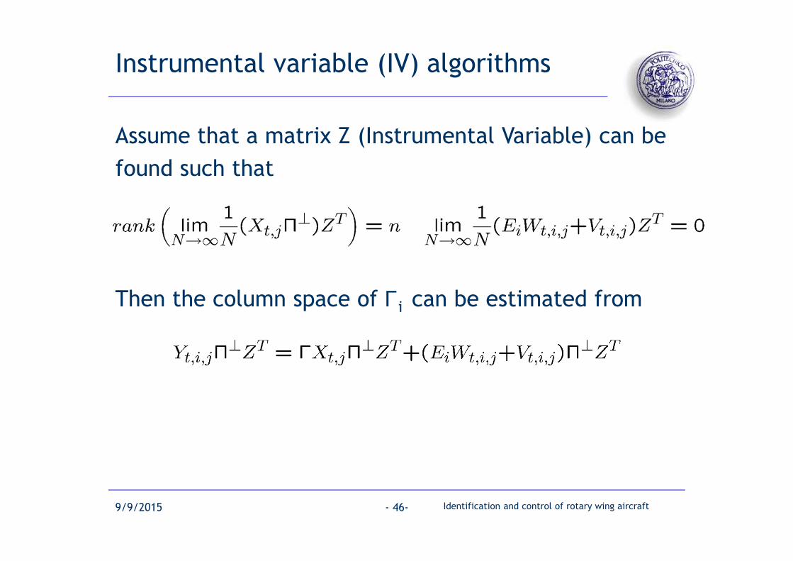
Instrumental variable (IV) algorithms

Assume that a matrix Z (Instrumental Variable) can be

found such that

Then the column space of Γi can be estimated from


The term Yt,i,jΠ?ZT can be computed from the RQ

factorisation

And it holds that

and therefore

Implementation issues


How to choose the IVs

Possible choice of IVs (MOESP-PO, Verhaegen 1994):

Consider the available I/O data set and split it in two parts (past and future), the second shifted ahead of i samples with respect to the first;

Write two separate data equations for past and future data:

Use past data as IVs in the future data equation;


Implementation issues

Using Past Inputs and Outputs as IVs one can compute the RQ factorisation

Rank reduction of estimated column space of Γi

performed via a singular value decomposition.


Persistency of excitation conditions

An input u which is p.e. of order n+2i will “almost

always” lead to a consistent estimate of A and C.

The theory for the IV algorithm is not complete yet…


MATLAB code for the estimation of A and C

function [A,C]=moesppo(u,y,i,j,n);

sy=size(y);su=size(u); datalen=min([max(sy) max(su)]); m=min(su); l=min(sy); Up=[];Uf=[];Yp=[];Yf=[];

for ii=1:i Up=[Up u(ii:ii+j1,:)]; Yp=[Yp y(ii:ii+j1,:)];

end

for ii=i+1:2*i Uf=[Uf u(ii:ii+j1,:)]; Yf=[Yf y(ii:ii+j1,:)];

end

R=triu(qr([Uf Up Yp Yf]))';

R4243=R((2*m+l)*i+1:2*(m+l)*i,m*i+1:(2*m+l)*i);

[U,S,Vt]=svd(R4243);

Un=U(:,1:n);

C=Un(1:l,:);

A=Un(1:l*(i1),:)``Un(l+1:l*i,:);


(Some) extensions of SMI algorithms

Recursive versions of all the presented algorithms;

Identification of linear models in continuous time:

Identification of classes of nonlinear models, including, e.g., Wiener models:

LTIu m y

y=f(m)


Other (important) topics

Choice of parameter i:

The choice of i affects the variance of the estimates;

No general guidelines except for condition i >> n;

Asymptotic variance of the estimated [A,B,C,D] matrices:

Analytical expressions for the variance of the estimates exist;

Expressions too complicated to be of practical use!

The estimates are asymptotically Gaussian;

No results available for efficiency;


SMI vs Prediction Error Methods

Advantages:

SMI algorithms work equally well for SISO and MIMO problems;

They are very reliable from the numerical point of view;

Disadvantages:

SMI algorithms are not “optimal” in any sense;

Very difficult to use them for structured problems;


Available software tools

Functions for SMI in the System Identification Toolbox for Matlab;

Dedicated SMI Toolbox, again based on Matlab;

Fast code in C and Fortran available in the Slicot library.

Documents

Identification of MIMO linear models: introduction to subspace methods · 2017-11-20 · Identification of MIMO linear models: introduction to subspace methods Marco Lovera Dipartimento