Embed Size (px)
Citation preview
S1
Supporting Information
Identification of High Performance Solvents for the
Sustainable Processing of Graphene
Horacio J. Salavagione1, James Sherwood2, Mario De bruyn2, Vitaliy L. Budarin2, Gary Ellis1, James H. Clark2*, Peter S. Shuttleworth1*
1 Departamento de Física de Polímeros, Elastómeros y Aplicaciones Energéticas, Instituto de Ciencia y Tecnología de Polímeros, CSIC, c/ Juan de la Cierva, 3, 28006, Madrid (Spain). 2 Green Chemistry Centre of Excellence, University of York, Heslington, York, Yorkshire, YO10 5DD (UK). e-mail: [email protected]
Electronic Supplementary Material (ESI) for Green Chemistry.This journal is © The Royal Society of Chemistry 2017
S2
Experimental
Materials. Graphite powder with a particle size of 45 µm was purchased from Aldrich (<45
micron, 99.99%, B.N. 496596-113.4G). CVD-graphene on Si covered with a SiO2 layer of 90
nm was purchased from Graphenea, Spain. Triacetin and N-methyl-2-pyrrolidinone (NMP)
were purchased from Sigma Aldrich. Dihydrolevoglucosenone (Cyrene) was obtained from
Circa Group Pty Ltd, and later further purified by first passing the solvent through an alumina
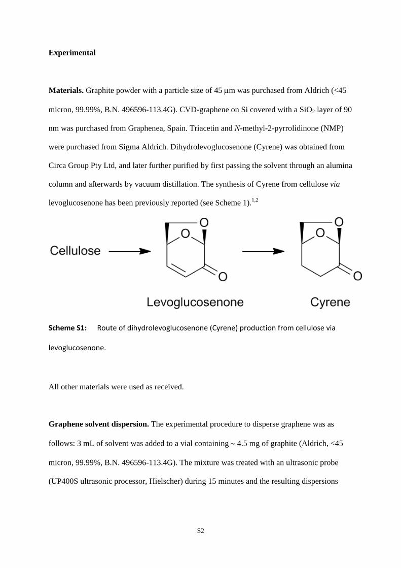
column and afterwards by vacuum distillation. The synthesis of Cyrene from cellulose via
levoglucosenone has been previously reported (see Scheme 1).1,2
Scheme S1: Route of dihydrolevoglucosenone (Cyrene) production from cellulose via
levoglucosenone.
All other materials were used as received.
Graphene solvent dispersion. The experimental procedure to disperse graphene was as
follows: 3 mL of solvent was added to a vial containing ∼ 4.5 mg of graphite (Aldrich, <45
micron, 99.99%, B.N. 496596-113.4G). The mixture was treated with an ultrasonic probe
(UP400S ultrasonic processor, Hielscher) during 15 minutes and the resulting dispersions
S3
were centrifuged at 7000 rpm for 10 minutes. The supernatant after centrifugation was
transferred to a new vial by pipette.
Solvent dispersion concentration. UV-Vis absorption spectra of dispersed graphene in the
solvents NMP, Cyrene, and triacetin were recorded on a Perkin Elmer Lambda 35
spectrophotometer and analysed using the dedicated Perkin Elmer UV Winlab v. 2.85.04
software, with the absorption spectrum shown in Figure S1.
For the UV calibration, 1 mL of centrifuged sample of graphene in Cyrene was passed
through a fluoroporeTM membrane (0.2 µm pore size) and the solid residue carefully weighed,
accounting for any residual solvent to determine the actual dispersion of graphene. The same
solution was diluted several times in order to prepare samples with different graphene
concentrations. Using the UV absorbance at 660 nm,3 where the spectra of the NMP and
Cyrene dispersions both have a gradient of approximately zero, the observed magnitudes of
absorbance were recorded. The variation of absorbance divided by cell length, as a function
of the concentration of graphene dispersed in the reference solutions of Cyrene were plotted
(see Figure 1c, main text) and the line of best fit used to calculate the molar absorptivity
coefficient according to the Lambert-Beer law.
Contact angle. A computer controlled microscope Intel QX3 was used to measure the
contact angle of the tested solvents. CVD-Graphene (on Si/SiO2) pieces (Graphenea),4 were
placed on a manually controlled tilt table with a white light source to illuminate the sample
from behind. With the microscope in the horizontal position, the shape of the static drops of
the different solvents (3 μL) on the surface using a 60x objective were recorded at room
temperature and pressure, and the contact angles calculated using a conventional drop shape
analysis technique (Attension Theta optical tensiometer). Please also refer to Figure S3.

S4
Solvent polarity. The calculation of Hansen solubility parameters and Hansen radii was
performed with the HSPiP software package (4th Edition 4.1.04, developed by Abbott,
Hansen and Yamamoto).
High resolution transmission electron microscopy (TEM). Both Cyrene and NMP
dispersions were analysed using two types of TEM at the Centro Nacional de Microscopía
Electrónica, Madrid, Spain with the aid of a technician, with TEM micrographs taken at
random locations across the grids, to ensure a non-biased assessment. For measurement of
graphene flake lateral dimensions, High-resolution HRTEM micrographs were performed on
a JEOL JEM-2100 instrument (JEOL Ltd., Akishima, Tokyo, Japan), using a LaB6 filament,
a lattice resolution of 0.25 nm and an acceleration voltage of 200 kV. For analysis of the
graphene flake layers and molecular integrity of the graphene flakes, measurements were
carried out on a High-resolution HRTEM micrographs were performed on a JEOL JEM-
3000F instrument (JEOL Ltd., Akishima, Tokyo, Japan), using a LaB6 filament, a lattice
resolution of 0.17 nm and an acceleration voltage of 300 kV. Directly after sonication and
centrifugation the dispersion was added to an equal volume of acetone to dilute it as it was
found that it was too concentrated to achieve a good TEM image, and secondly to aid
evaporation of the solvent. Samples were prepared by drop-casting a few millilitres of
dispersion onto holey carbon films (copper grids) and dried at 120 ºC under vacuum for 12
hours.
Raman spectroscopy characterisation. Raman measurements were undertaken in the
Raman Microspectroscopy Laboratory of the Characterisation Service in the Institute of
Polymer Science & Technology, CSIC using a Renishaw InVia-Reflex Raman system
(Renishaw plc, Wotton-under-Edge, UK), which employed a grating spectrometer with a
Peltier-cooled CCD detector coupled to a confocal microscope. The Raman scattering was
excited with an argon ion laser (λ= 514.5 nm), focusing on the sample with a 100x
S5
microscope objective (NA=0.85) with a laser power of approximately 2 mW at the sample.
Spectra were recorded in the range between 1000 and 3200 cm-1. All spectral data was
processed with Renishaw WiRE 3.2 software. We would like to thank Ms. Isabel Muñoz
Ochando from the Instituto de Ciencia y Tecnología de Polímeros de Madrid (ICTP), CSIC
for help testing the samples.
Additional results
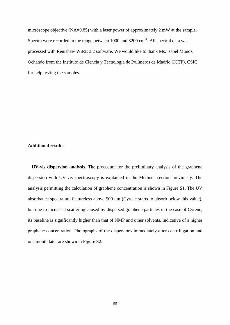
UV-vis dispersion analysis. The procedure for the preliminary analysis of the graphene
dispersion with UV-vis spectroscopy is explained in the Methods section previously. The
analysis permitting the calculation of graphene concentration is shown in Figure S1. The UV
absorbance spectra are featureless above 500 nm (Cyrene starts to absorb below this value),
but due to increased scattering caused by dispersed graphene particles in the case of Cyrene,
its baseline is significantly higher than that of NMP and other solvents, indicative of a higher
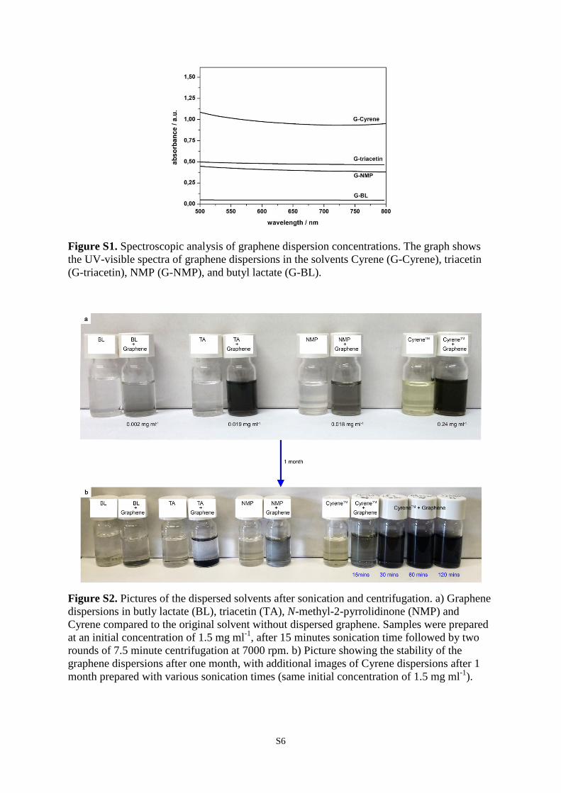
graphene concentration. Photographs of the dispersions immediately after centrifugation and
one month later are shown in Figure S2.
S6
Figure S1. Spectroscopic analysis of graphene dispersion concentrations. The graph shows the UV-visible spectra of graphene dispersions in the solvents Cyrene (G-Cyrene), triacetin (G-triacetin), NMP (G-NMP), and butyl lactate (G-BL).
Figure S2. Pictures of the dispersed solvents after sonication and centrifugation. a) Graphene dispersions in butly lactate (BL), triacetin (TA), N-methyl-2-pyrrolidinone (NMP) and Cyrene compared to the original solvent without dispersed graphene. Samples were prepared at an initial concentration of 1.5 mg ml-1, after 15 minutes sonication time followed by two rounds of 7.5 minute centrifugation at 7000 rpm. b) Picture showing the stability of the graphene dispersions after one month, with additional images of Cyrene dispersions after 1 month prepared with various sonication times (same initial concentration of 1.5 mg ml-1).
S7
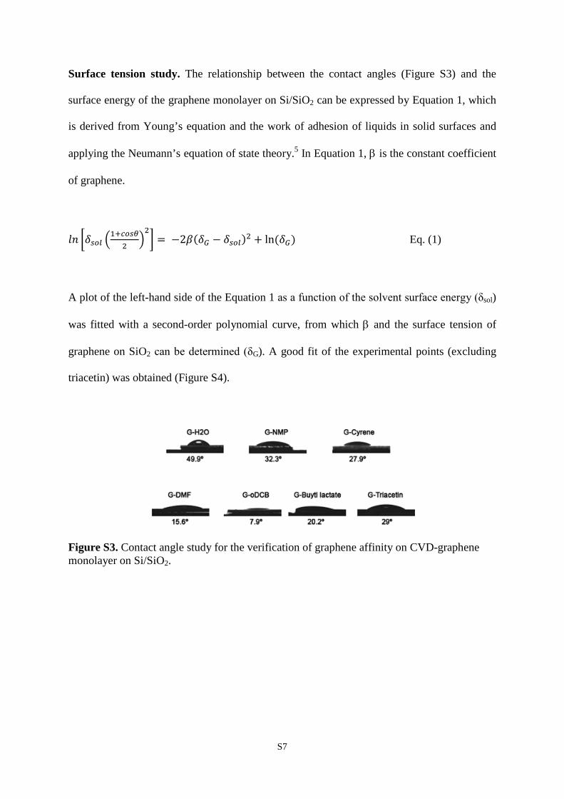
Surface tension study. The relationship between the contact angles (Figure S3) and the
surface energy of the graphene monolayer on Si/SiO2 can be expressed by Equation 1, which
is derived from Young’s equation and the work of adhesion of liquids in solid surfaces and
applying the Neumann’s equation of state theory.5 In Equation 1, β is the constant coefficient
of graphene.
𝑙𝑙 �𝛿𝑠𝑠𝑠 �1+𝑐𝑠𝑠𝑐
2�2� = −2𝛽(𝛿𝐺 − 𝛿𝑠𝑠𝑠)2 + ln (𝛿𝐺) Eq. (1)
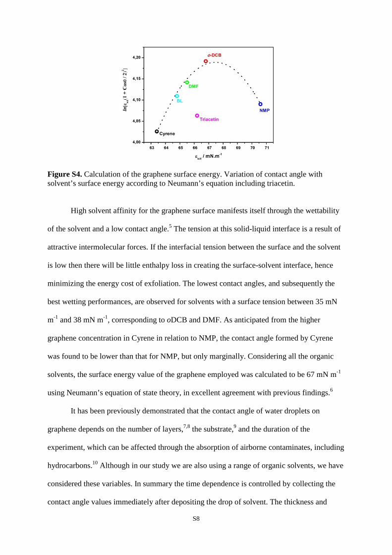
A plot of the left-hand side of the Equation 1 as a function of the solvent surface energy (δsol)
was fitted with a second-order polynomial curve, from which β and the surface tension of
graphene on SiO2 can be determined (δG). A good fit of the experimental points (excluding
triacetin) was obtained (Figure S4).
Figure S3. Contact angle study for the verification of graphene affinity on CVD-graphene monolayer on Si/SiO2.
S8
Figure S4. Calculation of the graphene surface energy. Variation of contact angle with solvent’s surface energy according to Neumann’s equation including triacetin.
High solvent affinity for the graphene surface manifests itself through the wettability
of the solvent and a low contact angle.5 The tension at this solid-liquid interface is a result of
attractive intermolecular forces. If the interfacial tension between the surface and the solvent
is low then there will be little enthalpy loss in creating the surface-solvent interface, hence
minimizing the energy cost of exfoliation. The lowest contact angles, and subsequently the
best wetting performances, are observed for solvents with a surface tension between 35 mN
m-1 and 38 mN m-1, corresponding to oDCB and DMF. As anticipated from the higher
graphene concentration in Cyrene in relation to NMP, the contact angle formed by Cyrene
was found to be lower than that for NMP, but only marginally. Considering all the organic
solvents, the surface energy value of the graphene employed was calculated to be 67 mN m-1
using Neumann’s equation of state theory, in excellent agreement with previous findings.6
It has been previously demonstrated that the contact angle of water droplets on
graphene depends on the number of layers,7,8 the substrate,9 and the duration of the
experiment, which can be affected through the absorption of airborne contaminates, including
hydrocarbons.10 Although in our study we are also using a range of organic solvents, we have
considered these variables. In summary the time dependence is controlled by collecting the
contact angle values immediately after depositing the drop of solvent. The thickness and
S9
uniformity of the CVD-graphene were evaluated by Raman spectroscopy. The I2D/IG intensity
ratio and the full width at half-maximum of the 2D band, related to the number of CVD-
graphene layers, are 1.7 ± 0.2 and 36.9 ± 0.8 cm-1 respectively, resembling the values
previously observed for CVD-graphene.11,12 This data is indicative of graphene uniformly
distributed on the Si/SiO2 surface, allowing us to discard the effect of the graphene thickness
on the contact angles. Moreover, reference experiments of contact angles on Si/SiO2 wafers
(without graphene) were conducted to evaluate the influence of the substrate. The measured
values were very similar for all organic solvents (∼32.0º to 36.6º) demonstrating minimal
influence of the Si/SiO2 substrate on the contact angle.
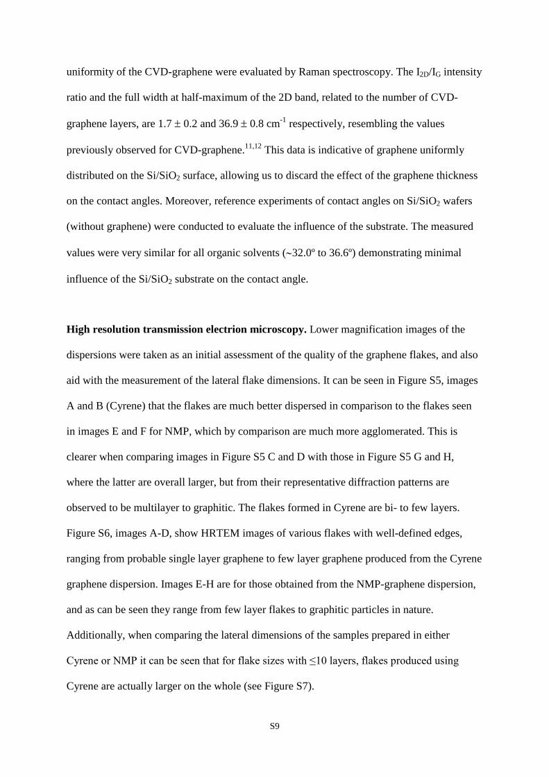
High resolution transmission electrion microscopy. Lower magnification images of the
dispersions were taken as an initial assessment of the quality of the graphene flakes, and also
aid with the measurement of the lateral flake dimensions. It can be seen in Figure S5, images
A and B (Cyrene) that the flakes are much better dispersed in comparison to the flakes seen
in images E and F for NMP, which by comparison are much more agglomerated. This is
clearer when comparing images in Figure S5 C and D with those in Figure S5 G and H,
where the latter are overall larger, but from their representative diffraction patterns are
observed to be multilayer to graphitic. The flakes formed in Cyrene are bi- to few layers.
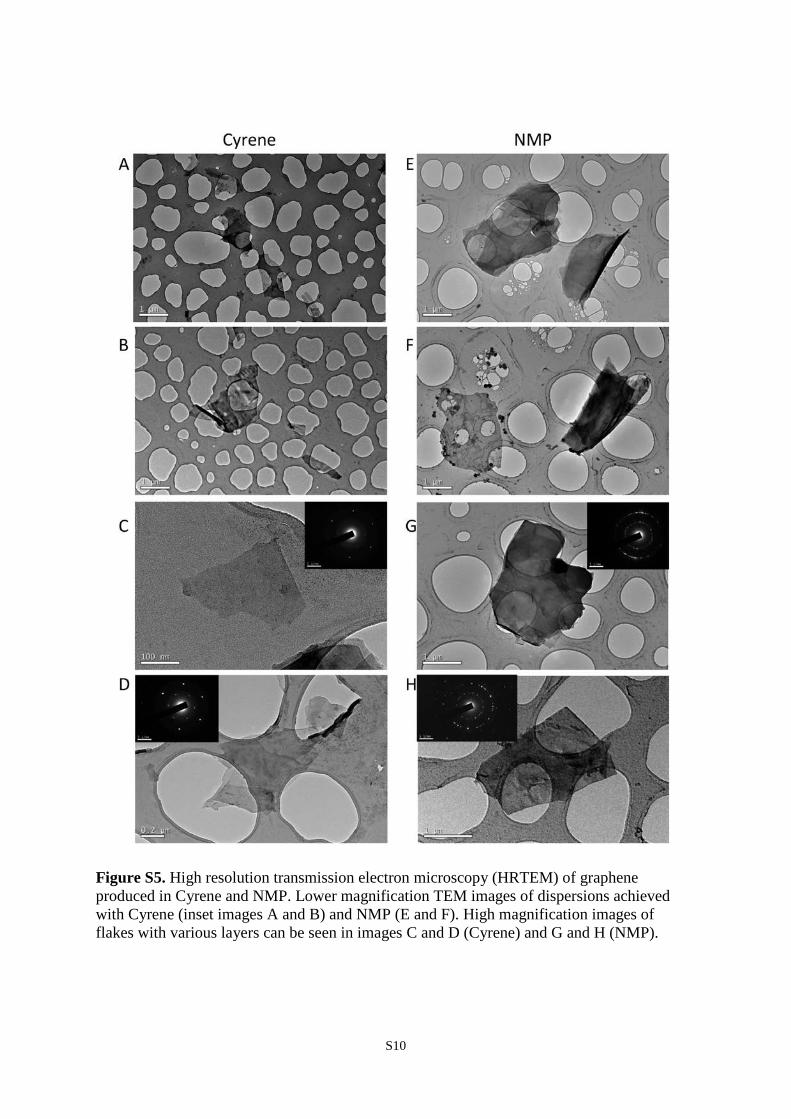
Figure S6, images A-D, show HRTEM images of various flakes with well-defined edges,
ranging from probable single layer graphene to few layer graphene produced from the Cyrene
graphene dispersion. Images E-H are for those obtained from the NMP-graphene dispersion,
and as can be seen they range from few layer flakes to graphitic particles in nature.
Additionally, when comparing the lateral dimensions of the samples prepared in either
Cyrene or NMP it can be seen that for flake sizes with ≤10 layers, flakes produced using
Cyrene are actually larger on the whole (see Figure S7).
S10
Figure S5. High resolution transmission electron microscopy (HRTEM) of graphene produced in Cyrene and NMP. Lower magnification TEM images of dispersions achieved with Cyrene (inset images A and B) and NMP (E and F). High magnification images of flakes with various layers can be seen in images C and D (Cyrene) and G and H (NMP).
S11
Figure S6. HRTEM images showing the edges of Cyrene dispersed graphene (inset images A-D) and NMP dispersed graphene (E-H).

S12
Figure S7. Flake length (L) and width (W) dimensions taken from TEM measurements for both Cyrene (left) and NMP (right) dispersions.
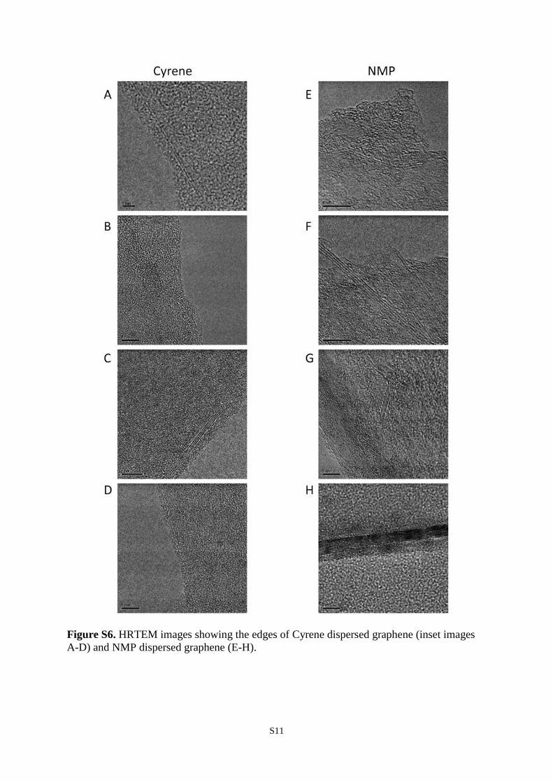
Raman graphene quality analysis. Examination of the Raman 2D band in this work was
found to be very instructive in ruling out whether the postulated ‘protection’ offered by
viscous solvents counteracts the critical role of surface tension. It is accepted that the number
of Lorentzian curves (FWHM ~ 24) making up the 2D band relates to the number of stacked
graphene layers.13-15 Here deconvolution of 2D Raman band for Cyrene suggested the
formation of polydisperse samples ranging from two to a few and multilayers graphene,
similar to NMP treated under the same conditions (Figure S8). Furthermore, the 2D band
width, another parameter used to determine the thickness of graphene laminates, is very
similar for both samples, which also suggests that they represent a similar thickness of
graphene.16 The difference between this and the results of TEM etc. are due to the extended
drying times of the dispersion on the Si/SiO2 wafer in comparison to the holey carbon grid
used for TEM and also the fact that monolayer graphene is virtually invisible under an optical
S13
microscope to be able to locate them and test them, even when using recommended Si/SiO2
(300 nm).
Figure S8. Raman 2D band deconvolution to estimate the number of graphene stacked layers. The spectra were acquired in different points of samples deposited by drop-casting on Si/SiO2 substrates.
A general expression to estimate the crystallite size La from the integrated intensity
ratio ID/ IG has been proposed by Cançado et al.,17 and can be written as follows (Equation 2)
where λ is the laser wavelength in nm, in this case 514 nm.
𝐿𝑎(𝑙𝑛) = 2.4𝑥10−10𝜆𝑠4(𝐼𝐷𝐼𝐺
)−1 Eq. (2)

S14
The distance between defects (LD) and the defect density (nD) can also be estimated from the
ID/ IG using experimentally determined equations.18 The LD can be written as is shown in
Equation 3, and the density of defect as Equation 4.
𝐿𝐷2 (𝑙𝑛2) = (1.8 ± 0.5) × 10−9𝜆𝑠4 �𝐼𝐷𝐼𝐺�−1
Eq. (3)
𝑙𝐷(𝑐𝑛−2) = (1.8±0.5)×1022
𝜆𝑙4 �𝐼𝐷
𝐼𝐺� Eq. (4)
Changes in La, LD, and the defect density (nD) compared with the viscosity of the
tested solvents are shown in Figure S9.
S15
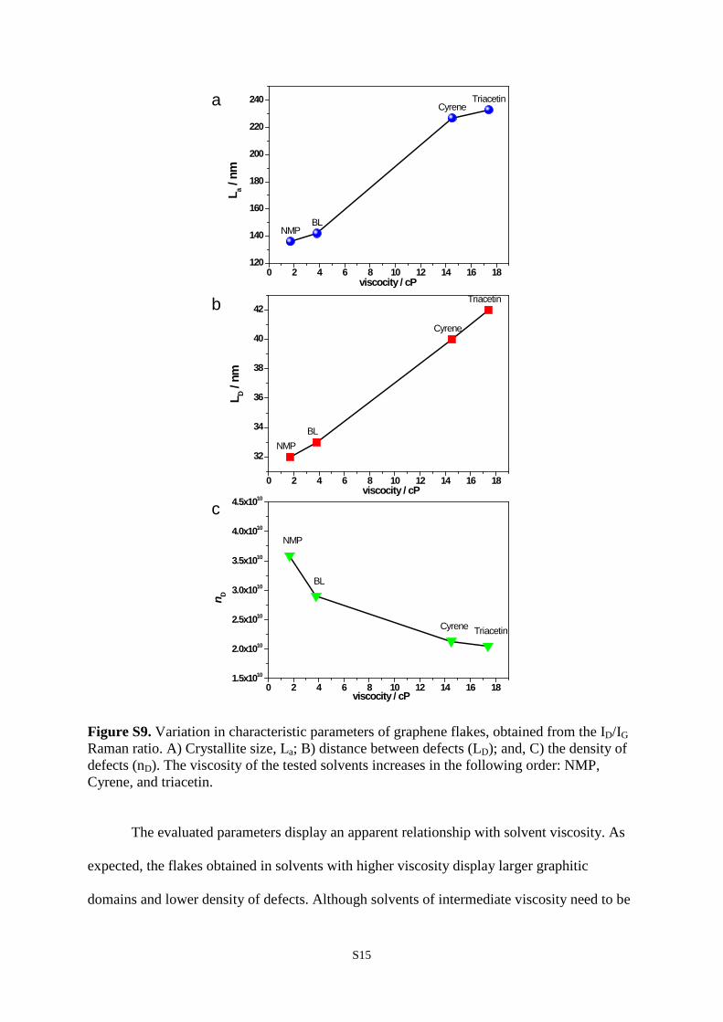
Figure S9. Variation in characteristic parameters of graphene flakes, obtained from the ID/IG Raman ratio. A) Crystallite size, La; B) distance between defects (LD); and, C) the density of defects (nD). The viscosity of the tested solvents increases in the following order: NMP, Cyrene, and triacetin.
The evaluated parameters display an apparent relationship with solvent viscosity. As
expected, the flakes obtained in solvents with higher viscosity display larger graphitic
domains and lower density of defects. Although solvents of intermediate viscosity need to be
0 2 4 6 8 10 12 14 16 181.5x10¹⁰
2.0x10¹⁰
2.5x10¹⁰
3.0x10¹⁰
3.5x10¹⁰
4.0x10¹⁰
4.5x10¹⁰
NMP
BL
Cyrene Triacetin
viscocity / cP
n D
0 2 4 6 8 10 12 14 16 18
32
34
36
38
40
42
NMPBL
Cyrene
Triacetin
L D / n
m
viscocity / cP
0 2 4 6 8 10 12 14 16 18120
140
160
180
200
220
240
NMPBL
CyreneTriacetin
L a / n
m
viscocity / cP
a
b
c

S16
tested to appropriately obtain an equation describing the variation of each parameter with
viscosity, the data in Figure S9 clearly demonstrates the effect of viscosity on the structural
integrity of graphene flakes.
Exfoliation optimization. The experimental parameters, e.g. sonication time and initial
graphite concentration that determine the concentration of the dispersed graphene were re-
evaluated. Long sonication times have previously been reported as a means to obtain high
graphene concentrations in NMP.19 This this may also be advantageous for dispersions in
Cyrene. The aim of our investigation here was to establish the optimal conditions that
maximize the dispersion of graphene for commercially pertinent applications, whilst
preserving the structural integrity of the graphene flakes.
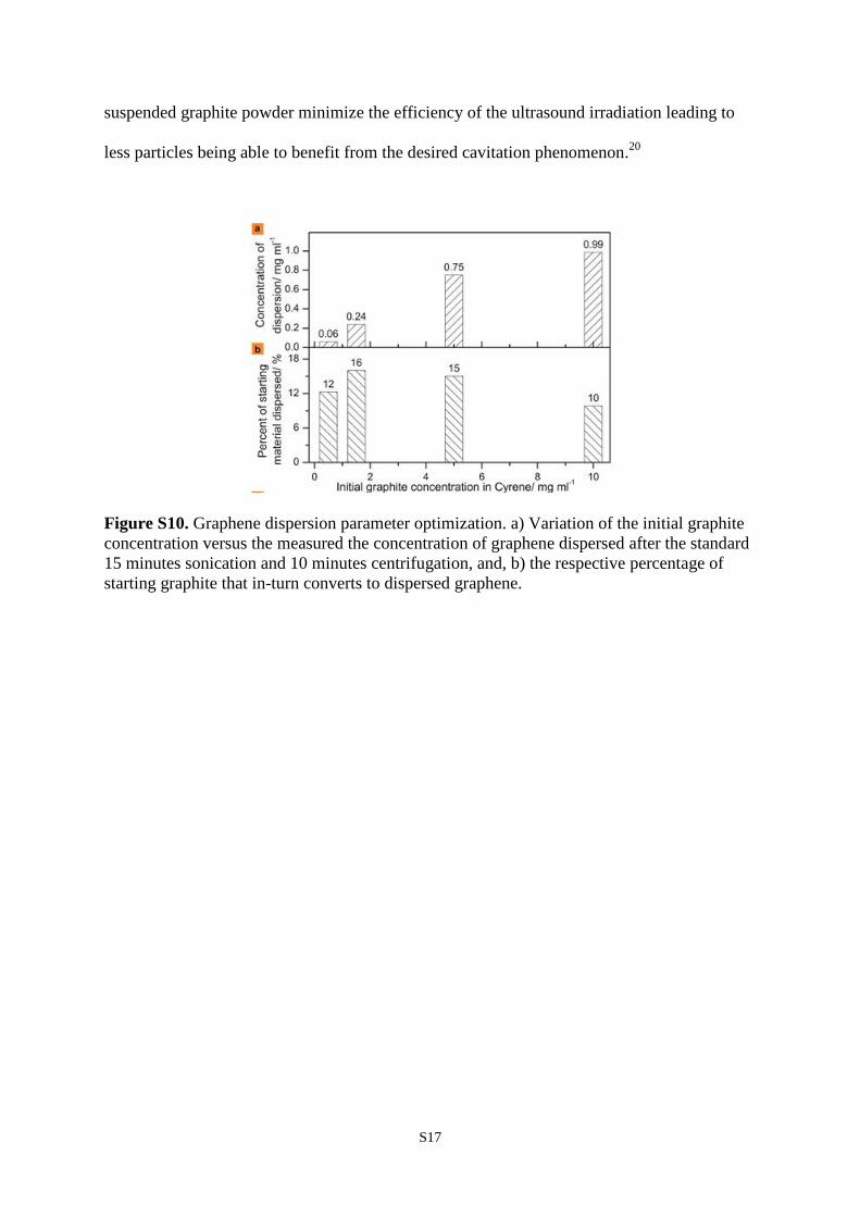
Firstly, different initial concentrations of graphite, Ci, of 0.5, 1.5, 5.0 and 10 mg mL-1
were tested to evaluate the exfoliation of graphite to dispersed graphene in Cyrene (Figure
S10a). The amount of dispersed material was determined by UV-visible spectroscopy, where
the absorbance at 660 nm was measured in the same way as previously outlined. An almost
linear dependence of the amount of dispersed graphene versus the starting graphite amount
was observed up to Ci = 5 mg mL-1, with the gradient accounting for an additional 0.15 mg of
dispersed particles for every 1 mg increase in the starting graphite loading. Few gains are
made beyond an initial graphite concentration of 5 mg mL-1, but still graphene concentrations
of ~1 mg mL-1 can be reached with an initial graphite load of Ci = 10 mg mL-1. Figure S10b
presents the percentage of the initial graphite that can be converted into dispersed particles. It
is evident that this quantity initially increases, reaching a maximum (16%) in the range 1.5
mg mL-1 < Ci < 5 mg mL-1 and then decreases significantly to no more than 10% when Ci =
10 mg mL-1. This trend can be related to the effect of powdered graphite particles on the
efficiency of sonication, and consequently exfoliation. Specifically, high amounts of
S17
suspended graphite powder minimize the efficiency of the ultrasound irradiation leading to
less particles being able to benefit from the desired cavitation phenomenon.20
Figure S10. Graphene dispersion parameter optimization. a) Variation of the initial graphite concentration versus the measured the concentration of graphene dispersed after the standard 15 minutes sonication and 10 minutes centrifugation, and, b) the respective percentage of starting graphite that in-turn converts to dispersed graphene.
S18
Solvent selection procedure
Overview. A solvent selection protocol was developed to identify ideal solvents for graphene
processing and to help define the precise role of the solvent. Given the clearly recognisable
need, the methodology was developed to find a high performance yet green solvent.
Algorithms for solvent selection have been used previously to optimise the solvent for simple
extractions, and in examples of reaction chemistry.21 If the requirements of the solvent can be
defined in terms of measurable properties, then we postulated that the principle can also be
applied to the more complex problem of graphite exfoliation and the subsequent dispersion of
graphene flakes in solution. There has been much debate over the exact role of the solvent in
the processing of carbon nanostructures,22-25 which is not fully understood. Nevertheless there
is a consensus that solvent surface energy and viscosity are both crucially important in order
to achieve an acceptable concentration of dispersed graphene.3,25 The polarity of the medium
is also influential, and Hansen solubility parameters have been used previously to correlate
graphene concentration to solvent polarity.26,27 However different reports do not always agree
on the significance of each solvent property, or in some instances what the ideal value of that
property actually is.3,5 That being the case, an approach to solvent selection that can be easily
updated, added to, or otherwise modified is greatly beneficial.
Here we report a high throughput screening of a large database of solvents in order to
identify green solvents able to disperse graphene in relatively high concentrations. After a
comprehensive selection process, the most promising solvent candidates, as indicated through
calculation, were subjected to an experimental validation of their performance. This multi-
stage assessment of solvent properties was designed to refine a large solvent dataset, far
beyond the number of solvents that could actually be tested experimentally, to only the
environmentally friendly solvent candidates with an anticipated high performance. This is a
S19
key difference between this approach and the solely experimental methods of other studies
that make use of Hansen solubility parameters.26 A series of experiments and analysis
confirmed the theoretical predictions, with Cyrene for example achieving highly concentrated
dispersions of quality graphene flakes.
To the best of the authors’ knowledge, this work is the first attempt to select a solvent
for creating graphene dispersions by considering relevant properties in a logical, systematic
way, but crucially without the restriction of choosing a solvent from a small experimental set.
The approach employed reduces a large number of possible solvent candidates to a shortlist
consisting of only those solvents that meet the requirements of each criterion. Thus,
experimental validation of the solvent selection protocol is only required for a minimal
number of solvents, thus creating a streamlined investigation that at the same time actually
encompasses several hundreds of solvents more than a typical, experimentally led project.
The act of carrying out the solvent selection process creates a better understanding of the
relevant solvent characteristics. This in turn assists with future solvent development, where
the solvent selection process may be adapted or new solvent candidates introduced in later
iterations. A concise version of the assessment is provided as a separate (Microsoft Excel)
file.
The first round of the methodology concerns the solvent properties that influence the
performance of the process (i.e. ultrasound assisted exfoliation and graphene dispersion). A
polarity matching exercise using Hansen solubility parameters established suitable solvents
on the basis of bulk solution interactions with graphene. Target parameters representing the
polarity of graphene were obtained from the literature.26 Secondly the interaction between the
solvent and graphene through their surface energies, again relevant to exfoliation and
dispersion stability, was also used to select promising solvent candidates.5,6 Finally the
stability of a graphene suspension was approximated using Stokes’ law of settling velocities,

S20
where the density/viscosity ratio is important (as explained subsequently). The three criteria
were applied in individual assessments, not sequentially (Table S1). This is so that if a
requirement is changed, the recalculation of the solvent shortlist is simplified. Solvent
candidates move through to the next stage of the assessment only if they meet the
requirements of all three parallel performance criteria.
Table S1. Solvent selection performance criteria.
Performance metric
Measurement Target Requirement
Solvent-solute interaction
Polarity (calculated) δD = 18 MPa0.5
δP = 9.3 MPa0.5
δH = 7.7 MPa0.5
Hansen distance between target and solvent lower than 6.5 MPa0.5.
Solvent-solute interaction
Surface tension γ = 38.2 ± 6
mN·m-1
Solvent surface tension falls within designated range.
Dispersion stability
Density (ρ /g·mL-1) and dynamic viscosity (μ / g·s-1·m-1)
ρ/μ ≤ 1.20 106 s·m-2
Low density/viscosity ratio.
The original dataset of solvents exceeded 10,000 entries. The large number of solvent
candidates was processed using the HSPiP solubility estimation software package, sorting by
polarity. The remaining data analysis was performed in a spreadsheet (refer to the separate
electronic supplementary information file). Many of the solvents contained in the dataset lack
experimental viscosity and surface tension data, meaning they cannot pass all the solvent
selection criteria for this reason alone. However this exercise does highlight promising
solvents that could be synthesised and their additional physical properties tested.
Computational estimates could also guide this task and future work will investigate this
possibility further. The original HSPiP dataset from which the list of solvent candidates was
derived was supplemented by a number of bio-based solvents, to which special interest was
S21
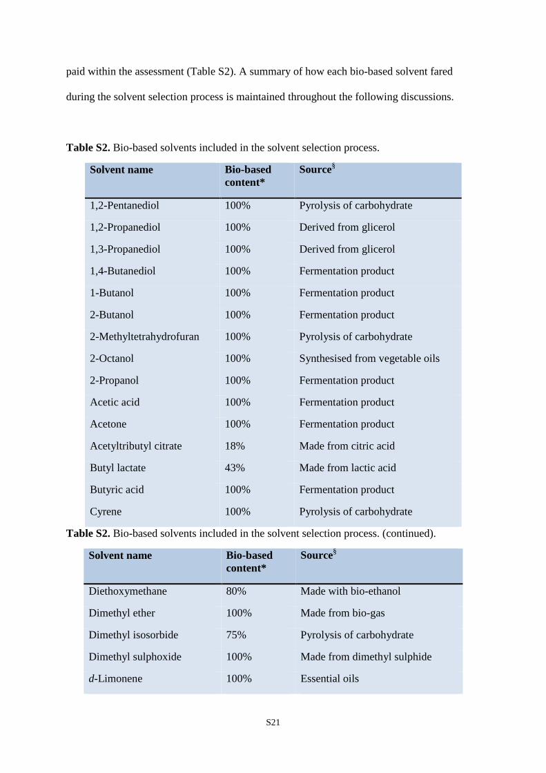
paid within the assessment (Table S2). A summary of how each bio-based solvent fared
during the solvent selection process is maintained throughout the following discussions.
Table S2. Bio-based solvents included in the solvent selection process.
Solvent name Bio-based content*
Source§
1,2-Pentanediol 100% Pyrolysis of carbohydrate
1,2-Propanediol 100% Derived from glicerol
1,3-Propanediol 100% Derived from glicerol
1,4-Butanediol 100% Fermentation product
1-Butanol 100% Fermentation product
2-Butanol 100% Fermentation product
2-Methyltetrahydrofuran 100% Pyrolysis of carbohydrate
2-Octanol 100% Synthesised from vegetable oils
2-Propanol 100% Fermentation product
Acetic acid 100% Fermentation product
Acetone 100% Fermentation product
Acetyltributyl citrate 18% Made from citric acid
Butyl lactate 43% Made from lactic acid
Butyric acid 100% Fermentation product
Cyrene 100% Pyrolysis of carbohydrate
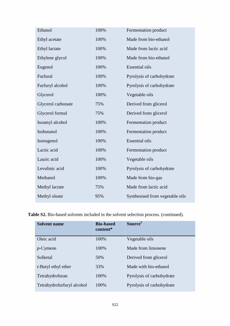
Table S2. Bio-based solvents included in the solvent selection process. (continued).
Solvent name Bio-based content*
Source§
Diethoxymethane 80% Made with bio-ethanol
Dimethyl ether 100% Made from bio-gas
Dimethyl isosorbide 75% Pyrolysis of carbohydrate
Dimethyl sulphoxide 100% Made from dimethyl sulphide
d-Limonene 100% Essential oils
S22
Ethanol 100% Fermentation product
Ethyl acetate 100% Made from bio-ethanol
Ethyl lactate 100% Made from lactic acid
Ethylene glycol 100% Made from bio-ethanol
Eugenol 100% Essential oils
Furfural 100% Pyrolysis of carbohydrate
Furfuryl alcohol 100% Pyrolysis of carbohydrate
Glycerol 100% Vegetable oils
Glycerol carbonate 75% Derived from glicerol
Glycerol formal 75% Derived from glicerol
Isoamyl alcohol 100% Fermentation product
Isobutanol 100% Fermentation product
Isoeugenol 100% Essential oils
Lactic acid 100% Fermentation product
Lauric acid 100% Vegetable oils
Levulinic acid 100% Pyrolysis of carbohydrate
Methanol 100% Made from bio-gas
Methyl lactate 75% Made from lactic acid
Methyl oleate 95% Synthesised from vegetable oils
Table S2. Bio-based solvents included in the solvent selection process. (continued).
Solvent name Bio-based content*
Source§
Oleic acid 100% Vegetable oils
p-Cymene 100% Made from limonene
Solketal 50% Derived from glicerol
t-Butyl ethyl ether 33% Made with bio-ethanol
Tetrahydrofuran 100% Pyrolysis of carbohydrate
Tetrahydrofurfuryl alcohol 100% Pyrolysis of carbohydrate
S23
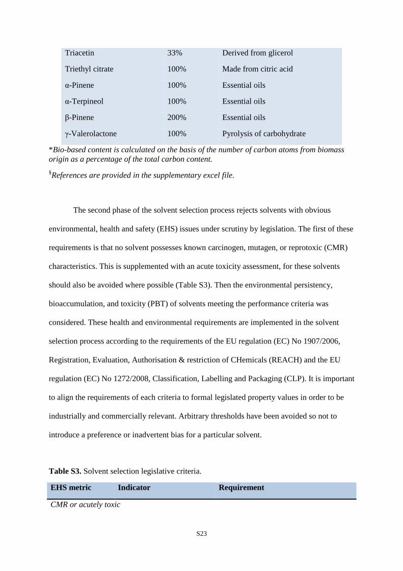
Triacetin 33% Derived from glicerol
Triethyl citrate 100% Made from citric acid
α-Pinene 100% Essential oils
α-Terpineol 100% Essential oils
β-Pinene 200% Essential oils
γ-Valerolactone 100% Pyrolysis of carbohydrate
*Bio-based content is calculated on the basis of the number of carbon atoms from biomass origin as a percentage of the total carbon content. §References are provided in the supplementary excel file.
The second phase of the solvent selection process rejects solvents with obvious
environmental, health and safety (EHS) issues under scrutiny by legislation. The first of these
requirements is that no solvent possesses known carcinogen, mutagen, or reprotoxic (CMR)
characteristics. This is supplemented with an acute toxicity assessment, for these solvents
should also be avoided where possible (Table S3). Then the environmental persistency,
bioaccumulation, and toxicity (PBT) of solvents meeting the performance criteria was
considered. These health and environmental requirements are implemented in the solvent
selection process according to the requirements of the EU regulation (EC) No 1907/2006,
Registration, Evaluation, Authorisation & restriction of CHemicals (REACH) and the EU
regulation (EC) No 1272/2008, Classification, Labelling and Packaging (CLP). It is important
to align the requirements of each criteria to formal legislated property values in order to be
industrially and commercially relevant. Arbitrary thresholds have been avoided so not to
introduce a preference or inadvertent bias for a particular solvent.
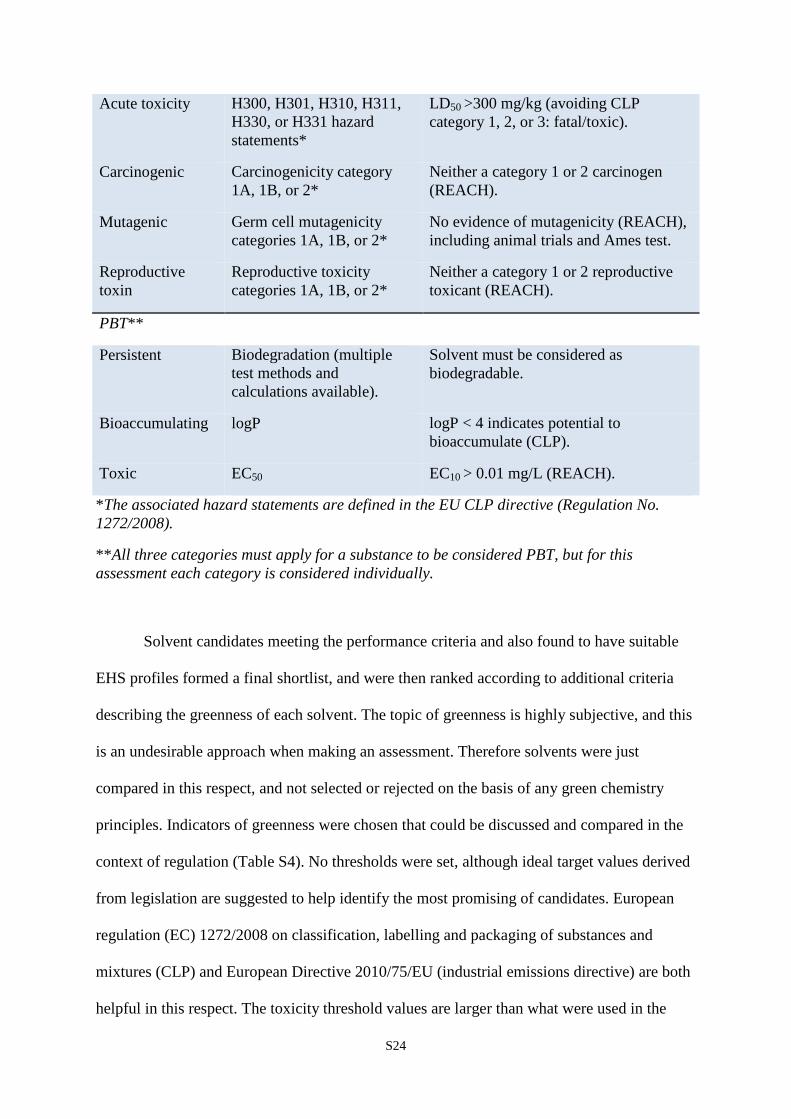
Table S3. Solvent selection legislative criteria.
EHS metric Indicator Requirement
CMR or acutely toxic
S24
Acute toxicity H300, H301, H310, H311, H330, or H331 hazard statements*
LD50 >300 mg/kg (avoiding CLP category 1, 2, or 3: fatal/toxic).
Carcinogenic Carcinogenicity category 1A, 1B, or 2*
Neither a category 1 or 2 carcinogen (REACH).
Mutagenic Germ cell mutagenicity categories 1A, 1B, or 2*
No evidence of mutagenicity (REACH), including animal trials and Ames test.
Reproductive toxin
Reproductive toxicity categories 1A, 1B, or 2*
Neither a category 1 or 2 reproductive toxicant (REACH).
PBT**
Persistent Biodegradation (multiple test methods and calculations available).
Solvent must be considered as biodegradable.
Bioaccumulating logP logP < 4 indicates potential to bioaccumulate (CLP).
Toxic EC50 EC10 > 0.01 mg/L (REACH).
*The associated hazard statements are defined in the EU CLP directive (Regulation No. 1272/2008).
**All three categories must apply for a substance to be considered PBT, but for this assessment each category is considered individually.
Solvent candidates meeting the performance criteria and also found to have suitable
EHS profiles formed a final shortlist, and were then ranked according to additional criteria
describing the greenness of each solvent. The topic of greenness is highly subjective, and this
is an undesirable approach when making an assessment. Therefore solvents were just
compared in this respect, and not selected or rejected on the basis of any green chemistry
principles. Indicators of greenness were chosen that could be discussed and compared in the
context of regulation (Table S4). No thresholds were set, although ideal target values derived
from legislation are suggested to help identify the most promising of candidates. European
regulation (EC) 1272/2008 on classification, labelling and packaging of substances and
mixtures (CLP) and European Directive 2010/75/EU (industrial emissions directive) are both
helpful in this respect. The toxicity threshold values are larger than what were used in the

S25
EHS criteria, broadened out to include less severe hazards, yet still requiring labelling
according to the CLP directive. In addition, bio-based solvents made from renewable
resources were prioritised, under the guidance of European Technical Specification
TS/16766.28 This process helped to identify butyl lactate, Cyrene, and triacetin as the primary
candidates for the sustainable solvent processing of graphene, incorporating practical,
regulatory, environmental, health, and safety aspects as part of this judgement. Greater detail
on each of these assessment phases is now provided. A spreadsheet containing the solvent
selection calculations has also been made available for greater detail.
S26
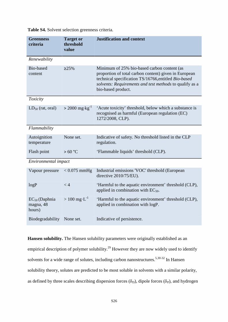
Table S4. Solvent selection greenness criteria.
Greenness criteria
Target or threshold value
Justification and context
Renewability
Bio-based content
≥25% Minimum of 25% bio-based carbon content (as proportion of total carbon content) given in European technical specification TS/16766,entitled Bio-based solvents: Requirements and test methods to qualify as a bio-based product.
Toxicity
LD50 (rat, oral) > 2000 mg·kg-1 ‘Acute toxicity’ threshold, below which a substance is recognised as harmful (European regulation (EC) 1272/2008, CLP).
Flammability
Autoignition temperature
None set. Indicative of safety. No threshold listed in the CLP regulation.
Flash point > 60 °C ‘Flammable liquids’ threshold (CLP).
Environmental impact
Vapour pressure < 0.075 mmHg Industrial emissions 'VOC' threshold (European directive 2010/75/EU).
logP < 4 ‘Harmful to the aquatic environment’ threshold (CLP), applied in combination with EC50.
EC50 (Daphnia magna, 48 hours)
> 100 mg·L-1 ‘Harmful to the aquatic environment’ threshold (CLP), applied in combination with logP.
Biodegradability None set. Indicative of persistence.
Hansen solubility. The Hansen solubility parameters were originally established as an
empirical description of polymer solubility.29 However they are now widely used to identify
solvents for a wide range of solutes, including carbon nanostructures.5,30-32 In Hansen
solubility theory, solutes are predicted to be most soluble in solvents with a similar polarity,
as defined by three scales describing dispersion forces (δD), dipole forces (δP), and hydrogen

S27
bonding interactions (δH). The length of a vector connecting a solvent to a solute in this three
dimensional Hansen space is indicative of the likely solubility. Using characteristic values for
graphene (δD ∼ 18.0 MPa1/2; δP ∼ 9.3 MPa1/2; δH ∼ 7.7 MPa1/2),26 potential solvents can be
found computationally. The Hansen parameters are typically calculated rather than obtained
from experiments, so the potential solvent set is infinite. This equally applies to theoretical
solvent structures before they are first synthesised. Using the Hansen Solubility Parameters
in Practice (HSPiP) software, a number of potential graphene dispersing solvents were
identified from more than 10,000 candidates contained within the software. As stated earlier,
this dataset was complimented with 51 bio-based solvent entries taken from the University of
York’s Sustainable Solvent Selection Service (S4) database.
A representative selection of solvents is shown in the following polarity diagram to
demonstrate the solvent selection process (Figure S11). The assignment of solvents and non-
solvents, and hence the boundary of the so-called solubility sphere (shown in green) was
defined using a minimal number of experimental observations already available in the
literature. While acetone is seen as a poor solvent for graphene dispersibility,26 it is actually a
better polarity match to graphene in the 3D Hansen space (radius of 5.2 MPa0.5) than DMF
(5.8 MPa0.5), the latter being a recognised solvent. This suggests other solvent properties are
relevant. A sphere radius of 6.5 MPa0.5 was chosen to differentiate between potentially
suitable and unsuitable solvents on the basis of polarity (Figure S11). Acetone and DMF are
both contained within this boundary.
S28
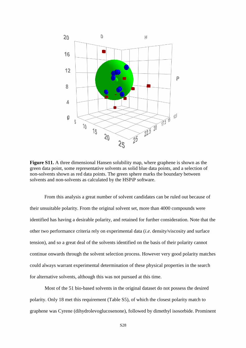
Figure S11. A three dimensional Hansen solubility map, where graphene is shown as the green data point, some representative solvents as solid blue data points, and a selection of non-solvents shown as red data points. The green sphere marks the boundary between solvents and non-solvents as calculated by the HSPiP software.
From this analysis a great number of solvent candidates can be ruled out because of
their unsuitable polarity. From the original solvent set, more than 4000 compounds were
identified has having a desirable polarity, and retained for further consideration. Note that the
other two performance criteria rely on experimental data (i.e. density/viscosity and surface
tension), and so a great deal of the solvents identified on the basis of their polarity cannot
continue onwards through the solvent selection process. However very good polarity matches
could always warrant experimental determination of these physical properties in the search
for alternative solvents, although this was not pursued at this time.
Most of the 51 bio-based solvents in the original dataset do not possess the desired
polarity. Only 18 met this requirement (Table S5), of which the closest polarity match to
graphene was Cyrene (dihydrolevoglucosenone), followed by dimethyl isosorbide. Prominent

S29
bio-based solvents with an undesirable polarity, and thus eliminated from the assessment,
included limonene, ethanol, and glycerol.
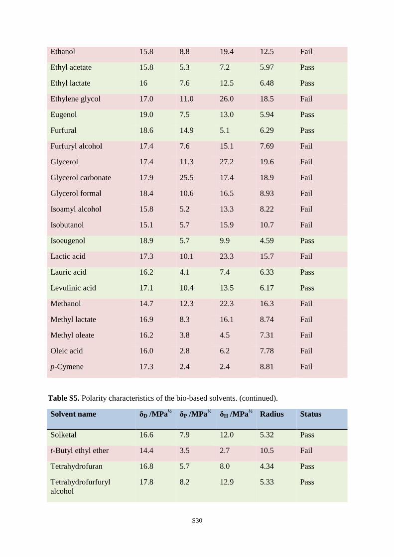
Table S5. Polarity characteristics of the bio-based solvents.
Solvent name δD /MPa½ δP /MPa½ δH /MPa½ Radius Status
1,2-Pentanediol 16.7 7.2 16.8 9.69 Fail
1,2-Propanediol 16.8 10.4 21.3 13.9 Fail
1,3-Propanediol 16.8 13.5 23.2 16.2 Fail
1,4-Butanediol 16.6 11.0 20.9 13.6 Fail
1-Butanol 16.0 5.7 15.8 9.72 Fail
2-Butanol 15.8 5.7 14.5 8.86 Fail
2-Methyltetrahydrofuran 16.9 5.0 4.3 5.91 Pass
2-Octanol 16.1 4.2 9.1 6.51 Fail
2-Propanol 15.8 6.1 16.4 10.3 Fail
Acetic acid 14.5 8.0 13.5 9.18 Fail
Acetone 15.5 10.4 7.0 5.17 Pass
Acetyltributyl citrate 16.7 2.5 7.4 7.29 Fail
Butyl lactate 15.8 6.5 10.2 5.78 Pass
Butyric acid 15.7 4.8 12.0 7.74 Fail
Cyrene 18.8 10.6 6.9 2.21 Pass
Diethoxymethane 15.4 5.7 5.1 6.84 Fail
Table S5. Polarity characteristics of the bio-based solvents. (continued).
Solvent name δD /MPa½ δP /MPa½ δH /MPa½ Radius Status
Dimethyl isosorbide 17.6 7.1 7.5 2.35 Pass
Dimethyl sulphoxide 18.4 16.4 10.2 7.57 Fail
d-Limonene 17.2 1.8 4.3 8.39 Fail
S30
Ethanol 15.8 8.8 19.4 12.5 Fail
Ethyl acetate 15.8 5.3 7.2 5.97 Pass
Ethyl lactate 16 7.6 12.5 6.48 Pass
Ethylene glycol 17.0 11.0 26.0 18.5 Fail
Eugenol 19.0 7.5 13.0 5.94 Pass
Furfural 18.6 14.9 5.1 6.29 Pass
Furfuryl alcohol 17.4 7.6 15.1 7.69 Fail
Glycerol 17.4 11.3 27.2 19.6 Fail
Glycerol carbonate 17.9 25.5 17.4 18.9 Fail
Glycerol formal 18.4 10.6 16.5 8.93 Fail
Isoamyl alcohol 15.8 5.2 13.3 8.22 Fail
Isobutanol 15.1 5.7 15.9 10.7 Fail
Isoeugenol 18.9 5.7 9.9 4.59 Pass
Lactic acid 17.3 10.1 23.3 15.7 Fail
Lauric acid 16.2 4.1 7.4 6.33 Pass
Levulinic acid 17.1 10.4 13.5 6.17 Pass
Methanol 14.7 12.3 22.3 16.3 Fail
Methyl lactate 16.9 8.3 16.1 8.74 Fail
Methyl oleate 16.2 3.8 4.5 7.31 Fail
Oleic acid 16.0 2.8 6.2 7.78 Fail
p-Cymene 17.3 2.4 2.4 8.81 Fail
Table S5. Polarity characteristics of the bio-based solvents. (continued).
Solvent name δD /MPa½ δP /MPa½ δH /MPa½ Radius Status
Solketal 16.6 7.9 12.0 5.32 Pass
t-Butyl ethyl ether 14.4 3.5 2.7 10.5 Fail
Tetrahydrofuran 16.8 5.7 8.0 4.34 Pass
Tetrahydrofurfuryl alcohol
17.8 8.2 12.9 5.33 Pass
S31
Triacetin 16.5 4.5 9.1 5.83 Pass
Triethyl citrate 16.5 4.9 12 6.84 Fail
α-Pinene 16.4 1.1 2.2 10.4 Fail
α-Terpineol 17.1 3.6 7.6 5.98 Pass
β-Pinene 16.3 1.1 1.9 10.6 Fail
γ-Valerolactone 16.9 11.5 6.3 3.41 Pass
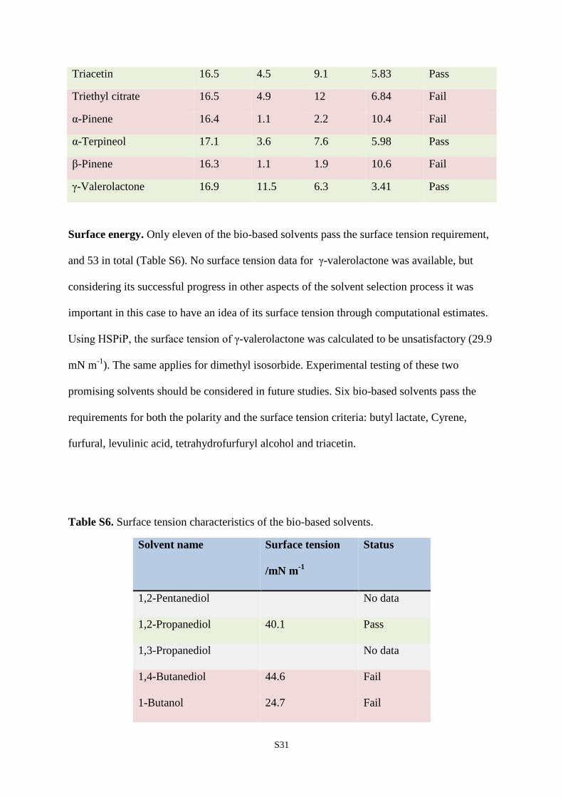
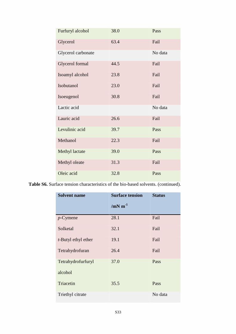
Surface energy. Only eleven of the bio-based solvents pass the surface tension requirement,
and 53 in total (Table S6). No surface tension data for γ-valerolactone was available, but
considering its successful progress in other aspects of the solvent selection process it was
important in this case to have an idea of its surface tension through computational estimates.
Using HSPiP, the surface tension of γ-valerolactone was calculated to be unsatisfactory (29.9
mN m-1). The same applies for dimethyl isosorbide. Experimental testing of these two
promising solvents should be considered in future studies. Six bio-based solvents pass the
requirements for both the polarity and the surface tension criteria: butyl lactate, Cyrene,
furfural, levulinic acid, tetrahydrofurfuryl alcohol and triacetin.
Table S6. Surface tension characteristics of the bio-based solvents.
Solvent name Surface tension
/mN m-1
Status
1,2-Pentanediol No data
1,2-Propanediol 40.1 Pass
1,3-Propanediol No data
1,4-Butanediol 44.6 Fail
1-Butanol 24.7 Fail

S32
2-Butanol 23.4 Fail
2-Methyltetrahydrofuran No data
2-Octanol 26.4 Fail
2-Propanol 20.9 Fail
Acetic acid 27.4 Fail
Acetone 22.7 Fail
Acetyltributyl citrate No data
Butyl lactate 35.0 Pass
Butyric acid 26.7 Fail
Cyrene 33.6 Pass
Diethoxymethane 21.6 Fail
Dimethyl ether 16.0 Fail
Dimethyl isosorbide (Fail)*
Dimethyl sulphoxide 43.0 Pass
d-Limonene 26.9 Fail
Table S6. Surface tension characteristics of the bio-based solvents. (continued).
Solvent name Surface tension
/mN m-1
Status
Ethanol 21.2 Fail
Ethyl acetate 23.8 Fail
Ethyl lactate 29.2 Fail
Ethylene glycol 48.5 Fail
Eugenol 30.9 Fail
Furfural 43.5 Pass
S33
Furfuryl alcohol 38.0 Pass
Glycerol 63.4 Fail
Glycerol carbonate No data
Glycerol formal 44.5 Fail
Isoamyl alcohol 23.8 Fail
Isobutanol 23.0 Fail
Isoeugenol 30.8 Fail
Lactic acid No data
Lauric acid 26.6 Fail
Levulinic acid 39.7 Pass
Methanol 22.3 Fail
Methyl lactate 39.0 Pass
Methyl oleate 31.3 Fail
Oleic acid 32.8 Pass
Table S6. Surface tension characteristics of the bio-based solvents. (continued).
Solvent name Surface tension
/mN m-1
Status
p-Cymene 28.1 Fail
Solketal 32.1 Fail
t-Butyl ethyl ether 19.1 Fail
Tetrahydrofuran 26.4 Fail
Tetrahydrofurfuryl
alcohol
37.0 Pass
Triacetin 35.5 Pass
Triethyl citrate No data
S34
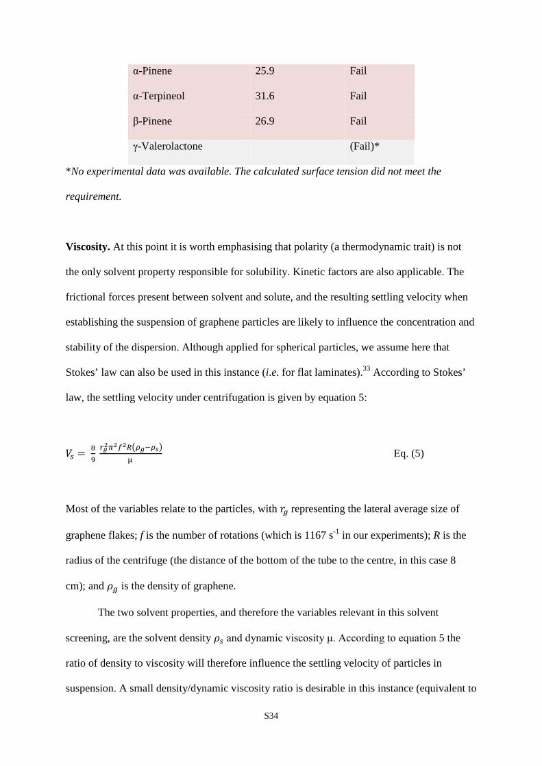
α-Pinene 25.9 Fail
α-Terpineol 31.6 Fail
β-Pinene 26.9 Fail
γ-Valerolactone (Fail)*
*No experimental data was available. The calculated surface tension did not meet the
requirement.
Viscosity. At this point it is worth emphasising that polarity (a thermodynamic trait) is not
the only solvent property responsible for solubility. Kinetic factors are also applicable. The
frictional forces present between solvent and solute, and the resulting settling velocity when
establishing the suspension of graphene particles are likely to influence the concentration and
stability of the dispersion. Although applied for spherical particles, we assume here that
Stokes’ law can also be used in this instance (i.e. for flat laminates).33 According to Stokes’
law, the settling velocity under centrifugation is given by equation 5:
𝑉𝑠 = 89
𝑟𝑔2𝜋2𝑓2𝑅�𝜌𝑔−𝜌𝑠�
µ Eq. (5)
Most of the variables relate to the particles, with 𝑟𝑔 representing the lateral average size of
graphene flakes; f is the number of rotations (which is 1167 s-1 in our experiments); R is the
radius of the centrifuge (the distance of the bottom of the tube to the centre, in this case 8
cm); and 𝜌𝑔 is the density of graphene.
The two solvent properties, and therefore the variables relevant in this solvent
screening, are the solvent density 𝜌𝑠 and dynamic viscosity μ. According to equation 5 the
ratio of density to viscosity will therefore influence the settling velocity of particles in
suspension. A small density/dynamic viscosity ratio is desirable in this instance (equivalent to

S35
the inverse of kinematic viscosity). We have proposed that a low settling velocity caused by
high kinematic viscosity contributes to a higher concentration of dispersed graphene after
centrifugation because of the increased stability of the dispersion. Evidence that viscosity is
also related to the quality of graphene has also been provided (refer to Raman spectroscopy
experiments in the main article and the Experiment Results section of this Supporting
Information).
An arbitrary upper limit to the density/viscosity ratio of 1.20 g mL-1 cP-1 was
implemented so to contain the recognised solvents with known high performance (NMP,
DMF, and 1,2-DCB) but exclude enough solvents to justify the exercise. This produced 127
candidates from 199 entries. This was calculated independently of whether the polarity and
surface tension of each solvent candidate was deemed as suitable or not. Of the solvent
candidates with an ideal density to viscosity ratio, many are plasticisers, diols, and other
glycerol derivatives too polar to qualify as graphene processing solvents (at least using the
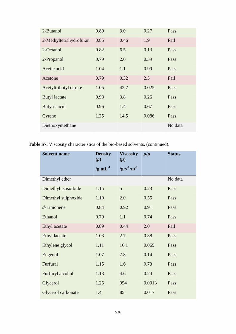
conditions reported here). Most of the bio-based solvents pass this criterion of the
assessment, with the exception of 2-methyltetrahydrofuran, acetone, ethyl acetate, methanol,
and tetrahydrofuran, and 8 further solvents without viscosity data (Table S7).
Table S7. Viscosity characteristics of the bio-based solvents.
Solvent name Density (ρ)
/g mL-1
Viscosity (µ)
/g s-1 m-1
ρ/µ Status
1,2-Pentanediol No data
1,2-Propanediol 1.04 56 0.019 Pass
1,3-Propanediol No data
1,4-Butanediol 1.02 84.9 0.012 Pass
1-Butanol 0.81 2.5 0.32 Pass
S36
2-Butanol 0.80 3.0 0.27 Pass
2-Methyltetrahydrofuran 0.85 0.46 1.9 Fail
2-Octanol 0.82 6.5 0.13 Pass
2-Propanol 0.79 2.0 0.39 Pass
Acetic acid 1.04 1.1 0.99 Pass
Acetone 0.79 0.32 2.5 Fail
Acetyltributyl citrate 1.05 42.7 0.025 Pass
Butyl lactate 0.98 3.8 0.26 Pass
Butyric acid 0.96 1.4 0.67 Pass
Cyrene 1.25 14.5 0.086 Pass
Diethoxymethane No data
Table S7. Viscosity characteristics of the bio-based solvents. (continued).
Solvent name Density (ρ)
/g·mL-1
Viscosity (µ)
/g·s-1·m-1
ρ/µ Status
Dimethyl ether No data
Dimethyl isosorbide 1.15 5 0.23 Pass
Dimethyl sulphoxide 1.10 2.0 0.55 Pass
d-Limonene 0.84 0.92 0.91 Pass
Ethanol 0.79 1.1 0.74 Pass
Ethyl acetate 0.89 0.44 2.0 Fail
Ethyl lactate 1.03 2.7 0.38 Pass
Ethylene glycol 1.11 16.1 0.069 Pass
Eugenol 1.07 7.8 0.14 Pass
Furfural 1.15 1.6 0.73 Pass
Furfuryl alcohol 1.13 4.6 0.24 Pass
Glycerol 1.25 954 0.0013 Pass
Glycerol carbonate 1.4 85 0.017 Pass
S37
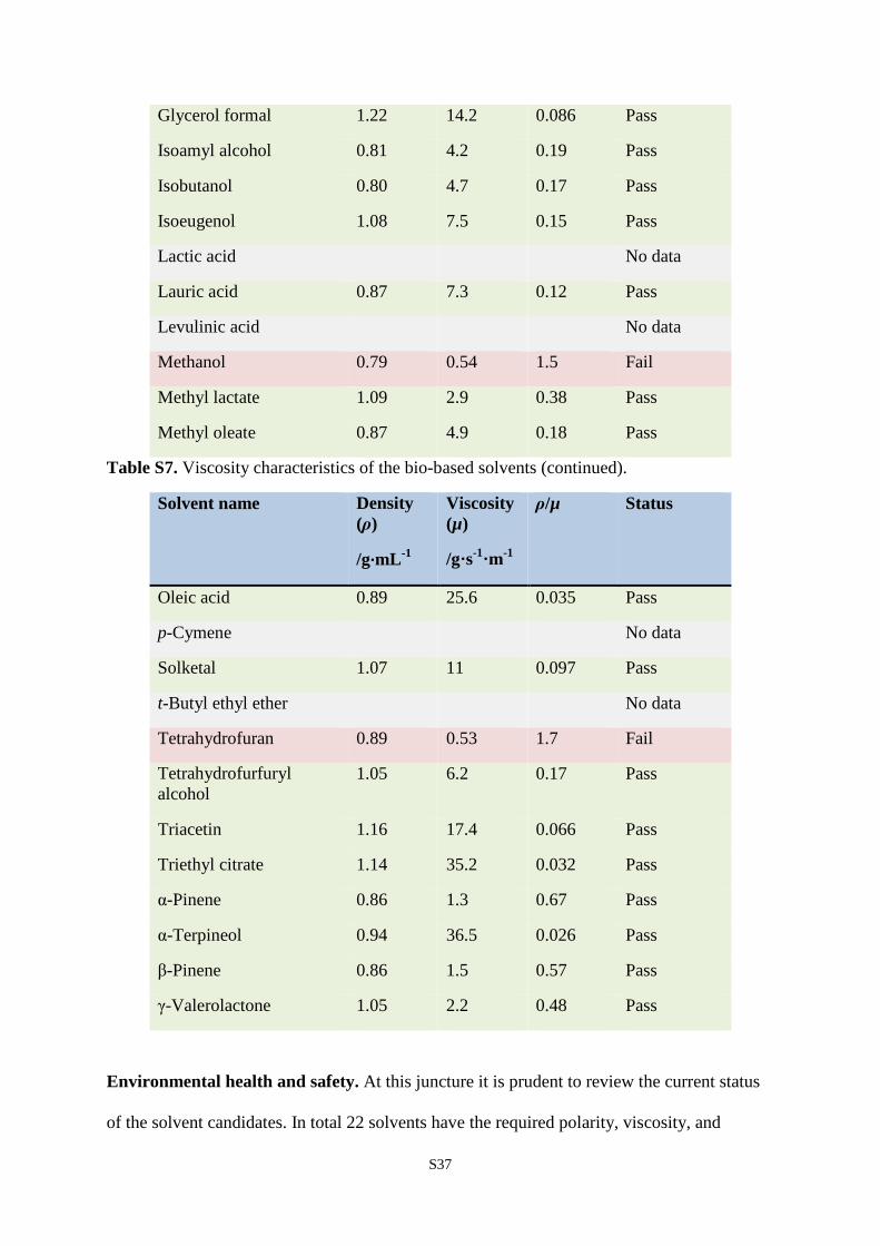
Glycerol formal 1.22 14.2 0.086 Pass
Isoamyl alcohol 0.81 4.2 0.19 Pass
Isobutanol 0.80 4.7 0.17 Pass
Isoeugenol 1.08 7.5 0.15 Pass
Lactic acid No data
Lauric acid 0.87 7.3 0.12 Pass
Levulinic acid No data
Methanol 0.79 0.54 1.5 Fail
Methyl lactate 1.09 2.9 0.38 Pass
Methyl oleate 0.87 4.9 0.18 Pass
Table S7. Viscosity characteristics of the bio-based solvents (continued).
Solvent name Density (ρ)
/g·mL-1
Viscosity (µ)
/g·s-1·m-1
ρ/µ Status
Oleic acid 0.89 25.6 0.035 Pass
p-Cymene No data
Solketal 1.07 11 0.097 Pass
t-Butyl ethyl ether No data
Tetrahydrofuran 0.89 0.53 1.7 Fail
Tetrahydrofurfuryl alcohol
1.05 6.2 0.17 Pass
Triacetin 1.16 17.4 0.066 Pass
Triethyl citrate 1.14 35.2 0.032 Pass
α-Pinene 0.86 1.3 0.67 Pass
α-Terpineol 0.94 36.5 0.026 Pass
β-Pinene 0.86 1.5 0.57 Pass
γ-Valerolactone 1.05 2.2 0.48 Pass
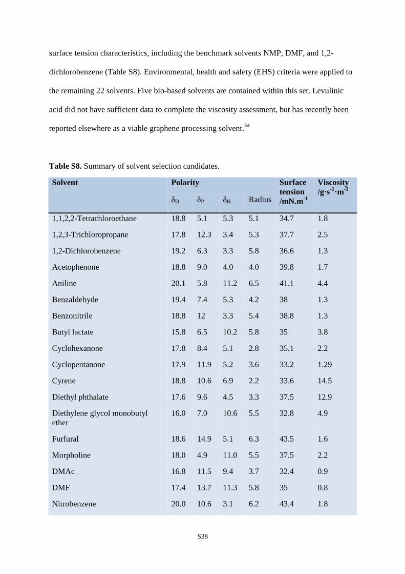
Environmental health and safety. At this juncture it is prudent to review the current status
of the solvent candidates. In total 22 solvents have the required polarity, viscosity, and
S38
surface tension characteristics, including the benchmark solvents NMP, DMF, and 1,2-
dichlorobenzene (Table S8). Environmental, health and safety (EHS) criteria were applied to
the remaining 22 solvents. Five bio-based solvents are contained within this set. Levulinic
acid did not have sufficient data to complete the viscosity assessment, but has recently been
reported elsewhere as a viable graphene processing solvent.34
Table S8. Summary of solvent selection candidates.
Solvent Polarity Surface tension /mN.m-1
Viscosity /g·s-1·m-1
δD δP δH Radius
1,1,2,2-Tetrachloroethane 18.8 5.1 5.3 5.1 34.7 1.8
1,2,3-Trichloropropane 17.8 12.3 3.4 5.3 37.7 2.5
1,2-Dichlorobenzene 19.2 6.3 3.3 5.8 36.6 1.3
Acetophenone 18.8 9.0 4.0 4.0 39.8 1.7
Aniline 20.1 5.8 11.2 6.5 41.1 4.4
Benzaldehyde 19.4 7.4 5.3 4.2 38 1.3
Benzonitrile 18.8 12 3.3 5.4 38.8 1.3
Butyl lactate 15.8 6.5 10.2 5.8 35 3.8
Cyclohexanone 17.8 8.4 5.1 2.8 35.1 2.2
Cyclopentanone 17.9 11.9 5.2 3.6 33.2 1.29
Cyrene 18.8 10.6 6.9 2.2 33.6 14.5
Diethyl phthalate 17.6 9.6 4.5 3.3 37.5 12.9
Diethylene glycol monobutyl ether
16.0 7.0 10.6 5.5 32.8 4.9
Furfural 18.6 14.9 5.1 6.3 43.5 1.6
Morpholine 18.0 4.9 11.0 5.5 37.5 2.2
DMAc 16.8 11.5 9.4 3.7 32.4 0.9
DMF 17.4 13.7 11.3 5.8 35 0.8
Nitrobenzene 20.0 10.6 3.1 6.2 43.4 1.8

S39
NMP 18.0 12.3 7.2 3.0 40.7 1.7
Pyridine 19.0 8.8 5.9 2.7 36.6 0.9
Tetrahydrofurfuryl alcohol 17.8 8.2 12.9 5.3 37 6.2
Triacetin 16.5 4.5 9.1 5.8 35.5 17.4
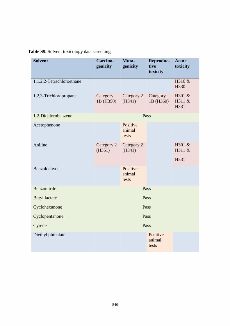
As a first pass greenness assessment, the safety datasheet (obtained from Sigma-
Aldrich) of each of the 22 shortlisted solvents was used to immediately rule out candidates
based on their toxicity profile (Table S9). Any solvent that causes cancer in humans, has been
found to be mutagenic, or is reprotoxic was rejected in line with REACH CMR requirements
(Table S3). Entries in orange in Table S9 indicate likely chronic toxicity in humans based on
animal studies. Solvents that are severely acutely toxic (e.g. represented by any of the hazard
statements H300, H301, H310, H331, H330, H331 as defined in the CLP directive) were also
removed from the final candidate list, leaving only eight solvents remaining. No solvent
candidates of the 22 on the shortlist were classifiable as PBT, although the aquatic toxicity of
several candidates is high (see supplementary spreadsheet file).
S40
Table S9. Solvent toxicology data screening.
Solvent Carcino-genicity
Muta-genicity
Reproduc-tive toxicity
Acute toxicity
1,1,2,2-Tetrachloroethane H310 & H330
1,2,3-Trichloropropane Category 1B (H350)
Category 2 (H341)
Category 1B (H360)
H301 & H311 & H331
1,2-Dichlorobenzene Pass
Acetophenone Positive animal tests
Aniline Category 2 (H351)
Category 2 (H341)
H301 & H311 &
H331
Benzaldehyde Positive animal tests
Benzonitrile Pass
Butyl lactate Pass
Cyclohexanone Pass
Cyclopentanone Pass
Cyrene Pass
Diethyl phthalate Positive animal tests

S41
Table S9. Solvent toxicology data screening. (continued).
Solvent Carcino-genicity
Muta-genicity
Reproduc-tive toxicity
Acute toxicity
Diethylene glycol monobutyl ether
REACH restriction already in place: “Shall not be placed on the market for supply to the general public, as a constituent of spray paints or spray cleaners in aerosol dispensers in concentrations equal to or greater than 3 % by weight” (EU regulation (EC) No 1907/2006).
Furfural Category 2 (H351)
Positive animal tests
H301 & H331
Morpholine Positive animal tests
N,N-Dimethylacetamide Category 2 (H360D)
DMF Category 2 (H360D)
Nitrobenzene Category 1B (H351)
Category 1B (H360F)
H301 & H311 & H331
NMP Category 2 (H360)
Pyridine Pass
Tetrahydrofurfuryl alcohol Category 1B (H360Df)
Triacetin Pass
Greenness assessment. The final phase of the solvent selection process relates to the
greenness of each remaining solvent. The greenness assessment was only applied to the eight
solvent candidates fulfilling the earlier performance requirements and EHS requirements to
reduce the data gathering exercise. Cyrene is the only wholly bio-based solvent remaining.
Butyl lactate is partially bio-based at present, as is triacetin. The technology exists to produce
S42
wholly bio-based butyl lactate and triacetin, but the price and availability of bio-1-butanol
and bio-based acetic acid means for the time being their petrochemical equivalents are used
to produce the downstream solvents. This was not seen as a concern in the long term, with the
lower threshold for bio-based solvents set at 25% bio-based carbon content (Table S4). For
the 5 other solvents (1,2-dichlorobenzene, benzonitrile, cyclohexanone, cyclopentanone, and
pyridine) the lack of a commercially proven renewable feedstock for manufacture is
disadvantageous.
Greenness criteria were selected in an attempted to cover the different aspects of the
solvent life cycle while also being validated by regulations. This exercise is not intended to
rule out any of the final eight solvent candidates, instead its purpose is to create a hierarchy
within these remaining solvents.
Seven physical property and toxicology data sets were obtained and related to
consequential environmental, health and safety effects. The criteria were vapour pressure
(low values are ideal to reduce VOC losses into atmosphere), autoignition temperature and
flash point (for safety considerations), and rat oral LD50 (a health measure). In terms of
environmental issues, lipophilicity (low logP values suggest a low potential for
bioaccumulation) and aquatic toxicity were also considered in addition to biodegradability.
Indicators for these criteria were presented earlier (Table S4). The greenness of the final eight
solvent candidates can be compared to identify the most favourable options. A detailed
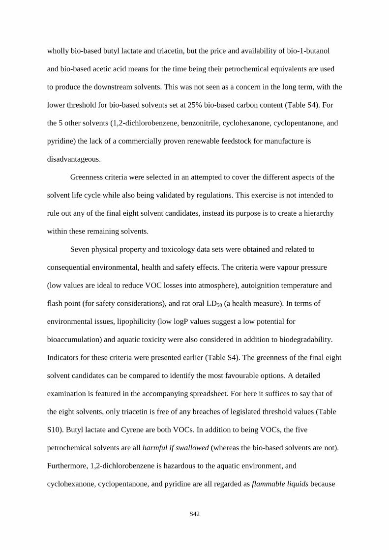
examination is featured in the accompanying spreadsheet. For here it suffices to say that of
the eight solvents, only triacetin is free of any breaches of legislated threshold values (Table
S10). Butyl lactate and Cyrene are both VOCs. In addition to being VOCs, the five
petrochemical solvents are all harmful if swallowed (whereas the bio-based solvents are not).
Furthermore, 1,2-dichlorobenzene is hazardous to the aquatic environment, and
cyclohexanone, cyclopentanone, and pyridine are all regarded as flammable liquids because
S43
of their low flash points. For these reasons butyl lactate, Cyrene, and triacetin were employed
as solvents in experimental graphene processing (Figure S12). The results are reported in the
main article.
Table S10. Solvent greenness issues.
Solvent Breaches of regulatory limits relating to solvent greenness
1,2-Dichlorobenzene CLP 'acute toxicity' threshold (harmful if swallowed); Industrial emissions VOC definition; CLP 'harmful to the aquatic environment'.
Benzonitrile CLP 'acute toxicity' threshold (harmful if swallowed); Industrial emissions VOC definition.
Butyl lactate Industrial emissions VOC definition.
Cyclohexanone CLP 'acute toxicity' threshold (harmful if swallowed); CLP 'flammable liquids' threshold; Industrial emissions VOC definition.
Cyclopentanone CLP 'acute toxicity' threshold (harmful if swallowed); CLP 'flammable liquids' threshold; Industrial emissions VOC definition.
Cyrene Industrial emissions VOC definition.
Pyridine CLP 'acute toxicity' threshold (harmful if swallowed); CLP 'flammable liquids' threshold; Industrial emissions VOC definition.
Triacetin None.
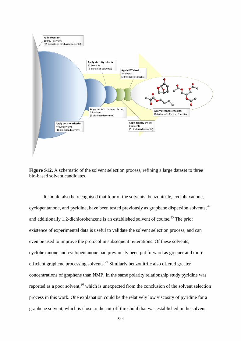
S44
Figure S12. A schematic of the solvent selection process, refining a large dataset to three bio-based solvent candidates.
It should also be recognised that four of the solvents: benzonitrile, cyclohexanone,
cyclopentanone, and pyridine, have been tested previously as graphene dispersion solvents,26
and additionally 1,2-dichlorobenzene is an established solvent of course.35 The prior
existence of experimental data is useful to validate the solvent selection process, and can
even be used to improve the protocol in subsequent reiterations. Of these solvents,
cyclohexanone and cyclopentanone had previously been put forward as greener and more
efficient graphene processing solvents.29 Similarly benzonitrile also offered greater
concentrations of graphene than NMP. In the same polarity relationship study pyridine was
reported as a poor solvent,26 which is unexpected from the conclusion of the solvent selection
process in this work. One explanation could be the relatively low viscosity of pyridine for a
graphene solvent, which is close to the cut-off threshold that was established in the solvent

S45
selection process. Also note however that other reports show the successful use of pyridine as
a graphene processing solvent,36 and so the distinction between good and poor graphene
processing solvents remains slightly elusive. That is why a multi-criteria solvent selection
protocol was designed, and a number of solvent candidates shortlisted rather than only one.
Overview of advantages of Cyrene compared to NMP. Table S11 provides the numerical data given in Figure 1 of the main article.
Table S11. Relevant properties of Cyrene and NMP.
Solvent properties NMP Cyrene
Phys
ical
pro
pert
ies
Density (ρ), g cm-3 1.03 1.24
Viscosity (µ), cP 1.7 10.5
Surface tension (γ), mN m-1 40.7 33.6
Surface energy (ε),* mN m-1 70.5 63.4
Dispersive Hansen parameter (δD),§ MPa0.5 18.0 18.8
Polar Hansen parameter (δP),§ MPa0.5 12.3 10.6
Hydrogen bonding Hansen parameter (δH),§ MPa0.5 7.2 6.9
Envi
ronm
enta
l he
alth
and
safe
ty
cons
ider
atio
ns Vapor pressure, mmHg 0.34 0.21
Flash point (closed cup), °C 92 108
Bio-based content 0% 100%
logP -0.38 -1.52 ∗Calculated according to the equation: 𝛾 = 𝜀 − 𝑇𝑇, where the surface entropy, S takes the
same value for both solvents,3 of S ∼ 0.1 mJ m-2 K-1
§Calculated with HSPiP software.
S46
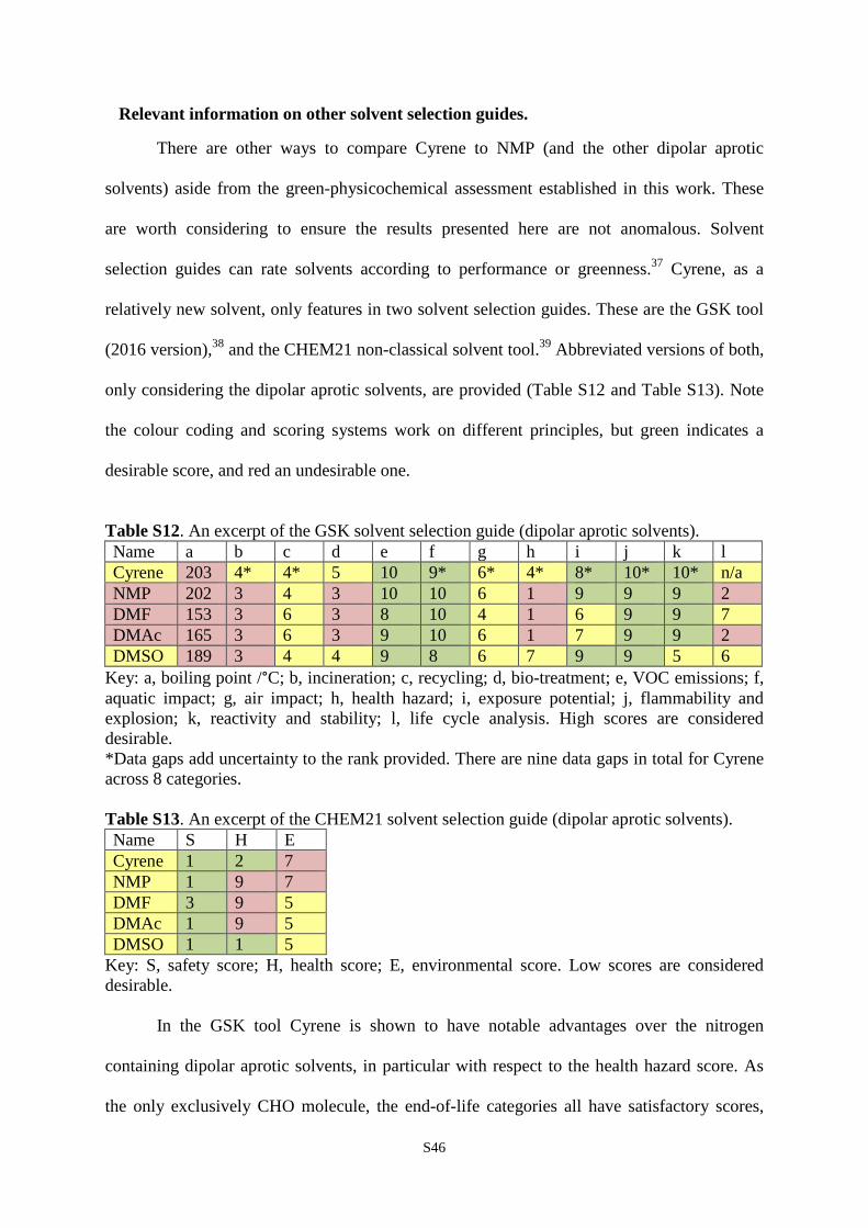
Relevant information on other solvent selection guides.
There are other ways to compare Cyrene to NMP (and the other dipolar aprotic
solvents) aside from the green-physicochemical assessment established in this work. These
are worth considering to ensure the results presented here are not anomalous. Solvent
selection guides can rate solvents according to performance or greenness.37 Cyrene, as a
relatively new solvent, only features in two solvent selection guides. These are the GSK tool
(2016 version),38 and the CHEM21 non-classical solvent tool.39 Abbreviated versions of both,
only considering the dipolar aprotic solvents, are provided (Table S12 and Table S13). Note
the colour coding and scoring systems work on different principles, but green indicates a
desirable score, and red an undesirable one.
Table S12. An excerpt of the GSK solvent selection guide (dipolar aprotic solvents). Name a b c d e f g h i j k l Cyrene 203 4* 4* 5 10 9* 6* 4* 8* 10* 10* n/a NMP 202 3 4 3 10 10 6 1 9 9 9 2 DMF 153 3 6 3 8 10 4 1 6 9 9 7 DMAc 165 3 6 3 9 10 6 1 7 9 9 2 DMSO 189 3 4 4 9 8 6 7 9 9 5 6
Key: a, boiling point /°C; b, incineration; c, recycling; d, bio-treatment; e, VOC emissions; f, aquatic impact; g, air impact; h, health hazard; i, exposure potential; j, flammability and explosion; k, reactivity and stability; l, life cycle analysis. High scores are considered desirable. *Data gaps add uncertainty to the rank provided. There are nine data gaps in total for Cyrene across 8 categories. Table S13. An excerpt of the CHEM21 solvent selection guide (dipolar aprotic solvents). Name S H E Cyrene 1 2 7 NMP 1 9 7 DMF 3 9 5 DMAc 1 9 5 DMSO 1 1 5
Key: S, safety score; H, health score; E, environmental score. Low scores are considered desirable.
In the GSK tool Cyrene is shown to have notable advantages over the nitrogen
containing dipolar aprotic solvents, in particular with respect to the health hazard score. As
the only exclusively CHO molecule, the end-of-life categories all have satisfactory scores,
S47
helped because no nitrogen or sulphur containing by-products form during incineration or
biological waste treatments. As a word of caution, the complete properties of Cyrene needed
to fulfil the GSK assessment are yet to all be determined. This may cause some of the scores
to increase or decrease in the future as more data becomes available. Similarly, note that a
score based on life cycle assessment is not possible for Cyrene yet.
The CHEM21 guide for use in the pharmaceutical industry appears less
comprehensive by comparison, only having three categories. However there is a benefit to
summarising the relevant data so succinctly for easier interpretation. What this does mean is
that many considerations are behind each score and so the reason for the outcome is not
immediately clear. The undesirable environment (E) score of Cyrene is actually due to its
high boiling point, included in the assessment to recognise that energy intensive distillation is
required in pharmaceutical product synthesis to separate and recycle solvents. Otherwise
Cyrene is recognised as a green solvent.
It is important to remember that it is not only greenness that dictates solvent
substitution, technical performance is also vital but it is very much specific to each different
application. A solvent selection guide cannot tell you whether a solvent will be suitable for a
process or formulation, or why that is so. This is why we did not rely on solvent selection
guides to identify solvents for graphene production by liquid exfoliation. Furthermore,
solvent selection guides are usually restricted to the set of solvents provided, although in this
respect the CHEM21 assessment is easily transferable to new solvents. In this work we were
able to screen a much larger number of solvents that would be feasible to display in terms of
a solvent selection guide.
S48
References
1. Court, G. R.; Lawrence, C. H.; Raverty, W. D; Duncan, A. J. Method for converting
lignocellulosic materials into useful chemicals. World patent 2011, WO 2011000030
A1.
2. Sherwood, J.; De bruyn, M.; Constantinou, A.; Moity, L.; McElroy,C. R.; Farmer, T.
J.; Duncan, T.; Raverty, W.; Hunt, A. J.; Clark, J. H. Dihydrolevoglucosenone
(Cyrene) as a bio-based alternative for dipolar aprotic solvents. Chem. Commun.
2014, 50, 9650-9652.
3. Hernandez,Y.; Nicolosi, V.; Lotya, M.; Blighe, F. M.; Sun, Z.; De, S.; McGovern, I.
T.; Holland, B.; Byrne, M.; Gun'Ko, Y. K.; Boland, J. J.; Niraj, P.; Duesberg, G.;
Krishnamurthy, S.; Goodhue, R.; Hutchison, J.; Scardaci, V.; Ferrari, A. C.; Coleman,
J. N. High-yield production of graphene by liquid-phase exfoliation of graphite. Nat.
Nano. 2008, 3, 563-568.
4. Graphenea. Graphenea Monolayer Graphene film - Product Datasheet. Available
from:
http://cdn.shopify.com/s/files/1/0191/2296/files/Graphenea_Monolayer_Film_Datash
eet_2014-03-25.pdf?2923 (accessed 21/10/2015).
5. Wang, S.; Zhang, Y.; Abidi, N.; Cabrales, L. Wettability and surface free energy of
graphene films. Langmuir 2009, 25, 11078-11081.
6. Coleman, J. N. Liquid exfoliation of defect-free graphene. Acc. Chem. Res. 2013, 46,
14-22.
7. Rafiee, J.; Mi, X.; Gullapalli, H.; Thomas, A. V.; Yavari, F.; Shi, Y.; Ajayan, P. M.;
Koratkar, N. A. Wetting transparency of graphene. Nat. Mater. 2012, 11, 217-222.
S49
8. Taherian, F.; Marcon, V.; van der Vegt, N. F. A.; Leroy, F. What is the contact angle
of water on graphene? Langmuir 2013, 29, 1457-1465.
9. Salavagione, H. J.; Martínez, G.; Ellis, G. Graphene-Based Polymer Nanocomposites.
In Physics And Applications Of Graphene - Experiments. Mikhailov, S., Eds.; InTech:
Vienna, 2011; pp 169-192.
10. Li, Z.; Wang, Y.; Kozbial, A.; Shenoy, G.; Zhou, F.; McGinley, R.; Ireland, P.;
Morganstein, B.; Kunkel, A.; Surwad, S. P.; Li, L.; Liu, H. Effect of airborne
contaminants on the wettability of supported graphene and graphite. Nat. Mater. 2013,
12, 925-931.
11. Li, X.; Cai, W.; An, J.; Kim, S.; Nah, J.; Yang, D.; Piner, R.; Velamakanni, A.; Jung,
I.; Tutuc, E.; Banerjee, S. K.; Colombo, L.; Ruoff, R. S. Large-area synthesis of high-
quality and uniform graphene films on copper foils. Science 2009, 324, 1312-1314.
12. Reina, A.; Jia, X.; Ho, J.; Nezich, D.; Son, H.; Bulovic, V.; Dresselhaus, M. S.; Kong,
J. Large area, few-layer graphene films on arbitrary substrates by chemical vapor
deposition. Nano. Lett. 2009, 9, 30-35.
13. Malard, L. M.; Pimenta, M. A.; Dresselhaus, G.; Dresselhaus, M. S. Raman
spectroscopy in graphene. Phys. Rep. 2009, 473, 51-87.
14. Pimenta, M. A.; Dresselhaus, G.; Dresselhaus, M. S.; Cançado, L. G.; Jorio, A.; Saito,
R. Studying disorder in graphite-based systems by Raman spectroscopy. Phys. Chem.
Chem. Phys. 2007, 9, 1276-1290.
15. Ferrari, A. C. Raman spectroscopy of graphene and graphite: disorder, electron–
phonon coupling, doping and nonadiabatic effects. Solid State Commun. 2007, 143,
47-57.
S50
16. Hao, Y.; Wang, Y.; Wang, L.; Ni, Z.; Wang, Z.; Wang, R.; Koo, C. K.; Shen, Z.;
Thong, J. T. L. Probing layer number and stacking order of few-layer graphene by
Raman spectroscopy. Small 2010, 6, 195-200.
17. Cançado, L. G.; Takai, K.; Enoki, T.; Endo, M.; Kim, Y. A.; Mizusaki, H.; Jorio, A.;
Coelho, L. N.; Magalhães-Paniago, R.; Pimenta, M. A. General equation for the
determination of the crystallite size La of nanographite by Raman spectroscopy. Appl.
Phys. Lett. 2006, 88, 163106.
18. Cançado, L. G.; Jorio, A.; Martins Ferreira, E. H.; Stavale, F.; Achete, C. A.; Capaz,
R. B.; Moutinho, M. V. O.; Lombardo, A.; Kulmala, T. S.; Ferrari, A. C. Quantifying
defects in graphene via Raman spectroscopy at different excitation energies. Nano
Lett. 2011, 11, 3190-3196.
19. Khan, U.; O’Neill, A.; Lotya, M.; De, S.; Coleman, J. N. High-concentration solvent
exfoliation of graphene. Small 2010, 6, 864-871.
20. Sun, Z.; Vivekananthan, J.; Guschin, D. A.; Huang, X.; Kuznetsov, V.; Ebbinghaus,
P.; Sarfraz, A.; Muhler, M.; Schuhmann, W. High concentration graphene dispersions
with minimal stabilizer: a scaffold for enzyme immobilization for glucose oxidation.
Chem. Eur. J. 2014, 20, 5752-5761.
21. Gani, R.; Jiménez-González, C.; Constable, D. J. C. Method for selection of solvents
for promotion of organic reactions. Computers & Chemical Engineering 2005, 29,
1661-1676.
22. O’Neill, A.; Khan, U.; Nirmalraj, P. N.; Boland, J.; Coleman, J. N. Graphene
dispersion and exfoliation in low boiling point solvents. J. Phys. Chem. C 2011, 115,
5422-5428.
S51
23. Cheng, Q.; Debnath, S.; Gregan, E.; Byrne, H. J. Ultrasound-assisted SWNTs
dispersion: effects of sonication parameters and solvent properties. J. Phys. Chem. C
2010, 114, 8821-8827.
24. Yousefinejad, S.; Honarasa, F.; Abbasitabar, F.; Arianezhad, Z. New LSER model
based on solvent empirical parameters for the prediction and description of the
solubility of buckminsterfullerene in various solvents. J. Solution Chem. 2013, 42,
1620-1632.
25. Kim, J. H.; Lee, J. H. Preparation of graphite nanosheets by combining microwave
irradiation and liquid-phase exfoliation. J. Ceram. Process. Res. 2014, 15, 341-346.
26. Hernandez, Y.; Lotya, M.; Rickard, D.; Bergin, S. D.; Coleman, J. N. Measurement of
multicomponent solubility parameters for graphene facilitates solvent discovery.
Langmuir 2010, 26, 3208-3213.
27. Yi, M.; Shen, Z. G.; Zhang, X. J.; Ma, S. L. Achieving concentrated graphene
dispersions in water/acetone mixtures by the strategy of tailoring hansen solubility
parameters. J. Phys. D: Appl. Phys. 2013, 46, 025301.
28. CEN/TS 16766:2015. Bio-based solvents - Requirements and test methods. CEN/TC
411 Bio-based products: European Committe for Standardization (2015).
29. Hansen, C. M. In Hansen Solubility Parameters: A User's Handbook; CRC press:
Boca Raton, 2007.
30. Bergin, S. D.; Sun, Z.; Rickard, D.; Streich, P. V.; Hamilton, J. P.; Coleman, J. N.
Multicomponent solubility parameters for single-walled carbon nanotube−solvent
mixtures. ACS Nano 2009, 3, 2340-2350.
31. Shin, Y. J.; Wang, Y.; Huang, H.; Kalon, G.; Wee, A. T. S.; Shen, Z.; Bhatia, C. S.;
Yang, H. Surface-energy engineering of graphene. Langmuir 2010, 26, 3798-3802.

S52
32. Lim, H. J.; Lee, K.; Cho, Y. S.; Kim, Y. S.; Kim, T.; Park, C. R. Experimental
consideration of the hansen solubility parameters of as-produced multi-walled carbon
nanotubes by inverse gas chromatography. Phys. Chem. Chem. Phys. 2014, 16,
17466-17472.
33. Xiong, B.; Cheng, J.; Qiao, Y.; Zhou, R.; He, Y.; Yeung, E. S. Separation of nanorods
by density gradient centrifugation. J. Chromatogr. A 2011, 1218, 3823-3829.
34. Sharma, M.; Mondal, D.; Singh, N.; Prasad, K. Biomass derived solvents for the
scalable production of single layered graphene from graphite. Chem. Comm. 2016.
DOI: 10.1039/C6CC00256K.
35. Hamilton, C. E.; Lomeda, J. R.; Sun, Z.; Tour, J. M.; Barron, A. R. High-yield organic
dispersions of unfunctionalized graphene. Nano Lett. 2009, 9, 3460-3462.
36. Park, K. H.; Kim, B. H.; Song, S. H.; Kwon, J.; Kong, B. S.; Kang, K.; Jeon, S.
Exfoliation of non-oxidized graphene flakes for scalable conductive film. Nano Lett.
2012, 12, 2871-2876.
37. F. P. Byrne, S. Jin, G. Paggiola, T. H. M. Petchey, J. H. Clark, T. J. Farmer, A. J.
Hunt, C. R. McElroy and J. Sherwood, Tools and techniques for solvent selection:
green solvent selection guides. Sustainable Chemical Processes, 2016, 4, 7.
38. C. M. Alder, J. D. Hayler, R. K. Henderson, A. M. Redman, L. Shukla, L. E. Shuster
and H. F. Sneddon, Updating and further expanding GSK's solvent sustainability
guide. Green Chem., 2016, 18, 3879-3890.
39. D. Prat, A. Wells, J. Hayler, H. Sneddon, C. R. McElroy, S. Abou-Shehada and P. J.
Dunn, CHEM21 selection guide of classical- and less classical-solvents. Green
Chem., 2016, 18, 288-296.