Embed Size (px)
Citation preview

Identification of Foliar Diseases in Cotton Crop Alexandre A. Bernardes, Jonathan G. Rogeri, Roberta B. Oliveira, Norian Marranghello and Aledir S. Pereira Universidade Estadual Paulista (UNESP) / Instituto de Biociências, Letras e Ciências Exata (IBILCE), São José do Rio Preto, São Paulo, Brasil. Alex F. Araujo and João Manuel R.S. Tavares Instituto de Engenharia Mecânica e Gestão Industrial, Faculdade de Engenharia, Universidade do Porto, Portugal.
([email protected], [email protected], [email protected], [email protected], [email protected], [email protected], [email protected])
Abstract
The manifestation of pathogens in plantations is the most important cause of losses in several crops. These usually represent less income to the farmers due to the lower product quality as well as higher prices to the consumer due to the smaller offering of goods. The sooner the disease is identified the sooner one can control it through the use of agrochemicals, avoiding great damages to the plantation. This chapter introduces a method for the automatic classification of cotton diseases based on the feature extraction of foliar symptoms from digital images. The method uses the energy of the wavelet transform for feature extraction and a Support Vector Machine for the actual classification. Five possible diagnostics are provided: 1) healthy (SA), 2) injured with Ramularia disease (RA), 3) infected with Bacterial Blight (MA), 4) infected with Ascochyta Blight (AS), or 5) possibly infected with an unknown disease.

1. Introduction
The art of growing food is fundamental for the human subsistence. The manifestation of diseases causes many damages, either financial or in terms of the quality of the crops, causing considerable losses if the degree of infestation is high. Several agrochemicals are applied to the plantation in an effort to minimize and control pathogens. However, the agrochemicals are usually harmful to the human health, can increase production costs, and may contaminate water and soil [1].
Aiming at minimizing agrochemicals use, ensuring product quality and minimizing inherent agricultural production problems, computer applications have been developed and revealed high efficacy. The use of computers in agriculture has been subject of several scientific works, many of them focusing on the identification of diseases through foliar symptoms in various cultivars, such as: wheat [1], cotton [2], rice [3, 4, 5], apple [6], orchid [7], cucumber [8, 9], rose [10], rubber tree [11], soybean [12, 13], and grape [14].
In this work, we propose the identification of foliar diseases in cotton crop because, being a pillar of textile production, is a cultivar of great economic importance. The Brazilian textile industry consumes around a million tons of cotton fiber a year, which means that cotton is particularly important for the economy, creating thousands of job positions both in the agricultural and industrial sectors of the economy.
The main goal of the computational system developed is to identify from images the existence, or not, of pathogens in a given plantation. If no pathogens are found the plantation is classified as healthy (SA). Otherwise the image under consideration undergoes a second stage of analysis in view of the automatic classification of the disease. The pathogens that are considered in this stage are among the most frequently observed in Brazil; additionally, they usually disseminate rapidly throughout the infected plantation, and can be identified with the use of specific chemical products. Three diseases within this category can be identified by the developed system: Ramularia (RA), Bacterial Blight (BA), and Ascochyta Blight (AS). If a pathogen is found that cannot be classified as one of these three diseases, the correspondent image is classified as being infected by an unknown disease.

In recent works [15, 16] it was concluded that the decomposition of the image to be classified in color elements, can lead to successfully classification of natural objects. Thus, we used several alternatives of color patterns, such as RGB, HSV, I3a and I3b, as well as the gray levels of the image under analysis in an attempt to improve the distinction of the pathogen classes. The color channels I3a and I3b are obtained by changing the original color standard I1I2I3 [15]. One of the most widely used solutions to obtain compact feature representations of an input image is by using the energy of its wavelet transform. The result of such wavelet transform is a set of feature vectors that are usually used during the further classification phases. In the proposed method, we use a support vector machine (SVM) properly trained to identify the aforementioned diseases.
1.1 Channels I3a and I3b
Channels RGB and HSV are well known in current literature. However, channels I3a and I3b are not so. They are obtained by following the modifications proposed by Camargo [15] on the color channel I3 of the model I1I2I3 defined by Ohta [16]. Such modifications are produced in constants m and d of the equation:
𝐼3 = ((𝑚 × 𝐼𝐺(𝑖,𝑗))∑ 𝐼𝑅(𝑖,𝑗) ∑ 𝐼𝐵(𝑖,𝑗))/𝑑, (1)
where I is an image defined in the color space RGB, i and j represent the coordinates of the Cartesian axes, and IR, IG, and IB are the values corresponding to the color channels, which can vary between 0 (zero) and 255. The changes in the values of the constants m and d are the channels I3a and I3b, as defined by Eq. (2) for channel I3a and by Eq. (3) for channel I3b, respectively. In order to distinguish injured leave areas in several crops, including cotton, m=2.5 has been used for channel I3a, and d=2 has been used for channel I3b. These values have been defined by Camargo [15] through experimentation.
𝐼3𝑎 = ((2.5 × 𝐼𝐺(𝑖,𝑗))∑ 𝐼𝑅(𝑖,𝑗) ∑ 𝐼𝐵(𝑖,𝑗))/4, (2)

𝐼3𝑏 = ((2 × 𝐼𝐺(𝑖,𝑗))∑ 𝐼𝑅(𝑖,𝑗) ∑ 𝐼𝐵(𝑖,𝑗))/2. (3)
1.2 Discrete Wavelet Transform
By applying a Discrete Wavelet Transform (DWT) to an input image, such image can be decomposed into four regions, usually known as sub-bands. Fig. 1 displays the scheme according to which the regions are organized in the original image after being processed by a DWT. Region A tends to cluster the (low-frequency) approximation coefficient of lines and columns of the image; region DL corresponds to the clustering of the line details and column approximations; similarly, region DC corresponds to the clustering of the line approximations and column details; and region D clusters (high-frequency) detail coefficients of lines and columns.
A DL
DC D
Fig. 1. Wavelet decomposition scheme.
Similarly, a 2D image is a bi-dimensional signal to which successive decompositions can be applied. DWT decomposition of an image in three levels is schematically represented in Fig. 2. At the first decomposition level, the sub-bands A1 (approximation coefficient of lines and columns of the first level – A), “8” (line detail coefficients – DL), “9” (line and column detail coefficients – D), and “10” (column detail coefficients – DC) are presented. The second level of decomposition is applied to the approximation coefficient A1, which is in turn decomposed into for sub-bands: A2(A), “5” (DL), “6” (D) e “7” (DC). For the third level of decomposition, region A2 is divided into four other sub-bands: “1” (A), “2” (DL), “3” (D) e “4” (DC). It can be observed that from Fig. 2 the first level decomposition is always done with respect to the
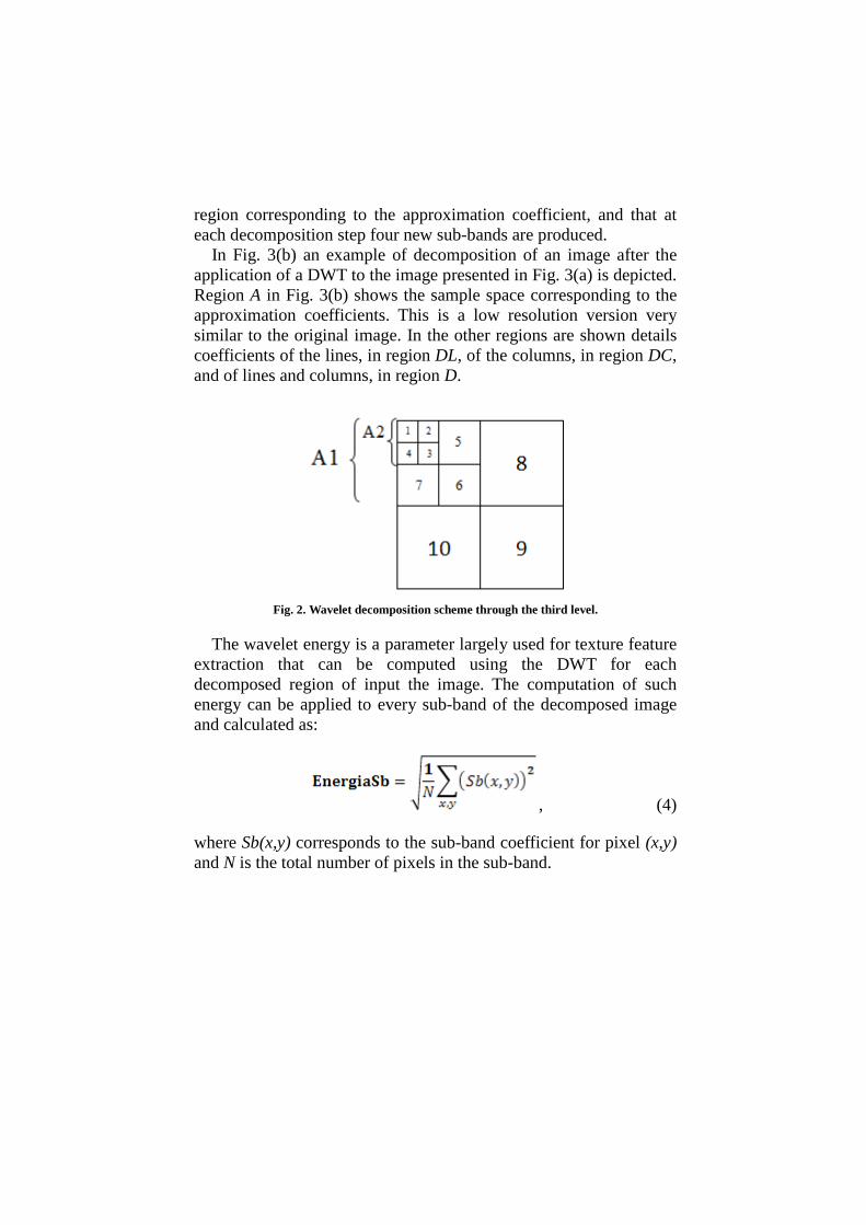
region corresponding to the approximation coefficient, and that at each decomposition step four new sub-bands are produced.
In Fig. 3(b) an example of decomposition of an image after the application of a DWT to the image presented in Fig. 3(a) is depicted. Region A in Fig. 3(b) shows the sample space corresponding to the approximation coefficients. This is a low resolution version very similar to the original image. In the other regions are shown details coefficients of the lines, in region DL, of the columns, in region DC, and of lines and columns, in region D.
Fig. 2. Wavelet decomposition scheme through the third level.
The wavelet energy is a parameter largely used for texture feature extraction that can be computed using the DWT for each decomposed region of input the image. The computation of such energy can be applied to every sub-band of the decomposed image and calculated as:
, (4)
where Sb(x,y) corresponds to the sub-band coefficient for pixel (x,y) and N is the total number of pixels in the sub-band.

(a)
(b)
Fig.3. Example of the decomposition of an original image (a) when applying DWT to the first level (b).
1.3 Support Vector Machine
For feature classification, the method presented in this work uses an Artificial Intelligence technique largely employed in binary classification, known as Support Vector Machine (SVM). This technique can achieve very interesting performances in several practical applications and, in many cases, performances superior to other learning algorithms such as Artificial Neural Networks [17]. SVMs are mainly used in pattern recognition, image processing, machine learning and bioinformatics [18]. In 1992 Vladimir Vapnik and co-workers [19] developed a strategy to separate nonlinear hyperplanes using kernel functions to modify the entry space of a higher dimensional space in which the data are linearly separable. The most usual kernels to be found in such cases are: linear, Gaussian and polynomial. In this work, the Gaussian kernel was used [17].
SVM machine learning technique is based on the structural risk minimization principle. It aims at minimizing the training set related error so as to control the empirical risk. Thus, avoiding noise to appear in place of the general features expected to provide for generalization, i. e., recognition of classes not included in the initial training of the classifier.
The dividing hyperplane is a surface that splits the feature space into two sub-spaces. An element is classified as belonging to class -1 if it is closer to the negative margin, and is classified to class +1 if it
A
DC
DL
D

is closer to the positive margin. Be {(𝑥1���⃗ ,𝑦1); (𝑥2����⃗ , 𝑦2);⋯ (𝑥𝑛����⃗ ,𝑦𝑛)} a training vector set belonging to the two linearly separable classes W1, defined by the output yi=+1, and W2, defined by the output yi=-1. The goal of the SVM is to search for the hyperplane with the largest possible separation margin between the vectors of the two classes. This principle is illustrated in Fig. 4, being class W1 represented by the set of triangles and class W2 by the set of circles. These two classes are linearly separable by the maximum separation margin δ, defined as the summation of the distances from the hyperplane to the closest class separation point corresponding to the optimum separation. It is worth noting that the vectors defining the limits of the hyperplane are known as support vectors.
Fig. 4. Linear separation of classes W1 and W2 in terms of a hyperplane.
There are various possibilities to categorize an element into one of several classes. For instance, if one needs to classify an element into one of two classes, a classification system should be created to embed one net for each class, being each net trained independently. Figure 5 exemplifies this classification process: R1 is trained as belonging to class 1, and net R2 is trained as belonging to class 2. During the classification process, an element is submitted to both nets producing values n1 from R1 and n2 from R2. If n1 is closer to 1 (one) than n2, then the element is considered as belonging to class 1, otherwise it is sorted to class 2. Thus, the element under consideration is always classified as belonging to the class associated to the n value which is closer to 1 (one).
separation margin
W2
W1
optimum hyperplane
δ

Fig. 5. Example of the SVM classification system using two classes: R1 corresponds to net 1 trained as class 1 and R2 corresponds to net 2 trained as class 2; n1 and n2 are the values
obtained from the classification of the elements of the corresponding nets.
2. Materials and Methods
2.1 Materials
420 images of the foliar region of cotton have been obtained from two different sources and combined into one dataset. One set of images was provided by Dr. Nelson Suassuna, phytopathologist, researcher at Embrapa Cotton, in Campina Grande, Brazil [20], and the other set was obtained from the site “Forestry Images” [21] and used to complement Dr. Suassuna’s image set.
The images under study are quite different in terms of dimension, bright, contrast and resolution. Such heterogeneity makes hardly the successfully classification of the dataset elements. As an example, in Fig. 6 some images of healthy regions of cotton leaves are displayed in which the differences among image features can be observed. Besides these discrepancies, the infected leaves present several degrees of severity, as can be observed in the images included in Fig. 7. In Fig. 7(a) it is shown the foliar region in an initial stage of MA pathogen infection, which is characterized by wet-like spots with a dark-green color. In Fig.7(b), the infected leaf is presented in an intermediate stage of the disease that is characterized by small brown spots with tinny yellowish regions. In Fig. 7(c), the disease can be observed in an advanced stage in which the injured region is brown and yellow and is spread almost all over the leaf.
R2 R1
Element
n1
n2

Fig. 6. Some images of healthy foliar regions of cotton leaves.
(a)
(b)
(c)
Fig. 7. Degrees of severity of MA disease in cotton crop: initial stage (a), intermediate stage (b) and advanced stage (c).
2.2. Proposed Method
In this section, we describe how the proposed system was implemented to sort the images under analysis into one of five classes. The Bloodshed Dev-C++ integrated development environment, version 4.9.9.2, was used for the implementation of the system in C and C++, while for image processing and analysis the OpenCV, version 1.0 cr, was used.
The classification process was divided into two phases: Phase 1: Find the best feature vector for each class; and Phase 2: Produce the final classification from the best results
obtained in phase 1.

2.2.1. Phase 1: Find the best feature vectors
The goal of this phase is to find the best feature vector representing each class. In order to achieve it, the following steps were adopted:
a) The input image is decomposed in various color channels (R, G, B, H, S, V, I3a, I3b, and grey levels);
b) Apply the DWT to the third level to each color channel; c) Compute the wavelet energy for each sub-band and compose
the feature vectors; d) Develop the SVM classification environment; e) Undergo the SVM training and testing; f) Select the best feature vectors.
a) Image Decomposition
Image decomposition is the first step of the proposed method. Each image of the data bank is read in the RGB color model, and decomposed into the R, G, and B channels. From this decomposition, the input image is transformed to the HSV color space, to channels I3a and I3b, and to grey levels.
b) DWT down to the third level
Decomposition using the DWT to the third level is applied to each of the nine color channels. When an image is decomposed into three levels ten sub-bands are obtained (Fig. 2). It should be noted that each sub-band is identified by a number between 1 (one) and 10. Region A1 and the sub-bands identified by 8, 9, and 10, are produced by the first level of DWT decomposition. Region A2 and the sub-bands 5, 6, and 7, correspond to the second level of DWT decomposition. Finally, the third level is composed by sub-bands 1, 2, 3, and 4, respectively.
c) Energy of each sub-band
The wavelet energy for each sub-band is computed after applying DWT to the third level. The resulting values are inserted into the

corresponding feature vector. It can be noted from Fig. 8 that such vectors are composed by ten elements, in each of which the related sub-band energy value is stored. Each vector element is identified by an integer number.
Feature Vector 1 2 3 4 5 6 7 8 9 10
Fig. 8. Example of a feature vector used in our system.
d) SVM Classification Environment
The used net architecture of the system developed is displayed in Fig. 9. From this figure, it can be noted that 10 input elements are used. The corresponding feature vector value is assigned to each input. The intermediate, or hidden, layer presents a number of neurons equal to the number N of training examples. This choice for the number of neurons of the hidden layer improves the net convergence characteristics [17]. The chosen net mapping function, known as kernel, has been the Gaussian one.
Fig. 9. SVM architecture used in our system.
In order to assess the proposed system, a sub-set of the images
(feature vectors) was used in the system training. The remaining set was afterwards used for testing. It is worth noting that during the training phase, there is a corresponding output for each input, known as supervised training approach. The output 1 indicates that the element belongs to a class, and output -1 indicates that the element is not a member of the associated class.
Features Vector of
input
K(x,x1)
K(x,x2)
K(x,xN)
⁞ ⁞
1
2
10
⁞ wS
w2
w1
y
Input unit of size 10 Hidden layer size equal to the
number of examples of Training
Linear outputs
Output

e) SVM Training and Testing
The classification process of the system developed has been divided into two stages:
Stage 1: The leaf image is labeled as healthy (SA) or injured (LE);
Stage 2: Only for injured images that have been associated to one of the three possible pathogens (RA, MA, or AS).
As such, it has been possible to choose the best descriptor, i. e., the feature vector to represent each class.
To find the best descriptor for each class in each stage, twelve different wavelet coefficients were computed for each color channel, resulting in twelve feature vectors. In Table 1 each wavelet coefficient used is indicated and associated to the corresponding support numbers as well as to the abbreviations used, namely: Bey18, Coi12, Coi30, Dau4, Dau14, Dau34, Dau64, Dau76, Haar, Sym8 and Vai24.
Table 1. Coefficients / support numbers used in the system developed.
Coefficient Support Number Abbreviation
Beylkin 18 Bey18
Coiflets 12 e 30 Coi12 e Coi30
Daubechies 4, 14, 34, 64 e 74 Dau4, Dau14, Dau34, Dau64 e Dau74
Haar 1 Haar
Symmlets 8 e 16 Sym8 e Sym16
Vaidyanathan 24 Vai24

Stage 1: Sorting between classes SA and LE
For this stage, a two-net SVM sorting system has been developed. One net recognizes class SA and the other one recognizes class LE. In Table 2, the image types used for training and testing during this stage are indicated. A total of 420 images was used, 210 belonging in each class. Half of these images (105) was used for training and the remainder one for testing.
Table 2. Images used as inputs to the SVM sorting system for classes SA and LE.
Sorting Stage 1
Images Healthy (SA) Injured (LE) Total Samples 105 105 210 Test 105 105 210 Total 210 210 420
Stage 2: Sorting among classes RA, MA and AS
For this stage, a three-net SVM sorting system was developed. One of the nets is designed to identify class RA, another net to class MA and a remainder one to class AS. The kind of images used for training and testing during this stage are indicated in Table 3. A total of 210 images was used, with 70 belonging to each class (RA, MA, and AS). Within each class, 35 images were used for training and the remainder 35 for testing.
Table 3. Images used as inputs to the SVM sorting system for classes RA, MA and AS.
Sorting Stage 2
Images RA MA AS Total Samples 35 35 35 105 Test 35 35 35 105 Total 70 70 70 210

f) Best Feature Vectors
After obtaining 108 feature vectors of classes SA and LE, as well as the hit ratio for the 108 feature vectors within classes RA, MA, and AS, the best feature vectors representing each one of the aforementioned classes were chosen among the best test results, as indicated in Table 4. The associations among classes, channels, coefficients and hit ratios are indicated in this table. The best feature vector to sort between classes SA and LE was the channel H using the wavelet Vai24. This feature vector reached 96.2% correct guesses for class AS, and 100% right guesses for class LE. The best result for class MA was achieved with the channel I3b using either the coefficients Coil2 or Sym16, reaching 97.1% successfully guesses. For class RA, 88.6% correct guesses were produced using feature vector from the channel H with the wavelet Dau4. From Table 4, one can also note that the best result for class AS was 88.6% hit ratio, achieved using channel H and the wavelet coefficient Bey18.
Table 4. Best results achieve for each class.
Class Channel Coefficient Percentage of Correct Guesses
SA H Vai24
96.2%
LE H Vai24
100%
MA I3b
Coi12 and Sym16 97.1%
RA H Dau4
88.6%
AS H Bey18
88.6%
2.2.2. Stage 2: Final Sorting System

In the previous section the best descriptors, i. e., the best feature vectors, for each class were identified. In this section, the methodology adopted for composing the final sorting system is described. It was developed using an SVM that combines the best results for each class.
The general sorting scheme adopted is displayed in Fig. 10. It should be noted that four different sorting subsystems were built, each one devoted to the identification of one particular class. The subsystems were trained and tested with the best feature vectors from the corresponding class, as discussed in the previous section. In Fig. 10, Res represents the result in the classification of one image, being the number associated to it, the indication of the class to which it corresponds. Thus, Res1 refers to class SA, Res2 to class MA, Res3 to class RA, Res4 to class AS, and Res5 represents those images that were not matched with any of the known classes.
Subsystem 1 refers to the SVM classification system that aims at separating the images of healthy leaves from those injured ones. In order to achieve this goal, two nets were built, named SA and LE. Both nets were trained and tested using channel H and applying the wavelet Vai24. During the tests, the value 1 (one) is output when an image is classified as SA, as shown in Fig. 10 by the arrow connecting the healthy net to the outputted value 1 (one). When the image is classified as LE, it is forward to the classification subsystem 2.

Fig. 10. Architecture of the sorting system developed.
Subsystem 2 refers to SVM classification system aiming at
distinguishing the injured leaves affected by MA from the ones not affected by this disease (RA or AS). During the tests, the value 2 is outputted when an image is classified as MA, as shown in Fig. 10 by the arrow connecting the MA net to the outputted value 2. It should be noted that this subsystem is designed to identify images of leave
SUBSYSTEM 1
SA
Ans = 1
LE
SUBSYSTEM 2
MA
Ans = 2
no MA RA AS
SUBSYSTEM 3
RA
Ans = 3
no RA MA AS
SUBSYSTEM 4
AS
Ans = 4 Ans = 5
no AS RA MA

injured by the MA disease. Thus, when the image corresponds to the RA or AS disease is forwarded to the subsystem 3. For this classification procedure, three nets were built, each one trained for one set of feature vectors corresponding to the MA, RA, and AS classes, using the channel I3a and applying the wavelet Coif12.
Subsystem 3 refers to SVM classification system aiming at distinguishing between the injured leaves affected by RA from those not affected by this disease (MA or AS). Three nets were built to achieve this goal, each of which was trained with the feature vector of corresponding class (RA, MA, and AS), using the channel H and applying the wavelet Dau4. During the tests, the value 3 is outputted when an image is classified as RA, as shown in Fig. 10 by the arrow connecting the RA net to the outputted value 3. Otherwise, the image is forwarded to the last classification subsystem.
Subsystem 4 refers to the SVM classification system aiming at distinguishing between the injured leaves affected by AS from the one not affected by this disease (MA or RA). Three nets were built to achieve this goal, each of which was trained with the feature vector of corresponding class (RA, MA, and AS), using the channel H and applying the wavelet Bey18. During the tests, the value 4 is outputted when an image is classified as AS, as shown in Fig. 10 by the arrow connecting the AS net to the outputted value 4. Otherwise, value 5 is outputted, and the image is labeled as belonging to an unknown class.
2.2.3. Test Feature Vectors
After developing the SVM classification system, the feature vector sets were built for the classification tests. The characteristics of these feature vectors are depicted in Fig. 11. They are organized in 210 lines, each one representing an image descriptor. Each descriptor has 10 inputs corresponding to the energy of the ten sub-bands resultant from the wavelet decomposition of the associated image. Note that the vector is associated to 105 images of healthy leaves and to 105 leaves of injured leaves. The injured leaves are clustered according to the MA, RA, and AS pathogens, being 35 images corresponding to each one. Thus, lines 1 to 105 of the vector set correspond to the class SA, lines 106 to 140 to the descriptors for the class MA, lines

141 to 175 to the descriptors of class RA, and lines 176 to 210 to the descriptors of the class AS.
Fig. 11. Arrangement of a feature vector set used during the test phase.
A set of vectors was generated for each classification system and
named as Vet1, Vet2, Vet3 and Vet4. Details on these vectors are indicated in Table 5, including the associated vector name, the classes to which they belong, the channels through which they were obtained, and the designation of the wavelet applied. Vet1 was used within the scope of SVM classification subsystem 1 to determine whether the image corresponding to each feature vector is healthy or not. Their descriptors were obtained with the same channel and wavelet as used for the SVM classification subsystem 1, meaning that channel H and wavelet Vai24 was used. The other vectors were developed similarly. Thus, Vet2 was used within the scope of SVM classification subsystem 2 to determine if the image corresponding to each feature vector is from the MA class. Their descriptors were obtained using the channel I3b and the wavelet Coil2. Vet3 on its turn was used within the scope of SVM classification subsystem 3 to determine if the image corresponding to each feature vector is from the RA class. Their descriptors were obtained using the channel H and the wavelet Dau4. Finally, Vet4 was used within the scope of SVM classification subsystem 4 to determine if the input image corresponding to each feature vector is from the AS class. Their descriptors were obtained using the channel H and the wavelet Bey18.
Table 5. Description of the feature vectors used.

Vector Classification Subsystem Channel Coefficient
Vet1 Subsystem 1 H Vai24
Vet2 Subsystem 2 I3b Coi12
Vet3 Subsystem 3 H Dau4
Vet4 Subsystem 4 H Bey18
The results obtained from the classification of each feature vector through the final classification system in which the output was: 1 (one) whenever the feature vector was considered to be within the class SA, 2 (two) whenever the feature vector was considered to be within the class MA, 3 (three) whenever the feature vector was considered to be within the class RA, 4 (four) whenever the feature vector was considered to be within the class AS, and 5 (five) whenever the feature vector could not be matched to any of the mentioned classes.
3. Results and Discussion
From the test set of 210 images, 188 were correctly classified. Therefore, 101 images were found to be within class SA, 34 images were classified as within class MA, 28 images were sorted to class RA, and 25 images were matched to class AS. This result amounts to a total of about 89.5% of correct guesses.
From a total of 105 images, 101 images were properly classified as belonging to healthy class. Details about the percentage for each diagnostic of the “healthy” images are indicated in Table 6. From this table, it can be noted that 96.2% of the images were correctly classified. Within the remaining 3.8% of false positives, 1.9% were identified as being affected by the Bacterial Blight (MA), and the remainder 1.9% were identified as affected by the Ramularia (RA)
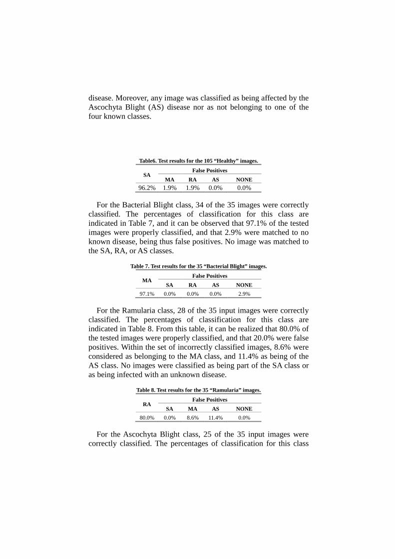
disease. Moreover, any image was classified as being affected by the Ascochyta Blight (AS) disease nor as not belonging to one of the four known classes.
Table6. Test results for the 105 “Healthy” images.
SA False Positives
MA RA AS NONE 96.2% 1.9% 1.9% 0.0% 0.0%
For the Bacterial Blight class, 34 of the 35 images were correctly
classified. The percentages of classification for this class are indicated in Table 7, and it can be observed that 97.1% of the tested images were properly classified, and that 2.9% were matched to no known disease, being thus false positives. No image was matched to the SA, RA, or AS classes.
Table 7. Test results for the 35 “Bacterial Blight” images.
MA False Positives
SA RA AS NONE 97.1% 0.0% 0.0% 0.0% 2.9%
For the Ramularia class, 28 of the 35 input images were correctly
classified. The percentages of classification for this class are indicated in Table 8. From this table, it can be realized that 80.0% of the tested images were properly classified, and that 20.0% were false positives. Within the set of incorrectly classified images, 8.6% were considered as belonging to the MA class, and 11.4% as being of the AS class. No images were classified as being part of the SA class or as being infected with an unknown disease.
Table 8. Test results for the 35 “Ramularia” images.
RA False Positives
SA MA AS NONE 80.0% 0.0% 8.6% 11.4% 0.0%
For the Ascochyta Blight class, 25 of the 35 input images were
correctly classified. The percentages of classification for this class
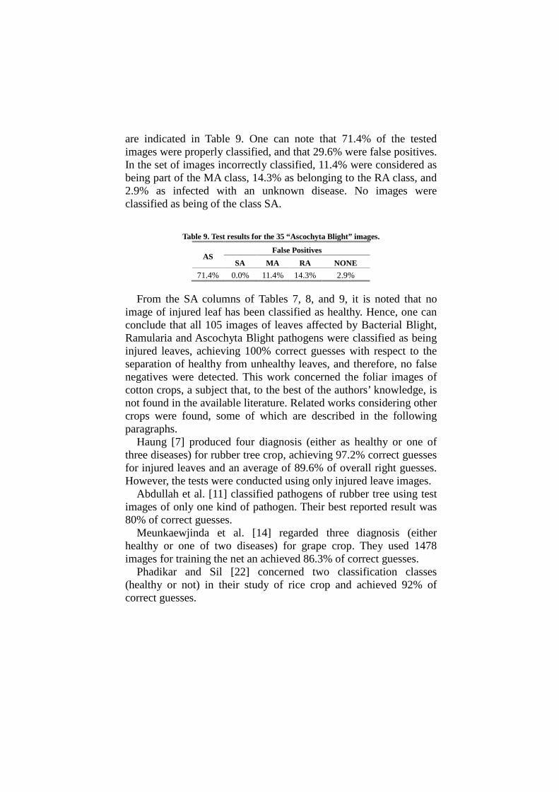
are indicated in Table 9. One can note that 71.4% of the tested images were properly classified, and that 29.6% were false positives. In the set of images incorrectly classified, 11.4% were considered as being part of the MA class, 14.3% as belonging to the RA class, and 2.9% as infected with an unknown disease. No images were classified as being of the class SA.
Table 9. Test results for the 35 “Ascochyta Blight” images.
AS False Positives
SA MA RA NONE 71.4% 0.0% 11.4% 14.3% 2.9%
From the SA columns of Tables 7, 8, and 9, it is noted that no
image of injured leaf has been classified as healthy. Hence, one can conclude that all 105 images of leaves affected by Bacterial Blight, Ramularia and Ascochyta Blight pathogens were classified as being injured leaves, achieving 100% correct guesses with respect to the separation of healthy from unhealthy leaves, and therefore, no false negatives were detected. This work concerned the foliar images of cotton crops, a subject that, to the best of the authors’ knowledge, is not found in the available literature. Related works considering other crops were found, some of which are described in the following paragraphs.
Haung [7] produced four diagnosis (either as healthy or one of three diseases) for rubber tree crop, achieving 97.2% correct guesses for injured leaves and an average of 89.6% of overall right guesses. However, the tests were conducted using only injured leave images.
Abdullah et al. [11] classified pathogens of rubber tree using test images of only one kind of pathogen. Their best reported result was 80% of correct guesses.
Meunkaewjinda et al. [14] regarded three diagnosis (either healthy or one of two diseases) for grape crop. They used 1478 images for training the net an achieved 86.3% of correct guesses.
Phadikar and Sil [22] concerned two classification classes (healthy or not) in their study of rice crop and achieved 92% of correct guesses.

4. Conclusions
The identification of pathogens in crops from their images is very important. However, it is also complex and difficult to achieve, mainly when the available image dataset is heterogeneous, containing images of different dimension, bright, contrast and resolution.
During the present work, a classification system was developed to automatically identify the existence or not of pathogens or foliar organs from images of cotton crops. Whenever no pathogens were found, the images were classified as healthy (SA). Otherwise, one of three pathogens was investigated, namely Ramularia (RA), Bacterial Blight (MA) and Ascochyta Blight (AS). Every time that an image was found not to be healthy and could not be classified as one of the three previously mentioned pathogens, it was classified as being infected by an unknown disease.
The highest difficulty of this work was to attain feature vectors that properly represented each class, because the available image dataset was very heterogeneous, as already mentioned. To solve this problem, the energy of the wavelet transform was computed from each sub-band obtained from the three-level decomposition of the original image. In order to find the best descriptor for each class, 108 feature vectors were built from the input image decomposition in channels R, G, B, H, S, V, I3A, I3B, and grey levels, using the wavelets Bey18, Coi12, Coi30, Dau4, Dau14, Dau34, Dau64, Dau76, Haar, Sym8, Sym16, and Vai24. These channels and wavelets were chosen for being widely reported as presenting adequate results in several applications [1, 3, 4, 7, 8, 15].
The feature vectors obtained were used for training the classification system. A Support Vector Machine (SVM) was used for classification as this technique has presented better results than other learning algorithms, such as Artificial Neural Networks. Supervised learning was used for training the SVM and a Gaussian function was used in the net mapping.
A total of 216 feature vectors was built, being 108 of which used to identify the best vector to represent the SA and LE classes, and the remainder 108 used to find the best representatives for the MA, RA, and AS classes. The best feature vectors found were then used in the final classification system, in which the classification was

achieved in a pipeline, being the original image initially classified as healthy or not, and those found to be unhealthy were then classified as MA, RA, AS, or neither of these classes. As such, the final classification achieved 96.2% of correct guesses for the SA class, 97.1% for the MA class, 80% for the RA class, and 71.4% for the AS class.
Considering the results of this work and those found in the available literature, it is possible to say that the approach developed appears to be quite promising, particularly taking into account the fact that a reduced number of samples was used in the SVM training. Besides, it can be concluded that the descriptors built properly represent each class, in spite of the heterogeneity of the presented image dataset, as they allowed an encouraging overall average of correct guesses around 89.5%.
5. References
[1] MOSHOU, Dimitrios; BRAVOA, Cédric; WESTB, Jonathan; WAHLENA, Stijn; MCCARTNEYB, Alastair; Ramona, Herman. Automatic detection of ‘yellow rust’ in wheat using reflectance measurements and neural networks; Computers and Electronics in Agriculture; v. 44, n. 3, p. 173-188, 2004.
[2] ZHANG, Yan-Cheng; MAO, Han-Ping; HU, Bo; LI, Ming-Xi; Features selection of cotton disease leaves image based on fuzzy feature selection techniques; International Conference on Wavelet Analysis, Beijing, China. v. 1, p. 124-129, 2007.
[3] SANYAL, P.;PATEL, S. C. Pattern recognition method to detect two diseases in rice plants; The Imaging Science Journal, v. 56, n. 6, p. 319-325, 2008.
[4] ANTHONYS, G.; WICKRAMARACHCHF, N. An Image Recognition System for Crop Disease Identification of Paddy fields in Sri Lanka; Fourth International Conference on Industrial and Information Systems, ICIIS 2009, Sri Lanka. p. 403-407, 2009.
[5] OTSU, Nobuyuki. A threshold selection method from gray-level histograms. IEEE Trans. Sys., Man., Cyber. v. 9, p. 62-66, 1979.
[6] NAKANO, Kazuhiro. Application of neural networks to the color grading of apples. Faculty of Agriculture, Niigata University, 2-8050 Ikarashi, Niigata 950-21, Japan, v. 18, p. 105-116, 1997.
[7] HUANG, K. Application of artificial neural network for detecting Phalaenopsis seedling diseases using color and texture features. Comput.Electron.Agric. v. 57, n. 1, p. 3-11, 2007.
[8] EL-HELLY, M.; EL-BELTAGY, S.; RAFEA, A. Image analysis based interface for diagnostic expert systems. In Proceedings of the Winter international Symposium on information and Communication Technologies.

ACM International Conference Proceeding Series, Cancun, México, Trinity College Dublin, v. 58, p. 1-6, 2004.
[9] YOUWEN, Tian; TIANLAI, Li; YAN, Niu; The Recognition of Cucumber Disease Based on Image Processing and Support Vector Machine; Congress on Image and Signal Processing, 2008, v. 2, p. 262 – 267, 2008.
[10] BOISSARD, P.; MARTIN, V.; MOISAN, S. A cognitive vision approach to early pest detection in greenhouse crops. Comput.Electron.Agric. v. 62, n. 2, p. 81-93, 2008.
[11] ABDULLAH, N.E.; RAHIM, A.A.; HASHIM, H.; KAMAL, M.M.; Classification of Rubber Tree Leaf Diseases Using Multilayer Perceptron Neural Network; Research and Development. SCOReD 5th Student Conference. p. 1-6, 2007.
[12] CUI, Di; ZHANG, Qin; LI, Minzan; ZHAO, Youfu; HARTMAN; Glen L. Detection of soybean rust using a multispectral image sensor, Sensing and Instrumentation for Food Quality and Safety, v. 3, n. 1, p. 49-56, 2009.
[13] WEIZHENG, S.; YACHUN, W.; ZHANLIANG, C.; HONGDA, W. Grading Method of Leaf Spot Disease Based on Image Processing. In Proceedings of the 2008 International Conference on Computer Science and Software Engineering. CSSE. IEEE Computer Society, Washington, DC, v. 06, p. 491-494, 2008.
[14] MEUNKAEWJINDA, A.; KUMSAWAT, P.; ATTAKITMONGCOL, K.; SRIKAEW, A.; Grape leaf disease detection from color imagery using hybrid intelligent system; Electrical Engineering/Electronics, Computer, Telecommunications and Information Technology, v. 1, p. 513-516, 2008.
[15] CAMARGO A., SMITH J.S. An image-processing based algorithm to automatically identify plant disease visual symptoms. Biosystems Engineering, v. 102 n. 1, p. 9-21, 2009.
[16] OHTA, Y.; KANADE, T., SAKAI, T. Color information for region segmentation. Computer Graphics and Image Processing. Department of Information Science, Kyoto, Japan, v. 13, n. 3, p. 222–241, 1980.
[17] FONSECA, E. ; GUIDO, R. C. ; SCALASSARA, P. R.; MACIEL, C. D. ; PEREIRA, J. C. Wavelet Time-frequency Analysis and Least-Squares Support Vector Machine for the Identification of Voice Disorders. Computers in Biology and Medicine, v. 37, n. 4, p. 571-578, 2007.
[18] YU, Z.; WONG, H.; WEN, G. A Modified Support Vector Machine and its Application to Image Segmentation. Image and Vision Computing, v. 29, p. 29-40, 2011.
[19] VAPNIK, V. Statistical Learning Theory. Springer Werlang: 2. ed., New York, 1998.
[20] SUASSUNA, N. D. Private Communication. Brazilian Company of Agricultural Research, Campina Grande, PB, Brazil.
[21] FI. Forestry Images.A joint project of the Center for Invasive Species and Ecosystem Health, USDA Forest Service and International Society of Arboriculture. The University of Georgia - Warnell School of Forestry and Natural Resources and College of Agricultural and Environmental Sciences. Available at: http://www.forestryimages.org (accessed in August 2010).

[22] PHADIKAR, Santanu; SIL, Jaya; Rice Disease Identification using Pattern Recognition Techniques; Proceedings of 11th International Conference on Computer and Information Technology (ICCIT 2008), Khulna, Bangladesh. p. 420-423, 2008.