ICES REPORT 14-28

August 2014

Compositional Flow Modeling Using a Multi-point FluxMixed Finite Element Method

by

Gurpreet Singh and Mary F. Wheeler

The Institute for Computational Engineering and SciencesThe University of Texas at AustinAustin, Texas 78712

Reference: Gurpreet Singh and Mary F. Wheeler, "Compositional Flow Modeling Using a Multi-point FluxMixed Finite Element Method," ICES REPORT 14-28, The Institute for Computational Engineering andSciences, The University of Texas at Austin, August 2014.

Compositional Flow Modeling Using a Multi-point Flux

Mixed Finite Element Method

Gurpreet Singh Mary F. Wheeler

August 21, 2014

Abstract

We present a general compositional formulation using multi-point flux mixed finiteelement (MFMFE) method on general hexahedral grids. The mixed finite elementframework allows for local mass conservation, accurate flux approximation and a moregeneral treatment of boundary conditions. The multi-point flux inherent in MFMFEscheme allows the usage of a full permeability tensor. The proposed formulation is anextension of single and two-phase flow formulations presented by Wheeler and Yotov(2006) with similar convergence properties. Further the formulation allows for blackoil, single-phase and multi-phase incompressible, slightly and fully compressible flowmodels utilizing the same design for different fluid systems. An accurate treatmentof diffusive/dispersive fluxes owing to additional velocity degrees of freedom is alsopresented. The applications areas of interest include gas flooding, CO2 sequestration,contaminant removal and groundwater remediation.

Keywords. compositional flow; multi-point flux; mixed finite element; general hexa-hedral grid

1 Introduction

Compositional flow modeling has been used for simulating CO2 sequestration, ground wa-ter remediation and contaminant plume migration. In the oil and gas industry it is widelyused for evaluating gas flooding scenarios as a tertiary recovery process. The gas floodingtargets achieving either direct miscibility or multi-contact miscibility to counter adversemobilities to maximize recovery. A number of variants of the above process exist, basedupon economical considerations, such as gas slug injection along with a chase fluid or wateralternating gas (WAG). The modeling involves solving a system of non-linear equations,invoking a local equilibrium assumption, including an equation of state. This combinedwith partial differential equations representing mass conservation represent a differentialalgebraic system which is known for its numerical difficulties. An extensive amount of liter-ature is available which elaborate on different model formulations and solution algorithmsto address this problem.

Some of the earliest expositions in compositional flow modeling were carried out byRoebuck et al. [1969] using a fully implicit solution scheme. Coats [1980] later presentedanother implicit formulation where the transmissibility terms (relative permeabilities) were

1

treated implicitly during the construction of Jacobian matrix. A similar formulation withexplicit transmissibility terms (relative permeabilities) was presented in Young and Stephen-son [1983]. These schemes were later categorized as primary variable switching (PVS) dueto change of primary variables associated with phase appearance and disappearance. Herea phase is assumed to be present only if the phase saturations lie between 0 and 1. A localcriteria based upon saturation pressure test is employed to test the stability of single phasegrid-blocks. Lauser et al. [2011] pointed out some of the issues which may arise due to pri-mary variable switching for near critical conditions. This was addressed by the latter usingnon-linear complimentarily condition defined such that negativity of phase-compositionsimply that the phase is not present.

A sequential solution scheme was presented by Acs et al. [1985] and Chang [1990] forsolving compositional flow equations. An implicit pressure equation, with explicit treatmentof transmissibility terms, is formed using volume balance assuming pore volume is equal tofluid volume. This is followed by an explicit concentration update. The approach was laternamed implicit pressure explicit concentration scheme on the lines of the well known implicitpressure explicit saturation (IMPES) scheme. Please note that the implicit or explicittreatment implies Newton iteration or time lagging terms to construct an approximationof the exact Jacobian. Watts [1986] also presented an extension of the IMPES scheme forcompositional flow following Acs et al. in the construction of a pressure equation basedupon a volume balance or constraint. Once the pressure equation is solved the total fluxesare evaluated. A system of implicit saturation equations are then solved with implicitsaturations. This is followed by phase flux evaluation and then component transport.

So far the sequential solution approaches discussed above march forward in time as-suming the pressure and saturation equations are decoupled. Sun and Firoozabadi [2009]discuss a coupled IMPEC scheme where iterations are performed between implicit pressureequation and explicit concentration updates, for a given time-step, until a desired toleranceis achieved. The implicit pressure and saturation equations are discretized using mixedfinite element (MFE) and higher-order, discontinuous-Galerkin (DG), respectively. In thiswork, we employ a similar iteratively coupled IMPEC solution scheme presented by Thomas[2009] while using a multi-point flux mixed finite element (MFMFE) method and lowest or-der DG for discretizing the pressure and saturation equations, respectively. This providesaccurate and locally mass conservative fluxes and eliminates grid orientation effects owing togradient in pressure. The MFMFE discretization also utilizes a full permeability tensor. Wealso differ in the use of a logically rectangular grid with general hexahedral elements. Theseelements lower the number of unknowns when compared to tetrahedral meshes. Further,the general hexahedral elements capture complex reservoir geometries without requiringsubstantial adjustment of associated petrophysical properties. This also allows for captur-ing of non-planar fractures Singh et al. [2014] as a future prospect for compositional flowmodeling in fractured poroelastic reservoirs.

It is also imperative to discuss some of the restrictions placed on phase-behavior mod-eling owing to a choice of solution algorithms discussed before. The Rachford-Rice (RR)Rachford and Rice [1952] equations allows a better treatment of the non-linearities presentedby the phase behavior model. The constant-K flash represented by RR equations can beeasily reformulated as a constrained optimization problem Michelsen [1994]. The objectivefunction for this minimization problem is known to be convex and therefore robust solu-

2

tion schemes can be utilized Okuno et al. [2010]. However, the model formulations used inLauser et al. [2011], Coats [1980] cannot take advantage of this due to the restrictive choiceof primary unknowns. Further, for implicit solution schemes, phase appearance and disap-pearance due to near critical fluid phase behavior poses significant problems. For primaryvariable switching (PVS) schemes this might introduce oscillations due to frequent changesin the rank of the Jacobian. Whereas, for complementarity condition based method theJacobian might become ill-conditioned or rank deficient. The IMPEC schemes circumventthese issues at the cost of relatively expensive but robust phase-behavior calculations.

In the sections below, we begin by describing the compositional model formulationalong with boundary, initial and closure conditions. This is followed by a description of thehydrocarbon phase behavior model based upon the local equilibrium assumption. Pleasenote that the aqueous phase is assumed to be slightly compressible. For the sake of brevity,we skip directly to the fully discrete formulation where a weak formulation of the problemis presented along with the associated finite element spaces and quadrature rules. We alsobriefly discuss the linearization choices leading to the construction of the implicit pressureequation. Finally, we present a number of numerical results comprising of verification andbenchmarking cases along with a comparison between TPFA (two-point flux approximation)and MFMFE schemes. A synthetic field case where gas flooding is used as a tertiary recoveryprocess further demonstrates the model capabilities for complex cases.

2 Compositional Model Formulation

We begin by describing a continuum description of the compositional model. The generalmass balance equation can be written in the differential form (also referred to as the strongform) and is given by Eqn. (1),

∂Wiα

∂t+∇ · Fiα −Riα − rmiα = 0. (1)

Where, Wiα is the concentration of component i in phase α, Fiα the flux of componenti in phase α, Riα the rate of generation/destruction of component i in phase α owing toreactive changes and rmiα the rate of increase/decrease component i in phase α owing tophase changes. The mass balance equation (1) can be expressed in an expanded form givenby,

∂(εαραξiα)

∂t+∇ · (ραξiαuα − εαDiα · ∇ (ραξiα)) = εαriα + rmiα. (2)

Here, εα it the volume occupied by phase α, ρα the density of phase α, ξiα the fractionof component i in phase α and Diα the dispersion tensor. Please note that the equationsoutlined in this section can have either a mass or molar basis. For the purpose of simplicity,a number of assumptions were made as stipulated below:

1. Rock-fluid interactions are neglected i.e., no sorption processes are considered.

2. Non-reactive flow.

Appying these assumptions to Eqn. (2), we obtain Eqn. (3).

∂(φSαραξiα)

∂t+∇ · (ραξiαuα − φSαDiα · ∇ (ραξiα)) = qiα + rmiα (3)

3

2.1 Component conservation equations

Summing eqn. (3) over the total number of phases (Np) and noting that∑

α rmiα = 0results in eqn. (4).

∂

∂t

(∑α

φSαραξiα

)+∇ ·

∑α

(ραξiαuα − φSαDiα · ∇ (ραξiα)) =∑α

qiα (4)

The phase fluxes (uα) are given by Darcy’s law,

uα = −K krαµα

(∇pα − ραg) . (5)

Here, Sα is the saturation of phase α (ratio of volume of phase α to pore volume), φ theporosity (ratio of pore volume to bulk volume), qiα the rate of injection of componenti in phase α (mass/mole/volume basis), and uα the Darcy flux of phase α. Also let,Ni =

∑α ραSαξiα and qi =

∑α qiα then the component conservation equations can be

written as,

∂

∂t(φNi) +∇ · Fi −∇ ·

(∑α

φSαDiα (∇ραξiα)

)= qi. (6)

We define component flux Fi as,

Fi = −K∑α

ραξiαkrαµα

(∇pα − ραg) , (7a)

Fi = −K

∑α

ραξiαkrαµα

(∇pref − ραg) +∑α 6=ref

ραξiαkrαµα∇pcα

. (7b)

2.2 Boundary and initial conditions

For the sake of convenience of model description we assume no flow external boundarycondition everywhere. However, this is by no means restrictive and more general boundaryconditions can be also be treated.

uα · n = 0 on ∂ΩN (8)

The initial condition is as follows,pref = p0, (9a)

Ni = N0i . (9b)

4

2.3 Closure and constraints

The phase saturations Sα are calculated as follows,

Sw =Nw

ρw,

So =(1− ν)

ρo

Nc∑i=2

Ni,

Sg =ν

ρg

Nc∑i=2

Ni.

(10)

Where, ν is the mole fraction of the hydrocarbon gas phase, and o, w and g represent thehydrocarbon oil, water and hydrocarbon gas phases, respectively. A saturation constraintexist on phase saturation given by, ∑

α

Sα = 1. (11)

The capillary pressure is a monotonic and continuous function of reference phase saturation(Sref). The relative permeabilities are continuous functions of reference phase saturation(Sref). A more general table based capillary pressure and relative permeability curve de-scription has also been implemented.

pcα = pα − pref (12)

Further, a slightly compressible and cubic equation of states are used for water and hydro-carbon phases, respectively.

ρw = ρw,0exp [Cw(pref + pcα − pref,0)] (13a)

ρα =pα

ZαRT, α 6= w (13b)

Here, ρα is the molar density of phase α including water. The porous rock matrix is assumedto be compressible, with Cr as the rock compressibility, satisfying the following relationship,

φ = φ0 [1 + Cr(pref − p0)] . (14)

3 Hydrocarbon Phase Behavior Model

The phase behavior modeling for hydrocarbon phases is based upon a local equilibriumassumption. The equilibrium component concentrations are then calculated point wisegiven a pressure (pref), temperature (T) and overall mole fraction (zi). A normalization ofcomponent concentrations Ni give overall component mole fractions zi.

zi =Ni∑Nci=2Ni

(15)

5

Let, ξiα be the mole fraction of component i in phase α and ν the normalized moles of gasphase, then from mass balance we have,

νξig + (1− ν)ξio = zi, (16a)

Nc∑i=2

ξio = 1, (16b)

Nc∑i=2

ξig = 1. (16c)

The partitioning coefficient Kpari of a component i between hydrocarbon phases is given by,

Kpari =

ξigξio. (17)

Rearranging the above equations we have,

ξio =zi

1 + (Kpari − 1)ν

, (18a)

ξig =Kpari zi

1 + (Kpari − 1)ν

. (18b)

The Rachford rice equation is given by,

f =

Nc∑i=2

(Kpari − 1)zi

1 + (Kpari − 1)ν

= 0. (19)

At equilibrium, the fugacities of a component i are equal in all the phases given by theiso-fugacity criteria (20).

g = ln(Φio)− ln(Φig)− lnKpari = 0. (20)

Where the fugacity of component i in phase α is given by,

ln(Φiα) = −Ci+BiBα

(Zα−1)−ln(Zα−Bα)− Aα

2√

2Bα

(2∑Nc

j=2 ξjαAij

Aα− BiBα

)ln

(Zα + (1 +

√2)Bα

Zα + (1−√

2)Bα

).

(21)For a given pressure (P ∗), temperature (T) and composition (~z) equations (19) and(20) canbe linearized in terms of lnKi and ν.(

∂f/∂lnKpar ∂f/∂ν∂g/∂lnKpar ∂g/∂ν

)(δlnKpar

δν

)=

(−R1

−R2

)(22)

Eliminating δν from the linear system,(∂f

∂lnKpar− ∂f

∂ν

(∂g

∂ν

)−1 ∂g

∂lnKpar

)δlnKpar = −R1 +

∂f

∂ν

(∂g

∂ν

)−1

R2. (23)

6

Since the system under consideration is highly non-linear with multiple solutions we musteither provide good initial guesses or constraint the system appropriately so as to get aunique solution. The phase behavior model relies upon providing a good initial estimatesfor lnKpar

i and consequently ν based upon heuristics. The Wilson’s equation (24) is anempirical correlation which provides initial guesses for Kpar

i s.

Kpari =

1

priexp

[5.37(1 + ωi)

(1− 1

Tri

)](24)

Using these partitioning coefficients (Kpari ) and the given composition (zi) equation (19)

is then solved to get an initial estimate for ν. We use three different ways of determiningphase stability and consequently the compositions of unstable phases using iso-fugacity flashcalculations. The three methods differ either in the calculation of initial estimates of Kpar

i sor the determination of phase stability (negative flash vs. tangent plane distance). However,the primary unknowns and equations for the three methodologies are the same as presentedin this section.

For non-polar molecules (hydrocarbon) Peng-Robinson cubic equation (47) of state em-pirically correlates pressure, temperature and molar volume. The values of Zα are calculatedusing this cubic equation of state, given in the appendix. For given pressure, temperature,composition (~n), partitioning coefficients ( ~Kpar) and vapor fraction (ν), the cubic equationof state provides three values of Zα. A unique solution is obtained by selecting the rootwhich has the minimum Gibb’s free energy given by,

∂G

∂ni

∣∣∣∣α,T,P

= µiα = µoi +RTlnΦiα, (25a)

dG|α,T,P =

Nc∑i=2

∂G

∂ni

∣∣∣∣α,T,P

dni = h(Zα). (25b)

Where µoi represents the reference state and is a different constant for each component.Amongst the three roots of the cubic EOS, Zα corresponding to the minimum dG|α,T,P ischosen. The cubic EOS, or alternatively Zα, is not a part of the Jacobian (Eqn. (22)) dueto the restriction placed by minimum Gibb’s free energy constraint. The algorithm for flashiteration can be outlined as follows:

1. Calculate an initial estimate of Kpari s from Wilson’s correlation (24).

2. For a given P, T, ~z and Kpari s calculated above, solve the Rachford-Rice equation (19)

for ν.

3. Calculate ξiα from (18).

4. Evaluate Zα using equation (47).

5. Evaluate residuals of fugacity equations (20), stop if convergence tolerance is achieved.

6. If tolerance is not achieved, solve (23) for new values of Kpari s.

7. Stop if Kpari is trivial i.e., Kpar

i = 1.

8. Return to 1.

7

4 Fully Discrete Formulation

We utilize a multi-point flux mixed finite element method to construct a fully discrete formof the flow problem describe earlier. Multi-point flux mixed finite element methods havebeen developed by Ingram et al. [2010], Wheeler and Yotov [2006] for general hexahedralgrids. Mixed finite element methods are preferred over other variational formulations due totheir local mass conservation and improved flux approximation properties. An appropriatechoice of mixed finite element spaces and degrees of freedom based upon the qudraturerule for numerical integration (Wheeler et al. [2011b], Wheeler and Xue [2011]) allow fluxdegrees of freedoms to be defined in terms of cell-centered gridblock pressures adajacent tothe vertex. A 9 and 27 point pressure stencil is formed for logically rectangular 2D and 3Dgrids, respectively.

4.1 Finite element spaces

Here we present the appropriate finite element spaces utilized to formulate an MFMFEscheme. An enhanced BDDF1 MFE space on E ,with additional degrees of freedom, for ageneral hexahedral element is defined on a reference unit cube Eqn.(28) by enhancing theBDDF1 space Eqn.(26). Let,V = v ∈ H(div; Ω) : v · n = 0 on ∂ΩN,W ≡ L2(Ω)

BDDF1(E) =P1(E)3 + r0curl(0, 0, xyz)T + r1curl(0, 0, xy

2)T + s0curl(xyz, 0, 0)T

+ s1curl(yz2, 0, 0)T + t0curl(0, xyz, 0)T + t1curl(0, x

2z, 0)T

=P1(E)3 + r0(xz,−yz, 0)T + r1(2xy,−y2, 0)T + s0(0, xy,−xz)T+

s1(0, 2yz,−z2)T + t0(−xy, 0, yz)T + t1(−x2, 0, 2xz)T

(26)

W (E) = P0(E) (27)

V ∗(E) =BDDF1(E) + r2curl(0, 0, x2z)T + r3curl(0, 0, x

2yz)T + s2curl(xy2, 0, 0)T

+ s3curl(xy2z, 0, 0)T + t2curl(0, yz

2, 0)T + t3curl(0, x2z, 0)T

=BDDF1(E) + r2(0,−2xz, 0)T + r3(x2z,−2xyz, 0)T + s2(0, 0,−2xy)T

+ s3(0, xy2,−2xyz)T + t2(−2yz, 0, 0)T + t3(−2xyz, 0, yz2)

(28)

The mixed finite element spaces on a physical element is mapped from a reference using thePiola and scalar transformations (29).

v ↔ v : v =1

JEDFE v F−1

E

w ↔ w : w = w F−1E

(29)

where FE denotes mapping from E to E; DFE and JE are the Jacobian and the determinantof FE , respectively. The discrete finite element spaces Vh and Wh on τh are given by,

Vh ≡ v ∈ V : v|E ↔ v, v ∈ V (E), ∀E ∈ τh,Wh ≡ w ∈W : v|E ↔ w, w ∈ w(E),∀E ∈ τh,

(30)

where H(div; Ω) ≡ v ∈ (L2(Ω))3 : ∇ · v ∈ L2(Ω).

8

4.2 Quadrature rule

For q, v ∈ V ∗h the local (on element E) and global (on domain Ω) quadrature rules aregiven by Eqn.(32),(31) and Eqn.(33), respectively. Where, Eqns.(31) and (32) give thesymmetrical and non-symmetrical quadrature rules. The non-symmetrical quadrature ruleshave been shown to have convergence properties for general hexahedra by Wheeler et al.[2011a].

(K−1q, v)Q,E =1

2d

2d∑i=1

JE(ri)(DF−1E )T (ri)DF

TE (ri)K

−1E (FE(ri))q(ri) · v(ri) (31)

(K−1q, v)Q,E =1

2d

2d∑i=1

JE(ri)(DF−1E )T (ri)DF

TE (rc,E)K−1

E q(ri) · v(ri) (32)

(K−1q, v)Q ≡∑E∈τh

(K−1q, v)Q,E (33)

Here, ri is the vertex of the reference element E, rc,E is the center of mass of E, KE is themean of K on E.

4.3 Weak formulation

We now consider the fully discrete variational formulation of the compositional flow model.The variables are taken at the most recent time iterate level everywhere except wheneverexplicitly indicated by index n. An iteratively coupled implicit pressure explicit concentra-tion (IMPEC) approach is used to solve equations in pressure (pref) and concentration (Ni)variables. The pressure and concentration equations are discretized in time using backwardand forward Euler schemes, respectively. Figure 1 shows a flow chart of the iterativelycoupled IMPEC scheme used in this work. The corresponding iterate level is representedby the index k. The discrete variational problem for reservoir pressure then reads: GivenNki,h ∈Wh, find F k+1

i,h ∈ Vh and pk+1ref,h ∈Wh such that,

⟨1

Λki,hK−1F k+1

i,h , vh

⟩Q,E

−(pk+1

ref,h,∇ · vh)E

= −∫∂E∩∂Ω

prefvh · n−

1

Λki,h

∑α6=ref

ρkα,hξkiα,hλ

kα,h∇pkcα,h, vh

E

+

(1

Λki,h

∑α

(ρ2α,h

)kξkiα,hg, vh

)E

,

(34)

(φk+1h Nk

i,h

∆t, wh

)E

+(∇ · F k+1

i,h , wh

)E−

(∇ ·

∑α

φk+1h Skα,hDiα,h · ∇

(ρkα,hξ

kiα,h

), wh

)E

=(qki,h, wh

)+

(φnNn

i

∆t, wh

)E

.

(35)

9

Here, k is used to represent iterate level for quantities which depend on both pressure andconcentrations such that pk+1

ref and Nki . The discrete variational problem for the concen-

tration update is: Given pk+1ref,h ∈ Wh, F k+1

i,h ∈ Vh and Nki,h ∈ Wh, find Nk+1

i,h ∈ Wh suchthat,(φk+1h Nk+1

i,h

∆t, wh

)E

+(∇ · F k+1

i,h , wh

)E−

(∇ ·

∑α

φk+1h Skα,hDiα,h · ∇

(ρkα,hξ

kiα,h

), wh

)E

=(qki,h, wh

)+

(φnNn

i

∆t, wh

)E

.

(36)Please note that a description of algebraic equations associated with the implicit pressure(Eqn. (35)) and explicit concentration (Eqn. (36)) systems is omitted to avoid redun-dancy. The reader is referred to earlier sections on compositional and phase behavior modelformulations for necessary relations.

Start

Pressure Solve

Tol < ϵYes

Time Step

No

Stop

n = n + 1

k = k + 1

Explicit Concentration Update

Figure 1: Iteratively coupled implicit pressure explicit concentration (IMPEC) scheme.

4.4 Treatment of diffusion/dispersion

The diffusion-dispersion tensor is the sum of molecular diffusion and hydrodynamic disper-sion given by:

Diα = Dmoliα +Dhyd

iα , (37a)

Dmoliα = ταdm,iαI, (37b)

Dhydiα = dt,α|uα|I + (dl,α − dt,α)uαu

Tα/|uα|. (37c)

10

Here τα is the tortuousity of phase α, dm,iα, dl,α, dt,α are the molecular, longitudinaland transverse dispersion coefficients, respectively. We define the diffusive/dispersive fluxas:

Jiα = φSαDiαρα · ∇ (ξiα) , (38)⟨1

φραSαD−1iα Jiα, vh

⟩Q,E

− (ξiα,∇ · vh)E = −∫∂E∩∂Ω

ξiαvh · n. (39)

The diffusion-dispersion tensor is evaluated locally for each corner-point similar to thepermeability tensor. The molecular diffusion (Dmol

iα ) is evaluated using cell-centered values

of dm,iα. Further, the hydrodynamic dispersion tensor (Dhydiα ) is calculated using the three

flux degrees of freedom associated with each corner-point.

4.5 Linearization

A Newton method is applied to form a linear system of equations followed by eliminationof component concentrations and fluxes resulting in a implicit pressure system. Once thepressures are evaluated an explicit update of Nc component concentrations is performed(IMPEC). The three phase saturations are calculated using equations (10) independently.Linearizing the above system of equations,⟨

1

Λi,hK−1δFi,h, vh

⟩Q,E

− (δpref,h,∇ · vh)E = −R3i, (40)

(φn+1,kh δNi,h

∆t, wh

)E

+

(Nn+1,ki,h

∆t

∂φ

∂pref,hδpref,h, wh

)E

+ (∇ · δFi,h, wh)E = −R4i. (41)

The local mass matrix and right hand side for component i can be written as,(Ai B 0BT Ci Di

) δFiδpref

δNi

=

(−R3i

−R4i

). (42)

We then eliminate δFi in favor of cell centered quantities δpref and δNi. The saturationconstraint, iso-fugacity criteria and RR equation can be linearized in terms of the unknownspref, Ni, K

pari and ν using equations (15) and (18) as,

∑α

∂Sα∂pref

δpref +∑α

∑i

∂Sα∂Ni

δNi+∑α

∑i

∂Sα∂lnKpar

i

δlnKpari +

∑α

∂Sα∂ν

δν = 1−∑α

Sα = −R5,

(43)Φiα = Φiα(pref, ξiα) = Φiα(pref, zi,K

pari ) = Φiα(pref, Ni,K

pari ), (44)

∂lnΦio

∂prefδpref +

Nc∑k=2

∂lnΦio

∂NkδNk +

Nc∑k=2

∂lnΦio

∂lnKpark

δlnKpark +

∂lnΦio

∂νδν −

(∂lnΦig

∂prefδpref

+

Nc∑k=2

∂lnΦig

∂NkδNk +

Nc∑k=2

∂lnΦig

∂lnKpark

δlnKpark +

∂lnΦig

∂νδν

)−∂lnKpar

i

∂lnKpark

δlnKpark = −R6i.

(45)

11

The above equations can also be written in the matrix form as,E F G HI J K L0 N O P

δpref

δNδlnKpar

δν

=

−R5

−R6

−R7

. (46)

We then construct the pressure equation by further eliminating δN and δlnKpar. Pleasenote that C contains contribution from ∂φ

∂prefand D contains ∂ρα

∂prefindirectly through N.

Eliminating δF , δN and δlnKpar from the above linear system of equations results in animplicit pressure system. Note that the diffusion is handled explicitly for both the implicitpressure solve and the concentration update. The values of phase compressibilities (Zα) areevaluated explicitly given pressure P, temperature T and component concentrations Nis.The derivatives of Zα with respect to P and Ni are therefore set to zero in the Jacobian.The Zα contribution is accounted for in the residual term. A more rigorous treatment wouldbe to expand the Jacobian in terms of Zα as well. However, the minimum Gibbs free energyconstraint (for a unique Zα) given by equation (25) is difficult to utilize.

5 Results

In this section, we present numerical experiments to verify and demonstrate the capabilitiesof MFMFE discretization scheme for compositional flow modeling. We begin with a verifi-cation case where a comparison is made between TPFA and MFMFE discretization schemesfor matching conditions. This is followed by another numerical experiment where we usea checker-board pattern permeability field to demonstrate better fluid front resolution forMFMFE scheme. Finally, we present a synthetic Frio field example where CH4 is injectedto achieve multi-contact miscible flooding.

5.1 Verification and benchmarking

Here we present a comparison between TPFA and MFMFE discretizations with a diagonalpermeability tensor. A quarter five spot pattern with 3 components (C1, C6 and C20) inaddition to the water component. Both the injection (bottom left corner) and production(top right corner, Figure 2) wells are bottom hole pressure specified with a pressure spec-ification of 1200 and 900 psi, respectively. The injection composition is kept constant at100% C1 with reservoir and grid block dimensions of 1000ft × 1000ft × 20ft and 20ft ×20ft × 20ft, respectively. The initial reservoir pressures and water saturations are 1000 psiand 0.2, respectively. A homogeneous, isotropic and diagonal permeability tensor field of50 mD was assumed with a homogeneous porosity field of 0.3. The temperature was keptconstant at 160 F. Figure 3 shows variation of component concentrations along the linejoining injector and producer for both TPFA and MFMFE discretizations. Please note thatsince the concentration profiles show a very good match the curves are not visible.

5.2 Checker-board pattern test

This numerical experiment demonstrates the differences in saturation profiles betweenMFMFE and TPFA discretization due to the use of a full permeability tensor. The reservoir

12

Figure 2: Oil saturation profile after 100 days using TPFA (left) and MFMFE (right)discretizations.

and fluid property information is kept the same as in the previous example differing onlyin permeability values. A checkerboard permeability field, as shown in figure 4 (left), istaken with values of 1mD (blue) and 100mD (red) to exaggerate the effects. Additionally,small off diagonal permeability values of 0.5mD were taken to construct a full permeabilitytensor for the MFMFE scheme. Figure 4 also shows the gas saturation profiles for the twodiscretization schemes after 500 days. It can be seen that the saturation profile on theleft has less jagged edges owing to the extended pressure stencil. The MFMFE scheme istherefore able to better resolve pressure and saturations at the fluid front.

Figure 4: Permeability field (left) and gas saturation profiles after 500 days for MFMFE(middle) and TPFA (right) discretizations.

5.3 Frio field test case

In this example, we present a synthetic field case using a section of Frio field geometryinformation to demonstrate some of the model capabilities. Note that the general hexahedralelements allows us to capture reservoir geometry accurately without requiring substantialchanges in the available petrophysical data. We consider six hydrocarbon components (C1,

13

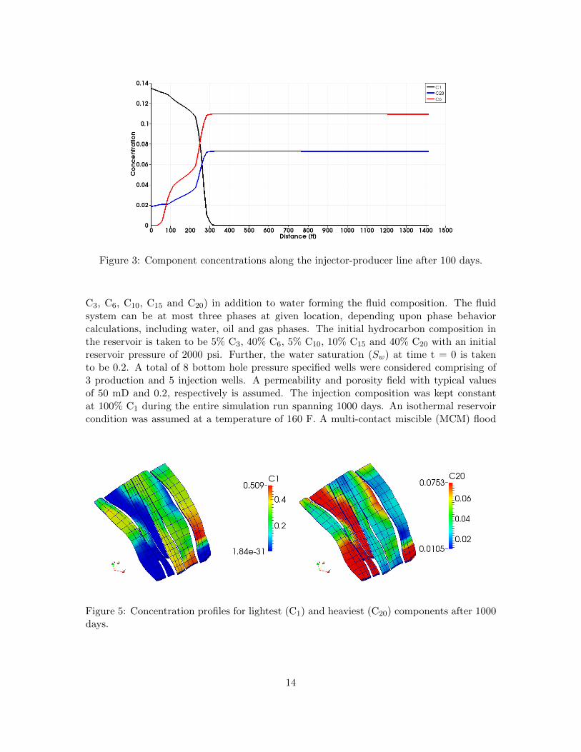
Figure 3: Component concentrations along the injector-producer line after 100 days.

C3, C6, C10, C15 and C20) in addition to water forming the fluid composition. The fluidsystem can be at most three phases at given location, depending upon phase behaviorcalculations, including water, oil and gas phases. The initial hydrocarbon composition inthe reservoir is taken to be 5% C3, 40% C6, 5% C10, 10% C15 and 40% C20 with an initialreservoir pressure of 2000 psi. Further, the water saturation (Sw) at time t = 0 is takento be 0.2. A total of 8 bottom hole pressure specified wells were considered comprising of3 production and 5 injection wells. A permeability and porosity field with typical valuesof 50 mD and 0.2, respectively is assumed. The injection composition was kept constantat 100% C1 during the entire simulation run spanning 1000 days. An isothermal reservoircondition was assumed at a temperature of 160 F. A multi-contact miscible (MCM) flood

Figure 5: Concentration profiles for lightest (C1) and heaviest (C20) components after 1000days.

14

is achieved at the given reservoir pressure and temperature conditions. Figure 5 showsthe concentration profiles for the lightest and heaviest hydrocarbon components after 1000days. Further, figure 6 shows the gas and oil saturation profiles after 1000 days.

Figure 6: Saturation profiles for gas (left) and oil (right) phases after 1000 days.

5.4 Brugge field CO2 flooding

In this example, we use CO2 gas flooding(Peters et al. [2009], Chen et al. [2010]) as the ter-tiary mechanism for recovering hydrocarbons. The distorted reservoir geometry is capturedusing 9×48×139 general hexahedral elements and then discretized using a MFMFE scheme.A constant temperature of 160 F is specified assuming an isothermal reservoir condition.The initial hydrocarbon composition is 40% (C6) and 60% (C20) with an initial reservoirpressure of 1500 psi.

Figure 7: Brugge field geometry with well locations.

An injected gas composition of 100% CO2 is further specified. Fig. shows the Bruggefield geometry with 30 bottom-hole pressure specified wells with 10 injectors at 3000 psi and

15

0.2 0.4 0.6 0.8 10

0.2

0.4

0.6

0.8

1

Sw

krw

,ro

krw

(Sw

)

kro

(Sw

)

0 0.2 0.4 0.6 0.8 10

0.2

0.4

0.6

0.8

1

Sg

krg

,ro

kro

(Sg)

krg

(Sg)

Figure 8: Water, oil and gas relative permeabilities.

0.2 0.4 0.6 0.8 10

5

10

15

20

25

30

So

Pc

go

0.2 0.4 0.6 0.8 10

5

10

15

20

25

30

35

40

45

Sw

Pc

ow

Figure 9: Capillary pressure curves.

20 producers at 1000 psi. The porous rock matrix is assumed to be water wet as reflected bythe relative permeability and capillary pressure curves in Figs. 8 and 9 ,respectively. Fig. 10shows the oil and gas saturation profile after 1000 days whereas Fig. 11 shows the pressuredistribution and concentration profiles for light (CO2), intermediate (C6) and heavy (C20)components. A multi-contact miscible flood is achieved with miscibility occurring at thetail end of the injected gas front.

Figure 10: Oil and gas saturation profiles after 1000 days.

16

Figure 11: Pressure and concentration profiles after 1000 days.

6 Conclusions

We developed a compositional flow model using MFMFE for spatial discretization. The useof general hexahedral grid leads to fewer number unknowns when compared to tetrahedralgrids and therefore lower computational costs. Further the discretization scheme allows suf-ficient flexibility in capturing complex reservoir geometries including non-planar interfaces.The hexahedra is a plausible choice for mesh elements since reservoir petrophysical data isusually available on similar elements. An MFMFE scheme therefore facilitates adaptationwith minimal changes to given information. Finally, the general compositional flow modelpresented here encompasses single, multi-phase and black oil flow models. This presentsa future prospect for multi-model capabilities where different flow models can be used inseparate reservoir domains.

7 Acknowledgements

The authors would like to express their gratitude towards Rick Dean (ConocoPhillips) forhis contributions to IPARS (Implicit Parallel Accurate Reservior Simulator) and valuableinputs.

References

Gabor Acs, Sandor Doleschall, and Eva Farkas. General purpose compositional model. OldSPE Journal, 25(4):543–553, 1985.

17

Yih-Bor Chang. Development and application of an equation of state compositional simu-lator, 1990.

C. Chen, Y. Wang, and G. Li. Closed-loop reservoir management on the brugge test case.Computational Geosciences, 14:691–703, 2010.

Keith Coats. An equation of state compositional model. Old SPE Journal, 20(5):363–376,1980.

Ross Ingram, Mary F Wheeler, and Ivan Yotov. A Multipoint Flux Mixed Finite ElementMethod on Hexahedra. SIAM Journal on Numerical Analysis, 48(4):1281–1312, January2010.

A Lauser, C Hager, R Helmig, and B Wohlmuth. A new approach for phase transitions inmiscible multi-phase flow in porous media. Advances in Water Resources, 34(8):957–966,2011.

M.L. Michelsen. Calculation of multiphase equilibrium. Computers & chemical engineering,18(7):545–550, July 1994.

R Okuno, R T Johns, and K Sepehrnoori. A New Algorithm for Rachford-Rice for Multi-phase Compositional Simulation. SPE Journal, 15(2):313–325, June 2010.

E. Peters, R. Arts, G. Brouwer, and C. Geel. Results of the Brugge benchmark study forflooding optimisation and history matching. SPE 119094-MS. SPE Reservoir SimulationSymposium, 2009.

H.H. Rachford and J.D. Rice. Procedure for Use of Electronic Digital Computers in Cal-culating Flash Vaporization Hydrocarbon Equilibrium. Transactions of the AmericanInstitute of Mining and Metallurgical Engineers, 195:327–328, 1952.

I F Roebuck, Jr, G E Henderson, Jim Douglas, Jr, and W T Ford. The compositionalreservoir simulator: case I-the linear model. Old SPE Journal, 9(01):115–130, 1969.

Gurpreet Singh, Gergina Pencheva, Kundan Kumar, Thomas Wick, Benjamin Ganis, andMary F Wheeler. Impact of Accurate Fractured Reservoir Flow Modeling on RecoveryPredictions. SPE Hydraulic Fracturing Technology Conference, 2014.

Shuyu Sun and Abbas Firoozabadi. Compositional Modeling in Three-Phase Flow for CO2and other Fluid Injections using Higher-Order Finite Element Methods. SPE AnnualTechnical Conference and Exhibition, 2009.

Sunil George Thomas. On some problems in the simulation of flow and transport throughporous media. 2009.

J W Watts. A compositional formulation of the pressure and saturation equations. SPEReservoir Engineering, 1(3):243–252, 1986.

18

M F Wheeler and Guangri Xue. Accurate locally conservative discretizations for modelingmultiphase flow in porous media on general hexahedra grids. Proceedings of the 12thEuropean Conference on the Mathematics of Oil Recovery-ECMOR XII, publisher EAGE,2011.

Mary Wheeler, Guangri Xue, and Ivan Yotov. A multipoint flux mixed finite elementmethod on distorted quadrilaterals and hexahedra. Numerische Mathematik, 121(1):165–204, November 2011a.

Mary F Wheeler and Ivan Yotov. A Multipoint Flux Mixed Finite Element Method. SIAMJournal on Numerical Analysis, 44(5):2082–2106, January 2006.

Mary F Wheeler, Guangri Xue, and Ivan Yotov. A Family of Multipoint Flux Mixed FiniteElement Methods for Elliptic Problems on General Grids. Procedia Computer Science, 4:918–927, January 2011b.

Larry Young and Robert Stephenson. A generalized compositional approach for reservoirsimulation. Old SPE Journal, 23(5):727–742, 1983.

8 Appendix

8.1 Peng-Robinson Cubic Equation of State

Z3α − (1−Bα)Z2

α +(Aα − 3B2

α − 2Bα)Zα −

(AαBα −B2

α −B3α

)= 0 (47a)

Zα = Zα − Cα (47b)

Aα =

Nc∑i=2

Nc∑j=2

ξiαξjαAij (47c)

Aij = (1− δij)(AiAj)0.5 (47d)

Ai = Ωoai

[1 +mi(1− T 0.5

ri )]2 priTri

2(47e)

Bα =

Nc∑i=2

ξiαBi (47f)

Cα =P ∗

RT

Nc∑i=2

ξiαci (47g)

Bi = Ωobi

priTri

(47h)

Ci =P ∗ciRT

(47i)

pri =P ∗

Pci(47j)

Tri =T

Tci(47k)

19

mi = 0.374640 + 1.54226ωi − 0.26992ω2i if ωi ≤ 0.49

= 0.379642 + 1.48502ωi = 0.164423ω2i + 0.0166663

i if ωi >0.49(48)

where,δij = Binary interaction parameters between component ‘i’ and ‘j’ (constant).pci = Critical pressure of component ‘i’ (constant).Tci = Critical temperature of component ‘i’ (constant).ωi = Accentric factor for component ‘i’ (constant, deviation of a molecule from beingspherical).Cα = Volume shift parameter (constant).Ωoa/bi = Constants corresponding to the equation of state.

Zα = Compressibility of phase ‘α’.

20