arX

iv:0

812.

1781

v1 [

astr

o-ph

] 9

Dec

200

8

Primordial Magnetic Fields in Cosmology

by

Iain A. Brown

THE THESIS IS SUBMITTED IN PARTIAL FULFILMENT OF THE REQUIREMENTS FOR THE AWARD OF

THE DEGREE OF

DOCTOR OFPHILOSOPHY

OF THE

UNIVERSITY OF PORTSMOUTH

March, 2006

Copyright

c© Copyright 2006 by Iain A. Brown. All rights reserved.

The copyright of this thesis rests with the Author. Copies (by any means) either in full, or of extracts,may not be made without the prior written consent from the Author.

ii

Abstract

Magnetic fields have been observed in galaxies, clusters of galaxies and probably in superclusters. Whilemechanisms exist to generate these in the late universe, it is possible that magnetic fields have existed sincevery early times. A field existing before the formation of thecosmic microwave background will leaveimprints from its impact on plasma physics that might soon beobservable. This thesis is concerned withinvestigating methods to predict the form of such imprints.

In chapter2 we review in detail a standard, linearised cosmology based on a Robertson-Walker metricand a universe filled with photons, massless neutrinos, colddark matter, a cosmological constant, andbaryons. We work in a synchronous gauge for ease of implementation in a Boltzmann code, and keep ourformalism general. We then consider the statistics of the cosmic microwave background radiation, assumingthat only scalar (density) perturbations cause significantimpact.

Chapter3 introduces an electromagnetic field of arbitrary size and presents the equations governing themagnetised cosmology, and the structure of the electromagnetic fields, in greater detail than has hithertobeen shown. We then invoke a hierarchy of approximations, treating the conductivity of the universe asinfinite and thus removing the electric field, and considering the energy density of the magnetic field to besmall. We present the resulting system in a computationallyuseful form and end by reviewing previousstudies into the damping scales induced by photon viscosity.

Chapter4 considers the intrinsic statistics of the magnetic stresses. We approach this issue in two ways.Analytical methods are exact but reliant on an underlying Gaussian distribution function for the magneticfield, and simulating fields on a finite grid allows a great freedom in the form of the field but imposes anundesirable granularity and an unphysical infra-red cut-off. We construct the two-point moments in Fourierspace, extending and improving the analytical results, some of which we present for the first time. There isexcellent agreement between the results from analysis and those from the simulated fields. At the one- andthree-point level we find significant intrinsic non-Gaussianities.

In chapter5 we turn to the observable impacts a primordial magnetic field. We briefly review previousstudies into constraints from the epoch of nucleosynthesisbefore turning to consider the cosmic microwavebackground. We briefly consider the potential impact of an evolving damping scale, which may causedecoherence in the sources. Assuming coherence, which is likely to be accurate for very infra-red fields,the statistics of the source can be mapped onto the cosmic microwave background in an extensible man-ner, modelling the source statistics and the photon evolution entirely seperately. We demonstrate that ourapproach is valid by reproducing the signals for Gaussian power law fields on the microwave sky. Afteroutlining how we will improve our predictions by employing aBoltzmann code, we show that it is a purelytechnical matter to extend the method to the three-point function. With detector sensitivity increasing, thenon-Gaussianity of the cosmic microwave background will bewell constrained in the near future and ourwork allows us to employ a new probe into the nature of an early-universe magnetic field.

iii

Preface

The work of this thesis was carried out at the Institute of Cosmology and Gravitation University of Portsmouth,United Kingdom.

The work in this thesis is based on work in collaboration withRobert Crittenden (ICG, Portsmouth).Much of chapter4 is based on the paper “Non-Gaussianity from Cosmic MagneticFields”, I. Brown and R.Crittenden, Phys. Rev.D72 063002 (2005).

I hereby declare that this thesis has not been submitted, either in the same or different form, to this orany other university for a degree, and that it represents my own work.

Iain Brown

iv

Acknowledgements

The work presented in this thesis could not have been performed without the help and collaboration ofmy supervisor, Robert Crittenden. One of the chapters of this thesis is based on and expanded from apaper written in collaboration with him. The support of the Institute of Cosmology and Gravitation, and inparticular of Prof. Roy Maartens, has also been invaluable,as have been discussions with Kishore Ananda,Chris Clarkson, David Wands, David Parkinson, Marco Bruni,Konstantinos Dimopoulos, Antony Lewisand others too numerable to mention. I must also thank my family for their support as writing the thesiswore on, and the patience and tolerance of my friends, particularly of Mike, Ricki, Laura, Emma, Chris andVivian. The largest thanks go to Kishore, Richard, Mat and Dan, who offered much appreciated hospitalityand sat through innumerable ”discussions” about the thesisand the state of the world, and to Kathryn, whorarely complained about the weight of emails and helped my sanity enormously. Thanks to them all, thiswas a lot less unpleasant than it might otherwise have been.

v

Table of Contents

Abstract iii

Preface iv

Acknowledgements v

1 Introduction 1

2 Standard Linearised FLRW Cosmology 62.1 The FLRW Geometry . . . . . . . . . . . . . . . . . . . . . . . . . . . . . . . . .. . . . 62.2 Fluid Matter . . . . . . . . . . . . . . . . . . . . . . . . . . . . . . . . . . . . .. . . . . 12

2.2.1 Generic Stress-Energy Tensor . . . . . . . . . . . . . . . . . . . .. . . . . . . . 122.2.2 Cold Dark Matter . . . . . . . . . . . . . . . . . . . . . . . . . . . . . . . .. . . 162.2.3 Single-Fluid Universes . . . . . . . . . . . . . . . . . . . . . . . . .. . . . . . . 16

2.3 Boltzmann Fluids . . . . . . . . . . . . . . . . . . . . . . . . . . . . . . . . .. . . . . . 182.3.1 General Boltzmann Fluids . . . . . . . . . . . . . . . . . . . . . . . .. . . . . . 182.3.2 The Photons . . . . . . . . . . . . . . . . . . . . . . . . . . . . . . . . . . . .. 242.3.3 E and B Modes . . . . . . . . . . . . . . . . . . . . . . . . . . . . . . . . . . . .342.3.4 The Line-of-Sight Approach . . . . . . . . . . . . . . . . . . . . . .. . . . . . . 342.3.5 The Neutrinos . . . . . . . . . . . . . . . . . . . . . . . . . . . . . . . . . .. . . 372.3.6 Truncation . . . . . . . . . . . . . . . . . . . . . . . . . . . . . . . . . . . .. . 38

2.4 Baryonic Matter . . . . . . . . . . . . . . . . . . . . . . . . . . . . . . . . . .. . . . . . 392.4.1 Tight-Coupling . . . . . . . . . . . . . . . . . . . . . . . . . . . . . . . .. . . . 40

2.5 Scalar Field Matter . . . . . . . . . . . . . . . . . . . . . . . . . . . . . . .. . . . . . . 422.6 The Evolution of the Universe . . . . . . . . . . . . . . . . . . . . . . .. . . . . . . . . 44

2.6.1 Periods in the Universal Evolution . . . . . . . . . . . . . . . .. . . . . . . . . . 442.6.2 Vacuum Domination – Inflation . . . . . . . . . . . . . . . . . . . . .. . . . . . 442.6.3 Radiation Domination . . . . . . . . . . . . . . . . . . . . . . . . . . .. . . . . 452.6.4 Matter-Radiation Equality . . . . . . . . . . . . . . . . . . . . . .. . . . . . . . 462.6.5 Matter Domination . . . . . . . . . . . . . . . . . . . . . . . . . . . . . .. . . . 472.6.6 Recombination – Formation of the CMB . . . . . . . . . . . . . . .. . . . . . . 482.6.7 Late-Time Acceleration . . . . . . . . . . . . . . . . . . . . . . . . .. . . . . . 48

2.7 The Cosmic Microwave Background . . . . . . . . . . . . . . . . . . . .. . . . . . . . . 492.7.1 The Sachs-Wolfe Equation . . . . . . . . . . . . . . . . . . . . . . . .. . . . . . 492.7.2 Statistical Measures on the Sky . . . . . . . . . . . . . . . . . . .. . . . . . . . 502.7.3 Temperature Auto-Correlation - Traditional Approach . . . . . . . . . . . . . . . 512.7.4 Angular Power Spectra from the Line-of-Sight Approach . . . . . . . . . . . . . . 532.7.5 The CMB Angular Power Spectrum . . . . . . . . . . . . . . . . . . . .. . . . . 55

3 Magnetised Cosmology 593.1 The Electromagnetic Field . . . . . . . . . . . . . . . . . . . . . . . . .. . . . . . . . . 59

3.1.1 Field and Stress-Energy Tensors . . . . . . . . . . . . . . . . . .. . . . . . . . . 593.1.2 Maxwell Equations and Stress-Energy Conservation . .. . . . . . . . . . . . . . 613.1.3 The Electromagnetic Field: Robertson-Walker and Bianchi Cosmologies . . . . . 62

3.2 Baryonic Matter: Cosmological Magnetohydrodynamics .. . . . . . . . . . . . . . . . . 633.2.1 Real Space . . . . . . . . . . . . . . . . . . . . . . . . . . . . . . . . . . . . .. 63

vi

3.2.2 Fourier Space . . . . . . . . . . . . . . . . . . . . . . . . . . . . . . . . . .. . . 663.3 Damping of Cosmological Magnetic Fields . . . . . . . . . . . . .. . . . . . . . . . . . 693.4 Conclusions . . . . . . . . . . . . . . . . . . . . . . . . . . . . . . . . . . . . .. . . . . 72

4 Statistics of Cosmic Magnetic Sources 734.1 Tangled Magnetic Fields . . . . . . . . . . . . . . . . . . . . . . . . . . .. . . . . . . . 73

4.1.1 Underlying Statistics of the Fields . . . . . . . . . . . . . . .. . . . . . . . . . . 744.1.2 Realisations of Magnetic Fields . . . . . . . . . . . . . . . . . .. . . . . . . . . 75

4.2 One-Point Moments . . . . . . . . . . . . . . . . . . . . . . . . . . . . . . . .. . . . . . 774.3 Two-Point Moments . . . . . . . . . . . . . . . . . . . . . . . . . . . . . . . .. . . . . 774.4 Three-Point Moments . . . . . . . . . . . . . . . . . . . . . . . . . . . . . .. . . . . . . 81

4.4.1 General Considerations . . . . . . . . . . . . . . . . . . . . . . . . .. . . . . . . 814.4.2 Scalar Bispectra . . . . . . . . . . . . . . . . . . . . . . . . . . . . . . .. . . . 824.4.3 Vector and Tensor Cross Bispectra . . . . . . . . . . . . . . . . .. . . . . . . . . 834.4.4 Tensor Auto-Correlation . . . . . . . . . . . . . . . . . . . . . . . .. . . . . . . 854.4.5 Results . . . . . . . . . . . . . . . . . . . . . . . . . . . . . . . . . . . . . . .. 86

4.5 The Lorentz Forces . . . . . . . . . . . . . . . . . . . . . . . . . . . . . . . .. . . . . . 884.6 A Damped Causal Field . . . . . . . . . . . . . . . . . . . . . . . . . . . . . .. . . . . . 894.7 Discussion and Conclusions . . . . . . . . . . . . . . . . . . . . . . . .. . . . . . . . . 90

5 Observable Impacts of a Magnetic Field 925.1 Overview . . . . . . . . . . . . . . . . . . . . . . . . . . . . . . . . . . . . . . . .. . . 925.2 Nucleosynthesis . . . . . . . . . . . . . . . . . . . . . . . . . . . . . . . . .. . . . . . . 93

5.2.1 Direct Bounds . . . . . . . . . . . . . . . . . . . . . . . . . . . . . . . . . .. . 935.2.2 Indirect Bounds . . . . . . . . . . . . . . . . . . . . . . . . . . . . . . . .. . . . 94

5.3 Large-Scale Magnetised Cosmology . . . . . . . . . . . . . . . . . .. . . . . . . . . . . 955.3.1 General Approach . . . . . . . . . . . . . . . . . . . . . . . . . . . . . . .. . . 955.3.2 Damping Scales . . . . . . . . . . . . . . . . . . . . . . . . . . . . . . . . .. . 965.3.3 Non-Equal Time Correlations . . . . . . . . . . . . . . . . . . . . .. . . . . . . 985.3.4 Vector Transfer Functions . . . . . . . . . . . . . . . . . . . . . . .. . . . . . . 995.3.5 Tensor Transfer Functions . . . . . . . . . . . . . . . . . . . . . . .. . . . . . . 101

5.4 CMB Power Spectra from Tangled Magnetic Fields . . . . . . . .. . . . . . . . . . . . . 1025.4.1 Analytical Estimates from the Literature . . . . . . . . . .. . . . . . . . . . . . . 1035.4.2 Numerical Estimates from the Literature . . . . . . . . . . .. . . . . . . . . . . . 1035.4.3 A New Approach to the Magnetised CMB Power Spectrum . . .. . . . . . . . . 1045.4.4 An Outline for Generating Statistics from CMBFast . . .. . . . . . . . . . . . . 108

5.5 The CMB Bispectrum . . . . . . . . . . . . . . . . . . . . . . . . . . . . . . . .. . . . . 1095.6 Conclusion . . . . . . . . . . . . . . . . . . . . . . . . . . . . . . . . . . . . . .. . . . 111

6 Discussion and Conclusions 113

A Further Issues in Perturbation Theory 116A.1 Derivation of the Robertson-Walker Metric . . . . . . . . . . .. . . . . . . . . . . . . . 116

A.1.1 Maximally-Symmetric Spaces . . . . . . . . . . . . . . . . . . . . .. . . . . . . 116A.1.2 The Robertson-Walker Metric . . . . . . . . . . . . . . . . . . . . .. . . . . . . 117

A.2 Perturbation Theory and Gauge Issues . . . . . . . . . . . . . . . .. . . . . . . . . . . . 119A.2.1 Metric-Based Perturbation Theory . . . . . . . . . . . . . . . .. . . . . . . . . . 120A.2.2 Synchronous Gauge . . . . . . . . . . . . . . . . . . . . . . . . . . . . . .. . . 123A.2.3 Poisson Gauge . . . . . . . . . . . . . . . . . . . . . . . . . . . . . . . . . .. . 123A.2.4 Transferral between Synchronous and Poisson Gauge . .. . . . . . . . . . . . . . 124A.2.5 Gauge Invariance and the Bardeen Variables . . . . . . . . .. . . . . . . . . . . . 124

B Viscous Fluids 126

C Vector and Tensor CMB Statistics 130C.1 Vector Contributions to the CMB in the Traditional Approach . . . . . . . . . . . . . . . . 130C.2 Tensor Contributions to the CMB in the Traditional Approach . . . . . . . . . . . . . . . 132

D E and B Modes 135D.1 Spin-Weighted Polarisation – E and B Modes . . . . . . . . . . . .. . . . . . . . . . . . 135D.2 The Line-of-Sight Approach . . . . . . . . . . . . . . . . . . . . . . . .. . . . . . . . . 138

D.2.1 Scalar Evolution . . . . . . . . . . . . . . . . . . . . . . . . . . . . . . .. . . . 139D.2.2 Vector Evolution . . . . . . . . . . . . . . . . . . . . . . . . . . . . . . .. . . . 139D.2.3 Tensor Evolution . . . . . . . . . . . . . . . . . . . . . . . . . . . . . . .. . . . 140D.2.4 Scalar CMB Angular Power Spectra . . . . . . . . . . . . . . . . . .. . . . . . . 140D.2.5 Vector and Tensor CMB Angular Power Spectra . . . . . . . . .. . . . . . . . . 142

E Supplementary Results concerning Source Statistics 143E.1 Magnetic Bispectra . . . . . . . . . . . . . . . . . . . . . . . . . . . . . . .. . . . . . . 143

E.1.1 Traceless Scalar-Tensor-Tensor Correlation . . . . . .. . . . . . . . . . . . . . . 143E.1.2 Vector-Tensor-Vector Correlation . . . . . . . . . . . . . . .. . . . . . . . . . . 144E.1.3 Tensor Auto-Correlation . . . . . . . . . . . . . . . . . . . . . . . .. . . . . . . 145

E.2 Geometry-Independent Large-Scale Results . . . . . . . . . .. . . . . . . . . . . . . . . 148

F The CMB Bispectrum 151F.1 The CMB Angular Bispectrum . . . . . . . . . . . . . . . . . . . . . . . . .. . . . . . . 151F.2 An Algorithm for EvaluatingJll′l′′ . . . . . . . . . . . . . . . . . . . . . . . . . . . . . .153

G Mathematical Relations 156G.1 Legendre Polynomials . . . . . . . . . . . . . . . . . . . . . . . . . . . . .. . . . . . . 156G.2 Spherical Harmonics . . . . . . . . . . . . . . . . . . . . . . . . . . . . . .. . . . . . . 157G.3 Bessel Functions . . . . . . . . . . . . . . . . . . . . . . . . . . . . . . . . .. . . . . . 157G.4 Exponential Expansions . . . . . . . . . . . . . . . . . . . . . . . . . . .. . . . . . . . . 158G.5 Miscellaneous . . . . . . . . . . . . . . . . . . . . . . . . . . . . . . . . . . .. . . . . . 158

H Conventions and Notation 159H.1 Conventions . . . . . . . . . . . . . . . . . . . . . . . . . . . . . . . . . . . . .. . . . . 159

H.1.1 Fundamental . . . . . . . . . . . . . . . . . . . . . . . . . . . . . . . . . . .. . 159H.1.2 Perturbation Theory . . . . . . . . . . . . . . . . . . . . . . . . . . . .. . . . . 159H.1.3 Magnetised Plasmas . . . . . . . . . . . . . . . . . . . . . . . . . . . . .. . . . 160

H.2 Notation . . . . . . . . . . . . . . . . . . . . . . . . . . . . . . . . . . . . . . . .. . . . 160

Chapter 1

Introduction

Magnetic fields are observed on many scales in the cosmos, from planetary scales with coherence lengthsof a few thousand kilometres and strengths of a few Gauss, to galactic scales with coherence lengths on theorder of kiloparsecs and a strength of approximatelyB ≈ µG. There are also fields with coherence lengthson the order of megaparsecs that lie between galaxies and have field strengths lying between nano- andmicro-Gauss; fields larger yet within clusters are also likely to exist, with field strengths of a comparablesize. While fields on supercluster scales are extraordinarily difficult to detect, there are suggestions thatfields up to the order of micro-Gauss may exist even there. (See for example [1, 2, 3, 4, 5, 6] for reviews.)It is no great leap to suggest that larger-scale fields yet maybe present and, if so, we require a means ofprobing them.

The three chief observational probes for astronomical fields are the Zeeman effect, synchotron radia-tion, and the Faraday rotation. The Zeeman effect, in which the uniform component of the magnetic fieldseparates molecular energy levels, is typically rather small (of the order of a few hertz for a micro-Gaussfield) and thermal effects can readily induce a greater splitting than this. For the strong fields found in manyastrophysical situations, the Zeeman effect can be a good probe; however, for fields on galactic scales andabove it is unlikely to be useful. Synchotron radiation is emitted from electrons spiralling around magneticfield lines; this allows one to estimate the total magnetic field transverse to the electron motion. Synchotronemission is very useful for detections of magnetic fields in external galaxies, but unfortunately the relativescarcity of free electrons in clusters and greater scales limits its use to galactic scales. Moreover while syn-chotron measurements are useful for determining the transverse field strength they do not give an estimateof the total field strength and are also rather model dependent. For larger-scale fields and to determine atotal field strength we resort to employing measures from Faraday rotation, in which a magnetic field rotatesthe plane of a light-beam’s polarisation. A Faraday rotation signal is readily detected from its strong fre-quency dependence. Even with the Faraday rotation, fields oncluster and supercluster scales are notoriouslydifficult to calculate with any certainty; estimates range from the nano-Gauss to micro-Gauss levels.

The origin of these fields remains uncertain; many of the mechanisms suggested to generate the ob-served fields require a pre-existing seed field and are more accurately dubbed “amplification” mechanismsthan generation mechanisms. For our purposes we separate creation and amplification mechanisms intoprocesses occurring before, during and after recombination.

Popular post-recombination processes include the dynamo mechanism [4, 7, 8] and the adiabatic com-pression of a previously-magnetised cloud [4, 9]. The dynamo mechanism occurs when a rotating galaxycontains a pre-existing, small, seed field. The vorticity induced by the galactic rotation then “winds up” themagnetic field lines, boosting the field strength on an astrophysical timescale, the extra magnetic energycoming from rotational kinetic energy. The dynamo mechanism can likely boost a seed field of the orderof 10−30 Gauss up to the observed level of around10−6 Gauss, although this efficiency is still a matterof some debate (see for example [8]). The adiabatic compression of a previously magnetised cloud is alsoeffective in boosting field strength; again one may visualise this as a compression of magnetic field lines,this time through an ever tighter packing rather than a tighter winding, and the extra magnetic energy comesfrom gravitational potential energy. Adiabatic compression is less efficient than is the dynamo mechanism;estimates are that a seed field of around10−20 Gauss is necessary to produce the observed fields on a re-alistic timescale. Of course, there is little reason to believe that both these processes cannot be operatingsimultaneously, with the compression of a rotating, magnetised cloud.

1

2 CHAPTER 1. INTRODUCTION

Neither of these mechanisms generate fields from scratch; westill require some initial genesis mecha-nism to explain the observed fields. This could conceivably occur within clusters and galaxies themselves,by some battery mechanism for example; [6] provides some coverage of traditional approaches (the “Bier-mann battery” for example) to this matter and [10, 11] are a few modern treatments of magnetic fieldsproduced in supernova batteries; such astrophysical sources do not here concern us. Instead we choose toconsider the possibility that the seed fields, or at least a significant component of them, were relics of anearlier era.

Mechanisms certainly exist to generate this field at reionisation [12, 13, 14] or at recombination itself[15, 16], and they might also have been created before recombination or even before nucleosynthesis.During the reionisation era magnetic fields can be created bythe “shadow” an overdensity casts in the fluxof an ionising source. While outside of the shadow an inducedelectric field is balanced by the radiationpressure, within the shadowed area the flux is weaker and the forces no longer balance; the ionised materialis then induced into motion and the resulting current produces a magnetic field. Such fields can be as largeas10−14 or even10−12 Gauss, and obey a power spectrumP ≈ kn−2 wheren is the spectral index of theoverdensities (assumed to be approximatelyn ≈ −1 in the realm of applicability [14]). These fields havecoherence lengths on the order of around1Mpc.

Fields originating at recombination will be relatively small-scale (though still large compared to galacticscales) and with strengths around10−20 Gauss. They are generated by current flows induced between elec-trons and ionised hydrogen and helium during recombinationby gravitational perturbations and radiationpressure.

There are many suggested mechanisms that can produce fields before recombination. One possibilityarises from certain inflationary theories. In general, the density perturbations and gravitational waves pro-duced during inflation are not conformally invariant, whilemagnetic fields are. Generating large-scale fieldsthen depends on breaking the conformal invariance of the magnetic field, with highly model-dependent re-sults. Possible generation mechanisms arise relatively naturally during the electroweak symmetry breakingphase, before or during inflation itself, or in a preheating stage; see for example [4, 6, 17, 18, 19, 20, 21, 22].Such fields have power spectra ranging fromP ∝ k to P ∝ k−1, or even further tilted to the red. Thesefields are often dubbed “acausal” since they are produced during or before inflation. It can be shown (e.g.[23]) that a field produced by a “causal” mechanism must have an indexn ≥ 2. There are also recentstudies into generic second-order phase transitions generating large-scale fields (e.g., [24, 25, 26, 27]);such fields generally have power spectra with an indexn ≈ 2, heavily modified by the complex physics.Cosmic defects, both those models from GUT theories and morerecent string-inspired models, might alsobe responsible [28, 29]; these fields are generated by vorticity induced by the self-interaction of a stringnetwork.

More recently, attention has been given to the possibility that magnetic fields might be created continu-ously in the period between lepton decoupling and recombination, through the vorticity naturally occurringat higher order in perturbation theory [30, 31, 32, 33]. Due to the nature of their production, such fields arenecessarily rather weak and small-scale, though adequate for sourcing cluster fields; they have a compli-cated power spectrum that goes ask2 for low k before damping away.

Dolgov [34] provides a brief overview of many creation mechanisms. It is also worth commenting that,after production, their nature could evolve in the very early universe, perhaps as a result of hydromagneticturbulence [35] or the inverse cascade [36, 37].

The exact magnetogenesis model is not our present focus; we are principally interested in studying theimpact a primordial magnetic field might have on cosmological perturbation theory and, more specifically,the cosmic microwave background. It is to be hoped that studying this field will allow constraints on thepossible strength of a primordial magnetic field – or, indeed, determine whether such a field is incompatiblewith observations. Research in this area is not new; studiesof magnetised universes of one form or anotherdate back at least to the 1960s (see for example [38, 39, 40]). However, in recent years much study has goneinto the development of a theory of cosmological magnetohydrodynamics.

Limits from nucleosynthesis can be particularly powerful,and applicable to tangled as well as large-scale magnetic fields [4, 5, 23]. The direct impact of a magnetic field, through the induced splitting inelectron energy levels and through the energy density it contributes to the universe can be used to constrainthe current field strength to the order of micro-Gauss. Thereis also an indirect bound arising from thegravitational waves generated by a magnetic field; Caprini and Durrer [23] demonstrate that the bounds onacausal fields generated in the extremely early universe areextraordinarily strong, to the level ofB ≈ 10−30

Gauss forn ≈ 0, and lessening only for strongly red spectra nearingn ≈ −3. These limits are not entirelyuncontested, however ([41, 42]).

3

The cosmic microwave background (hereafter CMB) provides additional tools for investigating theproperties of large-scale magnetic fields. Regardless of the time at which they were generated, all fieldscould be expected to leave a magnetised Sunyaev-Zel’dovicheffect (e.g. [43, 44]) and Faraday rotations ofthe primordial CMB [45, 46, 41]. Fields present before reionisation will impact on the physics of the era(e.g. [47]), and fields predating recombination will have a direct impact on the cosmological perturbationsproducing the primordial CMB [48, 49, 50, 51, 52, 53, 54, 55, 56, 57, 58, 59, 60, 61]. It is with the finalearly-time possibility that this thesis is concerned.

The field strength of early-time fields is already constrained by limits from the CMB. By assuming theuniverse to be of Bianchi type VII, Barrowet. al. [62] demonstrated that, assuming the total anisotropyallowed by the 4-year COBE results [63] to be due to a magnetic field, the field strength is constrainedto a current value ofB ≈ 10−9 Gauss. More recently, Clarksonet. al. [64] place weak limits on thestrength of the magnetic field by considering the impact on the CMB in a generic geometry; assuming aRobertson-Walker form tightens these bounds back to the order of nano-Gauss. It is worth stressing thatthese limits are for a large-scale, directional component to the field active on scales larger than the Hubblelength. Limits for a “tangled” configuration require a closer study.

Primordial magnetic fields can have a significant impact on the CMB. While early treatments focusedon the dynamics of a Bianchi universe [40, 65], more modern treatments [48, 49, 50, 51, 52, 53, 54, 55,56, 57, 58, 59, 60, 61, 66] consider either small perturbations around a large-scalehomogeneous field or atangled field configuration in which fields are taken to possess no net directionality above a certain scale,often associated with the cluster scale – that is, the orientation of the net cluster scale fields is random. Bothof these scenarios source CMB perturbations, directly through the scalar, vector and tensor stresses, andindirectly by the density and velocity perturbations they induce in the charged proton-electron fluids. Codefor calculating the vector and tensor anisotropies generated by primordial magnetic fields was recentlyadded to the publicly-available Boltzmann code CAMB [67, 59], and that for scalars has been modelledindependently [51, 60, 61].

Considering the dynamics of the magnetised cosmological plasma, Brandenburget. al. [35], Tsagas andBarrow [68], Jedamziket. al. [69] and Subramanian and Barrow [70] studied various aspects of magnetisedcosmological perturbation theory and in particular the damping of magnetosonic and Alfven waves withinthe magnetised cosmological fluid. They independently found that while fast magnetosonic waves undergoSilk damping in much the same way as standard acoustic waves,the slow magnetosonic and Alfven wavesare heavily overdamped and on some scales can survive Silk damping. This not only yields a power boostfor small scales of the CMB but could also have a strong impacton cluster formation.

Subramanian and Barrow [49, 53] make semi-analytical estimates of the impact of a stochastic tangledmagnetic field on the small-scale (l ≥ 1000) temperature perturbations on the CMB, extending this withSeshadri to the polarisation [54, 57]. They found that the Alfven waves generated by a tangled field of sizeB ≈ 10−9 Gauss can contribute a signal to the temperature angular power spectrum that begins to dominateat l ≈ 3000. The effect is more pronounced for bluer spectra. Durrer, Kahniashvili and collaborators (e.g.[50, 52, 55]) investigate the impact a tangled magnetic field would haveon the large-scale (l ≤ 500) CMBfor both temperature and polarisation angular power spectra. They find a similar decrease of signal for lown and that a field is constrained to be of the order of nano-Gaussif it has a spectral indexn ≈ −3, while acausal field withn ≈ 2 is even more tightly constrained. Numerical codes are naturally the most accurateand previous findings have been confirmed and enhanced for scalar modes by Koh and Lee [51], Giovannini[60] and Yamazakiet. al. [61], and for vector and tensor modes by Lewis [59].

The studies thus far have been limited to particular configurations of field statistics and power spectra.Even with the numerical models studied by Lewis, Koh and Lee and Yamazakiet. al. much reliance forthe primordial field’s power spectrum and statistics is placed on the results of Macket. al. [55]. Thislimits the study to a power-law power spectrum; while likelysufficient for fields produced by inflation, thisis unlikely to be accurate for more complex scenarios such asfields generated from phase transitions orplasma processes. Large-scale causal fields are restrictedto power spectran ≥ 2; due to the power that thisconcentrates on small scales, such spectra are unphysical without some additional cutoff or turnover. More-over the fields considered have been purely Gaussian and there is little reason to believe this to be a realisticassumption. Magnetogenesis mechanisms in the early universe tend to be exceptionally complicated and tomerely assume a resulting Gaussian field is not warranted. Indeed, one of the few mechanisms for whichthe statistical nature has been derived is the second-orderproduction of, for example, Matarreseet. al. [31]which, due to its nature, producesχ2 fields with a damped causal power spectrum.

Moreover, the results in Macket. al. and the work based on them is limited to the accuracy of theapproximations they employ for the damping scales, Alfvenvelocity and normalisation of the spectral

4 CHAPTER 1. INTRODUCTION

index. These approximations are again restricted to Gaussian power-law fields. Despite their efforts thereis also still not a fully unified treatment of magnetic fields in cosmology. While full treatments are providedin principle in Tsagas [71] or Tsagas and Maartens [72], resulting naturally from their use of the covariantand gauge-invariant approach to cosmology, Lewis’ application of this approach to CMB analysis [59]neglected the scalar modes. In a more traditional metric-perturbation approach to cosmology, Macket.al. [55] work in a gauge-invariant formalism and also neglect scalar modes. Koh and Lee [51] work in aconformal Newtonian gauge and thus consider only scalars. Giovannini [6], enhancing the study of Kohand Lee and seeking to fill the gaps in Lewis’ work, also employs conformal Newtonian gauge.

In this thesis we aim to review and extend the current research in this area, with a specific aim to-wards developing techniques by which a field with a significant tangled component could be constrainedby CMB observations, including contributions from the scalar, vector and tensor components in a fullyunified manner. In chapter2 we review in detail a linear-order cosmological perturbation theory of theclassical type pioneered by Lifshitz ([73, 74, 75]). We generally restrict ourselves to synchronous gauge forease of future integration with the CMBFast code [76]. In chapter3 we introduce the modifications to thestandard theory introduced by a magnetic field. Magnetic fields impact directly on the geometry throughthe magnetic energy density and isotropic pressure, but also through the anisotropic shear they introduce.Perhaps more importantly, however, the magnetic fields modify the conservation and Euler equations forthe baryons, making them into a cosmological equivalent of the classical MHD equations. The fields thensource slow magnetosonic waves and Alfven waves, both of which become heavily overdamped and can tosome measure survive Silk damping [70]. In the standard picture vector perturbations rapidly damp away(though Lewis has demonstrated that in principle a detectable signature might remain from primordial vec-tor modes sourced by the neutrino anisotropic stress after neutrino decoupling [77]); as with a system ofcosmic defects, however, the magnetic field provides an active source.

It appears increasingly likely from cosmological data suchas the CMB that the dominant source ofperturbations in the universe was adiabatic and Gaussian innature, consistent with the expectations of aninflationary universe [78, 79]. However, this does not exclude the possibility that non-linear sources –such as, but certainly not limited to, our magnetic fields – might also have played a role in generatingperturbations. While their impact on the power spectrum might be small, they could dominate any non-Gaussianities that we observe. In order to search for these optimally we need clear predictions for thenature of the non-Gaussian signals that they would source. In chapter4 we investigate in detail the intrinsicstatistics of an early-universe tangled magnetic field. Thestress-energy tensor of the magnetic field isquadratic and so at the very least we expect the energy density of the field to obey aχ2 distribution. To testthis suspicion, we analyse the intrinsic statistics of Gaussian-random magnetic fields, concentrating on thetwo- and three-point correlations between the scalar, vector and tensor components of the magnetic stresses.We do so by both generating realisations of Gaussian-randommagnetic fields and through numericallyintegrating pure analytical results, most of which are presented here for the first time. While the integrationswe present are reliant upon the fields being Gaussian-random, the code we use to generate our realisationsis easily extended to include any type of non-Gaussian seed field and any form of power spectrum, not justthe power-law typically considered. One motivating example is a field continuously sourced in the pre-recombination universe by the mechanism of, for example, Matarreseet. al. [31] which, being producedby the combination of two Gaussian fields, isχ2 in nature and which has a significantly non-trivial powerspectrum. As a first step towards considering this scenario,we model a Gaussian magnetic field with acausal power spectrum, exponentially damped on smaller scales. Unfortunately, the limited dynamic rangeof our realisations prevents us from directly modelling theend-result of the Matarreseet. al. mechanism;however, the field we consider will provide us with clues as toits nature.

The impact of magnetic fields on the CMB temperature and “gradient” E-mode polarisation angularpower spectra is likely to be relatively minor on the angularscales most easily resolved; they are expectedto begin to dominate at multipoles of aboutl ≈ 3000, which remains unprobed by WMAP and unlikely tobe detected with such accuracy for a long time yet, although measurements by the CBI, VSA (see e.g. [80]),ACBAR [81], Boomerang [82] and CAPMAP [83] probes are ever-improving, and the South Pole Telescope[84] is soon to come online. Moreover, angular scales this smallare likely to be heavily contaminated byforegrounds that will be extremely hard to remove without washing away the effects of a magnetic field.

The “rotational”B-mode of the CMB polarisation is relatively unexcited; in the standard modelB-modes are generated by gravitational waves produced by inflationary perturbations and by weak lensing,both with characteristic spectra. In general only vector and tensor perturbations excite theB-mode. Sincea magnetic field produces both of these we have, in principle,a clean probe for its properties. Moreover, acosmological magnetic field would naturally induce Faradayrotation in the CMB polarisation [85, 46, 45,

5

41], which would convert an amount of theE-modes generated by all three classes of perturbations intotheB-modes, in a characteristically frequency-dependant manner. In reality, unfortunately, a strong angularpower spectrum for theB-mode is a long way off.

In chapter5 we finally consider the observational impact of magnetic fields, briefly reviewing the knownconstraints from nucleosynthesis [5, 23] before turning in detail to the CMB temperature angular powerspectrum. Exploiting the simple time-evolution of a magnetic field we can tackle the issue from a slightlydifferent angle to previous authors, transferring the intrinsic magnetic statistics directly onto the CMB byintegrating them across magnetised transfer functions. This approach requires pre-computed power- orbi-spectra, which could naturally be either purely analytic or resulting from the realisations we generatedin chapter4. The transfer functions are derived entirely independently. The advantages of this approachare manifold. At the two-point level one might argue that theapproach of Subramanian and Barrow [53],Mack et. al. [55], Lewis [59] and Yamazakiet. al. [61, 66] is sufficient and a new formalism entirelyunnecessary. However, the techniques employed by these authors are restricted, both in the nature of thefields that it can model – only purely Gaussian, power-law fields – and in the heavy reliance on successiveapproximate solutions to a range of integrals. With our numerical approach, we are not at all restricted inthis manner and can consider a far wider range of magnetic fields and their imprint on the CMB angularpower spectrum. We consider the large-scale approximations to the magnetised transfer functions, whichthen enables us to demonstrate the validity of this approach. The extensibility is demonstrated using thedamped causal field we considered in chapter4.

Magnetic impacts on the two-point CMB spectra are likely to be subdominant to other sources untilvery small scales. An alternative probe comes from the non-Gaussianity that any magnetic field – includinga Gaussian field – will impart onto the CMB. From a large-scalemagnetic field, this non-Gaussianity wouldbe expected to show at relatively low multipoles. Given the quality of the current data at low mutipolesgenerated by the WMAP satellite and, in the near future, the Planck satellite, this would seem a sensibleapproach. Unfortunately, the analytical and semi-analytical approaches employed by, for example, Macket.al. and Subramanian and Barrow are unsuited to predictions for the CMB non-Gaussianity; the expressionsbecome rapidly unwieldy, albeit probably not insoluble. Weoutline briefly how our approach can instead beemployed to realistically predict the CMB angular bispectra arising from the various three-point correlationswe derived in chapter4. This approach shares its advantages – and disadvantages – with the two-point case.It is severely compromised by the limited dynamic range, more so even than the two-point correlations, dueto the strong mode-selection involved. Accurate intrinsicbispectra thus take a very long time and a largeamount of memory to produce since we must use the largest possible dynamic range and average manydifferent realisations. However, using such bispectra makes this approach highly extensible and the methodwe outline is entirely general. We conclude by outlining theprocedure by which we will generate CMBangular bispectra using transfer functions generated fromthe CMBFast Boltzmann code [86].

Chapter 2

Standard Linearised FLRW Cosmology

In this chapter we present a review, independently derived but, for the large part, recreating previously-known results, of the theory of linear cosmological perturbations of a Friedmann-Lemaıtre-Robertson-Walker universe. Sections believed original to this thesisinclude the discussions of vector perturbations.

2.1 The FLRW Geometry

Cosmological Spacetimes and the Robertson-Walker Metric

The Copernican principle states that the Earth is in no special part of the universe. If one assumes that theuniverse is isotropic about the Earth then applying the Copernican principle will immediately lead one toconclude that the universe is homogeneous and isotropic throughout. Perhaps the strongest evidence for anisotropic universe is the cosmic microwave background (CMB), which to a startling accuracy is observed topossess the same temperature (about2.728K) in all directions [78, 63]. Applying the Copernican principleleads us to conclude that the universe is isotropic around every point –i.e., homogeneous. We then expectthe metric modelling the present universe to be maximally-symmetric – that is, possessing the greatest pos-sible numbers of isometries or, equivalently, possessing the maximum number of Killing vectors. Clearlythis cannot be literally true, or we would not ourselves exist. However, if we consider the universe on a largeenough scale that the clumping of matter is entirely negligible, then it becomes a very reasonable assump-tion. We should note that these are indeed merely assumptions, and one can work with mildly anisotropiccosmologies and reproduce the observed microwave background (e.g. [87]) to within experimental error.Moreover, critics might point out that the direct observation of the CMB only makes a statement about theisotropy of the universe about the Earth; the homogeneous and isotropic universe follows only by declar-ing that isotropy complete and enforcing the Copernican principle. Non-homogeneous cosmologies arein general rather intractable, though there has been renewed work on the spherically-symmetric Lemaıtre-Tolman-Bondi metrics since some authors suggest such models may exhibit late-time acceleration withoutthe need for dark energy (see [88, 89, 90] for three recent, conflicting, viewpoints). We assume the Coper-nican principle to hold.

In appendixA we derive the Robertson-Walker metric by foliating spacetime with maximally-symmetricthree-spaces, and progress to a discussion of gauge issues in cosmology. Here we content ourselves withpresenting our metric ansatz, in a flat synchronous gauge. Weemploy the line element

ds2 = −dt2 + a2(t) (γij + hij) dxidxj = a2(η)

(

−dη2 + (γij + hij) dxidxj

)

. (2.1)

whereγij = diag(1, 1, 1) andhij is implicitly of order a small parameterε and includes contributionsfrom components transforming under co-ordinate maps as scalar, vector and tensor parts. The separationwill be performed in Fourier space. Synchronous gauge provides us with an unambiguous and familiartime co-ordinatex0 and, as long as we take care when specifying initial conditions to remove the spuriousgauge modes [91], is no worse than any other gauge choice for physical interpretation of results. Note thatan observer measures the proper time and co-ordinates,dt = dη/a anddri = dxi/a. We will generallyemploy the conformal timedη = dt/a, wherea(η) is the scale factor of the FLRW geometry, swapping toco-ordinate timet only in certain cases. We use the notationA = dA/dη andA′ = dA/dt for differentiation

6

2.1. THE FLRW GEOMETRY 7

of an objectA with respect to the conformal and co-ordinate times respectively, and employ an overbarAto denote background quantities andδA to denote perturbed quantities.

Basic Definitions

Consider a real-space covariant vectorBi, the 4-velocity, for example. Then the contravariant form will be

Bi = a−2γijBj ⇒(

aBi)

= γij(

a−1Bj)

and so one can define the comoving covariant vectorbi and its contravariant counterpart

bi = aBi, bi = a−1Bi, bi = γijbj .

In particular, this implies that∂i = γij∂j ,

wherexi is a comoving co-ordinate.Similarly, for a tensorBij ,

Bij = a−4γimγjnBmn ⇒(

a2Bij)

= γimγjn(

a−2Bmn)

leads to the definitions of the comoving tensorsbij andbij as

bij = a2Bij , bij = a−2Bij , bij = γimγjnbmn.

The mixed formbij is then simply

Bij = a−2γimBmj = γimbmj = bij .

The inverse metric [92] is

g00 = −a−2, g0i = 0, gij = a−2(

γij − hij)

which takes this form to retain the normality of the metric; the metric perturbation is a comoving tensor

hij = a−2δgij ,

and sohij = γimhmj = γijh

mj and hij = a2δgij = γimγjnhmn.

The scale factora is normalised today to unity,i.e. a0 = a(η0) = 1. This implies that comovingquantities become physical at the current epoch. The conformal timeη is then closely related to the Hubbledistance.1

Affine Connections and the Ricci Tensor

The affine connections in a metric space without torsion are the Christoffel symbols,

Γλµν =1

2gλκ (gµκ,ν + gνκ,µ − gµν,κ) .

For a perturbed Robertson-Walker metric these are

Γ000 = a

a ,Γi00 = 0Γ0i0 = 0

Γ0ij = a

a (γij + hij) + 12 hij

Γij0 = aaδij + 1

2 hij

Γijk = 12

(

∂khij + ∂jh

ik − ∂ihjk

)

.

(2.2)

1The equations derived in§2.2.3imply that if we assume the current acceleration to have started only recently, we can approximatethe current conformal time asη ≈ 2/H0 whereH0 is the current Hubble parameter.

8 CHAPTER 2. STANDARD LINEARISED FLRW COSMOLOGY

The Ricci tensor is then

Rµν = Rαµαν = Γαµν,α − Γαµα,ν + ΓαβαΓβµν − ΓαβνΓβµα.

Straightforward calculations then show that

a2R00 = 3

(

a

a−(

a

a

)2)

+1

2

(

h+a

ah

)

−2a2Ri0 = ∂ih− ∂j hij (2.3)

−a2Rij = −(

a

a+

(

a

a

)2)

δij −1

2hij −

a

ahij −

1

2

a

ahδij

+1

2

(

∂i∂jh+ ∇2hij − ∂k∂ihkj − ∂k∂jh

ik

)

.

Hereh = γijhij = hii is the trace of the perturbation and we have raised one of the indices.The Ricci scalar for this perturbed universe is then

R = Rµµ =1

a2

(

6a

a+ h+ 3

a

ah−∇2h+ ∂i∂

jhij

)

. (2.4)

This is in conformal time; were one to transfer back into co-ordinate time, one would find that the back-ground term becomes the more familiarR = 6

(

a′′/a+ a′2/a2)

.

The Einstein Equations

If one assumes only that the universe is composed of various fluids – effective (photons and neutrinos, forexample) and actual (baryons, CDM etc.), as well as other interacting or non-interacting components suchas electromagnetic fields or networks of cosmic defects – then one may express the matter content of theuniverse in a total stress-energy tensorT µν .

For intuitive purposes, this tensor can be defined in Minkowski space by

T 00 = −ρ, T i0 = −E i, T ij = P ij

whereρ is the mass/energy density of the matter component,Ei is the energy flux vector (which withc = 1is equivalent to the momentum density), andP ij is the momentum flux density (see [93]). A more rigorousdefinition of a general stress-energy tensor is presented later. The momentum flux density can be seperatedinto its trace and traceless parts by

T ij = pδij + Πij ⇒ 3p = T ii , Πi

j = T ij −1

3δijT

mm (2.5)

wherep is the isotropic pressure andΠij embodies the anisotropic stress and contains a traceless scalar

degree of freedom along with two vector and two tensor degrees of freedom. This vanishes for a perfectfluid, for which we have

T µν = (ρ+ p)uµuν + pδµν . (2.6)

The Einstein equations can be written

Gµν = Rµν − 1

2δµνR = 8πGT µν + Λgµν . (2.7)

Contracting these equations allows one to eliminate the Ricci scalar and express the Einstein equations inan alternative “trace-reversed” form,

Rµν = 8πG

(

T µν − 1

2δµν T

σσ

)

− Λδµν , (2.8)

2.1. THE FLRW GEOMETRY 9

which emphasises the vacuum equationsRµν = 0. There is obviously great redundancy amongst theseequations. At zeroth order, theG0

0 equation generates the Friedmann constraint equation and theGij equa-tion generates the Raychaudhuri evolution equation. At first order, theG0

0, Gi0 andRi0 generate constraintequations while theGij , R

00 andRij equations produce evolution equations. We shall select as evolution

equations theR00 for the scalar trace and theRij for the other components, and as constraints we shall select

G00 for the scalar trace andGi0 for the other components.

Employing the Ricci tensor and scalar (2.3– 2.4) found above, one readily finds that in the backgroundwe have

Friedmann; constraint, G00 : H2 =

(

a

a

)2

= −8πG

3

(

a2T0

0

)

+a2Λ

3, (2.9)

Raychaudhuri; evolution, δjiG

i

j : 2a

a−(

a

a

)2

= −8πG

3

(

a2Ti

i

)

+ a2Λ. (2.10)

whereH = aH is the Hubble factor in conformal time,H being the observable Hubble parameter. Thephysical meaning of these equations can be rapidly illustrated with the perfect fluid form of the stress-energytensor, for which we have

(

a

a

)2

=8πG

3a2

(

ρ+Λ

8πG

)

, 2a

a−(

a

a

)2

= −8πGa2

(

p− Λ

8πG

)

(2.11)

from which we may identify the cosmological constant as an effective perfect fluid with stress energy

T(Λ)µ

ν =Λ

8πGdiag (1,−1)

or, to phrase it differently, an unperturbed perfect fluid ofdensityρΛ = Λ/8πG and pressurepΛ = −ρΛ.Using the typical definition of a cosmological equation of statew = p/ρ we then havewΛ = −1.

The Friedmann equation can also be written as

1 =8πG

3H2a2ρ =

8πG

3H2ρ = Ω (2.12)

whereΩ is the ratio between the universe’s total energy density andthe critical density. For an individualspecies, then,

Ωi =8πG

3H2ρi,

∑

i

Ωi = 1. (2.13)

These are normally presented as observed during the currentera and the Friedmann equation can then bewritten

∑

i

Ωi0a−ni = 1 (2.14)

with the scale-factor embodying the time-evolution. It is seen later that for radiationni = 4, while formatterni = 3 and for a cosmological constantni = 0. Had we included a curvature term in our systemthen the effective energy density would evolve withni = 2.

The linearised equations are

Evolution, δR00 : h+

a

ah = 16πGa2

(

δT 00 − 1

2δT ii

)

,

Evolution, δRij : hij + 2

a

ahij +

a

ahδij −

(

∂i∂jh+ ∇2hij − ∂a∂jhia − ∂a∂

ihaj)

= 16πGa2

(

δT ij −1

2δijδT

σσ

)

,

Constraint, δG00 : 2

a

ah+ ∂j∂ih

ij −∇2h = −16πGa2δT 0

0 ,

Constraint, δGi0 : ∂j hij − ∂ih = 16πGa2δT i0.

10 CHAPTER 2. STANDARD LINEARISED FLRW COSMOLOGY

These equations are entirely generic; henceforth, however, the matter sources we shall consider willbe baryons, cold dark matter, photons, (massless) neutrinos, and in chapter3 an electromagnetic field.We could also add, for example, scalar fields and networks of cosmic defects. The explicit forms of thestress-energy tensor for the differing fluids employed in standard cosmology shall be considered in turn.

Fourier Space and the Scalar-Vector-Tensor Split

The system of equations presented above are most easily analysed by transferring them to Fourier spaceand separating the components into parts transforming as scalars, vectors and tensors under co-ordinatetransformations. We work with the Fourier convention

∂i → −ikki,

that is,

A(η,x) =

∫

A(η,k)e−ik.xd3k

(2π)3

for a scalar, vector or tensor quantityA. When necessary, co-ordinate axes will be aligned such thatx3 ‖ k.A vector quantity in this space can be separated into a scalarand a solenoidal part as

Bi = ikiBS +BiV , kiBiV = 0, (2.15)

with ki a comoving wavevector, which implies that

BS = −ikiBi, BiV = Bi − kikjBj =

(

δij − kikj

)

Bj = P ij (k)Bj , (2.16)

whereP ij (k) = δij − kikj is a projection operator projecting a quantity onto a hypersurface defined by theFourier modes. Likewise, a tensor quantity can be split into

Aij =1

3δijA+

(

kikj −1

3δij

)

AS +(

kiAVj + kjAiV

)

+AiTj , (2.17)

with the various conditionskiAVi = 0, kjAiTj = AiTi = 0,

whereA = Aii is the trace ofA, AS is the traceless scalar part ofA, AVi is the (divergenceless) vector partof A andAiTj is the (traceless, divergenceless) tensor part.

It is straightforward to demonstrate that the different components ofAij are then recovered by applyingvarious projection operators2 to the full tensor:

A = δjiAij ,

AS =3

2kj kiA

ij −

1

2A =

(

δji −3

2P ji (k)

)

Aij = Qji (k)Aij ,

AVi = kjAji − kikj k

kAjk = kjPki (k)Ajk = PkV

ij (k)Ajk(k), (2.18)

AiTj = Aij −1

3δijA−

(

kikj −1

3δij

)

AS −(

kiAVj + kjAiV)

=

(

P ia(k)P bj (k) − 1

2P ij (k)P ba (k)

)

Aab = P ibTja (k)Aab (k).

It is occasionally useful to work with fully symmetrised forms of the vector and tensor projection operators;when this is so we shall employPkVij = k(jP

k)i (k) as the vector projector to operate onT jk andP ibTja =

(

P i(a(k)Pb)j (k) − 1

2Pij (k)P ba (k)

)

for the tensors, where the curved brackets denote symmetrisation on the

2Technically onlyP ij (k) is a true projection operator since it obeysP i

i (k) = 2, P ij (k)P j

k(k) = P i

k(k). Any sensible definition

of a trace for the other projection operators vanishes; neither are they idempotent. However, we shall habitually referto them all asprojections.

2.1. THE FLRW GEOMETRY 11

enclosed indicesA(iBj) = (1/2)(AiBj+AjBi). We shall do this, for example, when we come to considerthe statistics of the magnetic field.

Separating the metric perturbation, one can see thathiTj will carry information about the gravitationalwaves whilehVi will carry information about vorticity.

We can now make identifications between our variables, separated using the above prescription, and theφ,B, Si, ψ, E, Fi, Gij employed in appendixA and by Mukhanov, Feldman and Brandenberger [94]. Sincewe are working in synchronous gauge the lapse and shift functions vanish, implyingφ = B = Si = 0; thespatial perturbation is, in the two notations,

−2ψγij + 2E,ij + 2F(i|j) +Gij = hij

which in Fourier space is

−2ψγij − 2k2kikjE − 2ikk(iFj) +Gij =1

3hγij +

(

kikj −1

3γij

)

hS + 2k(ihVj) + hTij

and so

ψ =1

6(hS − h), E = − 1

2k2hS , Fi =

i

khVi , Gij = hTij (2.19)

orh = −

(

2k2E + 6ψ)

, hS = −2k2E, hVi = −ikFi, hTij = Gij . (2.20)

In this representation of the gauge, then, the gauge-invariant Bardeen variables (A.37) are

2k2Φ = hS +a

ahS , 2k2Ψ =

a

ahS +

k2

3(hS − h) , kVi = ihVi . (2.21)

This is little more physically lucid than in the alternativeprescription and in this chapter we shall not employthe Bardeen variables though obviously we could rewrite thescalar and vector components of the Einsteinequations below as equations for them. We return to the vector Bardeen variable in chapter5.

Transferring the Einstein equations into Fourier space andseparating them across their scalar, vectorand tensor components (noting that theδRij equation contains a redundant scalar trace term, which weremove) leads us to

BackgroundEquations :

(

a

a

)2

= −8πG

3

(

a2T0

0

)

+a2Λ

3, 2

a

a−(

a

a

)2

= −8πG

3

(

a2Ti

i

)

+ a2Λ,

Scalar TraceEvolution : h+

a

ah = 8πGa2

(

δT 00 − δT ii

)

,

Traceless ScalarEvolution : hS + 2

a

ahS +

1

3k2 (h− hS) = 16πGa2δTS

VectorEvolution : hVi + 2

a

ahVi = 16πGa2δTVi , (2.22)

TensorEvolution : hiTj + 2

a

ahiTj + k2hiTj = 16πGa2δT iTj ,

ScalarConstraints :

a

ah+

1

3k2 (h− hS) = −8πGa2δT 0

0 , h− hS = 24πGa2

kδT

(i)S(0) ,

VectorConstraint : hiV = 16iπG

a2

kδT iV(0) .

with δTS, δTVi andδT iTj defined as above andδT i0 separated as

δT i0 = ikiδT(i)S(0) + δT iV(0) .

Here all the variables are now in Fourier space and are functions of conformal timeη only.We can then see that, in the absence of any source, the vector perturbations will damp away rapidly.

The tensor evolution equation is a damped wave equation and in the absence of tensor sources it will

12 CHAPTER 2. STANDARD LINEARISED FLRW COSMOLOGY

generate damped plane waves. Although vector perturbations are neglected in standard models, they mustbe considered in models containing active sources – models with networks of cosmic defects or magneticfields, for example. Inflation does, however, generate an amount of power in gravitational waves and sotensor modes are taken into account in the most accurate pictures. It is, however, a good approximation toconsider only scalar perturbations.

When these equations are studied for the separate components, it becomes necessary to discuss the baseswe are working in for the vectors and the tensors. These basesare introduced in section§2.3.2.

We now turn to the standard components of the matter/energy content: cold dark matter (§2.2.2), thephotons (§2.3.2), the massless neutrinos (§2.3.5) and the baryons (§2.4). We also consider, for brevity asbackground sources only, scalar field matter (§2.5) which can drive both inflationary and late-time acceler-ating phases. The electromagnetic field is discussed in chapter3.

2.2 Fluid Matter

2.2.1 Generic Stress-Energy Tensor

Cold dark matter and baryons are perhaps the simplest matterthat can be placed into the Einstein equations,especially if one neglects all viscous effects. Here we shall quote both shear and bulk viscosities and alsoheat conduction and their impacts on the stress-energy tensor; this will prove useful, for instance, whenmodelling photon viscosities. However when we consider thestandard cosmological sources of cold darkmatter (CDM) and baryons we shall neglect the imperfect elements.

To model imperfect fluids, seperate the stress-energy and particle current tensors into an ideal and anon-ideal part,

T µν = T (Ideal)µν + T (Non−Ideal)µ

ν = (ρ+ p)uµuν + pδµν + T (Non−Ideal)µν (2.23)

Nµ = Nµ(Ideal) +Nµ

(Non−Ideal) = nuµ +Nµ(Non−Ideal) (2.24)

whereρ is the fluid’s mass-energy density,p its pressure,n its number density anduµ its 4-velocity. Thisdecomposition introduces an ambiguity into the definitionsof ρ, p, n anduµ, so define

T 00 ≡ −ρ, N0 ≡ −n

in a comoving frame whereuµ = (1,0), andρ is the total energy density in this frame.p is defined as the“intrinsic” pressure when the non-ideal components vanish. The 4-velocity may be taken, as do Lifshitz andPitaevskii [93], to be the velocity of energy transfer (⇒ T 0i = 0 in a comoving frame), or it can be taken,as do Eckart [95] and Weinberg [96], to be the velocity of particle transport (⇒ N i = 0 in a comovingframe). We take Eckart and Weinberg’s definition.

These definitions imply thatT (Non−Ideal)00 ≡ 0,N0

(Non−Ideal) ≡ 0 andN i(Non−Ideal) ≡ 0 in a comoving

frame. Thus one can see that, in a comoving frame, the dissipative effects are held entirely within thestress-energy tensor; in a general frame,

Nµ(Non−Ideal) ≡ 0 (2.25)

uµuνT (Non−Ideal)µν = 0. (2.26)

An arbitrary stress-energy can then be found by finding the most generalT µν(Non−Ideal) allowed by both thisequation and by the second law of thermodynamics; for a demonstration see Weinberg [96].

The resulting stress-energy tensor of a generic barotropicfluid in an arbitrary frame is

T µν = ρuµuν + pHµν − χ (Hµαuν +Hα

ν uµ)Qα − ξHµαHνβW

βα − ζHµ

ν uα;α

= ρuµuν + pHµν + χµν + ξµν + ζµν

with a supplementary thermodynamic equation of state usually taken in cosmology to be of the barotropicand isentropic formp = w(ρ)ρ. Here the 4-velocity is

uµ =dxµ

d√−ds2

, (2.27)

2.2. FLUID MATTER 13

the projection tensor onto a hypersurface orthogonal touµ is

Hµν = δµν + uµuν,

the heat-flow vector is defined asQµ = Θ;µ + Θuµ;νu

ν , (2.28)

the shear tensor is defined as

Wµν = uµ;ν + u ;µ

ν − 2

3δµνu

α;α, (2.29)

andΘ is the temperature of the fluid.χ, ξ andζ are the (positive) coefficients of heat-flow, shear viscosityand bulk viscosity respectively3. For non-relativistic “dust” –i.e. non-relativistic, pressureless fluids, onethen takesw = 0. Both the baryons and the cold dark matter are taken to be non-relativistic since, even inthe presence of a primordial magnetic field, the baryons remain highly non-relativistic; see [62, 70, 64, 97].

This decomposition of the fluid stress-energy tensor is useful since it acts as a direct relativistic general-isation of the familiar components of the fluid stress-energy (see for example Landau and Lifshitz [93] andWeinberg [96]). An alternative is to decompose it according to the four-velocity of an observer; this is, forexample, employed in the gauge-invariant and covariant approach to cosmology [98, 99, 100], developedfrom covariant fluid mechanics [101, 102], wherein spacetime is decomposed into a3 + 1 split with theobserver’s four-velocity acting as a time parameter, and all tensorial objects are projected parallel to thevelocity and onto a hypersurface perpendicular to it. In this formalism, the stress-energy tensor splits intoTµν = ρuµuν + pHµν + qµuν + uµqν + πµν with qµ the momentum flux andπµν the anisotropic stress.This approach has many advantages but for the purposes of this thesis we shall retain the older, more famil-iar formalism. It should be noted, however, that the gauge-invariant and covariant approach has been usedwith great success in the field of magnetised cosmologies; see for example [68, 71, 72, 87, 103]. The greatbenefit of such an approach is that one formulates first the entirely non-linear equations and then curtailsthese to an approximation based around a Robertson-Walker background, as opposed to the metric-basedapproach we are employing wherein we set a (fictional) background metric and perturb up to a more re-alistic approximation. This then lets us draw qualitative conclusions about the non-linear behaviour of asystem; we can also find a clear physical interpretation of each term.

The two main thermodynamic properties of a fluid that we shallbe concerned with are the equation ofstate and the speed of sound, defined by

w =p

ρ, c2s =

∂p

∂ρ= w +

∂w

∂ρρ. (2.30)

and its temperature. We assume that the fluid is isentropic and barotropic, that is thatw = w(ρ). Theperfect fluid stress-energy tensor then has the components

T 00 = −ρ, T i0 = − (ρ+ p) vi, T ij = pδij ⇒ Πi

j = 0. (2.31)

We have not imposed any restrictions onw = w(ρ), which is implicitly a function of space and time. Toretain homogeneity,vi = O(ε) and so we neglect any second-order combinations ofvi and the metricperturbations. It is worth emphasising, however, that we have heavily restricted the physics of the fluidspecies we can consider; a more general fluid equation of state could involve termsp = w(ρ, S)ρ with Sthe entropy of the fluid, and a truly realistic equation of state would be of the formp = p(ρ, S) derivedfrom the micro-physics.

Expressing the temperature of the imperfect fluid as a background homogeneous component and aperturbation,4

Θ(x, η) = Θ(η) + δΘ(x, η),

and assuming that the viscosities can be treated as quantities of zeroth order inε, we can then find that, asone would expect, the energy flux is modified by both the heat conduction and also a drag from the bulk

3Note the change of notation from that usual in the fluid literature, as we are reservingη for the conformal time rather than theshear viscosity.

4While in this section we rigorously employ this notation, weshall in the future omit the overline on the background temperaturewhere the situation seems unambiguous.

14 CHAPTER 2. STANDARD LINEARISED FLRW COSMOLOGY

viscosity:

χi0 = χaΘ

(

vi +

(

a

a+

Θ

Θ

)

vi +∂iδΘ

Θ

)

, ζi0 = 3ζaa

avi (2.32)

while the stresses acquire contributions from the two viscosities,

ζij = −ζa(

3a

a+ ∇ · v +

1

2h

)

δij ,

ξij = −ξa(

∂ivj + ∂jvi + hij −

1

3δij

(

2∇ · v + h)

)

(2.33)

where we have scaled the coefficients of heat conductivity and bulk and shear viscosity byχa = χ/a andsimilar. Note that, as one should expect given our background, the heat conduction and shear viscosityare purely first-order inε. Were they to impact on the background they would impose a directionality onthe universe by, for example, a net heat flow or a net momentum.If we assume that a particle species iscollisionless then we can derive the temperature change from the first law of thermodynamics;

dQ =3

2d

(

p

ρ

)

+ pd

(

1

ρ

)

(2.34)

wheredQ is the change in heat andp the pressure. We can approximate the pressure asp = NΘ whereNis the particle number density (n = −3(a/a)n), the density asρ = Nm,m being the particle mass, and fora collisionless fluid setdQ = 0. With these substitutions we quickly see that

Θ + 2a

aΘ = 0 (2.35)

and so

Θ ∝ 1

a2. (2.36)

The background isotropic stress is, in full,

1

3T ii = p− 3ζa

a

a(2.37)

and so we see that, insofar as the background dynamics are concerned, the presence of a bulk viscosityserves to reduce the pressure of the universe.

For simplicity, we now assume that any fluids in the universe are perfect and derive their dynamics.Non-ideal fluids are considered in appendixB.

Real-Space Dynamics

The stress-energy conservation laws for the ideal part of this fluid are given by

T νµ;ν + T ν(I)µ;ν = Cµ,

whereT ν(I)µ is the summed stress-energy tensor of any interacting species (for example, the electromagneticfield will contribute an interaction term to the baryon fluid)andCµ is a collisional term providing a sourceor sink for stress-energy, a transfer of momentum between baryons and photons coupled by Thomsonscattering, for example. For clarity we shall always present the contributions to the continuity equations as−T ν0;ν. The interaction and non-ideal contributions add linearlyto the results of this section.

Evaluating the ideal fluid contribution, neglecting terms second order inh or vi but without yet linearis-ing thermodynamic properties yields

− T µ0;µ = ρ+ ∇ · ((ρ+ p)v) + (ρ+ p)

(

3a

a+

1

2h

)

, (2.38)

T νi;ν =∂ ((ρ+ p) vi)

∂η+ ∂ip+ 4

a

a(ρ+ p) vi − hji∂jp.

2.2. FLUID MATTER 15

Linearising the pressure will in general give

δp =∂p

∂ρδρ+

∂p

∂SδS

and so for an isentropic fluidδp = c2sρδ (2.39)

where we have linearised the density with a dimensionless perturbationδ = δρ/ρ with a spatial averagedensityρ – that is,ρ = ρ(1 + δ).

It is straightforward to now show that

ρ+ 3a

aρ (1 + w) = −C0,

∂ip = Ci (2.40)

for the background dynamics, and

δ + 3a

a

(

c 2s − w

)

δ + (1 + w)

(

∇.v +1

2h

)

= −δC0, (2.41)

vi +

(

w

1 + w+a

a(1 − 3w)

)

vi +c2s

1 + w∂iδ = δCi.

Fourier space

Transferring into Fourier space and separating across the scalar, vector and tensor components is generallystraightforward. Denoting the spatial trace of a tensorT ij asT = T ii , we quickly see that, for the idealsector of the stress-energy in the background,

T0

0 = −ρ, Ti

0 = 0, Ti

j = c2sρδij

and in the foreground,

δT 00 = −ρδ, δT i0 = −ρ (1 + w) vi, δT ij = c2sρδδ

ij .

We separate across the scalar, vector and tensor parts to get

T0

0 = −ρ, Ti

0 = 0, Ti

i = 3c2sρ, πij = 0

in the background and

δT 00 = −ρδ, δT

(i)S(0) = −ρ (1 + w) vS ,

δT iV(0) = −ρ (1 + w) vVi , δT = 3c2sρδ, δπij = 0.

The background matter conservation equation is

ρ+ 3a

aρ (1 + w) = −C0. (2.42)

At linear order, the ideal components are

δ + 3a

a

(

c 2s − w

)

δ + (1 + w)

(

kvS +1

2h

)

= −δC0, (2.43)

vS +

(

w

1 + w+a

a(1 − 3w)

)

vS − kc 2s

1 + wδ = δC(i)

S , (2.44)

viV +

(

w

1 + w+a

a(1 − 3w)

)

viV = δCiV . (2.45)

16 CHAPTER 2. STANDARD LINEARISED FLRW COSMOLOGY

2.2.2 Cold Dark Matter

Cold dark matter (CDM) is defined as a fluid that interacts withother species purely gravitationally, via theEinstein equations. Governing this fluid, in addition to theEinstein equations, will be the CDM specialisa-tion of the conservation laws (2.40, 2.41). “Cold” refers to the extreme non-relativistic nature of the darkmatter; one assumes that it has a vanishing equation of stateand speed of sound. Moreover, since CDMinteracts only gravitationally, it may be used to define the synchronous frame of reference; hence we setvic = 0 identically.

CDM then obviously has a background stress-energy tensor

T0

0 = −ρc, Ti

0 = Ti

i = Πi

j = 0 (2.46)

which contributes only an average density to the dynamics, and

δT 00 = −ρcδc, δT i0 = δT ii = δΠi

j = 0, (2.47)

in the foreground, with the CDM fluctuations providing potential wells that will seed the formation oflarge-scale baryonic structure. The stress-energy conservation equations become

ρc + 3a

aρc = 0, δc +

1

2h = 0. (2.48)

In the simplest model there are no viscous effects that can beassociated with cold dark matter; if therewere, it would by definition not remain “cold”. While naturally it would not take a particular leap ofintuition to envisage a bulk viscous material acting as CDM it is standard to instead reduce the fluid to itsvery barest fundamentals.

2.2.3 Single-Fluid Universes

An Ideal Fluid Universe

Consider a universe dominated by some generic perfect fluid with (constant) equation of statew and speedof soundc2s; this universe then evolves according to the (redundant) set of equations

ρ+ 3a

aρ(1 + w) = 0, H2 =

8πG

3a2ρ, 2

a

a−(

a

a

)2

= −8πGa2wρ. (2.49)

We differentiate the Friedmann equation to obtain an expression for ρ and substitute this back into theconservation equation, whence

2H(

H + (1 + 3w)H3)

= 0.

This has the trivial solutionH = 0, corresponding to an empty universe, and an ordinary differentialequation forH which we quickly solve for both the Hubble parameter and the scale factor to find

a = a0η2

1+3w , H =2

1 + 3w

1

η,

a

a=

2

1 + 3w

1 − 3w

1 + 3w

1

η2. (2.50)

The background density is best found by direct integration of the continuity equation, whence

ρ = ρ0

(a0

a

)3(1+w)

. (2.51)

We can then consider special cases of the equation of state:

• w = 1/3: A purely radiative or ultra-relativistic fluid has this equation of state, as demonstrated inthe next section. Withw = 1/3 we see that

a = a0η, H =1

η,

a

a= 0 (2.52)

2.2. FLUID MATTER 17

and so a radiative universe does not accelerate with respectto the conformal time, and the scalefactor grows linearly withη. The background density of the radiation fluid decays asa−4, which canbe interpreted as a stretching due to the volume expansion ofthe universe plus a stretching due tored-shifting.

• w = 0: A fluid with an effectively vanishing pressure is labelled “dust”; due to the extreme non-relativistic nature of their bulk distribution, baryons are assumed to be dust. Cold dark matter is alsotaken to be dusty. A dust-dominated universe evolves as

a = a0η2, H =

2

η,

a

a=

2

η2. (2.53)

The background density of dust evolves, as one might expect,with a−3 which is merely the volumeexpansion of the universe.

• w = −1/3: A fluid with such an equation of state causes (artificial) singularities to appear in theexpressions for the Hubble and acceleration parameters. Wewill consider the importance of this typeof fluid shortly.

• w = −1: As we saw earlier, a fluid with this equation of state behavesas a cosmological constant.The formalism above breaks down for a cosmological constantand we will consider it shortly.

In the light of the observations of distant type-Ia supernovae [104] implying the recent onset of anaccelerating epoch, we might also ask when the universe appears to undergo an accelerating expansion;demanding thata/a > 0 implies that the universe will expand for all fluids withw < 1/3. Thus allfluids from the critical radiative through non-relativistic and into negative pressure accelerate the universalexpansion with respect to conformal time. This is not, however, the physical acceleration observed by theastronomers as this is with respect to the conformal rather than proper time.

If we convert our system to co-ordinate timedt = a(η)dη, we can rewrite the Hubble and Raychaudhuriequations as

(

a′

a

)2

=8πG

3ρ,

(

a′′

a

)

= −8πG

6ρ(1 + 3w) (2.54)

with the matter continuity equation unchanged in form. We can immediately state from the Raychaudhuriequation that the universe will undergo accelerated expansion with respect to the observed co-ordinate timeif w < −1/3. Should there be a significant amount of a fluid with a lower equation of state than this thenthe universe will ultimately enter a period of never-endingaccelerated expansion.

If we repeat our analysis for co-ordinate time, withH again denoting the observed Hubble parameteranda′ the derivative of the scale factor with respect to time, we find that

a = a0t2

3(1+w) , H =2

3(1 + w)

1

t,

a′′

a= −2

9

(

1 + 3w

(1 + w)2

)

1

t2. (2.55)

• w = 1/3: For radiation,

a = a0

√t, H =

1

2t,

a′′

a= − 1

4t2(2.56)

and so the universe is manifestly undergoing deceleration during a radiation-dominated era.

• w = 0: For dust,

a = a0t2/3, H =

2

3t,

a′′

a= − 2

9t2. (2.57)

• w = −1/3: Here

a = a0t, H =1

t, a′′ = 0 (2.58)

and any fluid with a more negative equation of state will undergo an accelerating expansion. Accord-ing to this formalism the Hubble parameter will go singular for a cosmological constant and negativefor a fluid withw < −1.

18 CHAPTER 2. STANDARD LINEARISED FLRW COSMOLOGY

de Sitter Spaces

The casew = −1 cannot be analysed in the above way due to the vanishing ofρ. Instead we turn back tothe Hubble equation for a universe dominated by the constantterm; in conformal time this is

(

a

a

)2

= a2 Λ

3(2.59)

which has the unedifying solution

a(η) =

(

1

a1±√

Λ

3(η − η1)

)−1

(2.60)

wherea1 is the scale factor at some conformal timeη1. For Λ > 0 this is called de Sitter space, and forΛ < 0 it is anti-de Sitter space. This is not a very useful form for physical interpretation, and so we returnagain to co-ordinate time, wherein

(

a′

a

)2

=Λ

3(2.61)

with the more lucid solution

a(η) = a1e±√

Λ3 (t−t1), H = ±

√

Λ

3,

a′′

a=

Λ

3. (2.62)

de Sitter spaces are thus exponentially expanding or contracting spacetimes. Fluids with equations of statenearingw = −1 are quasi-de Sitter spacetimes; inflationary and quintessential models generate quasi-deSitter spaces from universes dominated by scalar fields of some sort. Any inflating model, not necessarilyof scalar fields, is characterised phenomenologically withw, and this can be found in the recent universefrom observations of distant supernovae, as well as from themicrowave background (wherein it is tangledin various degeneracies). Recently it was determined from large-scale structure with the observation of thebaryon oscillations in the galactic distribution. The current equation of state of the inflating component ofthe universe – whatever that may turn out to be – is entirely consistent with a cosmological constant, astested by groups analysing the WMAP+Supernovae datasets [78, 104] and recent detections of the baryonoscillations in the large-scale galactic structure [105, 106, 107].

2.3 Boltzmann Fluids

Here we will discuss a generic effective fluid governed by a Boltzmann equation. We then turn to considerin great detail a collisional photon fluid which exchanges energy-momentum with the baryon fluid, andfinally briefly consider massless neutrinos.

While the approach in this section is our own, the basic material is well-known and can be drawn fromvarious sources; see in particular Ma and Bertschinger [108] and Landriau and Shellard [109], along withPeebles [110, 111], Padmanabhan [112], Crittenden [113] and Crittendenet. al. [114, 115].

2.3.1 General Boltzmann Fluids

The Boltzmann Equation and Stress-Energy Tensors

Let us work initially in a Minkowski spacetime. Liouville’stheorem states that if a system is entirely satis-fied by a Lagrangian formulation with co-ordinatesxi and their conjugate momentaPi, then the distributionfunctionf defined by

dN = f(

xi, Pi, t)

d3xd3P (2.63)

wheredN is the number of particles in a volume element does not changein transport –i.e., df = 0. If onetakes the time derivative and includes a collisional term acting as a source or sink, the result is Boltzmann’sequation,

df

dt=∂f

∂t+∂f

∂xidxi

dt+

∂f

∂Pi

dPidt

=∂f

∂t+ vi

∂f

∂xi− ∂U

∂xi∂f

∂Pi= C[f ] (2.64)

2.3. BOLTZMANN FLUIDS 19

for some external 3-potentialU and some collisional termC[f ]. It is important to note that, since this arisesin a Lagrangian system,

vi, Pi

are variables canonical toxi.Given that the mass (or number), momentum and energy of particles are conserved in collisional pro-

cesses, we may state that∫

C[f ]d3P =

∫

m0C[f ]d3P =

∫

mC[f ]d3P =

∫

PiC[f ]d3P = 0

wherem2 = P 2 +m20 is the mass-energy of the particle concerned.

Now, it is clear that the number density of the distribution function is given at an event(x, t) by

N =

∫

fd3P

and so we immediately see that

ρ =

∫

mfd3P. (2.65)

It should also be clear that the average velocity of the system is given by

〈vi〉 =

∫

vifd3P∫

fd3p(2.66)

and that the average of two velocities is

〈vivj〉 =

∫

vivjfd3P

∫

fd3p. (2.67)

We can then immediately define the components of the stress-energy tensor (in Minkowski space) as

T 00 = −ρ = −

∫

mfd3p

T i0 = −E i = ρ〈vi〉 =

∫

mvifd3p (2.68)

T ij = P ij = ρ〈vivj〉 =

∫

mvivjfd3p.

Using these one may show that the various conservation conditions imply mass continuity,

∂ρ

∂t+

∂

∂xi(

ρ〈vi〉)

= 0, (2.69)

the Euler equation∂

∂t

(

ρ⟨

vi⟩)

+∂P ij∂xj

+ ρ∂U

∂xi= 0 (2.70)

and energy flow,∂

∂t(N 〈m〉) +

∂E i∂xi

+ ρ∂U

∂xi⟨

vi⟩

. (2.71)

The stress-energy tensor (2.68) is valid only in Minkowski space; however, we may define the mo-mentum four-tensorPµ = m0U

µ = m0dxµ/

√−ds2 and convert it to a tensorial expression valid in all

reference frames. In this way one may express a covariant stress-energy tensor of a Boltzmann fluid,

T µν =

∫ √−gd3PPµPνP 0

f (xµ, Pµ) . (2.72)

where the√−g is included to ensure normality of the integral.

In a non-trivial metric, one has to take care to differentiate between the momentumPµ appearing in thestress-energy tensor, canonical to the co-ordinatexµ, and the proper momentapµ measured in a Riemannian(locally-Minkowski) co-ordinate system (pµ = (m, pi), pµ = (−m, pi)). Clearly the canonical momentum

20 CHAPTER 2. STANDARD LINEARISED FLRW COSMOLOGY

Pµ is gauge-dependant, while the proper momentum,pµ is gauge-invariant. To link the two let us find thetransform between the FLRW frame and the comoving Riemannian frame.

Using the tensor transformation law to compare the two conjugate metrics,

gµν = a−2

(

−1 0

0 γij − hij

)

=∂xµ

∂xα∂xν

∂xβgαβ =

∂xµ

∂xα∂xν

∂xβdiag(−1, 1, 1, 1) (2.73)

one finds that∂x0

∂xα=

1

aδ0α,

∂xi

∂x0 = 0,∂xi

∂xj=

1

a

√

γij − 1

2hij (2.74)

to the first order inhij , and comparing the two metrics,

gµν = a2

(

−1 0

0 γij + hij

)

=∂xµ∂xα

∂xν∂xβ

gαβ =∂xµ∂xα

∂xν∂xβ

diag(−1, 1, 1, 1) (2.75)

gives∂x0

∂xα= aδα0 ,

∂xi∂x0

= 0,∂xi

∂xj= a

√

γij +1

2hij . (2.76)

Thus we can write the canonical momentum as

Pµ =1

a

(

m,

(

γij − 1

2hij)

pj

)

, Pµ = a

(

−m,(

γij +1

2hij

)

pj)

(2.77)

which satisfyPµ = gµνPν as one should hope. Taking the inner product of the four-momentum with itselfagain gives

PµPµ = −m20 = p2 −m2

as expected.We remove the explicit dependence ona by making a (non-canonical) transformation toǫ = am,

apj = qj = qnj whereni is the unit vector in the direction of the fluid’s momentum – that is, ǫ will bethe mass-energy measured by a comoving FLRW observer and we write the comoving momentum as anamplitude and a direction. Doing this gives us the canonicalmomentum

Pµ =

(

−ǫ, q(

γij +1

2hij

)

nj)

. (2.78)

and the taking the amplitude of this momentum gives

ǫ2 = q2 + a2m20. (2.79)

Working in polar co-ordinates in momentum space, the volumeelement is then

d3P =

(

1 +1

2h

)

q2dqdΩn

and we can rapidly calculate the determinant of the FLRW metric,

√−g = a−4

(

1 − 1

2h

)

.

We now perturb the distribution function around a homogeneous (thermal) background

f0(q) = gs

(

em/Θ0 ± 1)−1

wheregs – two, for both photons and neutrinos – is the statistical weight,Θ0 = aΘ is the temperature ofthe particles today, and where fermions take the positive sign and bosons take the negative sign. We writethe expansion as

f(

xi, q, nj, η)

= f0(q) + f0(q)f1(

xi, q, nj, η)

.

2.3. BOLTZMANN FLUIDS 21

Noting that∫

ninjdΩn =4π

3δij ,

∫

nidΩn =

∫

ninj nkdΩn = 0,

one can show that the linearised stress-energy components are

T 00 = −ρ = − 1

a4

∫∫

√

q2 + a2m20f0(1 + f1)q

2dqdΩn,

= −4π

a4

∫

√

q2 + a2m20f0q

2dq − 1

a4

∫∫

√

q2 + a2m20f0f1q

2dqdΩn, (2.80)

T i0 = − 1

a4

∫∫

q

(

ni +1

2njh

ij

)

f0(1 + f1)q2dqdΩn

= − 1

a4

∫∫

q2dqdΩqnif0f1, (2.81)

T ij =1

a4

∫∫

q2nanb(

γia − 12h

ia) (

γjb + 12hjb

)

√

q2 + a2m20

f0(1 + f1)q2dqdΩn

=4π

3a4δij

∫

q2f0√

q2 + a2m20

q2dq +1

a4

∫∫

q2√

q2 + a2m20

ninjf0f1q2dqdΩn. (2.82)

For massless particles, such as the photons and neutrinos weconsider, we can setm0 = 0 in the aboveequations which reduce to

−T 0

0 = Ti

i =4π

a4

∫

qf0q2dq, T

i

0 = 0, Πi

j = 0 (2.83)

in the background, and

− δT 00 = δT ii =

1

a4

∫∫

qf0f1q2dqdΩn,

δT i0 = − 1

a4

∫∫

qnif0f1q2dqdΩn, (2.84)

δΠij =

1

a4

∫∫

qf0f1

(

ninj −1

3δij

)

q2dqdΩn (2.85)

for the perturbations.A massless Boltzmann fluid – corresponding to a collection ofphotons or massless neutrinos, or to

an extremely relativistic fluid – then behaves to zeroth order as a barotropic perfect fluid with equation ofstatep = 1

3ρ, as we previously stated. While this equation of state also holds in the foreground, the extantanisotropic stresses ensure that the effective fluid is far from perfect.

Returning to the Boltzmann equation (for a species not necessarily massless), we may now write it interms of our new variables as

f0∂f1∂η

+ f0dxi

dη

∂f1∂xi

+dq

dη

∂f0∂q

+ f0dq

dη

∂f1∂q

+ f1dq

dη

∂f0∂q

+ f0dnidη

∂f1∂ni

= C[f ]. (2.86)

In this expression, the only quantities of unknown order aredq/dη anddni/dη. If we consider the geodesicequation

P 0 dPµ

dη= −ΓµαβP

αP β

where√−ds2 = dη since we are considering particles along their worldlines,then the time component will

yield

εdε

dη=a

a

(

ε2 − q2)

− 1

2q2ninj h

ij

which, on substituting for the mass-energy relation, gives

qdq

dη=a

a

(

ε2 − q2 − a2m20

)

− 1

2q2ninj h

ij

22 CHAPTER 2. STANDARD LINEARISED FLRW COSMOLOGY

and sodq

dη= −1

2qninj h

ij . (2.87)

Similarly, considering the space component will give

2dni

dη= ninmnnh

mn − nj hij − 2q

εnmnn∂

mhin +q

εnmnn∂

ihmn ≈ O(h). (2.88)

We may also writedxi/dη ≈ (q/ε)ni to zeroth order.The Boltzmann equation then becomes in Fourier space

f0∂f1∂η

− ikq

εkin

if0f1 −1

2qninj h

ij ∂f0∂q

= C[f ]

to the first order. Dividing through by the background distribution function and settingm0 = 0 we finallyhave, defining the angle cosineµ = k.n,

∂f1∂η

− ikµf1 −1

2qninj h

ij ∂ ln f0∂ ln q

=C[f ]

f0. (2.89)

Brightness Functions

The “brightness” function of a Boltzmann fluid can be looselyseen as an analogue of the fractional densityperturbation and is defined by

F(

ki, ni, η)

=

∫

q2dqf0f1q∫

q2dqf0q(2.90)

One can then see that the exact analogue of the fractional density perturbation,

δ =δρ

ρ=

∫

q2dqdΩqf1f0∫

q2dqdΩqf0=

1

4π

∫

dΩF

sincef0 has no angular dependence. One can then see the brightness function as the density contrast withinsome small solid angle.

It proves useful to expand the brightness function over the Legendre polynomials with

F (k, n, η) =

∞∑

l=0

(−i)l (2l + 1)Fl (k, η)Pl (µ) . (2.91)

The usefulness of this expansion is that the moments of the brightness function are then recovered by

Fl(k, η) =(−i)−l

4π

∫

dΩPl(µ)F (k, n, η),

and one sees that the zeroth moment is the density and the firstmoment is related to the velocity. Ignoringthe possibility of vector and tensor perturbations for the moment, one can write

δ = F0, vS = −3i

4F1. (2.92)

Curtailing the Legendre expansion at the first order will then give a rough approximation to the brightnessfunction which is occasionally useful,

F ≈ δ + 4µvs. (2.93)

To express the Boltzmann equation in terms of the brightnessfunction it is easiest to relate the per-turbation to the distribution function with the brightnessfunction. Using the relation between a masslessparticle’s density and temperature,

δρ

ρ= 4

δΘ

Θ

2.3. BOLTZMANN FLUIDS 23

one may write the distribution function as the background function with a temperature perturbation,

f = 2

(

exp

(

q

Θ0(1 + 14F )

)

− 1

)−1

.

SinceF is a fully arbitrary function this retains the full generality of the distribution function. Expandingthe exponentials using the binomial expansions one may now see that

f1 = F

(

q

4Θ0

exp(q/Θ0)

exp(q/Θ0) − 1

)

.

Using the form off0 we may now see that this is identical to

f1 = −1

4

∂(ln f0)

∂(ln q)F. (2.94)

The Boltzmann equation, expressed in terms of the brightness function, then becomes

∂F

∂η− ikµF + 2ninj h

ij = C [F ] , (2.95)

where

C [F ] = − 4

f0

(

∂ (ln f0)

∂ (ln q)

)−1

C[f ].

Written in terms of the brightness function, the stress energy tensor is

δT 00

ρ=

δT iiρ

= − 1

4π

∫

dΩnF = −δ,

δT i0ρ

= − 1

4π

∫

dΩnniF = −4

3vi, (2.96)

δT ijρ

=1

4π

∫

dΩnninjF = Πi

j

with the solid angledΩn = sin θdθdφ andθ andφ are defined in a co-ordinate system withx3 ‖ n. Wemay separate the energy flux and momentum flux density into scalar, vector and tensor parts as

δT(i)S(0)

ρ=

i

4π

∫

dΩnµF,

δT iV(0)

ρ= − 1

4π

∫

dΩn

(

ni − µki)

F,

δTSρ

=1

4π

∫

dΩn

F

2

(

3µ2 − 1)

, (2.97)

δT iVρ

=1

4π

∫

dΩnµ(

ni − µki)

F,

δT iTjρ

=1

4π

∫

dΩn

(

ninj +1

2

(

µ2 − 1)

δij +1

2kikj

(

µ2 + 1)

− µ(

kinj + kj ni)

)

F.

While we could expand the brightness function across the Legendre polynomials and so reduce these toforms dependant on the moments of the brightness function weshall refrain from doing so until after wehave considered the vector and tensor modes in further detail; the bases we are lead to employ to simplifythe photon Boltzmann equation complicate the Legendre expansion.

While physically lucid, this approach is not sufficient for photons, since it does not take into account po-larisation states and we now turn to a more detailed consideration of a collection of photons.It is customaryto notate the photon brightness function by∆. We shall retainF for the neutrinos.

24 CHAPTER 2. STANDARD LINEARISED FLRW COSMOLOGY

2.3.2 The Photons

There are two main approaches to dealing with photons in cosmology, the more traditional approach inwhich the Boltzmann equation is separated across the Legendre polynomials to generate a hierarchy ofcoupled differential equations, and the more recent “line-of-sight” approach in which one expresses thebrightness function as an integration over the past light-cone of the photons. While one can employ thetraditional approach without the line-of-sight approach,to do so numerically is ruinously slow. The line-of-sight approach is not entirely independent since the sources are formulated in terms of the Legendremoments of the brightness function; however, one would onlyneed to integrate a limited number of thecoupled equations to generate these sources and then employthe line-of-sight approach for all higher photonmoments.

A classical beam of light is fully specified by the four Stokesparameters, here labelledI, Q, U andV (see for example Jackson [116] or Chandrasekhar [117]). The electric fields (e) that make up the beamare separated along two axes, labelledL andR. I is the total intensity of the beam, and is the sum ofthe intensities along each axis.Q is a measure of the linear polarisation and is the differencebetween theintensities along the two axes.U andV are measures of the phase differences along the two directions;Uis the cosine of the phase difference, whileV is its sine.

For an electric field instantaneously resolved alongL andR ase = eL sin(φ−εL)L+eR cos(φ−εR)R,

I = |eL|2 + |eR|2 , Q = |eL|2 − |eR|2 ,U = 2eLeR cos(εL − εR), V = 2eLeR sin(εL − εR).

(2.98)

We can obviously also define the Stokes parameters as the setIl, Ir, U, V . It can then be demonstrated(see, for example, [117]) that the Boltzmann equation of transfer for a classical ray of light within a clas-sically scattering atmosphere (in a cosmological context,i.e. employing the brightness function∆ ratherthan the intensityI and including the termninj hij) is

d

dη

L∆R∆UV

− ikµ

L∆R∆UV

+ ninj hij

1100

= −τ

L∆R∆UV

(2.99)

− 1

4π

∫

P(µ, φ;µ, φ)

L∆(µ, φ)R∆(µ, φ)

U(µ, φ)

V (µ, φ)

dΩ − 2n · v

1100

,

wheredΩ = dµdφ and τ is the differential scattering cross-section. The scattering matrix P separatesnaturally into parts transforming as scalars, vectors and tensors (identified by their spin-0, spin-1 and spin-2dependence on the azimuthal angleφ):

PS =3

4

µ2µ2 + 2(

1 − µ2) (

1 − µ2)

µ2 0 0µ2 1 0 00 0 0 00 0 0 2µµ

,

PV =3

4

√

1 − µ2

√

1 − µ2

4µµ cos(

φ− φ)

0 2µ sin(

φ− φ)

00 0 0 0

−4µ sin(

φ− φ)

0 2 cos(

φ− φ)

0

0 0 0 2 cos(

φ− φ)

,

PT =3

4

µ2µ2 cos 2(

φ− φ)

−µ2 cos 2(

φ− φ)

µ2µ sin 2(

φ− φ)

0

−µ2 cos 2(

φ− φ)

cos 2(

φ− φ)

−µ sin 2(

φ− φ)

0

−2µµ2 sin 2(

φ− φ)

2µ sin 2(

φ− φ)

2µµ cos 2(

φ− φ)

00 0 0 0

.

2.3. BOLTZMANN FLUIDS 25

We have defined the Stokes parameters for the photons as

L,R∆ =(

L∆,R∆, U, V)

(2.100)

and we have expandedn across the usual polar co-ordinates,

n = sin θ cosφx1 + sin θ sinφx2 + cos θk

with µ = cos θ – that is, we have defined a basisx1, x2, k.Our approach will be closely related to that of Crittenden inhis PhD thesis and work with Coulson and

Turok [113, 115]; another useful reference (taking a slightly different approach) is that of Landriau andShellard [109]. However, the details presented beneath are, except wherenoted, our own and in particularwe employ different bases for the vector and tensor components to either of the above groups. When weconsider the line-of-sight approach the vector componentsare, to our knowledge, entirely original to thisthesis; while Lewis [77] incorporated vector perturbations into the CAMB code he employs a differentformalism and does not express the transfer functions as a line-of-sight integration.

The dominant scattering source will be Thomson scattering,with the differential cross-section

τ = aneσT (2.101)

wherene is the density of free electrons andσT the Thompson cross-section [116, 117]. Thompson scat-tering does not excite theV Stokes parameter, and we shall henceforth neglect it as it can be set to zerowithout loss of generality.

To proceed, we shall also separate∆, the metric contributionninj hij and the velocity termnivi intotheir respective components. We shall also wish to convertL,R∆ to ∆ = ∆T , Q = ∆P , U, V by meansof the transformation

∆ =

∆T

∆P

U

=

1 1 01 −1 00 0 1

L∆R∆U

= A · L,R∆ (2.102)

which has the inverse transformation

L,R∆ = A−1 ·∆, A−1 =1

2

1 1 01 −1 00 0 2

.

Scalar Perturbations

The metric contribution from scalar perturbations is readily shown to be

ninj hSij =1

3h+

(

µ2 − 1

3

)

hS =1

3P0(µ)h+

2

3P2(µ)hS ,

while the scalar velocity term isnivSi = iµvS = iP1(µ)vS .

The Boltzmann equation for scalar perturbations to the photons (suppressing theS on∆) is then

d

dη

∆T

∆P

U

− ikµ

∆T

∆P

U

+

(

2

3P0(µ)h+

4

3P2(µ)hS

)

100

= −aneσT

∆T

∆P

U

− 4iP1(µ)vS

100

− 1

4π

∫

A ·PS · A−1

∆T (µ, φ)

∆P (µ, φ)

U(µ, φ)

dΩ

.

26 CHAPTER 2. STANDARD LINEARISED FLRW COSMOLOGY

A small amount of matrix algebra then demonstrates that the integrand is

A · PS ·A−1.∆ =3

8

[(

µ2 + 1) (

µ2 + 1)

+ 2(

1 − µ2) (

1 − µ2)]

∆T[(

µ2 + 1) (

µ2 − 1)

+ 2(

1 − µ2) (

1 − µ2)]

∆T

0

+3

8

+[(

µ2 − 1) (

µ2 + 1)

+ 2(

1 − µ2) (

1 − µ2)]

∆P

+[(

µ2 − 1) (

µ2 − 1)

+ 2(

1 − µ2) (

1 − µ2)]

∆P

0

.

One then sees thatU is unexcited by scalar perturbations, and we shall thus set∆S = ∆T ,∆P .There being no dependence onφ in the scalar Boltzmann transport equation, we can immediately integrateit out, leaving us with the equation in an identical form but with a collisional term

CS(∆) =3

16

( (

µ2 + 1) ∫ [(

µ2 + 1)

∆T +(

µ2 − 1)

∆P

]

dµ(

µ2 − 1) ∫ [(

µ2 + 1)

∆T +(

µ2 − 1)

∆P

]

dµ

+2(

1 − µ2) ∫ [(

1 − µ2)

∆T +(

1 − µ2)

∆P

]

dµ+2(

1 − µ2) ∫ [(

1 − µ2)

∆T +(

1 − µ2)

∆P

]

dµ

)

dµ.

Relating the powers ofµ to the Legendre polynomials,

µ2 + 1 =4

3P0(µ) +

2

3P2(µ), µ2 − 1 =

2

3(P2(µ) − P0(µ))

and we may expand∆T,P across the Legendre polynomials as we did the basic brightness function (2.91).The orthogonality of the Legendre polynomialsG.4gives the relation

∫

Pa(µ)∆T,P (µ)dµ = 2(−i)a∆T,Pa.

Obviously, no summation is implied in the above statement.Using these definitions, one may readily demonstrate that

CS(∆) =

(

P0(µ)∆T0 − 12P2(µ) (∆T2 + ∆P0 + ∆P2)

12P0(µ) (∆T2 + ∆P0 + ∆P2) − 1

2P2(µ) (∆T2 + ∆P0 + ∆P2)

)

and so we may write the two transport equations (for the photon energy density and polarisation respec-tively) as

∆T − ikµ∆T

= −2

3

(

P0(µ)h+ 2P2(µ)hS

)

− aneσT

(

∆T − P0(µ)∆T0 − 4iP1(µ)vS +1

2P2(µ)ΦS

)

,

∆P − ikµ∆P = −aneσT(

∆P − 1

2(P0(µ) − P2(µ)) ΦS

)

whereΦS = ∆T2 + ∆P0 + ∆P2.

Expanding these equations across the Legendre polynomialsand employing the recursion relation forLegendre polynomials (G.3) yields the equation

∑

l

(−i)l(

(2l + 1)Pl(µ)∆Tl − ik ((l + 1)Pl+1(µ) + lPl−1(µ))∆Tl

)

= −2

3

(

P0(µ)h+ 2P2(µ)hS

)

− aneσT

(

∑

l

(−i)l(2l + 1)Pl(µ)

−P0(µ)∆T0 − 4iP1(µ)vS +1

2P2(µ)ΦS

)

.

2.3. BOLTZMANN FLUIDS 27

Applying the integral operator∫ 1

−1dµPa(µ) and employing the orthogonality of the Legendre polynomials

(G.4) leads rapidly to the general transfer equation for the moments of the intensity,

∆Ta =k

2a+ 1((a+ 1)∆Ta+1 − a∆Ta−1) −

2

3hγ0a +

4

15hSγ2a

−aneσT(

∆Ta − ∆T0γ0a +4

3vSγ1a +

1

10ΦSγ2a

)

.

If we undertake a similar process for the polarisation, we get

∆Pa =k

2a+ 1((a+ 1)∆Pa+1 − a∆Pa−1) − aneσT

(

∆Pa −1

2ΦSγ0a −

1

10ΦSγ2a

)

.

Expanding these equations into hierarchies, we finally reach the equations of motion for scalar pertur-bations to a photon fluid,

∆T0 = k∆T1 −2

3h,

∆T1 =1

3k (2∆T2 − ∆T0) − aneσT

(

∆T1 +4

3vS

)

, (2.103)

∆T2 =1

5k (3∆T3 − 2∆T1) +

4

15hS − aneσT

(

∆T2 +1

10ΦS

)

,

∆Tl =1

2l+ 1k ((l + 1)∆Tl+1 − l∆Tl−1) − aneσT∆Tl, l ≥ 3;

∆P0 = k∆P1 − aneσT

(

∆P0 −1

2ΦS

)

,

∆P1 =1

3k (2∆P2 − ∆P1) − aneσT∆P1, (2.104)

∆P2 =1

5k (3∆P3 − 2∆P1) − aneσT

(

∆P2 +1

10ΦS

)

,

∆Pl =1

2l+ 1k ((l + 1)∆Pl+1 − l∆Pl−1) − aneσT∆Pl, l ≥ 3.

Vector Perturbations

The vector perturbations depend on the azimuthal angleφ, and their analysis is thus rendered more compli-cated than that for the scalars. The metric contribution is

ninj hVij = 2µnihVi .

Employing the basisx1, x2, k and the expansion of a generic vector quantity asV = iVS k + Vǫxǫ, ǫ ∈

1, 2, one sees that the vector part of the metric perturbation maybe written as

hVij = kihVj + kjh

Vi = γi3h

Vj + γj3h

Vi =

0 0 hV10 0 hV2hV1 hV2 0

.

The metric contribution is then

ninj hVij = 2µ√

1 − µ2(

cosφhV1 + sinφhV2

)

, (2.105)

and the vector velocity term in the Boltzmann transport equation is

nivVi =√

1 − µ2(

vV1 cosφ+ vV2 sinφ)

. (2.106)

28 CHAPTER 2. STANDARD LINEARISED FLRW COSMOLOGY

The Boltzmann equation for vector perturbations is thus

d

dη

∆T

∆P

U

− ikµ

∆T

∆P

U

+ 4µ√

1 − µ2(

hV1 cosφ+ hV2 sinφ)

100

= −aneσT

∆T

∆P

U

− 4√

1 − µ2(

vV1 cosφ+ vV2 sinφ)

100

− 1

4π

∫

A · PV · A−1

∆T (µ, φ)

∆P (µ, φ)

U(µ, φ)

dΩ

.

The scattering matrix is, after some matrix algebra, seen tobe

A ·PV · A−1 =3

2

√

1 − µ2

√

1 − µ2

µµC µµC µSµµC µµC µS−µS −µS C

whereC = cos

(

φ− φ)

= cosφ cosφ+ sinφ sinφ

S = sin(

φ− φ)

= sinφ cosφ− cosφ sinφ.

If

IC(T, P ) =

∫

µ

√

1 − µ2∆T,P cosφdΩ, IC(U) =

∫√

1 − µ2U cosφdΩ

with IS corresponding to the analogous integrations oversinφ, the collisional term is

CV (∆) =3

8π

√

1 − µ2

µIC(T ) + µIC(P ) + µIS(U)µIC(T ) + µIC(P ) + µIS(U)IC(U) − IS(T ) − IS(P )

cosφ

+

µIS(T ) + µIS(P ) − µIC(U)µIS(T ) + µIS(P ) − µIC(U)IS(U) + IC(T ) + IC(P )

sinφ

.

It proves useful to now transform the variables to

∆T

∆P

U

=√

1 − µ2

−i∆1T cosφ

µ∆1P cosφ

−U1 sinφ

+√

1 − µ2

−i∆2T sinφ

µ∆2P sinφ

U2 cosφ

= ∆(1) + ∆(2).

An understanding of why this expansion is chosen can be gained by taking the cue fromninj hij and ex-panding∆ across the basiscosφ, sin φ, upon which one finds it necessary to impose further redefinitionsto reduce the equation to a tractable form. Note that our transformation agrees with Landriau and Shellard[109] and differs from that of Crittenden and Coulson [113, 115] by a power ofµ in the temperature redef-inition; the difference arises because they did not includethe velocity term. The sign convention onU andthe presence of−i on∆T produce a neater form for the interaction termΦVǫ .

With this transformation, the Boltzmann transfer equationseparates to

d

dη

∆T

∆P

U

ǫ

− ikµ

∆T

∆P

U

ǫ

+ 4iµhVǫ

100

= −aneσT

∆T

∆P

U

ǫ

− 4ivVǫ

100

− ΦVǫ

iµ1−1

where

ΦVǫ =3

8

∫

(

1 − µ2)

µ2∆ǫP − iµ∆ǫ

T − U ǫ

dµ. (2.107)

2.3. BOLTZMANN FLUIDS 29

We now briefly define a variableαǫ = ∆ǫP + U ǫ, which has the equation of motion

αǫ − ikµαǫ = −aneσTαǫ

with the simple solution

αǫ(η) = αǫ(ηi) exp

(

ikµ (η − ηi) − σT

∫ η

ηi

a(η)ne(η)dη

)

whereηi is the initial conformal time. Thus, for a system initially unpolarised withαǫ(ηi) = 0,

∆ǫP = −U ǫ

holds for all times. This then means that we need only evolve two parameters for the vector modes, ratherthan three, giving us the evolution equation

d

dη

(

∆T

∆P

)ǫ

− ikµ

(

∆T

∆P

)ǫ

+ 4iµhVǫ

(

10

)

= −aneσT((

∆T

∆P

)ǫ

− 4ivVǫ

(

10

)

− ΦVǫ

(

iµ1

))

The interaction term reduces to

ΦVǫ =3

8

∫

(

1 − µ4)

∆ǫ − iµ(

1 − µ2)

∆ǫT

and the physical Stokes parameters are recovered with

∆T

∆P

U

=√

1 − µ2

−i(

∆1T cosφ+ ∆2

T sinφ)

µ(

∆1P cosφ+ ∆2

P sinφ)

∆1P sinφ− ∆2

P cosφ

. (2.108)

We now expand∆T and∆P across the Legendres in the usual way, and in a process exactly analogousto that for scalars find the hierarchies

∆ǫT0 = k∆ǫ

T1 − aneσT(

∆ǫT0 − 4ivVǫ

)

,

∆ǫT1 =

1

3k (2∆ǫ

T2 − ∆ǫT0) +

4

3hVǫ − aneσT

(

∆ǫT1 +

1

3ΦVǫ

)

, (2.109)

∆ǫT l =

1

2l + 1k(

(l + 1)∆ǫT l+1 − l∆ǫ

T l−1

)

− aneσT∆ǫT l, l ≥ 2

∆ǫP0 = k∆ǫ

P1 − aneσT(

∆ǫP0 − ΦVǫ

)

, (2.110)

∆ǫP l =

1

2l + 1k(

(l + 1)∆ǫP l+1 − l∆ǫ

P l−1

)

− aneσT∆ǫP l, l ≥ 1,

with

ΦVǫ =3

5∆ǫP0 +

3

7∆ǫP2 −

6

35∆ǫP4 −

3

10∆ǫT1 −

3

10∆ǫT3. (2.111)

In the context of CMB polarisation, unfortunately, theU andV Stokes parameters are not the variablesone would prefer to measure due to their heavy rotational dependence. In appendixD we construct rota-tionally independent analogues ofU andV . These are theE (or gradient) andB (or curl) modes of thepolarisation actually employed in studies of CMB polarisation.

30 CHAPTER 2. STANDARD LINEARISED FLRW COSMOLOGY

Tensor Perturbations

Again following Landriau and Shellard, we shall expand the tensor perturbations along the symmetric andtrace-free basis

M+ = x1 ⊗ x1 − x2 ⊗ x2 =

1 0 00 −1 00 0 0

,

M× = x1 ⊗ x2 + x2 ⊗ x1 =

0 1 01 0 00 0 0

.

A symmetric, traceless tensorAij is then expressed as

Aij = A+M+ij +A×M×ij .

In particular, one may expand the metric perturbation tohTij = h+M+ij + h×M×ij and show that themetric contribution to the tensor Boltzmann transport equation is

ninj hTij =(

1 − µ2)

(

hT+ cos 2φ+ hT× sin 2φ)

.

The Boltzmann transport equation then becomes

d

dη

∆T

∆P

U

− ikµ

∆T

∆P

U

+ 2(

1 − µ2)

(

hT+ cos 2φ+ hT× sin 2φ)

100

= −aneσT

∆T

∆P

U

− 1

4π

∫

A ·PT · A−1

∆T (µ, φ)

∆P (µ, φ)

U(µ, φ)

dΩ

.

The scattering matrix reduces to

A · PT ·A−1 =3

8

(

1 − µ2) (

1 − µ2)

C(

µ2 + 1) (

µ2 − 1)

C 2µ(

µ2 − 1)

S(

µ2 − 1) (

µ2 + 1)

C(

µ2 + 1) (

µ2 + 1)

C 2µ(

µ2 + 1)

S2(

1 − µ2)

µS −2(

µ2 + 1)

µS 4µµC

where now we have for clarity defined

C = cos 2(

φ− φ)

= cos 2φ cos 2φ+ sin 2φ sin 2φ,

S = sin 2(

φ− φ)

= sin 2φ cos 2φ− cos 2φ sin 2φ.

This implies that, defining

IC(T ) =∫ (

1 − µ2)

∆T cos 2φdΩ, IC(P ) =∫ (

1 + µ2)

∆P cos 2φdΩ,

IC(U) = 2∫

µ sin 2φdΩ

and analogous expressions for integrals oversin 2φ, the collisional term is

CT (∆) =3

32π

(

1 − µ2)

IC(T ) +(

µ2 − 1)

IC(P ) +(

µ2 − 1)

IS(U)−(

1 + µ2)

IC(T ) +(

µ2 + 1)

IC(P ) +(

µ2 + 1)

IS(U)2µIS(T ) − 2µIS(P ) + 2µIC(U)

cos 2φ

+

(

1 − µ2)

IS(T ) +(

µ2 − 1)

IS(P ) +(

1 − µ2)

IC(U)−(

1 + µ2)

IS(T ) +(

µ2 + 1)

IS(P ) −(

µ2 + 1)

IC(U)−2µIC(T ) + 2µIC(P ) + 2µIS(U)

sin 2φ

.

2.3. BOLTZMANN FLUIDS 31

We now change variables to

∆T

∆P

U

=

(

1 − µ2)

∆+T cos 2φ

(

1 + µ2)

∆+P cos 2φ

2µU+ sin 2φ

+

(

1 − µ2)

∆×T sin 2φ

(

1 + µ2)

∆×P sin 2φ

−2µU× cos 2φ

= ∆(+) + ∆(×).

This transformation may be motivated by expanding∆ across the basiscos 2φ, sin 2φ and applying afurther transformation to render the Boltzmann transport equation as lucid as possible. See for examplePolnarev [118], Crittenden [113] or Landriau and Shellard [109] for further discussion.

Under this transformation, the Boltzmann equation separates to

d

dη

∆T

∆P

U

⋆

− ikµ

∆T

∆P

U

⋆

+ 2hT⋆

100

= −aneσT

∆T

∆P

U

⋆

− ΦT⋆

1−1−1

where

ΦT⋆ =3

32

∫

(

1 − µ2)2

∆⋆T −

(

1 + µ2)2

∆⋆P − (2µ)

2U⋆

dµ (2.112)

and⋆ ∈ +,×.Consider first the+ mode and select a “temperature” vector to act as a basis vector,

a+ =(

1 − µ2)

cos 2φ

100

;

when transformed to the transformed variables, this isA+ = (1, 0, 0). Applying the integral operator

Iφ =1

4π

∫ 2π

0

dφ(

2A−1 · PT)

and expressing the result as a linear combination of the basis vectors necessary for the excited system, wefind

3

16µ(

1 − µ2)

(

µ2 − 1)

cos 2φ(

µ2 + 1)

cos 2φ2µ sin 2φ

=3

32µ2(

1 − µ2)

(Caa+ + Cbb+)

which (withCa = −2, Cb = 2) gives us our “polarisation” vector

b+ =

0(

1 + µ2)

cos 2φ2µ sin 2φ

;

its transformed analogue isB+ = (0, 1, 1). We may now expand

∆(+) = α+a+ + β+b+

where∆(+) is the contribution to the brightness function from the+ mode.Performing the same process on the× mode yields the basis vectors

a× =(

1 − µ2)

sin 2φ

100

, b× =

0(

1 + µ2)

sin 2φ−2µ cos 2φ

;

the physical Stokes parameters are thus

∆T =(

1 − µ2) (

α+ cos 2φ+ α× sin 2φ)

,

∆P =(

1 + µ2) (

β+ cos 2φ+ β× sin 2φ)

, (2.113)

U = 2µ(

β+ sin 2φ− β× cos 2φ)

,

32 CHAPTER 2. STANDARD LINEARISED FLRW COSMOLOGY

with the equations of motion

α⋆ − ikµα⋆ + 2hT⋆ = −aneσT(

α⋆ − ΦT⋆)

,

β⋆ − ikµβ⋆ = −aneσT(

β⋆ + ΦT⋆)

. (2.114)

Expandingα⋆ andβ⋆ as with the basic brightness function (2.91) reducesΦT⋆ to

ΦT⋆ =1

10α⋆0 −

3

5β⋆0 +

1

7(α⋆2 + 6β⋆2) +

3

70(α⋆4 − β⋆4) . (2.115)

Reducing the equations of motion to hierarchies in exactly the same way as before yields

α⋆0 = kα⋆1 − 2hT⋆ − aneσT(

α⋆0 − ΦT⋆)

α⋆l =1

2l+ 1k(

(l + 1)α⋆l+1 − lα⋆l−1

)

− aneσTα⋆l (2.116)

β⋆0 = kα⋆1 − aneσT(

β⋆0 + ΦT⋆)

β⋆l =1

2l+ 1k(

(l + 1)β⋆l+1 − lβ⋆l−1

)

− aneσTβ⋆l . (2.117)

Stress-Energy Tensor

We are now finally in a position to expand the photon (and thus the massless neutrino) stress-energy tensor,(2.96, 2.97) across the modes of the brightness function.

For the scalars,∆ST =

∑

l(−i)l(2l+ 1)Pl(µ)∆Tl(k, η), ∂φ∆T = 0 and so∫

dΩ → 2π∫

dµ; thus

−δT00

ρ=δT iiρ

=1

2

∫

dµ∆STP0(µ) = ∆S

T0, (2.118)

which is the density perturbation,

δT(i)S(0)

ρ= − i

2

∫

dµ∆STP1(µ) = −∆S

T1 (2.119)

which is to be related to the photon scalar velocity field, and

δTSρ

=1

2

∫

dµ∆STP2(µ) = −∆S

T2 (2.120)

which represents the scalar anisotropic stress.For the vectors we work explicitly within our basis. Considering the first component, we see that

∆T = −i√

1 − µ2(

∆1T cosφ+ ∆2

T sinφ)

and

∆T 1V(0)

ρ= − 1

4π

∫

dΩ∆VT sin θ cosφ =

i

6

∫

dµ (P0(µ) + P2(µ))∆1T

=i

3

(

∆1T0 − ∆1

T2

)

.

The second component gives identical forms, so

δT ǫV(0)

ρ=i

3(∆ǫ

T0 − ∆ǫT2) , (2.121)

which is related to the vector velocity field. We derive the velocity fields shortly.

2.3. BOLTZMANN FLUIDS 33

Similarly,

δT 1V

ρ=

1

4π

∫

dΩ∆VT µ sin θ cosφ =

−i10

∫

dµ (P1(µ) + P3(µ))∆1T

=1

5

(

∆1T3 − ∆1

T1

)

and soδT ǫVρ

=1

5(∆ǫ

T3 − ∆ǫT1) (2.122)

which is a measure of vorticity induced by the photons.For the tensors, we must again be explicit in our basis. The tensor stress-energy tensor (2.97) contains

the term

ninj −1

3γij +

1

2µ2(

kikj + γij

)

+1

2

(

kikj −1

3γij

)

− µ(

kinj + kj ni

)

=1

2sin2 θ (cos 2φM+ij + sin 2φM×ij) .

This enables us to separate outδT+ andδT×. Consider the+ mode, with∆TT = (1 − µ2)(α+ cos 2φ +

α× sinφ):

δT+

ρ=

1

8π

∫

dΩ sin2 θ cos 2φ∆TT 1

8

∫

dµ

(

8

15P0(µ) − 16

21P2(µ) +

8

35P4(µ)

)

α+

=2

15α+

0 +4

21α+

2 +2

35α+

4 .

This also holds for the× mode and so

δT∗ρ

=2

15α∗

0 +4

21α∗

2 +2

35α∗

4 (2.123)

are the sources of gravitational radiation from the photons.

Velocity Fields

Relating our energy flux to that for a radiative fluid we can say

δT i0 = −4

3ρ(ikivS + viV )

Then4

3vS =

δT(i)S(0)

ρ,

4

3vVǫ = −

δT ǫV(0)

ρ,

whence we may define the effective velocity fields of the photons to be

vS =3

4∆ST1, vVǫ =

i

4

(

∆ǫVT2 − ∆ǫV

T0

)

. (2.124)

We can then rewrite the evolution equations of the photon density perturbation (scalarl = 0) andvelocity (scalarl = 1 and vectorl = 0, 2) as

δγ +4

3vSγ +

2

3h = 0,

vSγ +1

4k(

2∆0T2 − δγ

)

− aneσT (vSb − vSγ) = 0, (2.125)

vVγǫ −ik

20

(

3∆ǫVT3 − 7∆ǫV

T1

)

+ aneσT(

vVγǫ − vVbǫ)

= 0 (2.126)

which are useful when we wish to approximate the photons as a fluid.

34 CHAPTER 2. STANDARD LINEARISED FLRW COSMOLOGY

2.3.3 E and B Modes

The polarisation bases we have thus far employed are far fromideal for study of the sky, due to their heavyrotation dependence. While a detailed study is somewhat tangential to the direct field of this thesis wepresent an introduction to theE- andB- modes in appendixD. An intuitive way to considerE andBmodes is to think of theE modes as the gradient component of the polarisation and theB mode as the curlcomponent – that is, theE component makes patterns radial or normal to the radial around a centre, whiletheB component makes curling patterns set at45o to theE patterns, reminiscent of a catherine wheel. In asmall-angle limit theE andB modes reduce to theQ andU polarisation respectively.

2.3.4 The Line-of-Sight Approach

It is very slow to naıvely implement a basic Boltzmann approach by integrating the system of equationsdetailed above. The introduction by Seljak and Zaldarriaga[86] of fast methods employing the line-of-sight integration approach make it stubborn to insist on anyalternative. This method, which we reviewbelow, reduces the necessary maximum multipole numberlmax from the region of1, 500 to the order of10sor even less. The saving in computational time is extremely significant.

We consider the line-of-sight approach to be split into two sections – first expressing the evolutionequations in terms of some convenient and simply evaluable line-of-sight integral, and second in terms ofthe statistics on the CMB. This second part will be discussedin full in §2.7.4and we shall merely herepresent the pertinent results. We define the optical depth between us atη0 and an arbitrary timeη to be

τ =

∫ η0

η

τ(η)dη (2.127)

and the visibility functiong(η) = τ exp(−τ). (2.128)

We often use the co-ordinatex ≡ k(η− η0) rather thanη. We consider here only the temperature perturba-tions.

Scalars

Consider first the scalar perturbations. Here

∆T − (ikµ− τ )∆T = −2

3

(

h+(

3µ2 − 1)

hS

)

+ τ

(

∆T0 + 4iµvS − 1

4

(

3µ2 − 1)

ΦS

)

whereΦS = ∆T2 + ∆P0 + ∆P2.

We can formally integrate this betweenη = 0 andη = η0 as a standard first-order differential equation togive

∆T (η0) =

∫ η0

0

e−ixµ(

−2

3

(

h+(

3µ2 − 1)

hS

)

e−τ(η)

+g(η)

(

∆T0 + 4iµvS − 1

4

(

3µ2 − 1)

ΦS

))

dη. (2.129)

While this equation is none too edifying, it is simple to integrate it by parts; we can take any term

∫ η0

0

iµe−ikµ(η−η0)A(η)dη =

∫ η0

0

A(η)

ke−ikµ(η−η0)dη (2.130)

where the boundary term is taken to vanish since we assume it disappears atη = 0 and at the current timeis a monopole which we are not interested in. Effectively this means we can replace any term proportional

2.3. BOLTZMANN FLUIDS 35

to iµ by its time derivative divided by the wavenumber. Doing so leads us after a bit of manipulation to

∆T (η0) =

∫ η0

0

dηe−ixµ[

2

3e−τ

(

hS − h+3

k2

∂

∂ηhS

)

+g

(

∆T0 + 4vSk

− 4hSk2

+1

4ΦS +

3

4

ΦSk2

)

+ g

(

4vSk

− 2hSk2

+3

2

ΦSk2

)

+3

4gΦSk2

]

.

We can thus express

∆T (η0) =

∫ η0

0

dηe−ixµS(S)T (k, η) (2.131)

with

S(S)T (k, η) =

2

3e−τ

(

hS − h+3

k2

∂

∂ηhS

)

+ g

(

∆T0 + 4vSk

− 4hSk2

+1

4ΦS +

3

4

ΦSk2

)

+g

(

4vSk

− 2hSk2

+3

2

ΦSk2

)

+3

4gΦSk2

(2.132)

In section§2.7.4on CMB anisotropies, we shall first expand the plane waves across the spherical Besselfunctions and then take ensemble averages; in doing so we canultimately identify

∆STl(k, η) =

∫ η0

0

SST (k, η)jl(x)dη. (2.133)

We have thus separated the brightness function and polarisation modes into a partST (k, η), dependanton the hierarchies withl ≤ 2 and encoding the total fluid dynamics of the system between earliest timesand the present day, and a geometrical partjl(x) which doesn’t vary with differing cosmological models.We then immediately see that we need only evaluate the Boltzmann hierarchies up to some lowl – aboutl = 7, say – and, so long as we have precomputed the spherical Bessel functions we can integrate equation(2.133) to determine the modes up to an arbitrarily high-l with relatively little computation.

Vector Perturbations

Here we had that the physical Stokes parameter is

∆T = −i√

1 − µ2(

∆1T cosφ+ ∆2

T sinφ)

and that this obeys the evolution equation

∆ǫT − (ikµ− τ)∆ǫ

T = −4iµh(V )ǫ + iτ

(

4v(V )ǫ + µΦ(V )

ǫ

)

with

ΦVǫ =3

5∆ǫP0 +

3

7∆ǫP2 −

6

35∆ǫP4 −

3

10∆ǫT1 −

3

10∆ǫT3.

Following the same process as we did for the scalars then quickly yields the source term

SǫT (k, η) = −4

kh(V )ǫ e−τ + g

(

4ivVǫ +1

kΦVǫ

)

(2.134)

However, we shall not directly write the line-of-sight integrations since they are not in an ideal basis for thisformalism. Instead we rotate the basis such that the trigonometric functions become exponentials; rewritingthe trigonometric functions as exponentials gives us

∆T = − i

2

√

1 − µ2((

∆1T − i∆2

T

)

eiφ +(

∆1T + i∆2

T

)

e−iφ)

.

36 CHAPTER 2. STANDARD LINEARISED FLRW COSMOLOGY

We can thus make the co-ordinate transformation

2∆T = ∆1T − i∆2

T , 2∆T = ∆1T + i∆2

T . (2.135)

The statistics of the vector perturbations are characterised by two variablesζ andζ with the properties

〈ζ(k)ζ(k′)〉 = 〈ζ(k)ζ(k′)〉 =1

2PV (k)δ (k − k′) , 〈ζ(k)ζ(k′)〉 = 0. (2.136)

Assuming that our modes are thus uncorrelated but similar, we can employ the source term generated from,for example, the1 mode, and write our line-of-sight integral as

∆T = −i√

1 − µ2(

ζ(k)eiφ + ζ(k)e−iφ)

∫ η0

0

e−ixµSVT (k, η)dη (2.137)

with

SVT (k, η) = −4

khV1 e

−τ + g(η)

(

4ivV1 +1

kΦV1

)

. (2.138)

The line-of-sight moments are a bit protracted to calculate; again we only present the result here. Wefind that

∆VTl =

√

(l + 1)!

(l − 1)!

∫

η

SVT (k, η)jl(x)

xdη. (2.139)

Tensor Perturbations

For the tensors,∆T =

(

1 − µ2) (

α+ cos 2φ+ α× sin 2φ)

,

with the evolution equationα∗ − (ikµ− τ )α∗ = −2hT∗ + τΦT

and

ΦT∗ =1

10α∗

0 −3

5β∗

0 +1

7(α∗

2 + 6β∗2) +

3

70(α∗

4 − β∗4) .

From here we rapidly find the source term

S∗α(k, η) = −2hT∗ e

−2τ + gΦT∗ . (2.140)

As with the vector case, things will run more smoothly if we rotate our basis to convert the trigonometricfunctions into exponentials; following the process we did with the vectors we see that the new variables

α1 =α+ − iα×

2, α2 =

α+ + iα×

2, (2.141)

puts our Stokes parameter into the form

∆T =(

1 − µ2) (

α1e2iφ + α2e−2iφ)

. (2.142)

Following Zaldarriaga and Seljak we also choose to characterise the statistics of the gravity waves withvariablesξ1 andξ2 and assume that our two modes are similar but uncorrelated, which means that we canevolve one set (+, for example) and use that for our source term, with the solution

∆T =(

1 − µ2) (

ξ1(k)e2iφ + ξ2(k)e−2iφ)

∫ η0

0

e−ixµS(T )T (k, η)dη, (2.143)

with

〈ξ1(k)ξ1∗(k′)〉 = 〈ξ2(k)ξ2∗(k′)〉 =1

2PT (k)δ (k − k′) , 〈ξ1(k)ξ2∗(k)〉 = 0 (2.144)

andSTT (k, η) = −2hT+e

−τ(η) + g(η)ΦT+. (2.145)

2.3. BOLTZMANN FLUIDS 37

The tensor moments can then be shown to be

∆TTl =

√

(l + 2)!

(l − 2)!

∫

η

STT (k, η)jl(x)

x2dη (2.146)

which is pleasing in light of the vector and scalar moments; the spin-2 tensors are undefined for the dipoleand the quadrupole and the geometrical Bessel term is divided through byx2, while in the spin-1 vectorcase the moments are undefined for the dipole and the geometrical term is merely divided through byx.For the spin-0 scalars, the moments are cleanly defined for all l > 0 and the geometrical term is dividedby x0. These symmetries between the separate types are exploitedin far greater depth in the total angularmomentum formalism of CMB perturbations developed by Hu andWhite [119].

2.3.5 The Neutrinos

Recent neutrino oscillation observations strongly suggest that, in fact, the neutrino mass is small but non-vanishing (a combined mass of

∑

νmν < 1eV is a recent estimate from cosmology; see for example [120]for a cosmological presentation) but considering them to bemassless will remain a good approximation.While it is possible to add mass in this formalism (see for example [108]), we shall not do so.

We start our system long after the neutrinos have decoupled and so assume they do not interact withmatter; however, it is worth noting that the magnetic field introduced in chapter3 could well have beensourcedbefore neutrino decoupling; if this was the case then we will have additional initial conditionsgenerated by the unmodified anisotropic stresses of the magnetic field. Lewis [59] demonstrated that, afterneutrino decoupling, the neutrino anisotropic stress generally acts to cancel that of the magnetic field andso the greatest impact of such a primordial magnetic field is through the sourcing of perturbations in theextremely early universe, before neutrino decoupling.

We model each species of neutrino as a radiative fluid in exactly the same way as the intensity of thephotons – thus to recover the formalism for neutrinos, we should take the equations for∆T and set allinteraction terms to zero. Some modification is required forthe tensor modes; here we do not expand acrossthe basis employed for the photons but rather stop with the change of variables (denoting the brightnessfunction for the neutrinos asF )

FT =(

1 − µ2)

F+ cos 2φ+(

1 − µ2)

F× sin 2φ.

The resulting Boltzmann hierarchies are

FS0 = kFS1 − 2

3h,

FS1 =1

3k(

2FS2 − FS0)

,

FS2 =1

5k(

3FS3 − 2FS1)

+4

15hS , (2.147)

FSl =k

2l + 1

(

(l + 1)FSl+1 − lFSl−1

)

, l ≥ 3,

FVǫ0 = kFVǫ1 ,

FVǫ1 =1

3k(

2FVǫ2 − FVǫ0)

− 4

3hVǫ , (2.148)

FVǫl =1

2l+ 1k(

(l + 1)FVǫl+1 − lFVǫl−1

)

, l ≥ 2,

FT⋆0 = kFT⋆1 − 2hT⋆ ,

FT⋆l =1

2l+ 1k(

(l+ 1)FT⋆l+1 − lFT⋆l)

, l ≥ 1. (2.149)

38 CHAPTER 2. STANDARD LINEARISED FLRW COSMOLOGY

The stress-energy tensor is identical in form to that for thephotons, separating out as

− δT 00

ρν=δT iiρν

= FS0 ,δT

(i)S(0)

ρν= −FST1,

δTSρν

= −FST2,

δT ǫV(0)

ρν=i

3(F ǫT2 − F ǫT0) ,

δT ǫVρν

=1

5(F ǫT3 − F ǫT1) , (2.150)

δT∗ρν

=2

15F ∗

0 +4

21F ∗

2 +2

35F ∗

4

and it has an equivalent density fluctuation and velocity fields

δν = FS0 , vνS = −3

4FS1 , vVǫ =

i

4

(

FV2 − FV0)

(2.151)

We would require the neutrino hierarchies only to a level equivalent to the photon ones; the neutrinoswill merely provide sources in the Einstein equations, requiring moments only as high as the fourth.

2.3.6 Truncation

In the line-of-sight integration approach, we need only integrate up a limited number of modes of theBoltzmann hierarchies to provide the sources for the line-of-sight integrals; these can be cut off at, say,l ≈ 7 − 10 [86]. However, a naıve sudden truncation will lead to dreadfulerrors propagating throughthe code from the error induced in the evolution equation for∆l+1 cascading down to∆0 in a finite time(and back up to the cut-off again). The resulting errors, without some more sensible truncation approachthan the harsh cutoff, will be major. Inspired by the line-of-sight integral approach we derive an improvedapproximation for∆l+1 (equivalent to that in Ma and Bertschinger [108]; it might be emphasised thatalthough the approach is our own this is not an original result.)

Consider first the scalars. From the line-of-sight integration we saw that their oscillatory character isgoverned for the most part by the spherical Bessel functions(see Zaldarriaga and Seljak [86] for a detaileddiscussion on the oscillations of the two parts of the integral). In the absence of scattering and time-varyingmetrics, the result is the integral of a spherical Bessel function. Employing now the recursion relation forthe spherical Bessel functions (G.13) we can write the exact solution

∆Sl+1 = (2l+ 1)

∫

η

SST (k, η)jl(x)

xdη − ∆l−1(x)

which we approximate to

∆Sl+1 ≈ (2l + 1)

∆Sl (x)

x− ∆S

l−1(x) (2.152)

since we are concerned primarily with the oscillatory behaviour over time, which holds equally well forboth temperature and polarisation. Cutting short the hierarchy at lmax, we can employ this to write theevolution equation for∆lmax as

∆Slmax

= k

(

lmax + 1

x∆Slmax

(x) − ∆Slmax−1

)

− aneσT∆Slmax

(x). (2.153)

While the vector line-of-sight solution does not strictly apply to the vector hierarchies, since they areformulated in different bases, it is apparent that the oscillatory behaviour will still be dominated by thespherical Bessels, here appearing asjl(x)/x. If one works through, it is clear that the above scheme alsothen holds for the vectors and the final equation in the hierarchy has an identical form to (2.153). Thetensors’ oscillations will be dominated byjl(x)/x2 and, again, the same truncation scheme will hold.

The neutrino solutions do not contain the scattering sources but otherwise the solutions will be identicalin behaviour to the photons; removing the scattering term in(2.153) will generate a scheme equally asapplicable to the neutrinos as to the photons.

2.4. BARYONIC MATTER 39

2.4 Baryonic Matter

We turn now to the (unmagnetised) baryon fluid; we shall assume that, as with the cold dark matter, thebaryonic matter can be represented by a perfect, pressureless fluid. However, we must include a couplingterm that transfers momentum between the baryons and the photons – recalling that there was no impactfrom the photons onto the baryonic mass continuity (2.103).

If Cib→γ represents the transfer of momentum into the photons, we canexpress the equations governingthe baryons (2.40, 2.41) as

ρ+ 3a

aρ = 0,

∂ip+ Ci

b→γ = 0 (2.154)

in the background and

δ +

(

∇ · v +1

2h

)

= 0, (2.155)

vi +a

avi + c2s∂

iδ + Cib→γ = 0 (2.156)

where we have setw = c2s = 0 except where they multiply a spatial derivative.To evaluate the transferral of the momentum, consider the scalarl = 1 (2.103) and vectorl = 0 (2.109)

moments of the photon brightness function hierarchy coupling the photons to the baryons. Since the photonshave the velocity fieldsvSγ = −(3/4)∆S

T1 andvVγǫ = (i/4)(∆VT2 − ∆V

T0), we see that (in addition to thevectorl = 2 equation) these are effectively the photonic equivalents of the Euler equation.

For a generic fluid, the contribution to momentum conservation comes from

1

(1 + w)ρδT iνS;ν = vi +

(

a

a(1 − 3w) +

w

1 + w

)

vi − kc2s

1 + wδ

(c.f. (2.41).) We can then construct the photon analogue of this for the scalar modes,

δT (i)νSγ;ν =

4ργ3

(

vSγ +1

4k (2∆T2 − ∆T0) − aneσT (vS − vSγ)

)

and compare it with the corresponding baryon contribution,

δT(i)νSb;ν = ρb

(

vS +a

avS − kc 2

s δb + CSb→γ

)

.

Thus we see that to account for the loss of momentum from the photons we need to take

CSb→γ =4

3

ργρbaneσT (vS − vSγ) (2.157)

as the term in the baryon Euler equations accounting for the transferral of momentum and from the photons.Similarly, in the vector case we combine the vectorl = 0 and l = 2 equations to form the photon

equation equivalent to the Euler equation,

δT νVγǫ;ν =4ργ3

(

vVγǫ −ik

20(3∆ǫ

T3 − 7∆ǫT1) + aneσT

(

vVγǫ − vVǫ)

)

and compare it with the baryon term

δT ǫνVb;ν = ρb

(

vVǫ +a

avVǫ + (V )Cb→γ

ǫ

)

to identify(V )Cb→γ =

4

3

ργρbaneσT

(

vVǫ − vVγǫ)

. (2.158)

40 CHAPTER 2. STANDARD LINEARISED FLRW COSMOLOGY

Converting these back into the moments of the brightness function,

CSb→γ =4

3

ργρbaneσT

(

vS +3

4∆ST1

)

,

(V )Cb→γǫ =

4

3

ργρbaneσT

(

vVǫ +i

4∆ǫVT0 −

i

4∆ǫVT2

)

. (2.159)

The sound speed is evaluated [108] from

c2s =Θb

µ

(

1 − 1

2

d ln Θb

d ln a

)

(2.160)

whereµ is the (approximately constant) mean molecular weight andΘb is the temperature of the baryonfluid

1

2m〈v2〉 ≈ 3

2Θb (2.161)

where we work in units with the Boltzmann constantkB = 1. The temperature evolves by [108]

Θb + 2a

aΘb −

8

3

µ

me

ργρbaneσΘ (Θγ − Θb) = 0. (2.162)

This is derived from the first law of thermodynamics in the same way as for a collisionless fluid (2.35), butwith the heating rate [108, 111, 121]

dQ

dη= 4

ργρbaneσT (Θγ − Θb) . (2.163)

In Fourier space we then have for the baryons the stress-energy tensor

T0

0 = −ρ, Ti

0 = Ti

j = Πij = 0 (2.164)

in the background and

δT 00 = −ρδ, δT iS(0) = ρvS , δT iV(0) = −ρvVi ,

δT ii = δTS = δT Vi = δT T∗ = 0. (2.165)

The equation of mass continuity is

δ + kvS +1

2h = 0. (2.166)

The scalar component of the Euler equation is

vS +a

avS − kc 2

s δ + cSb→γ = 0 (2.167)

wherevS = −ikivi andcSb→γ is similarly the scalar component of the momentum transfer into the photonsin Fourier space. The vector component is

vVi +a

avVi + (V )cb→γ

i = 0. (2.168)

2.4.1 Tight-Coupling

Throughout almost the entire period we are considering, theThomson scattering termt−1c = aneσT will

be extremely large due to the high density of free electrons.It is only for a short period before recombi-nation that the free electron density and thus the scattering term drops. We shall shortly demonstrate thatrecombination occurs well within the matter-dominated eraand so for the entire time that the universe isdominated by radiative species the photons and baryons are tightly coupled together. Even within the era ofmatter domination a tight-coupling approximation will hold until relatively near recombination.

2.4. BARYONIC MATTER 41

To build up our tight-coupling approximation, take the interaction timetc ≪ 1 and consider the scalarphoton and baryon evolution equations separated into zeroth and higher orders:

• O(t0c):

δb + kvS +1

2h = 0; ∆S

T1 = −4

3vS ;

∆ST0 +

2

3h = k∆S

T1; ∆STl = − 1

10ΦS ; ∆S

Tl = 0; l ≥ 3;

∆SP0 =

1

2ΦS ; ∆S

P1 = 0; ∆SP2 =

1

10ΦS ; ∆S

Pl = 0; l ≥ 3

• O(t1c):

vs +a

avS − kc2sδb = 0; ∆S

T1 =1

3k(

2∆ST2 − ∆S

T0

)

;

∆ST2 =

1

5k(

3∆ST3 − 2∆S

T1

)

+4

15hS ; ∆S

Tl =1

2l + 1k(

(l + 1)∆STl+1 − l∆S

Tl−1

)

, l ≥ 3;

∆SP0 = k∆S

P1; ∆SPl =

1

2l + 1k(

(l + 1)∆SPl+1 − l∆S

Pl−1

)

, l ≥ 1;

Employing the form ofΦS then lets us see that at zeroth order intc polarisation is driven to zero in thetight-coupled era. So, therefore, during tight-coupling the only significant photon moments are the zerothand the first, corresponding to the density fluctuation and the velocity respectively, with the anisotropicstresses and polarisation of at least first-order in the small tc.

The First Moment: Tight-Coupled Euler Equations

If we consider the first moment of the photon hierarchies, we can write a formal solution for∆ST1:

∆ST1 = −4

3vS + tc

(

1

3k(

∆ST0 − 2∆S

T2

)

− ∆ST1

)

.

Applying this recursively to itself we can express this as

∆ST1 = −4

3vS + tc

(

4

3vS − 1

3k∆S

T0

)

+ O(t2c) (2.169)

Substituting this in the baryon Euler equation then gives us

vS +a

avS − kc2sδb +

ργρb

(

4

3vS − 1

3k∆S

T0

)

+ O(tc) = 0.

The Zeroth Moment: Entropy Perturbations

If we consider now the zeroth moment of the photon hierarchy,we have that

∆ST0 = −2

3h− 4

3kvS + O(tc)

implying with the baryon continuity equation that

∆ST0 = δγ =

4

3δb + O(tc).

Integrating gives us the condition that

3

4δγ − δb = δSγb = const + O(tc) (2.170)

42 CHAPTER 2. STANDARD LINEARISED FLRW COSMOLOGY

where we have unidentified this difference as the entropy perturbation between the photons and the baryons.We may define similar relations between the baryons and the cold dark matter, or between the photons andthe neutrinos,

δSγν = δγ − δν , δSbc = δb − δc.

We may thus state that if a system is set an initial entropy perturbation then to first order in the tight-couplingparameter it will retain this perturbation until at the least the epoch of recombination. Stated differently,we may separate the initial conditions for the universe intoadiabatic modes withδSγb = δSbc = δSγν =0, or into isocurvature modes which possess entropy perturbations but can be shown to have vanishingspatial curvature on a given spatial slicing. Adiabatic andisocurvature perturbations provide a basis forcosmological initial conditions. CMB analyses are entirely consistent with adiabatic initial conditions withno isocurvature component ([78]), although a certain level of isocurvature perturbation is allowed.

With the relation between the density fluctuations, we may then express the Euler equation for adiabaticperturbations as

(

ρb +4

3ργ

)

vS +a

aρbvS = k

(

c2sρbδb +1

3ργ∆

ST0

)

= k

(

c2sbρb +4

3c2sγργ

)

δb

≈ 1

3kργδγ (2.171)

labelling the effective speeds of sound asc2sγ ≫ c2sb, which identifies the tightly-coupled fluid as a perfectfluid with densityρtc = ρb + (4/3)ργ and pressureptc ≈ (1/3)ργδγ . An isocurvature perturbation addsan extra effective pressure term.

2.5 Scalar Field Matter

General Relativity can be formulated as a variational theory; the relevant vacuum Lagrangian density is

LEH =√−gR. (2.172)

Including a matter Lagrangian, the action is then

S =

∫

(R+ LM )√−gd4x. (2.173)

The Einstein equations can then be found from this action by variation with respect to the metric and anassumption about the form of stress-energy tensor for the matter. A Klein-Gordan field of massm, forexample, has the Lagrangian density

LKG = −1

2

(

∂µφ∂µφ+m2φ2)

. (2.174)

The form of the stress-energy tensor for matter is somewhat arbitrary; we refer the reader to Weinberg [96]for details. Here we shall take the stress-energy tensor to be

T µν = δµνLM − 2gµσδLMδgνσ

. (2.175)

If we let the universe contain a dominating massless, spatially uniform scalar fieldφ which is minimallycoupled to gravity and has some arbitrary associated potential U(φ) then the relevant action is

S =

∫

d4x√−g(

R− 1

2∂µφ∂µφ− U(φ)

)

(2.176)

2.5. SCALAR FIELD MATTER 43

whereφ obeys the massless Klein-Gordan equation

1√−g∂µ√−g∂µφ =

dU

dφ.

Considering only the background metric and expanding out the Klein-Gordan equation then gives us

φ+ 2a

aφ+ a2 dU

dφ= 0; (2.177)

converting this to co-ordinate time will yield the more familiar

φ′′ + 3a

aφ′ +

dU

dφ= 0.

This is merely an harmonic equation with a friction term due to the expansion of space.The stress-energy tensor (2.175) gives us a vanishing energy flux and the pressure and density

ρφ =1

2a2φ2 + U(φ), pφ =

1

2a2φ2 − U(φ). (2.178)

The Friedmann and Raychaudhuri equations (2.9, 2.10), including a curvatureK, are then

8πG

3

(

1

2φ2 + a2V

)

= H2 − Ka2, 2

a

a−H2 = −8πG

(

1

2φ2 − a2V

)

. (2.179)

For a de Sitter or quasi-de Sitter state, then, whena expands exponentially, the curvature termK is effec-tively driven to zero regardless of its initial value.

In co-ordinate time, inflation occurs whenw < −1/3; for a scalar field this condition is

φ2 < a2V (2.180)

and for extremal inflation, normally dubbed “slow-roll”,

φ2 ≪ a2V (2.181)

and thereforeρ ≈ −p, (2.182)

that is, a slowly-rolling scalar field will mimic a cosmological constant and the universe will be in a quasi-deSitter state. In slow-roll inflation we have the Friedmann and Klein-Gordan equations

8πGa2

3U = H2 − K

a2, Hφ = −a

2

2

dU

dφ(2.183)

from which it may be shown that, given the exponential expansion of a, K is effectively driven rapidly tozero.

Finally we define the slow-roll parameters, introduced by Liddle and Lyth; if we define

εφ =8πG

3

1

U2

(

dU

dφ

)2

, ηφ =8πG

3

1

U

d2U

dφ2(2.184)

then it can be demonstrated thatεφ ≪ 1, |ηφ| ≪ 1 (2.185)

are necessary, though not sufficient, conditions for inflation.All the above applies to a universe dominated by a scalar fieldminimally-coupled to gravity, regardless

of whether it is in the early universe or the present universe. Both theories of inflation and theories ofquintessence employ scalar fields of this type, with variouspotentials, as well as employing multiple-fieldmodels or models with modified kinetic terms in the action. However, while it is relatively easy to justifythe existence of a scalar field in the exceptionally early universe – high-energy physics predicting manysuch fields – it is relatively hard to justify their existencein the late-time universe when the energy is

44 CHAPTER 2. STANDARD LINEARISED FLRW COSMOLOGY

1e-05 0.0001 0.001 0.01 0.1 1a(η)

0.0001

1

10000

1e+08

1e+12

1e+16

ρ

ρΛρMρRρbρcργρν

Figure 2.1: Schematic fluid evolution for aΛCDM cosmology.

so very much lower, if only because we can directly probe suchenergies in the laboratory. Moreover,the extremely shallow gradients on the potential must be seen to argue against the simplest quintessencemodels. As a candidate for an early-universe inflaton a single scalar field model (with a scale-invariantspectral index) is entirely consistent with CMB observations [78] although other, more complicated, are notruled out (the two-field curvaton model [122] for example); these models are in principle distinguishableby the relative amplitudes of the tensor and scalar modes they produce, or their primordial non-Gaussianity.For the late-time acceleration we observe, scalar field candidates are popular but not unrivalled, with astandard cosmological constant entirely consistent with CMB and large-scale structure observations.

2.6 The Evolution of the Universe

2.6.1 Periods in the Universal Evolution

Because the fluids filling the universe evolve at different rates, there will be different periods in the universalhistory at which a different form of matter dominates; the situation will be similar to the schematic in figure2.1. The most rapidly-decaying species, radiation (photons and neutrinos), will have dominated the universeat some early time. Following some brief era of approximate matter-radiation equality, the radiation densitywill have become subdominant to the dust species (baryons and cold dark matter). As we shall shortly show,the CMB last-scattered some way into matter domination. If the universal expansion is indeed beginningto accelerate [78, 104], then in the simplest model we are sitting at the beginning of the period of vacuumenergy domination. This bleak epoch begins when the matter densities decay below the intrinsic energy ofthe cosmological constant and the universe tends asymptotically towards an eternal de Sitter state. Morecomplex dark energetic models naturally have differing future states. It may be commented that our exactposition at the beginning of vacuum energy domination is a “coincidence problem”; why should the vacuumenergy density and matter density have grown roughly equivalent in the very recent past (z ≈ 0.36)? Thereare various suggestions ranging from arbitrary tracker potentials for dark energy models that tend to similaruniversal evolutions independent of initial conditions (e.g. [123]), to equally arbitrary modifications ofthe gravitational action (see [124, 125] for recent reviews); other suggestions include modifications of theaveraging procedure employed to derive our background densities [126] or other back-reactions whichderive effective dark energies from non-linear terms in theFriedmann equations [127, 128].

2.6.2 Vacuum Domination – Inflation

The epoch of inflation occurs at some point when the energy of the universe lies between the Planck scaleand the electroweak scale (at about100GeV). We do not discuss this era in detail, and merely wish to notethat, without a period of vacuum domination, there are largefine-tuning problems in cosmology, along withthe “horizon problem”. The main fine-tuning problem is the universe’s flatness – a curvature term in theFriedmann equation decays asa2 and, to be as flat as it is observed to be today, this implies an extremely

2.6. THE EVOLUTION OF THE UNIVERSE 45

finely-tuned initial condition. The “horizon problem” is most readily observed from the microwave sky; twopoints in opposing directions are at the same temperature and yet, obviously, are two horizon distances apart.It seems incredible to believe that the entire surface of last scattering formed at the same time without ithaving been in causal contact at some point, and yet it cannothave been. Inflation remedies these problems;a small patch of space can have an arbitrary curvature and be well within causal contact and in thermalequilibrium, and then inflated until every perturbation is well outside the Hubble distance. The curvatureis driven to zero and the horizon problem is solved. It can be shown that in a standard model around 60e-foldings are necessary to solve the problems.

Moreover, the perturbations of simple inflationary models predict initial conditions for standard cosmol-ogy that are adiabatic, Gaussianly distributed with an almost scale-invariant (Harrison-Zel’dovich) powerspectrum. This is entirely consistent with the observations of the CMB. We refer the reader further to, forexample, Liddle and Lyth [121] for a relatively recent overview of simple inflation and assume now thatsome inflationary, or vacuum dominated, epoch has occurred and left us with Gaussian and adiabatic initialconditions.

2.6.3 Radiation Domination

Technically the universe is radiation dominated as far backas the validity of general relativity and the stan-dard model of physics and in the usual history radiation-dominated back to the end of the inflationary epoch;however, the phrase is more usually used to describe the universe after the electroweak phase transition oreven after neutrino decoupling at about1MeV. Cosmological codes such as CAMB and CMBFast begindeep in radiation domination but typically after neutrinoshave decoupled. We assume the phrase to meanthis.

During radiation domination as we have defined it the Friedmann equation is effectively

H2 =8πGa2

3

(

ρν + ργ)

⇒ Ων + Ωγ ≈ 1 (2.186)

As we saw earlier (2.52) a universe dominated by a radiative fluid evolves as

a = a0η, H =1

η,

a

a= 0.

The universe remains tightly-coupled throughout radiation domination and adiabatic perturbations thusremain adiabatic. Employing the convenient unity = kη, the system of tightly-coupled equations thatwe developed in§2.4.1, along with the Einstein equation for the evolution of the scalar trace, are

dδγdy

= −2

3

dh

dy− 4

3vS , 4

dvSdy

= δγ , y2 d2h

dy2+ y

dh

dy+ 6 (Rνδγ + (1 −Rν)δν) = 0 (2.187)

where we have defined

Rν =ργ

ργ + ρν. (2.188)

We can then find the evolution of the baryon and CDM densities by the adiabatic condition. This equationalso reduces the source term in the Einstein equation to−6δγ. Using the Euler equation to eliminate thevelocity and the mass continuity equation to eliminate the metric perturbation gives the evolution equationfor δγ ,

y3 d3δγdy3

+ 2y2d2δγdy2

+

(

1

3y2 − 4

)

ydδγdy

+

(

2

3y2 + 4

)

δγ = 0. (2.189)

We study this equation in two limits, the super-horizon limit wheny = kη ≪ 1 and the sub-horizon limitwherey ≫ 1.

• Super-horizon: The general evolution equation in the super-horizon limit is

y3 d3δγdy3

+ 2y2d2δγdy2

− 4ydδγdy

+ 4δγ = 0

46 CHAPTER 2. STANDARD LINEARISED FLRW COSMOLOGY

which is an Euler-Cauchy equation forδγ , easily solved by

δγ = δ0y2 + δ1y +

δ2y2.

Press and Vishniac [91] demonstrated that the decaying mode is a symptom of the lackof specificationin the synchronous gauge and we remove it; we also neglect theslower-growing mode. Then we cansee that

δγ = δ0y2 (2.190)

and so, always requiring that the initial perturbations aresmall or vanishing,

h = −3

2δ0y

2 = −3

2δγ , vS =

1

12δ0y

3 (2.191)

The velocity is thus sub-dominant on super-horizon scales.We then employ the first Einstein scalarconstraint to find

hS = h+3

y

dh

dy− 9

yδγ = h0

S − 3

2δ0η

2. (2.192)

Outside of the horizon, then, the density and metric perturbations variables grow simply as the scalefactor, while the velocity grows slightly faster.

• Sub-horizon: The equation forδγ has the general solution

δγ =D0

y2+D1

(

cos

(

y√3

)

− 2

√3

ysin

(

y√3

)

− 6

y2cos

(

y√3

)

)

(2.193)

+D2

(

sin

(

y√3

)

+ 2

√3

ycos

(

y√3

)

− 6

y2sin

(

y√3

)

)

. (2.194)

For regularity asy → 0 we removeD2, andD0 is a gauge mode. Taking the sub-horizon limity ≫ 1then gives us the solution

δγ = D1 cos

(

y√3

)

. (2.195)

We can then rapidly find that

vS =

√3

4D1 sin

(

y√3

)

(2.196)

and the metric solutions areh ≈ hS ≈ −δγ . (2.197)

The oscillations in the densities and coupled photon-baryon velocity found once modes have enteredthe horizon produce the characteristic patterns on the CMB.They are merely sound waves – hencethe terminology “acoustic peak” for the peaks of the CMB angular power spectrum – in the tightly-coupled fluid, driven by gravitational attraction and self-pressure. They are all the more importantsince, as we shall shortly show, oscillations cease once theuniverse enters matter domination.

2.6.4 Matter-Radiation Equality

At matter-radiation equality, we can say

ρR = ρm ⇒ ρ0R

a4=ρ0m

a3⇒ (1 + zeq) = a−1

eq =ρ0m

ρ0R

=Ω0m

Ω0R(2.198)

whereR denotes photons plus three species of massless neutrino,z denotes the redshifting of light, andmdenotes CDM and baryons. From the temperature of the CMB it can be shown [121] that the density ratioof radiation, assuming three species of massless neutrinos, is

Ω0R = 4.17 × 10−5h−2

2.6. THE EVOLUTION OF THE UNIVERSE 47

whereh is the observed correction to an assumed Hubble parameter,H = 100hkms−1Mpc−1. With thiswe see that

zeq ≈ (2.4 × 104)Ωm0h2 (2.199)

and thus, taking the concordance values of

Ωm0 ≈ 0.26, h ≈ 0.72

we havezeq ≈ 4500. (2.200)

2.6.5 Matter Domination

Once the universe has entered a matter-dominated era the situation is changed. The Friedmann equation isnow given by

H2 =8πG

3a2 (ρb + ρc) , (2.201)

which has the solutions (2.53)

a = a0η2, H =

2

η,

a

a=

2

η2,

and we work with the system

dδbdy

+ vS +1

2

dh

dy= 0,

dvSdy

+2

yvS = c2sδb,

dδcdy

+1

2

dh

dy= 0. (2.202)

• On the super-horizon scale the adiabatic condition holds between the CDM and the baryons, as wellas between the baryons and the photons, because the modes arewell outside of the acoustic horizon.We choose to employ the CDM density as a tracer of the universe’s evolution. Employing again thescalar trace evolution equation and working in a manner analogous to that for radiation domination,we can quickly find that

y2d2δcdy2

+ 2ydδcdy

− 6δc = 0 (2.203)

with the solutionδc = d0y

2 (2.204)

where we have again removed a decaying gauge mode. This implies we have the metric trace

h = H0 − 2d0y2 (2.205)

and so the traceless metric perturbation

hs = h+3

y

dh

dy− 18

y2δc = (H0 − 30d0) − 2d0y

2. (2.206)

We can match these solutions to those from the previous section to fix the integration constants if weso desire. The velocity in the super-horizon limit couples to nothing and decays as the scale factor,that is,

vS =v0η2. (2.207)

• The sub-horizon scale is again more complicated. From (2.160), the baryon speed of sound, in atight-coupling limit, evolves approximately as

c2s =c20η4. (2.208)

The CDM density, naturally, is unaffected by the system entering the sound horizon and evolves asbefore,

δc = d1η2. (2.209)

48 CHAPTER 2. STANDARD LINEARISED FLRW COSMOLOGY

However, the baryons oscillate weakly; one may derive that the baryon density evolves as

y2 d2δbdy2

+ 2ydδbdy

+ y2c2sδb = 6d1y2 (2.210)

which is a forced damped wave equation producing waves with afrequency ofcs.

2.6.6 Recombination – Formation of the CMB

Recombination occurs when the temperature of the universe has dropped low enough that hydrogen atomscan form. Once this occurs, obviously the density of free electrons plummets and the tight-coupling ap-proximation breaks. During this brief period higher moments of the photon hierarchy are excited, and thepresence of a quadrupole in turn excites polarised modes. Since recombination is relatively brief and pho-tons free-stream when it is finished (excepting foreground effects such as the Sunyaev-Zel’dovich effectand the reionisation of the universe) polarisation will then give us a unique picture of the fluid dynamics atthe formation of the CMB.

It is not our intention here to provide an overview of recombination physics; for such we recommendPeebles [110, 111] or Seageret. al. [129, 130]; the latter programmed the widely-used RECFast codeemployed by both CMBFast and CAMB. We shall merely calculatethe redshift at which recombinationoccurs; it is readily seen that this is well into the matter dominated era and thus that the largest scale soundwaves imprinted upon the CMB were frozen in a long time previously. For the photons, the temperature isrelated to the density by

Θ ∝ ρ4 (2.211)

which implies that the bulk temperature evolves by

Θ =Θ0

a= Θ0 (1 + z) (2.212)

by the definition of redshift.Recombination occurred when the average temperature of theuniverse was approximately3000K –

that is, when the average energy was of the order of tenths of electron-volts [110]. The binding energy ofhydrogen is approximately13eV; however, sufficient energy remains in the tail of the photondistributionto keep the universe ionised until the temperature has dropped well below this amount. The CMB today isat a temperature of about2.7K; this then gives a recombination redshift of about

zrec ≈ 1100. (2.213)

With zeq ≈ 4500, it is clear that the CMB was formed well into the epoch of matter domination.It is likely that the existence of a magnetic field might alterthe recombination process, most likely to

impede it. However, there has been little study in this area.

2.6.7 Late-Time Acceleration

If the universe should contain a source of effective vacuum energy, such as a cosmological constant or somelingering remnant of a slowly-rolling inflaton, then the matter-dominated era will give way to a secondperiod of vacuum domination. Observations of type Ia supernova, generally regarded as standard candles5,suggests that the universe did indeed begin to enter such an accelerating phase at a redshift of approxi-matelyz ≈ 0.36 [104]. The nature of this “dark energy”, and the coincidence thatit has appeared at thesame broad time as humanity, is not yet understood. Suggestions range from the relatively orthodox, suchas “quintessence” models which are effectively inflatons operating in the current universe [133], through“k-essence” [134], which are scalar fields with modified kinetic terms, “Chaplygin gases” with inverseequations of state [135], and through to the more extreme, such as modifying our methods of taking theaverages employed in the Friedmann equation [136], or direct modifications to Einstein’s law of gravity[124, 125]. Each approach has a certain logic behind it and each has flaws and it is not the purpose of thisthesis to explore these. It should be noted, however, that a straight cosmological constant – or, indeed, some

5The use of Type Ia supernova as standard candles is debated; possible alternative explanations include dust extinction(see e.g.[131] for a study into this possibility), and an evolution of TypeIa supernovae, perhaps with metallicity [132].

2.7. THE COSMIC MICROWAVE BACKGROUND 49

field mimicking a cosmological constant so closely as to be indistinguishable, at which point Occam’s razorcan probably be invoked – is an excellent fit for the observed CMB and large-scale structure observations,as well as the supernova observations.

A simple alternative that has reoccurred occasionally in the literature is the existance of a bulk viscosityacting at zeroth order – see [137, 138, 139, 140, 141, 142] for a few recent studies. If we assume that theuniverse is dominated by a fluid with a bulk viscosity and express the effective pressure (2.37) using realrather than conformal time, we have that

peff = p− 3ζH. (2.214)

Then we have the condition for acceleration

weff =peff

ρ< −1

3⇒ ζ >

ρ

9H(1 + 3w).

Using the Friedmann equation, and working briefly in SI units, we can then express this condition as

ζ > ΩmH(1 + 3w)

24πGc2

for any particular epoch whereΩm = (8πG/3H2)ρm is the relative density for the viscous component.If we substitute the observed values for our current epoch, assumingw = 0 andΩm ≈ 0.3, we find anumerical bound of

ζ & 6Ωmh× 107kgm−1s−1 ≈ 1.3 × 107kgm−1s−1 (2.215)

This is highly viscous and a fluid description for such a material is perhaps not warranted, although glassdoes possess a higher bulk viscosity. However, one may see directly from the expression for the effectivepressure (withw = 0) that this fluid is unphysical:

peff ≈ −3ζH < −1

3ρ (2.216)

shows that|ζH | is of the order ofρ. However, the thermodynamics is valid [137] only for

|ζH | ≪ ρ. (2.217)

Employing a bulk viscosity to entirely drive the current expansion of the universe, while neat, is not valid onthermodynamical grounds. This, of course, does not rule outthe existence of a bulk viscosity contributingto the observed acceleration without being the major cause.

2.7 The Cosmic Microwave Background

2.7.1 The Sachs-Wolfe Equation

While a full treatment of photons is complex, insight into the structure of the last-scattering surface canbe found by formally integrating the Boltzmann equation fora species of collisionless photons betweenthe surface of last scattering and the present day. The “surface of last scattering” formed when the colli-sional term in the Boltzmann equation became negligible andthe photons began to free-stream. From thecollisionless Boltzmann equation we have

∂∆k

∂η− ikµ∆k = −2ninj h

ij . (2.218)

Formally integrating this between the surface of last scattering at a conformal timeηrec and the present dayatη0 we have

∆k (η0) = ∆k(ηrec)eikµ(η0−ηrec) − 2

∫ η0

ηrec

hij ninjeikµ(η0−η)dη.

This equation assumes an infinitesimal thickness of the surface of last scattering.

50 CHAPTER 2. STANDARD LINEARISED FLRW COSMOLOGY

Using againρ ∝ Θ4 ⇒ ∆ = 4δΘ/Θ and truncating the Legendre expansion atl = 1, one recovers theSachs-Wolfe equation,

δΘ

Θ(η0,k) =

(

1

4δγ + µv

∣

∣

∣

∣

η=ηrec

eikµ(η0−ηrec) − 2

∫ η0

ηrec

hij ninjeikµ(η0−η)dη. (2.219)

The separate contributions to this term are easily interpreted; the photon density perturbation contributesthe “intrinsic” temperature perturbation on the surface oflast scattering, while theµv term is a Doppler-type effect caused by the red- or blue-shifting of photons scattered from the surface. The integral term is agravitational contribution, more readily intuitive in theconformal Newtonian gauge in a universe filled withperfect fluids, where one sees that it reduces merely to the time-derivative of the gravitational potential. Aphoton passing through a time-dependant potential well will obviously emerge with a different energy; hadthe well deepened the light will be redshifted and had the well shallowed the light would be blueshifted. Ina dust-dominated universe the gravitational potential is constant and this term can be neglected. However,the same is not true in a universe dominated by a dark energy and so the integrated term, known as theintegrated Sachs-Wolfe effect, is an important test of darkenergy theories. It is in the Doppler term thatwe expect the majority of the impacts of a magnetic field on scalar and vector modes to be felt, throughvelocity perturbations induced by the magnetic field. Tensor modes might be expected to be dominated bythe integrated Sachs-Wolfe term.

Obviously, in reality we do not assume an infinitesimal surface of last scattering. For practical pur-poses, CMB codes such as CMBFast, CMBEasy and CAMB [67, 86, 143] tend to employ the RECFastrecombination code [129, 130]. We now consider statistical measures of the CMB in rather more detail.

2.7.2 Statistical Measures on the Sky

Fromργ ∝ Θ4, whereΘ is here the ambient photon temperature,

δΘ

Θ(x, η, n) =

1

4

∫

∆(k, η, n)e−ik.xd3k

(2π)3 .

Since we observe these projected onto our celestial sphere,it makes sense to expand the temperature per-turbation across the spherical harmonics as

δΘ

Θ(x, η, n) =

∑

l,m

almYlm(n)

which, with the orthogonality of the spherical harmonics (G.6), gives the harmonic coefficientsalm as

alm =

∫

δΘ

Θ(x, η, n)Y ∗

lm(n)dΩn.

Assuming the statistical map of the sky to be rotationally invariant immediately leads to the definitionof the expectation of multipole moments as

〈alma∗pn〉 = Clγlpγmn, Cl =1

2l+ 1

∑

m

〈alma∗lm〉. (2.220)

Cl is known as the angular power spectrum of the CMB.The simplest statistical measure of the sky is the two-pointcorrelation function in two different photon

directionsn and n′. For the correlations of a map with itself, this is called theauto-correlation. Fortemperature, the auto-correlation is

C(n · n′) =

⟨

δΘ

Θ(n)

δΘ

Θ(n′)

⟩

=∑

lm

∑

pn

〈alma∗lm〉Ylm(n)Y ∗pn(n′) (2.221)

=∑

lm

ClYlm(n)Y ∗lm(n′) =

1

4π

∑

l

(2l + 1)ClPl (n · n′) (2.222)

2.7. THE COSMIC MICROWAVE BACKGROUND 51

where we have used the relation between the Legendre polynomials and the spherical harmonics (G.7).Since the auto-correlation is linear, we may separateC(n · n′) or, equivalently,Cl into the contributionsfrom scalar, vector and tensor perturbations of the brightness function.

2.7.3 Temperature Auto-Correlation - Traditional Approach

Scalar

For purposes of clarity, and to demonstrate some results that will be useful in the future, we presentthe derivations, in the traditional Boltzmann approach, ofthe scalar, vector and tensor temperature auto-correlations. For scalars,

δΘ

Θ

S

(x, n, η) =1

4

∑

l

(−i)l(2l + 1)

∫

∆TlPl(µ)e−ik.xd3k

(2π)3

and so the temperature auto-correlation function is

CS(n · n′) =1

16

∑

l,p

(−i)lip(2l + 1)(2p+ 1)

∫∫

Pl(k · n)Pp(k′ · n′)

×⟨

∆Tl(k)∆∗Tp(k

′)⟩

ei(k′−k).x d3k

(2π)3d3k′

(2π)3

Since the scalar hierarchy is independent of directions ofk, we can set the expectation value of∆(k) to be

〈∆Tl(k)∆∗Tp(k)〉 = PS(k)∆Tl(k)∆

∗Tp(k

′)δ(k′ − k) (2.223)

wherePS(k) is the initial power spectrum of the fluctuations. Substituting this into the auto-correlationfunction, expanding the Legendres across the spherical harmonics and integrating overk′ gives us

CS(n · n′) =(4π)2

16(2π)6

∑

l,m

∑

p,n

(−i)lip∫

Y ∗pn(n

′)Ylm(n)

(∫

Y ∗lm(k)Ypn(k)dΩk

)

×PS(k)∆Tl(k)∆Tp(k)k2dk

which, employing the orthogonality of the spherical harmonics, leads rapidly back to

CS(n · n′) =4π

16(2π)6

∑

l

(2l + 1)

∫

PS(k) |∆Tl|2 k2dk

and hence

CSl = A

∫

PS(k) |∆Tl|2 k2dk (2.224)

where we have rolled the prefactors into one term that can be normalised to the results of COBE or WMAP.From this expression we see the meaning of the terminology “transfer functions” for∆Tl; these func-

tions literally wrap the initial conditions – here the scalar power spectrum – onto the microwave backgroundsky. In effect the transfer functions embody the physics of the problem and, once found, we can determinethe effect of any initial state onto the microwave background sky. While in this traditional approach thevector and tensor terms will not yield such a neat result, it is part of the power of the line-of-sight approachthat we can, in fact, express each contribution to theCls in the above form.

Vector

The standard contribution to the temperature shift in the CMB from vector perturbations was

δΘ

Θ

V

(x, n, η) =1

4

√

1 − µ2∑

l

(−i)l(2l+ 1)Pl(µ)(

α(1)l (k, η) cosφ+ α

(2)l (k, η) sin φ

)

.

52 CHAPTER 2. STANDARD LINEARISED FLRW COSMOLOGY

Deriving the vector contribution to the temperature auto-correlation is moderately unwieldy; here we merelysummarise the steps and present the full derivation in appendix C.1.

Since the photon hierarchies are symmetric with respect to the change of vector mode, we shall assumethat the two are uncorrelated but similar – that is,

⟨

α(1)l (k)α∗(1)

p (k′)⟩

≈⟨

α(2)l (k)α∗(2)

p (k′)⟩

,⟨

α(1)l (k)α∗(2)

p (k′)⟩

=⟨

α(2)l (k)α∗(1)

p (k′)⟩∗

≈ 0. (2.225)

As in the scalar case, the independence of the evolution equations on the direction ofk then allows us todefine

⟨

α(1)l (k)α∗(1)

p (k′)⟩

= PV (k)αl(k)α∗p(k

′)δ(k′ − k). (2.226)

Substituting these and using

n′.n =√

1 − µ2

√

1 − µ2 cos(

φ− φ)

+ µµ

to remove the azimuthal angleφ, and then expanding the Legendre polynomials over the spherical harmon-ics and integrating out ultimately gives

CVl = Al(l + 1)

(2l + 1)2

∫

PV (k) |αl−1 + αl+1|2 k2dk. (2.227)

Note that this differs dramatically from that presented by Crittenden and Coulson because of the differencein the temperature vector that we chose as part of our basis. To our knowledge this expression has notappeared elsewhere.

Tensor

Assuming as with the vectors that the two tensor modes are uncorrelated but similar, the temperature auto-correlation is

CT (n · n′) =1

16

∑

l

∑

p

(−i)lip(2l + 1)(2p+ 1)

∫∫

(1 − µ2)(1 − µ2)Pl(µ)Pp(µ)

×⟨

α+l (k)α∗+

p (k′)⟩

cos 2(

φ− φ)

ei(k′−k).x d3k

(2π)3d3k′

(2π)3.

From here we may proceed in a manner entirely analogous to theapproach to the vectorCl; the derivationis presented in appendixC.2. φ is removed with the square ofn′.n, which leads after expansions andintegrations to

CTl = A(l − 1)l(l+ 1)(l + 2)

∫

PT (k) |αl−2 + αl + αl+2|2 k2dk (2.228)

where the scaled variables are

αl−2 =αl−2

(2l − 1)(2l+ 1), αl =

2αl(2l− 1)(2l + 3)

, αl+2 =αl+2

(2l+ 1)(2l + 3). (2.229)

This agrees with the result of Crittendenet. al. [114], although our derivation is substantially different.While it would in principle be possible to repeat this derivation for the polarisation as derived from

a traditional Boltzmann approach, to do so is not particularly useful. We could either simply determinethe power spectra of the Stokes parametersQ andU , the interpretation of which necessitates the use of asmall-angle approximation due to the ambiguities induced by the rotational variance of the parameters, orreconstruct theE mode polarisation induced by the scalar perturbations fromthe standard approach, but anattempt to do the same with the vector and tensor perturbations leads to some unpleasant and convolutedintegrations and, on the whole, it is simpler by far to rebuild theE andB modes from a line-of-sightapproach. We now finally turn to building the power spectra for this approach.

2.7. THE COSMIC MICROWAVE BACKGROUND 53

2.7.4 Angular Power Spectra from the Line-of-Sight Approach

Scalar Modes

Here we found that

∆T (k, η0) =

∫

η

dηSST (k, η) e−ixµ. (2.230)

Instead of aiming for the real-space auto-correlation function we can derive the CMB angular power spectrafrom the (real-space) spherical momentsalm and reconstruct the relevant angular power spectra with

Cab,l =1

2l+ 1

∑

m

〈aa,lma∗b,lm〉

where in the full generalitya, b ∈ T,E,B (and, of course, hereB = 0). Polarisation is introduced inappendixD. Setting ourselves at the centre of the co-ordinate system (that is,x0 = 0), we see that for thetemperature auto-correlation we have

aT,lm =

∫

k

(

1

4

∫

Ωn

Y ∗lm(n)

∫

η

SST (k, η)e−ixµdηdΩn

)

d3k

(2π)3. (2.231)

With the usual definition of the scalar power spectrumPS(k), we can then write the auto-correlationfunction ofaT,lm as

〈a∗T,lmaT,lm〉 =1

(2π)3

∫

k

PS(k)

∣

∣

∣

∣

∫

Ωn

Y ∗lm(n)

1

4

∫

η

SST (k, η)e−ixµdηdΩn

∣

∣

∣

∣

2d3k

(2π)3

and then expand the exponential across the spherical harmonics and spherical Bessel functions (G.15) .Integrating over the directions ofn reduces our expression to

〈a∗T,lmaT,lm〉 =1

(2π)3

∫

k

PS(k)

∣

∣

∣

∣

4π(−i)l 14

∫

η

SST (k, η)jl(x)Y∗lm(k)dη

∣

∣

∣

∣

2

d3k

which we can then convert to

CT,l =2

π

∫

k

PS(k)

∣

∣

∣

∣

1

4

∫

η

SST (k, η)jl(x)dη

∣

∣

∣

∣

2

k2dk (2.232)

and, by comparison with the earlier expression we can then identify

∆Tl(x, η0,n) =

∫ η0

0

SST (k, η)jl(x)dη (2.233)

as the scalar contribution to the temperature transfer function – the scalar contribution to the temperaturemoments, as we quoted earlier, and

CST,l =1

8π

∫

k

PS(k)∣

∣∆STl(k, η0)

∣

∣

2k2dk. (2.234)

Vector Modes

We approach the vector modes in an analogous manner to the scalars. Considering first the temperaturecase, we had

∆VT = −i

√

1 − µ2(

ζeiφ + ζe−iφ)

∫

η

SVT (k, η)e−ixµdη.

The correlation of two multipole moments is then

〈aT,lma∗T,lm〉 =

∫

k

PV (k)

∣

∣

∣

∣

∫

Ωn

Y ∗lm(n)

√

1 − µ2eiφ1

4

∫

η

SVT (k, η)e−ixµdηdΩn

∣

∣

∣

∣

2d3k

(2π)3.

54 CHAPTER 2. STANDARD LINEARISED FLRW COSMOLOGY

Integrating over the directions ofk and using the definition of the spherical harmonics (G.5) we can convertthis to

〈aT,lma∗T,lm〉 =

4π

(2π)3

∫

k

PV (k)

∣

∣

∣

∣

∣

∫

Ωn

1

4

∫

η

√

2l+ 1

4π

(l −m)!

(l +m)!Pml (µ)

×√

1 − µ2ei(1−m)φ

∫

η

SVT (k, η)e−ixµdηdΩn

∣

∣

∣

∣

2

k2dk.

But the integral overφ will yield a Kronecker delta,∫

φ

e(1−m)iφdφ = 2πδ1m,

and so if we sum across the indexm, divide by2l+ 1 and employ the definition of the associated Legendrefunction (G.2) we can find that

CVT,l =1

2π

(l − 1)!

(l + 1)!

∫

k

PV (k)

∣

∣

∣

∣

1

4

∫

µ

∫

η

−∂Pl(µ)

∂µSVT (k, η)

(

1 − µ2)

e−ixµdηdµ

∣

∣

∣

∣

2

k2dk.

We now notice that we can convertµ → i∂x operating on the exponential and so we can integrate thisexpression once by parts (neglecting a boundary term that would affect the monopole) to leave us with

CVT,l =1

2π

(l − 1)!

(l + 1)!

∫

k

PV (k)

∣

∣

∣

∣

1

4

∫

µ

∫

η

Pl(µ)SVT (k, η)(

1 + ∂2x

) (

xe−ixµ)

dηdµ

∣

∣

∣

∣

2

k2dk.

Expanding the exponential across the Legendre polynomialsand spherical Bessel functions and integratingoverµ, we end up with

CVT,l =2

π

(l + 1)!

(l − 1)!

∫

k

PV (k)

∣

∣

∣

∣

1

4

∫

η

SVT (k, η)jl(x)

xdη

∣

∣

∣

∣

2

k2dk (2.235)

where we have also used(

1 + ∂2x

)

(xjl(x)) =(l + 1)!

(l − 1)!

jl(x)

x(2.236)

as can be shown by direct computation and substitution of thespherical Bessel equation (G.12). We canthus identify the temperature transfer function from vector perturbations,

∆VTl(k, η0) =

√

(l + 1)!

(l − 1)!

∫

η

SVT (k, η)jl(x)

xdη (2.237)

as was stated earlier, and

CVT,l =1

8π

∫

k

PV (k)∣

∣∆VTl(k, η0)

∣

∣

2k2dk. (2.238)

The derivation and presentation of the vector transfer function in the line-of-sight approach is clearly enor-mously simplified compared to the standard approach.

Tensor Modes

Deriving the tensor temperature transfer function is very analogous to the vector case; here we had

∆TT (k, η) =

(

1 − µ2) (

ξ1(k)e2iφ + ξ2(k)e−2iφ)

∫

η

STT (k, η)e−ixµdη.

Following much the same process as for the vectors, we expandthis across the spherical harmonics, employthe statistical properties of the variablesξ1,2(k), integrate over the directions ofk and express the spherical

2.7. THE COSMIC MICROWAVE BACKGROUND 55

harmonic in terms of an associated Legendre polynomial and an exponential to give us

〈aT,lma∗T,lm〉 =4π

(2π)3

∫

k

PT (k)

∣

∣

∣

∣

∣

1

4

∫

µ

∫

φ

∫

η

√

2l+ 1

4π

(l −m)!

(l +m)!STT (k, η)

× Pml (µ)e(2−m)iφ(

1 − µ2)

e−ixµdηdφdµ∣

∣

∣

2

k2dk.

Integrating overφ, summing overm and dividing by2l+ 1 leads us to

CTT,l =1

2π

(l − 2)!

(l + 2)!

∫

k

PT (k)

∣

∣

∣

∣

1

4

∫

µ

∫

η

P 2l (µ)STT (k, η)

(

1 − µ2)

e−ixµdηdµ

∣

∣

∣

∣

2

k2dk.

The definition of the associated Legendre polynomial (G.2) allows us to write

CTT,l =1

2π

(l − 2)!

(l + 2)!

∫

k

PT (k)

∣

∣

∣

∣

1

4

∫

µ

∫

η

∂2

∂µ2Pl(µ)STT (k, η)

(

1 + ∂2x

)2e−ixµdηdµ

∣

∣

∣

∣

2

k2dk.

We can then integrate twice overµ by parts (again neglecting boundary terms), expand the exponential interms of the Legendre polynomials and Bessel functions, andthen integrate out the dependence onµ, whichfinally gives us

CTT,l =2

π

(l − 2)!

(l + 2)!

∫

k

PT (k)

∣

∣

∣

∣

1

4

∫

η

STT (k, η)(

1 + ∂2x

)2 (x2jl(x)

)

dη

∣

∣

∣

∣

2

k2dk

=2

π

(l + 2)!

(l − 2)!

∫

k

PT (k)

∣

∣

∣

∣

∫

η

STT (k, η)jl(x)

x2dη

∣

∣

∣

∣

2

k2dk (2.239)

using(

1 + ∂2x

)2 (x2jl(x)

)

=(l + 2)!

(l − 2)!

jl(x)

x2. (2.240)

From here we can immediately identify the tensor contribution to the temperature transfer function,

∆TTl(k, η0) =

√

(l + 2)!

(l − 2)!

∫

η

STT (k, η)jl(x)

x2dη (2.241)

and

CTT,l =1

8π

∫

η

PT (k)∣

∣∆TTl(k, η0)

∣

∣

2k2dk. (2.242)

We thus see (as we commented earlier) that there is a simple symmetry on the temperature transferfunctions for scalars, vectors and tensors; if scalars havespins = 0, vectorss = 1 and tensorss = 2 wehave

∆sT l(k, η0) =

√

(l + s)!

(l − s)!

∫

η

SsT (k, η)jl(x)

xsdη.

This connection between spins is incorporated rigorously in the spin-weighted approach to cosmologicalperturbation theory, explored in detail in the spin-weighted formalism [119, 144, 145].

As with the vector case, the simple transfer functions in this model, as opposed to the traditional ap-proach, are more than apparent. Moreover, the transfer functions emphasise the split between the geometri-cal properties embodied in the spherical Bessel functions,and the input from the physics which is entirelyencoded within the source terms.

2.7.5 The CMB Angular Power Spectrum

It can be useful to derive crude approximations for the CMB anisotropies, based on an instantaneous epochof recombination. In this case we take the visibility function g = δ(η − ηrec).Then we have for scalar

56 CHAPTER 2. STANDARD LINEARISED FLRW COSMOLOGY

perturbations

∆STl ≈

(

∆T0 +4vSk

− 4hSk2

+1

4ΦS +

3

4

ΦSk2

∣

∣

∣

∣

∣

ηrec

jl(xrec)

+2

3

∫ η0

ηrec

(

hS − h+3

k2

∂

∂ηhS

)

jl(x)dη, (2.243)

while for vectors we have

∆VTl ≈

√

(l + 1)!

(l − 1)!

(

(

4ivv +1

kΦV∣

∣

∣

∣

ηrec

jl(xrec)

xrec+

4

k

∫ η0

ηrec

hVjl(x)

xdη

)

(2.244)

and for tensors

∆TTl ≈

√

(l + 2)!

(l − 2)!

(

ΦT∣

∣

ηrec

jl(xrec)2

xrec

2

+ 2

∫ η0

ηrec

hTjl(x)

x2dη

)

. (2.245)

These instantaneous-recombination approximations simplify further when one, for example, assumes atightly-coupled limit throughout. In the next section we shall employ only the scalar contributions to∆Tl

and return to the vector and tensor contributions in sections§5.3.4and§5.3.5.

The Sachs-Wolfe Plateau

On very large scales in the matter dominated era, considering only scalar perturbations, we have

∆Tl ≈ −4d0jl(xrec) = −4δ0k2jl(xrec)

as the contribution from thehS term; the others are subdominant to this. The integrated Sachs-Wolfe termhas vanished. The angular power spectrum of the CMB is then approximately

Cl ≈2

π

∫

PS(k)

∣

∣

∣

∣

δ0k2

∣

∣

∣

∣

2

jl(xrec)k2dk. (2.246)

Assuming a spectral indexPS(k) = Ak (2.247)

as is produced by many inflationary models, we then have

Cl ≈2

πA |δ0|2

∫

jl(k(ηrec − η))dk

k.

This is a standard integral [146] and the result gives

l(l + 1)Cl ≈1

πA |δ0|2 = const. (2.248)

This is called the Sachs-Wolfe plateau, and explains why a Harrison-Zel’dovich spectral index is knownas a scale-invariant spectrum. Different initial conditions and different spectral indices will obviously notproduce a Sachs-Wolfe plateau. While the real large-scale CMB sky is not entirely flat, this behaviour isobserved to a fair approximation by WMAP.

The Acoustic Peaks

The oscillations in the coupled photon-baryon fluid also leave their imprint. With a phase ofkcsη wherecs ≈ 1/

√3, and with the density perturbations going as the cosine, onemay predict that the first acoustic

peak will be atk = 0 – that is, large scales. However, modes on these scales had yet to enter the horizon

2.7. THE COSMIC MICROWAVE BACKGROUND 57

when the CMB formed and on these scales we instead see the Sachs-Wolfe plateau. The next extremum,technically a compression peak, will be at

kηreccs = π (2.249)

and the separation between peaks is

∆k =π

ηreccs. (2.250)

This corresponds to a comoving wavelength

∆λ =2π

∆k.

We can map comoving separations onto angles at our own time and convert angles approximately intomultipole moments by

∆l ≈ 2π

∆θ⇒ ∆l ≈ F∆k (2.251)

where

F =

(

1

H0

∫ zrec

0

1√

(1 + z)4Ωγ + (1 + z)3Ωm + ΩΛ

dz

)2

is a function transferring the wavelength to an angle. This corresponds in a flat universe with adiabaticinitial conditions [145] to

∆l ≈ 220 (2.252)

and so the first acoustic peak is expected to be at around this multipole number. Since different initialconditions affect the phase of the perturbations, this separation remains constant regardless and is chiefly atest of universal curvature; however, the absolute position of peaks in multipole-space obviously varies.

Despite their name, these acoustic peaks are not actually Doppler peaks since their extrema are atpoints when the velocity vanishes. The extrema of the velocity perturbations act to level the acoustic peakssomewhat.

The Full CMB Angular Power Spectrum

Figure2.2 plots the scalar and tensor angular power spectrum predicted by the “concordance model” ofcosmology, withΩm0h

2 = 0.135 the total matter energy density,Ωb0h2 = 0.0224 the energy density in

baryons, a flat universe and a Hubble rate ofh = 0.71. Initial conditions were generated by a Harrison-Zel’dovich power spectrum with no running. Figure2.3plots the scalar spectrum against the 1-year WMAPdata [147]. One can clearly see at the low end the “Sachs-Wolfe” plateau. The full theoretical Sachs-Wolfeplateau rises slightly as one reaches the largest scales dueto an integrated Sachs-Wolfe effect from thecosmological constant. The observed quadrupole (and, to a lesser extent, the octopole) [78, 148] is extraor-dinarily low, outside even the cosmic variance caused by ourlimited sample. There are many attempts tojustify this low quadrupole – such as a sharp cut-off in the primordial power spectrum [149, 150], topolog-ically finite universes [151, 152], foregrounds such as the galactic plane [148, 153] or a thermal Sunyaev-Zel’dovich effect [154] or considered more generically [155], correlated adiabatic and isocurvature modes[156, 157] or inflation powered by two inflatons [158] – and the matter has been much studied, especiallyin connection with curious alignments also found in the CMB [159, 160]. It could, however, be no morethan a statistical artifact (e.g. [153, 161]).

Beyond the Sachs-Wolfe plateau is the first acoustic peak, atan l ≈ 220 as predicted. Beyond thispeak the amplitude of the waves dies away; this is due to “Silkdamping” [162] which is a small-scale(non-linear) effect contributing a drag to the oscillationof the waves. WMAP is cosmic-variance limitedthroughout the first acoustic peak and other than a few glitches at the base and peak of the first acousticpeak the agreement is superb. WMAP does not have good resolution much beyond the base of the firstpeak; datasets covering this smaller-l region include those of CBI [80], Boomerang [82] and ACBAR [81].Observations are consistent with the concordance model; however, there seems to be a systematic increaseof power on small scales. Amongst many other possibilities,this could be at least partially due to the effectsof a magnetic field [49, 53, 61].

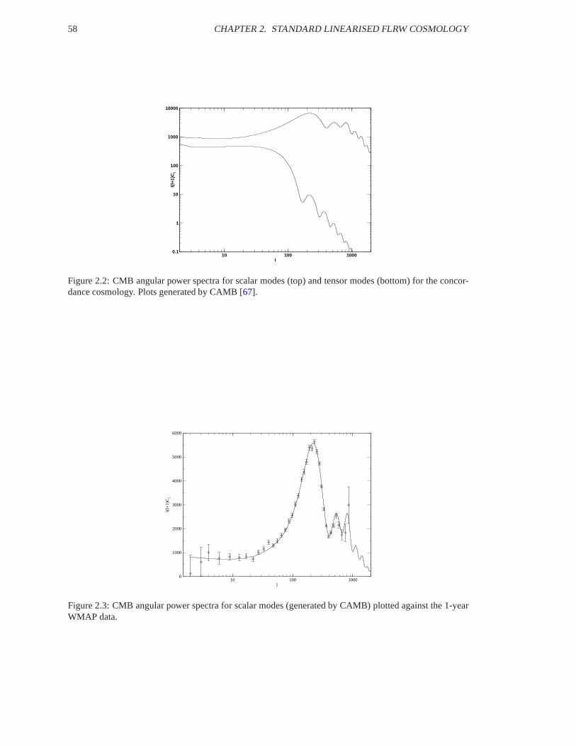
58 CHAPTER 2. STANDARD LINEARISED FLRW COSMOLOGY

10 100 1000l

0.1

1

10

100

1000

10000

l(l+

1)C

l

Figure 2.2: CMB angular power spectra for scalar modes (top)and tensor modes (bottom) for the concor-dance cosmology. Plots generated by CAMB [67].

10 100 1000l

0

1000

2000

3000

4000

5000

6000

l(l+

1)C

l

Figure 2.3: CMB angular power spectra for scalar modes (generated by CAMB) plotted against the 1-yearWMAP data.

Chapter 3

Magnetised Cosmology

3.1 The Electromagnetic Field

In this chapter we consider the additions to the standard linearised cosmology that a tangled primordialmagnetic field will introduce. After reducing more general expressions to a suitable cosmological ap-proximation we then consider in some detail the transferralof the magnetic terms into Fourier space. Weconclude with a brief review of the damping of magnetohydrodynamical modes by photon shear viscosity.

While much of the material presented in this chapter is known, the approach is entirely individual andthe equations formulated more generally than has previously been seen in the metric based approach. Tsagasand Maartens [71, 72] and Lewis [59] work within the gauge-invariant and covariant formalism,and so inprinciple present a greater generality and consider first the full non-linear equations before truncating themto some expansion order. However, Lewis does not consider the scalar perturbations and the work Tsagasand Maartens is limited to a homogeneous field. Giovannini [6] works within a metric-based approachand presents equations to a similar generality but considers only scalar perturbations. For future ease wepresent equations with the electromagnetic fields held to anarbitrary perturbation order before linearisingtheir effect; this will aid a two-parameter perturbation approach.

3.1.1 Field and Stress-Energy Tensors

In an inertial frame, the electromagnetic field tensor, or Faraday tensor, can be defined by

F ′µν = 2A[ν,µ] = Aν,µ −Aµ,ν

whereAµ = (−φ,A)

is the 4-potential andφ andA the scalar and vector electromagnetic potentials respectively. The electricfield~ǫ and magnetic field~β can be found from

~β = ∇× A, ~ǫ = −∇φ− ∂A

∂t(3.1)

where for the moment we are employing co-ordinate time. Since these are in Minkowski space we haveβi = βi andǫi = ǫi. This gives the field tensor in a matrix format as

F ′µν =

0 −ǫ1 −ǫ2 −ǫ3ǫ1 0 β3 −β2

ǫ2 −β3 0 β1

ǫ3 β2 −β1 0

. (3.2)

Extending Jedamzik, Katalinic and Olinto [69], we obtain the FLRW form of this from the locally-Minkowskitensors above by transforming from Minkowski space to a perturbed FLRW metric using (2.74, 2.76). This

59

60 CHAPTER 3. MAGNETISED COSMOLOGY

gives a field tensor

Fµν = a2

0 −ǫ1 −ǫ2 −ǫ3ǫ1 0 β3 −β2

ǫ2 −β3 0 β1

ǫ3 β2 −β1 0

+1

2a2

0 −ha1ǫa −ha2ǫa −ha3ǫaha1ǫa 0 hβ3 − ha3βa − (hβ2 − ha2βa)ha2ǫa − (hβ3 − ha3βa) 0 hβ1 − ha1βaha3ǫa hβ2 − ha2βa − (hβ1 − ha1βa) 0

,

Fµν =1

a2

0 ǫ1 ǫ2 ǫ3−ǫ1 0 β3 −β2

−ǫ2 −β3 0 β1

−ǫ3 β2 −β1 0

+1

2a2

0 −h1aǫa −h2

aǫa −h3

aǫa

h1aǫa 0 −

(

hβ3 − h3aβ

a)

hβ2 − ha2βaha2ǫa hβ3 − ha3βa 0 − (hβ1 − ha1βa)ha3ǫa − (hβ2 − ha2βa) hβ1 − ha1βa 0

.

The electric and magnetic fields observed by a comoving observer withuµ = a−1(1, 0) can then be recov-ered [68, 71, 72] by

eµ = uνFµν , bµ =

1

2εµαβFαβ (3.3)

with corresponding covariant expressions. Note that we areactually computing the electric field and mag-netic fieldh; our use of the magnetic induction in this case is habitual and the approximations we shall soonapply make the field and induction vectors equal.εµαβ =

√

−|gσρ|ǫµαβ is the Levi-Civita tensor densityfor this space andǫµαβ the totally anti-symmetric tensor density.

The co- and contra-variant forms of the electric and magnetic fields are

eFLRWµ = a

(

0, ǫi +1

2hai ǫa

)

, bFLRWµ = a

(

0, βi +12h

ai βa)

, (3.4)

eµFLRW = a−1

(

0, ǫi − 1

2hiaǫ

a

)

, bµFLRW = a−1(

0, βi − 12h

iaβ

a)

. (3.5)

We shall work with the comoving vectorsei = ǫi + (1/2)hai ǫa and bi = βi + (1/2)hai βa, and it istacitly assumed that they contain these internal structures. However, it is worth commenting that theseforms for the electric and magnetic fields are more general than those presented in [69], for example. Inprevious work, authors have employed the conformal equivalence of Minkowski and Robertson-Walkermagnetohydrodynamics [49] to map the locally-observed Minkowski fields directly ontothe Robertson-Walker fields, that iseFLRW

i = aǫi, bFLRWi = aβi. This is sufficient for fields present in the background

but not for a perturbed Robertson-Walker metric, which is nolonger conformally Minkowski. The resultsfound by [52, 53, 55] are no less valid, since the fields are assumed small and the coupling terms implicitlyto be of orderO(ε3/2). The forms presented above, however, should be employed if one wishes to considerfields of a different order or, indeed, fields in a Robertson-Walker metric perturbed to second order.

The stress-energy tensor of the magnetic fields is then given[68, 96] by

4πT µν = FµσFνσ − 1

4δµνF

σρFσρ. (3.6)

Noting, then, thatF σρFσρ = 2

(

b2 − e2)

,

3.1. THE ELECTROMAGNETIC FIELD 61

one can construct the energy density, momentum flux and momentum flux density of an electromagneticfield:

4πT 00 = F 0σF0σ − 1

4F σρFσρ = −1

2

(

e2 + b2)

, (3.7)

4πT i0 = F iσF0σ = F ijF0j = − (e× b)i (3.8)

4πT ij = F iσFjσ − 1

4δijF

σρFσρ. =1

2

(

b2 + e2)

δij − eiej − bibj . (3.9)

We have recovered the familiar energy density of an electromagnetic field, the Poynting vector, and theelectromagnetic stresses. The latter separate into the isotropic pressure

4πT ii = 4π (3p) =1

2

(

b2 + e2)

, (3.10)

which gives the expected equation of statep = (1/3)ρ, and the anisotropic stress

4πΠij =

1

3

(

b2 + e2)

δij − eiej − bibj. (3.11)

3.1.2 Maxwell Equations and Stress-Energy Conservation

The Einstein equations are not the only equations governingthe evolution of the electromagnetic field. Onealso has the Maxwell equations, Ohm’s law and stress-energyconservation.

The electromagnetic 4-current is taken to be

jµ = a−1 (, j) (3.12)

where is the comoving charge density andj the comoving charge current density. This is a 4-current asobserved in a frame comoving with universal expansion. In a locally-Minkowski frame, one would expectto observe a currentjMink = j − v.1

The Maxwell equations are then

Fµν;ν = jµ, F[λµ;σ] = 0. (3.13)

The skew-symmetry of the electromagnetic field tensor implies charge conservation

jµ;µ = 0. (3.14)

The relativistic equivalent to the familiar Ohm’s law arises when one projects the (invariant) 4-current intothe observer’s 3-space and sets this observed current proportional to the electric field viewed in this frame[68, 71, 103] – that is

Hµνjν = (gµν + uµuν) j

ν = σFµνuν ⇒ jµ + uµuνj

ν = σFµνuν . (3.15)

σ is the electrical conductivity.One may rapidly demonstrate that the Maxwell equations in a synchronous FLRW metric perturbed to

first order, with electromagnetic fields held to arbitrary order, are

F 0ν;ν=j0 : ∇ · e +

1

2(e · ∇)h = a,

F iν;ν=ji : ∇× b−

(

e + 2a

ae

)

− 1

2he − 1

2(b ×∇)h = aj, (3.16)

F[0ij]=0 : b + 2a

ab + ∇× e = 0,

F[ijk]=0 : ∇ · b = 0.

1This takes the opposite sign to that one might naıvely expect since our velocity is defined with reference to the comovingexpansionrather than with reference to a Minkowski observer.

62 CHAPTER 3. MAGNETISED COSMOLOGY

The requirement of charge continuity implies that

˙ + 3a

a+ ∇ · j +

1

2h+

1

2(j · ∇)h = 0. (3.17)

Interpreting this in the absence of metric perturbations, we see that there is an effective “sink” of charge (asviewed by a comoving observer) caused by the universal expansion – charge decays asa−3.

The spatial part of Ohm’s law gives

j− v = σ (e + v × b) (3.18)

which is the familiar Ohm’s law from electrodynamics. The temporal component yields, toO(ǫ), v · j =σv · e which is merely the scalar product of the standard Ohm’s law with the observer’s velocity.

Generalising the results of (for example) Jedamziket. al. [69] to the case of finite conductivity and aperturbed universe, the contributions of electromagneticfields to stress-energy conservation are

− 4πT ν0;ν = e · e + b · b + 2a

a

(

e2 + b2)

+ ∇ · (e× b) +1

2

(

e2 + b2)

h

+1

2((e× b) · ∇)h− 1

2hij(

eiej + bib

j)

= −ae · j − 1

2

(

hb2 +

(

hij + 2a

ahij

)

(

eiej + bib

j)

)

, (3.19)

4πT νi;ν = ∂η (e× b)i +1

2∂i(

b2)

+1

2∂i(

e2)

+

(

4a

a+

1

2h

)

(e× b)i

−1

2ei ((e · ∇)h) − 1

2bi ((b · ∇)h) +

a

ahji (e× b)j

+1

2

(

ejek + bjb

k)

∂ihjk − ∂j

(

eiej + bib

j)

= −a (j× b)i − aei +1

2(b× (b×∇))i h− 1

2bi (b · ∇)h

+a

ahji (e × b)j +

1

2

(

ejek + bjb

k)

∂ihjk. (3.20)

The first of these is the contribution an electromagnetic field will make to the conducting fluid’s masscontinuity; the field creates fluctuations in the fluid’s current which then impacts on the matter conservation.The second of these is the contribution the field makes to the Euler equation (momentum conservation).Comparing with the form for non-relativistic magnetohydrodynamics (e.g. [116]) we can pick out theimportant contributions to the Euler equation

l = a (j × b + e) (3.21)

which is the standard Lorentz force. All other terms in the Euler contribution are couplings to the metricperturbations, representing the scattering of the fields from the underlying geometry. This coupling isreadily apparent in covariant approaches to the problem (see for example [68, 71, 72, 87]) in the full non-linear equations, where the fields couple directly to the Weyl tensor.

3.1.3 The Electromagnetic Field: Robertson-Walker and Bianchi Cosmologies

The Robertson-Walker cosmology is a cosmology homogeneousand isotropic about every event, at least tozeroth order, which forbids the addition in the background of a directional field. The electromagnetic fieldgenerally produces both an energy flux and a full anisotropicshear, neither of which are compatible with aRobertson-Walker metric.

To maintain the standard cosmology, it is necessary to ensure that the energy flux and anisotropic shearvanish at zeroth order in the perturbation parameterε. To retain the FLRW form we thus set the electromag-netic fields to be “half-order”; that is, that we should setO(e, b) ≈ O(

√ε). While this has the benefit of

removing electromagnetic shear from the bulk cosmology, itis restrictive for two main reasons: firstly thata linearisation of the magnetic field employing the same parameter will push the perturbed fields to one-and-a-half order and our field will be correspondingly bland, and secondly that the scattering of the fields

3.2. BARYONIC MATTER: COSMOLOGICAL MAGNETOHYDRODYNAMICS 63

from gravity is also pushed to one-and-a-half order. This neglects many of the more interesting effects of amagnetic field, such as the direct sourcing of tensor perturbations, and removes almost the entire structureof MHD. (See [52] for some further discussion on this matter.) It does, however, mean that the comovingfields in the Robertson-Walker metric can now be identified with the Minkowski fields.

However restrictive in linear perturbation theory our approach may be, it allows a great freedom in theexact form of the fields that one may add. The modern approach in CMB physics is to employ a half-ordertangled stochastic magnetic field, (with or without a homogeneous component) under the assumption thatthe initial spectrum is Gaussian and the tangled component has one or more length scales (e.g. [49, 51, 52,53, 55, 61]). The fields are usually assumed to be tangled on cluster scales – implying no directionalityon supercluster scales – and the observed strength on such scales can be used to fix the amplitude of themagnetic power spectrum.

The net effect of these assumptions, along with taking the limit of infinite conductivity, is merely to addto the standard Euler equation a Lorentz force. The magneticfield influences not only the temperature mapsfor the CMB but also the polarisation – indeed, it is likely that the effect on the temperature-temperaturepower spectrum will be sub-dominant across most of the realistically observable range, and the effects ofa magnetic field might be observable primarily by its imprinton the polarisation (e.g. [85, 54, 57, 55]) orperhaps its non-Gaussianity [53, 163, 164].

An alternative approach, while still remaining within the constraints of a Robertson-Walker cosmology,would be to employ a two-parameter linearisation approach,with a magnetic field too small to affect thebulk cosmology linearised by a free parameterεB. One would neglect terms of orderO(ε2, ε2B) but re-tain those of orderO(εεB) A brief study of two-parameter perturbation theory (in the context of but notrestricted to rotating, relativistic stars) is presented by Bruni et. al. [165] and the referenced works therein.

Were one to drop the condition of isotropy and introduce a mildly isotropic Bianchi cosmology ratherthan the maximally symmetric FLRW, then one could instead employ a magnetic field that gives the universea preferred direction. It would also be possible to include the shear viscosity of the baryons (and possiblyalso of the CDM) at zeroth order which could potentially model a realistic fluid more than the perfect fluidapproximations. Indeed, the limits that Barrow, Ferreira and Silk place on the strength of a bulk field [62],based on the 4-year COBE results, are derived by limiting theanisotropy introduced by a Bianchi (typeVII) model and attributing it entirely to a magnetic field. The idea of imposing a preferred direction on theuniverse through an ordered magnetic field, while certainlynot original (research in magnetised anisotropiccosmologies goes back to at least the late 60s; see [38, 39, 40] and references therein) could correspond toTegmarket. al.’s speculative explanation [159] for the low power observed in the quadrupole by WMAP[78, 166] resulting from a preferred direction. It is also interesting to note that Tsagas and Maartens havedemonstrated [87] that, for a relatively weak field, the Robertson-Walker approximation is equivalent atfirst order to a Bianchi I approach.

3.2 Baryonic Matter: Cosmological Magnetohydrodynamics

3.2.1 Real Space

We now consider a magnetised baryon fluid. In the presence of amagnetic field, the mass continuity andEuler equations, retaining for generality the pressure terms and including again the collisional termCib→γ

transferring momentum between the baryons and the photons,become

ρ+ ∇. ((ρ+ p)v) +

(

3a

a+

1

2h

)

(ρ+ p) − 1

4πae · j

− 1

8π

(

hb2 + hij(

eiej + bib

j)

)

= 0,

∂

∂η

(

(ρ+ p) vi)

+ ∂ip+ 4a

a(ρ+ p) vi − a

4π(j× b)i − a

4πei

+1

8π(b× (b×∇))i h− 1

8πbi (b · ∇)h+

1

4π

a

a(e× b)j hij

+1

8π

(

ejek + bjb

k)

∂ihjk + Cib→γ = 0.

These are supplemented by the Maxwell equations (3.16), charge continuity (3.17) and Ohm’s law (3.18).

64 CHAPTER 3. MAGNETISED COSMOLOGY

Clearly these equations are not in an ideal form either for further analytical study or for numericalimplementation. Instead, we shall follow the lead of [50, 35, 69, 70] in rescaling the magnetic fields toremove the Hubble terms in the Maxwell equations.

One may rapidly demonstrate that the Maxwell equations reduce (in the absence of metric perturbations)to the form of classical electrodynamics if one employs the scalings

E,B, a,J, σa =

a2e, a2b, a3, a3j, a−1σ

(3.22)

with no scaling for the comoving co-ordinates (and hence none for ∂i and∇), the baryon velocity or themetric perturbation. These are generally physically motivated; the electric and magnetic fields scale witha2 because their energy density must be that of radiation and decay asa4. The charge and current densities,associated with matter, are scaled bya3. The conductivity has dimensions of length and so scales with a.

With these new variables, the electrodynamical equations reduce to

∇ ·E = a − 12 (E · ∇)h

∇× B− E = J + 12 hE + 1

2 (B×∇)h

B + ∇× E = 0∇ ·B = 0

˙a + ∇ · J = − 12

(

ah− (J · ∇)h)

J − av = σa (E + v × B) .

(3.23)

In the equations of cosmological MHD presented above, we seewe should then apply the scaling

ρba, pba = a4 ρb, pb (3.24)

to the mass density and pressure respectively. This scalingis not performed to erase Hubble terms butinstead to ensure that each term is scaled by the same factor;our scalings were employed to reduce the un-perturbed cosmological Maxwell equations to the Minkowskiform, rather than remove the time-dependenceof each variable. Consistency of scaling then requires thatthe matter density and pressure are scaled as themagnetic density and pressure are – asa4 rather than asa3 as one would naıvely expect. (Subramanian andBarrow [70] present a more formal and detailed analysis of the conformal relation between magnetohydro-dynamics in an unperturbed Robertson-Walker metric and in aMinkowski metric.) Note also that

pba = wa (ρba) ρba ⇒ pb = wa (ρba) ρb

which implies thatwa (ρba) = w (ρb) . (3.25)

We also have

c2s =∂p

∂ρ= c2sa. (3.26)

Employing these substitutions, the MHD equations quickly become

ρba + ∇ · ((ρba (1 + w))v) +1

2(ρba (1 + w)) h

=a

aρba (1 − 3w) +

1

4πE · J +

1

8π

(

hB2 + hij(

Ei(x)Ej(x) +Bi(x)Bj(x))

)

, (3.27)

vi +

(

w

1 + w+ρbaρba

)

vi +c 2s

ρba (1 + w)∂iρba +

1

1 + wCib→γ

=1

4π (1 + w) ρba(J × B + aE)

i+

1

8π (1 + w) ρba

(

Bi(x) (B · ∇)h− (B× (B×∇))ih

−2a

a(E × B)

jhij +

(

Ej(k)Ek(x) +Bj(x)Bk(x))

∂ihjk

)

. (3.28)

3.2. BARYONIC MATTER: COSMOLOGICAL MAGNETOHYDRODYNAMICS 65

Linearisation

We expand around the FLRW background by setting

ρba = ρba (1 + εδ) , O(vi) ≈ O(ε), B,E,J, a →√ε B,E,J, a .

The (dimensionless) perturbation to the densityδ is naturally unscaled. The comoving electric and magneticfields can then be identified with their Minkowski equivalents,

ei = ǫi, bi = βi

and the contra- and co-variant components are equal. Neglecting all powers ofε above unity and separatinginto background and perturbation leads to the Maxwell equations

∇ · E = a,

∇× B − E = J,

B + ∇× E = 0,∇ ·B = 0,

˙a + ∇ · J = 0,J = σaE,

(3.29)

supplementing the magnetohydrodynamical equations

ρba =a

aρba (1 − 3w) , ∇ρba = 0

in the background and

δ + (1 + w)∇ · v +1

2(1 + w) h =

1

4πρbaE · J,

vi +

(

w

1 + w+a

a(1 − 3w)

)

vi

+c 2s

(1 + w)∂iδ +

1

1 + wCib→γ =

1

4πρba (1 + w)(J × B + aE)i .

at first order.For baryonic matter we again setw = c2s = 0 except where they multiply a spatial derivative giving

ρba =a

aρba → ρba ∝ a; ∇ρba = 0 (3.30)

and

δb + (1 + w)∇ · vb +1

2h =

1

4πρbaE · J, (3.31)

vi +a

avi + c2s∂

iδb + Cib→γ =1

4πρba(J × B + aE)

i ≡ 1

ρbaLi. (3.32)

One can now clearly see that the only difference in the Euler equation obeyed by the baryons with a magneticfield of this type, compared with the standard cosmological picture (2.155), is the existence of the LorentzforceL. The greater structure of the interactions between the magnetic fields, the geometry, and the per-turbations is at a higher-order. This complex structure gives rise to, for example, direct coupling betweenthe magnetic fields and the Weyl tensor ([71]) and magnetic fields automatically sourced by second-ordervorticity ([31, 32]). The vast bulk of cosmological MHD remains unexplored.

Early-Universe Approximations

It is usual to assume that the conductivityσa is extremely high until after recombination (see for example [4]or the appendix of [17]); this loose statement may be quantified by considering thedimensionless magnetic

66 CHAPTER 3. MAGNETISED COSMOLOGY

Reynolds number

RB = 4πµ0σ|∇ × (v × B)|

|∇2B| ≈ 4πµ0σvL (3.33)

whereL is the typical length-scale of the system. To a good approximation, the universe possesses alow Reynold’s number for much of its evolution. Using Ohm’s law, assuming a vanishing conductivitywhile retaining a finite current density then removes the electric fields. This is sometimes dubbed themagnetohydrodynamical limit. It is also standard in MHD (see [116]) to take the displacement current asnegligible for non-relativistic scenarios; the situationhere is highly non-relativistic, and so we shall alsoemploy this approximation.

The equations now become

J = ∇× B, B = 0, a = 0, ∇ ·B = 0, ρba =a

aρba, (3.34)

and so

δb + (1 + w)∇ · vb +1

2h = 0, (3.35)

vib +a

avib + c2s∂

iδb + Cib→γ = =1

ρbaLi.

The total stress-energy tensor for these two fluids is

T0

0 = ρb, Ti

0 = Ti

j = 0, (3.36)

δT 00 = ρbδb +

1

8πa4B2(x), δT i0 = −ρbvib, (3.37)

δT ii =1

8πa4Bm(x)Bm(x), δΠi

j =1

4πa4

(

1

3Bm(x)Bm(x)δij −Bi(x)Bj(x)

)

. (3.38)

The scaled magnetic fieldB(x) is independent of time and so, if one postulates a strength for the mag-netic field in the present epoch and normalises the scale factor so thata(η0) = 1, the present value can beemployed throughout. This assumes that the conductivity ofthe universe remains negligible after recom-bination; while the conductivity is likely to remain extraordinarily high, this is not going to be an entirelyvalid assumption. Moreover, this assumption neglects any non-linear effects on the magnetic field. In effectwe have neglected the action of both gravity and, indeed, magnetohydrodynamics, and any conclusionsbased on the above model after recombination should be treated with caution.

3.2.2 Fourier Space

Even with our simplifying assumptions, the cosmological MHD equations form a complicated set of equa-tions; however, despite the non-linear nature of the Lorentz force and the stress-energy tensor of the mag-netic fields, we shall find the system is rendered somewhat more tractable in Fourier space.

Consider first the scaled Maxwell equations and conservation of charge, which are linear and so willnot be convolved. In Fourier space we see that these are

B(k) = 0, k · B(k) = 0 (3.39)

where we have neglected the trivial equations. The magneticstress-energy tensor in real space has theisotropic and anisotropic stresses

4πa4T ii = 4πτ ii =1

2Bm(x)Bm(x),

4πa4Πij =

1

3Bm(x)Bm(x)δij −Bi(x)Bj(x),

3.2. BARYONIC MATTER: COSMOLOGICAL MAGNETOHYDRODYNAMICS 67

with a vanishing Poynting vector and the energy density equal to a third of the isotropic stress. We employτµν to denote the scaled stress-energy tensor. The isotropic pressure is transferred to Fourier space by

4πτ ii (k) =1

2

∫

Bm(x)Bm(x)eik.xd3x

=1

2

∫∫

Bm(k′)Bm(x)ei(k−k′).xd3xd3k′

2π3

=1

2

∫

Bm(k′)Bm(k − k′)d3k′

2π3

which is the expected convolution. Note that the reality of the fields in co-ordinate space requiresB(k) =−B∗(k). For the anisotropic stresses we have

4πa4Πij(k) =

∫

1

3Bm(k′)Bm(k − k

′)δij −Bi(k′)Bj(k − k′)

d3k′

2π3. (3.40)

The scalar, vector and tensor parts are derived from this by applying combinations ofP ij (k),Qij(k),PV ijk (k)

andPTijab (k) as in equations (2.18). We find

4πτS(k) = 4πQji (k)

(

1

3τaa (k)δij + Πi

j

)

=3

2kj ki

(

4πΠij(k)

)

=1

2

∫

Bm(k′)Bm(k − k′) − 3(

k ·B(k′))(

k · B(k − k′)) d3k′

2π3(3.41)

for the anisotropic pressure. For the magnetic vorticity weemploy the symmetrised vector projection whichgives us

4πτVa (k) = 4πPV ija (k)

(

1

3τaa (k)δij + a4Πi

j

)

(3.42)

= k(iPj)a (k)

(

4πa4Πij(k)

)

=

∫

(

k · B(k′))(

k ·B(k − k′))

ka −1

2

(

k · B(k′))

Ba(k − k′)

−1

2

(

k · B(k − k′))

Ba(k′)

d3k′

2π3, (3.43)

and the symmetrised tensor projection likewise gives us

4πτaTb = 4πa4PajTbi Πij

=1

2

∫

Bm(k′)Bm(k − k′)(

δab − kakb

)

− 2B(a(k′)Bb)(k − k′)

−(

k ·B(k′))(

k · B(k − k′))(

δab + kakb

)

+2(

k · B(k′))

k(aBb)(k − k′) + 2(

k ·B(k − k′))

k(aBb)(k′)

d3k′

2π3(3.44)

We shall study this stress-energy tensor in much greater detail in the next chapter and content ourselveshere with commenting that this highly-nonlinear form will naturally introduce to the system a significantmeasure of non-Gaussianity, even for a magnetic field which is itself Gaussian in nature. It should also becommented that while our simplified system will retain the Gaussianity of these fields the preservation ofGaussianity of a magnetic field in general is not necessarilyto be expected.

Turning now to the Lorentz forces, in co-ordinate space we had that

4πL(x) = (∇× B(x)) × B(x)

68 CHAPTER 3. MAGNETISED COSMOLOGY

for the infinitely conductive universe. Following the same process to push this into Fourier space, we have

4πL(k) =

∫∫

(∇× B(k′)) × B(x)ei(k−k′).xd3xd3k′

2π3

= −i∫∫∫

(k′ × B(k′)) × B(k′′)ei(k−k′−k′′).xd3xd3k′

2π3

d3k′′

2π3

= −i∫∫

(k′ × B(k′)) × B(k′′)δ(k − k′ − k′′)d3k′d3k′′

2π3(3.45)

where we have used(2π)3δ(k − k′) =∫

ei(k−k′).xd3x. Employing

((A × B) × C) = C(A · B) − B(A · C) (3.46)

we can write

4πL(k) = −i∫

B(k′)(

k′ · B(k − k′)) d3k′

2π3(3.47)

where we have also used Maxwell’s third equation,k · B(k) = 0. If we now use the freedom we have inour integration wavemode to writek′ → k − k′ thend3k′ → −d3k′ and the Lorentz force becomes thesimple

4πLj(k) = ik

∫

Bj(k − k′)(

k · B(k′)) d3k′

2π3(3.48)

where again we have used Maxwell’s third equation. We can nowsplit this into a scalar part,

4πLS = −ik · L(x) = k

∫

(

k ·B(k′))(

k · B(k − k′)) d3k′

2π3

which, comparing with the scalar pressures is

LS =2k

3

(

τ ii − τS)

=2k

3P ij (k)τ ji (k), (3.49)

and an (unsymmetrised) vector part

4πLVi (k) = P ai (k)La(k) = ik

∫

(

k · B(k′))(

Bi(k − k′) −(

k · B(k − k′))

ki

) d3k′

2π3

which is readily seen to beLVi (k) = ikτVi (k). (3.50)

That is, the scalar contribution to the Lorentz force is directly proportional to the difference of the iso- andaniso-tropic pressures, while the vortical contribution to the Lorentz force is directly proportional to themagnetic vorticity itself, when seen in Fourier space.

Considering the full baryon fluid, then, aligning the co-ordinate axes along the Fourier mode and em-ploying the vector and tensor bases defined in§2.3.2results in the stress-energy tensor

T0

0 = −ρb, T0

i = Ti

j = Πij = 0 (3.51)

in the background and

δT 00 = −ρbδb −

1

a4τ ii , δT i(0)S = −ρbvbS , δT i(0)V = −ρbvibV ,

δT ii =1

a4τ ii , δTS =

1

a4τS , δT Vi =

1

a4τVi , (3.52)

δT T+ =1

8πa4

∫

B2(k′)B2(k − k′) −B1(k

′)B1(k − k′) d3k′

(2π)3 ,

δT T× =−1

8πa4

∫

B1(k′)B2(k − k

′) +B1(k − k′)B2(k

′) d3k′

(2π)3 .

3.3. DAMPING OF COSMOLOGICAL MAGNETIC FIELDS 69

The equation of mass continuity becomes

δb + (1 + w) kvS +1

2h = 0. (3.53)

The scalar component of the Euler equation is

vbS +a

avbS − kc2sδ + cSb→γ =

2

3ρbak(

τ ii − τS)

(3.54)

and the vector component is

vVi +a

avVi + (V )cb→γ

i =i

ρbakτVi . (3.55)

This then completes the system of equations that one would need to include in a Boltzmann integrator –CMBFast [76] would be ideal due to its use of synchronous gauge – to include a primordial magnetic fieldalong with a standard cosmology.

3.3 Damping of Cosmological Magnetic Fields

In this section we shall review the pertinent results of [35, 52, 55, 69, 70] governing the scales at whichmagnetohydrodynamical modes in the universe are damped by viscous processes. This scale,kD, it shouldbe emphasised, is distinct from an inherent magnetic damping scale arising from some particular magne-togenesis model, being viscous in origin and arising from the shear drag imposed on the baryons by thephoton fluid. The primordial damping scale is likely to be very small and constant, while the viscous damp-ing scale will be somewhat larger and time-dependent. The effective damping scale of the magnetic fieldwill then be

kc(η) = min(

kprimc , kD(η)

)

. (3.56)

At some epoch, therefore, the effective magnetic damping scale will become time-dependent.Mode damping is a small-scale effect of the photon (or neutrino) viscous drag on the coupled photon-

baryon fluid; to analyse it we return to real space and, for ease of mathematics, linearise the magnetic fieldaround an ordered background with

B = B0 + B1, B0 = 0, B0 = B0z.

We employ a shear viscosity to model the photon viscosity (see appendixB), impose infinite conductivityand, since we are working on scales much less than the Hubble scale, neglecta/a. We have the system ofequations

δ + ∇ · v = 0,ρbaρba

≈ 0, (3.57)

v + c2s∇δ =1

4π(ρba + pba)(B0 × (∇× B1)) + ξa

(

∇2v +1

3∇ (∇ · v)

)

, (3.58)

B1 = ∇× (v × B0) . (3.59)

We may then derive a wave equation forv,

v − c2s∇ (∇.v) = vA × (∇× (∇× (v × vA))) + ξa

(

∇2v +1

3∇ (∇ · v)

)

. (3.60)

We have defined the Alfven velocity

vA =B0

√

4π(ρba + pba). (3.61)

70 CHAPTER 3. MAGNETISED COSMOLOGY

In Fourier space this becomes

v +(

c2s + v2A

)

(k · v)k

= (k · vA) (v(k · vA) − k(v · vA) − vA(k · v)) − ξa

(

k2v +1

3k(k · v)

)

. (3.62)

We align the magnetic field with thez-axis and definek · vA = kvA cos θ andv · vA = vz. Then wecan consider various perturbation modes:

• Incompressible waves: Alfven Waves

If we take∇ · v = 0 ⇒ k · v = 0 then by the continuity equation we are considering perturbationsthat do not support density perturbations. In the wave equation, we then see that

v +3ξa4ρba

k2v + k2v2A cos2 θv = 0. (3.63)

These waves will then oscillate whenkvA cos θ ≫ 3ξak2/4ρba, and will overdamp whenkvA cos θ ≪

3ξak2/4ρba. For photons, we have the shear viscosity [70]

ξa =8

15

π2

30Θ4lγ (3.64)

whereΘ is the temperature andlγ = (neσT )−1 the mean photon diffusion length. From here it canbe shown that the ratio of the friction term to the natural frequency is approximately

D

ω0≈ 530

k

a(η)

lγ(η)

B−9(3.65)

whereB−9 is the background field in units of nano-Gauss. Many modes will thus be overdamped. Ofthe two solutions of a heavily damped oscillator we expect one, with a large initial velocity, to damprapidly, and another with a small initial velocity to effectively freeze. It is this second mode that willsurvive Silk damping.

• Magnetosonic Waves

Consider now the compressible waves; definingvk = k.v and taking inner products of the waveequation with firstk and thenz we can find the two equations

vk +(

c2s + v2A

)

k2vk − k2v2A cos2 θvz +

ξaρba

k2a = 0, (3.66)

vz + c2sk2 cos θvk +

3ξa4ρba

k2vz +ξa

4ρbak2 cos θvk. (3.67)

Taking a mode parallel to the magnetic field (k ‖ vA) gives

vk +ξaρba

k2vk + c2sk2vk = 0 (3.68)

which is a standard, Silk-damped, sound wave. If we considera wavevector perpendicular to themagnetic field,k ⊥ vA, we instead find

vk +ξaρba

k2vk −(

c2s + v2A

)

k2vk = 0 (3.69)

which is a damped fast magnetosonic wave. This damps in the same way as a standard sound wave.

Finally if we consider a wavevector tilted with respect to the field,k.vA = kvA cos θ, we have a slowmagnetosonic wave. Subramanian and Barrow showed that thisbehaves approximately as the Alfvenwaves, though the analysis is slightly more involved. A different approach with the same conclusionswas presented in [69].

3.3. DAMPING OF COSMOLOGICAL MAGNETIC FIELDS 71

To briefly summarise, then, we have seen that, during the tightly-coupled epoch, fast magnetosonicwaves sourced by a magnetic field will damp as sound waves, while one mode apiece of the slow magne-tosonic waves and Alfven waves will become strongly overdamped and freeze, thus surviving Silk damping.

Free-streaming occurs when the mean free path of the photonlγ = (neσT )−1 grows larger than thewavelength of a given mode. At decoupling this is around3Mpc, and after recombination all of the modeswill freely stream. Accurate evaluation of modes in the free-streaming regime requires a full treatmentof the photon and baryon fluids; however, Subramanian and Barrow provide an approximate treatment,considering the Euler equation

v +a

av + (v · ∇)v = − 1

ρb∇pb +

1

ρbj × b− 1

a∇φ− 4

3

ργρbaneσTv (3.70)

whereφ is the gravitational potential from Poisson’s equation. Wethen have two chief regimes, one inwhich the magnetic pressure dominates over the baryon pressure, and the opposite. When the baryonpressure dominates, one may derive an evolution equation for the velocity

v +

(

a

a+

4ργ3ρb

aneσT

)

v +4ργ3ρb

k2v2Av = 0. (3.71)

The Hubble damping will be much smaller than the viscous damping and so the ratio between the dampingand natural frequency is

D

ω0=

√

4ργ3ρb

aneσTkvA

≈ (3 × 103)

√

ργρb

((k/a)lγ(η)B−9)−1 (3.72)

which, given that we are free-streaming and(k/a)lγ ≈ 1, and that we are considering particularly weakfields, is strongly overdamped.

Employing a “terminal-velocity” approximation for the low-amplitude mode which is effectively frozen– that is, neglecting the acceleration – one can find rough solutions to the equations. In this regime thesolution is rapidly

v(η) = v(ηf )e−

„

R

η

ηf

ω20

Ddη

«

= v(ηf )e−v2A cos2 θ

R

k2a2lγdt = v(ηf )e− k2

k2D . (3.73)

where we have swapped the integral to co-ordinate time for neatness. This allows us to identify the dampingscale

k−2D = v2

A cos2 θ

∫

lγ(t)

a2(t)dt. (3.74)

This is at a minimum at recombination, and evaluated at recombination and comparing with the Silk scalewe have

k−1D ≈

√

3

5vALS . (3.75)

The analysis in the case of a stronger field is more complicated and unlikely to be necessary given therelative weakness of the primordial cosmological field.

In general we will take the damping scale to be approximately

k−1D ≈

√

3

5vAlγ (3.76)

wherelγ is the photon diffusion length. The Alfven modes that survived Silk damping will be convertedinto fast and slow magnetosonic waves. The damping scales are similar to that above for fast waves, whilefor slow waves the baryon speed of sound dominates over the Alfven velocity. The time-dependence of theviscous damping scale arises from the photon diffusion length; for the more complicated case of a tangledfield configuration, addressed in chapter5, the Alfven velocity is also time-dependent.

For further discussion on damping scales see appendix A of [23].

72 CHAPTER 3. MAGNETISED COSMOLOGY

3.4 Conclusions

We have presented, in a synchronous gauge, the sources and Lorentz forces arising from a magnetic field ofarbitrary size and type. We have then reduced the resulting system to a realistically tractable approximationreminiscent of standard MHD and found that the only difference between a magnetised and a standardcosmology at linear order is the existence of a Lorentz force. This Lorentz force is proportional to thestresses when viewed in Fourier space. This system is in an ideal form to transfer to some Boltzmanncode; our motivation is to construct a formalism suitable for CMBFast, although we could also employCMBEasy [143]. We also briefly considered the damping scales relevent to the problem, working in analtered formalism with a large-scale homogeneous field and asmall perturbation to address issues that areotherwise only present in second-order magnetised theories. We derived the form of the viscous dampingscale that will determine both the scale on which Alfven andslow magnetosonic perturbations are cut-off,and also the scale on which the magnetic field will ultimatelydamp.

Chapter 4

Statistics of Cosmic Magnetic Sources

4.1 Tangled Magnetic Fields

In this chapter we consider in detail the nature and statistics of the magnetic sources through a combinationof simulated realisations and analytical study. Both have advantages and disadvantages; the simulated fieldscan be vastly more general but are limited in dynamic range and computational power, while the analyticfields are heavily restricted by mathematical limitations.In line with the modern treatment, we do notassume that the magnetic field is a large-scale, ordered fieldwith a small arbitrary perturbation, but insteadconsider entirely inhomogeneous fields tangled on some length scale (see for example Macket. al. [55]).For simplicity (and to compare with the previous literature), we assume that the magnetic fields are randomvariables obeying a Gaussian probability distribution function; however, our realisations may be formulatedmore generally than this. It should however surprise no-onethat a non-Gaussian magnetic field generatesa non-Gaussian stress-energy, and so the Gaussian case is likely to be the most intuitively informative.Analytically we are currently restricted to Gaussian fields. From equation (3.16), b ∝ a−2; we will bemodelling the time-independent scaled fieldB. The only time-dependence then arises from the dampingscale. Since this will be associated with the grid-size of the realisations this is not here an issue, though itmay need to be addressed when we come to wrap our statistics onto the CMB – for some configurationsthis will lead to time-dependent stresses, thus introducing decoherence into the sourced perturbations.

Magnetic fields, being a non-linear source with a full anisotropic stress, naturally provide sources forscalar, vector and tensor perturbations. For scalar perturbations one does not expect a significant effecton large scales. However, the contribution to the temperature auto-correlation on the microwave sky canbegin to dominate at anl of 1000 − 3000 depending on spectral index (see§§5.4.1,5.4.2or [53, 59, 61]).This effect comes both from the impact of the magnetic energyand anisotropic pressure directly onto thespacetime geometry and from the Lorentz forces imparted onto the coupled proton-electron fluid. Onealso expects a significant impact on the vector perturbations as compared to the standard picture since themagnetic fields will both directly generate vector perturbations in the spacetime and contribute vorticalLorentz forces. Prior to neutrino decoupling a primordial magnetic field acts as a source for gravitationalwaves; following neutrino decoupling there will also be a contribution from the neutrinos, which Lewis hasshown serves to cancel much of the magnetic stress [59]. Since the Lorentz forces and the stress-energytensor are both quadratic in the magnetic field, we also expect a level of non-Gaussianity to be imprintedonto the fluid and perturbations, even for a magnetic field that is itself Gaussian.

The features of the magnetic field – the Lorentz forces and thedirect sourcing of geometric fluctuations– are all contained within the stress-energy tensor. We can then consider the statistics of the stress-energytensor alone and be hopeful of characterising the majority of the non-Gaussian effects that might impact onthe CMB. The non-Gaussianity predicted from our analysis and our simulations can be projected onto theCMB sky by folding them with the transfer functions generated by the modified CAMB code [59, 67] or amodification of CMBFast [51, 61, 76]. The great benefit of our formalism derived in the previous chapteris the ease with which we may implement it into CMBFast. Care would have to be taken, however, withthe initial conditions – see Lewis [59] and Giovannini [60]. In principle, theB-mode polarisation will givethe purest magnetic signal, being sourced purely by vector and tensor perturbations; however, care wouldhave to be taken to disentangle these from anyB-modes caused by the gravitational lensing of the dominant

73

74 CHAPTER 4. STATISTICS OF COSMIC MAGNETIC SOURCES

E-mode and from other early-universe sources of gravitational wave.1 Nonetheless, even on theB-modethe contaminants will be myriad. The inherently non-Gaussian nature of the sources, both gravitational andthe Lorentz forces, offers an alternative route to characterising the nature of a primordial magnetic field.

We shall concentrate our study of the statistics on the space-space part of the magnetic stress-energytensor, the stresses, since the magnetic energy density is proportional to the isotropic pressure, and inour cosmological setting the Poynting vector vanishes. TheLorentz forces are directly proportional tocomponents of the stress-energy; loosely speaking, their properties can be found by applying prefactors ofthe wavemodes to the stress-energy results.

The (scaled) stress-energy tensor can be written

τab(k) =1

2γabτ

ii (k) − τab(k). (4.1)

where

τab(k) =

∫

Ba(q)Bb(k − q)d3q.

This chapter of the thesis is derived from work by myself and Robert Crittenden [163].

4.1.1 Underlying Statistics of the Fields

We begin by specifying the underlying statistics of the tangled magnetic fields. In Fourier space, Maxwell’ssecond law implies that

〈Ba(k)B∗b (k

′)〉 =

(

P(k)Pab(k) +i

2H(k)ǫabck

c

)

δ(k − k′) (4.2)

whereP(k) is the magnetic field power spectrum,Pab is the operator projecting vectors and tensors onto aplane orthogonal toka andkb,

Pab(k) = γab − kakb, (4.3)

andH(k) is the power spectrum of the anti-symmetric helical term (see for example [56, 167, 168].) Herewe have assumed the fields are statistically isotropic and homogeneous. If the magnetic fields are Gaus-sianly distributed, then all their statistics are determined by their power spectrum. In the interests of sim-plicity we henceforth assume that the helical component of the field vanishes; however we should note thathelicity may well be a generic feature of magnetic fields generated in the very early universe (e.g. the non-conservation of helicity during the lepton stage of the universe [169] and from the magnetic-axion coupling[170]).

The power spectrum is often taken to be a simple power law,

P(k) = Akn. (4.4)

To avoid divergences, these power law spectra are generallyassumed to have some small scale cutoff usuallyassociated with the photon viscosity damping scale; see§3.3and [49, 55, 69]. Durrer and Caprini [23, 171]demonstrate that, for a causally-generated magnetic field,the spectral index must ben ≥ 2; it must also inany event ben ≥ −3 to avoid over-production of long-range coherent fields. They also demonstrate thatnucleosynthesis limits on the gravitational waves produced by the magnetic fields place extremely strongbounds on magnetic fields, to the level of10−39G for inflation-produced fields withn = 0, although this hasbeen contested (see§5.2.2). For spectra that might realistically imprint on the microwave background wemust consider spectra withn < −2, which are much less tightly constrained. For purposes of comparisonwe shall usually take eithern = 0 for a flat spectrum – where “flat” refers to the spectrum of primordialmagnetic fields themselves – in which each mode contributes equally, orn = −2.5 for a spectrum nearingthe “realistically observable”n ≈ −3, which we shall refer to as “steep”. Such fields can be produced byinflation (for example, [21, 172]).

1Magnetic fields will also cause Faraday rotation fromE modes intoB modes [45, 46, 41, 85]; support for scalar modes in auniform magnetic field was added to CMBFast by [46] and also to CMBFast for tangled fields by [41], both in the case of smallrotations.

4.1. TANGLED MAGNETIC FIELDS 75

It is worth emphasising that, while we generally restrict ourselves to power-law spectra, this is not anecessity. For the analytical results we will numerically integrate the formulae rather than attempt approx-imations, while for our realisations the form of the power spectrum can be entirely arbitrary; in both casesit is as easy to employ a non-power law spectrum as it is a power-law. It is also a simple matter to employa non-sharp damping scale – we could, for example, employ an exponentially or Gaussian-damped tail forgreater freedom in modelling the effective microphysics. We do not explore such spectra much, but wedo present some few results for an exponentially-damped causal field, qualitatively similar to the spectrumderived by Matarreseet. al. [31] for a field sourced by second-order vorticity in the electron-baryon plasma(see also [30, 31, 32, 33].) However, the results presented should not be taken to be much more than in-dicative of the potential nature of such a field; fields produced by the product of two Gaussian variableswill possess aχ2 probability distribution function, while our results are for a Gaussian field. Moreover,the dynamic range presented in the simulations is significantly shorter for our results than should be forthat type of field. The formalism we are employing will also not apply to such a field – not least due toits time-dependence – and their amplitude is very small. Similarly fields sourced at recombination [16] orreionisation [13], for example, arise at a very small scale. The question of the statistical nature of bothrecombination and very early universe fields has not been well explored in the literature. Here we presentresults from a Gaussian field as an illustrative example; anyconclusions about the non-Gaussian signaturesof magnetic fields will depend sensitively on this assumption, and we plan to explore more general scenariosin future work.

The normalisation of a magnetic power spectrum is typicallyfixed by reference to a particular comovingsmoothing scaleλ and the variance of the field strength at this scale,Bλ. Specifically, we smooth the fieldby convolving it with the Gaussian filter

f(k) = exp

(

−λ2k2

2

)

(4.5)

and define the variance of the field strength at the scaleλ by

B2λ = 〈Ba(x)Ba(x)〉 , (4.6)

implying that the power spectrum andBλ are related by

B2λ =

∫

d3kP(k)e−λ2k2

. (4.7)

This allows us to relate the astronomically observed field strengths at, say, cluster scales, to the amplitudeof the magnetic power spectrum. We shall sometimes write

P(k) = AQ(k). (4.8)

4.1.2 Realisations of Magnetic Fields

To aid our study of the non-Gaussian properties of tangled magnetic fields, we create static realisations ofthe fields numerically. The great advantage of doing so is that we are not bound by analytic difficulties; forexample, while we can derive analytical forms for the power and bispectra for Gaussian fields it is not clearhow we should approach the integrations for non-Gaussian fields. Realisations do not have this limitation.We create the fields on a grid in Fourier space of sizel3dim, whereldim is typically 100-200. Since the fieldsare solenoidal we can generate the three magnetic field components for eachk-mode using two complexGaussian uncorrelated random fields with unit variance,

C =

(

C1

C2

)

.

We then determine the magnetic field Fourier components by applying a rotation matrix,

B =

BxByBz

= R · C,

76 CHAPTER 4. STATISTICS OF COSMIC MAGNETIC SOURCES

Figure 4.1: Sample realisations of the magnetic field for a spectrumn = 0. Left: Gaussian magnetic fieldslice,Bx|z=0; centre: the (very non-Gaussian) isotropic pressureτ |z=0; right: the (slightly non-Gaussian)anisotropic pressureτS |z=0. Compared to the magnetic field, non-linearity transfers power to smaller scalesin the sources. (Figures by Robert Crittenden.)

whereR is a3× 2 matrix. From the definition of the magnetic field power spectrum, we see that to get theproper statistical properties, we require

〈BaB∗b 〉 = Ram 〈CmCn〉RTnb = (R ·RT )ab = P(k)Pab(k).

While this does not specify the rotation matrix uniquely, itis straightforward to show that choosing therotation matrix as

R =P(k)1/2√

k2x + k2

y

kxkz kyky kz −kx

−(

k2x + k2

y

)

0

(4.9)

will produce fields with the correct statistical properties. This rotation is well defined except in the casewhenkx = ky = 0. Here,Bz = 0 and the other components are uncorrelated, so we instead choose

R0 = P(k)1/2

1 00 10 0

. (4.10)

The reality of the fields is ensured by requiringB(−k) = B∗(k).Throughout, we are careful to avoid creating modes with frequencies higher than the Nyquist frequency

of the grid, which could be aliased into power on other frequencies; this frequency is half the grid frequency.Since the quantity of greatest interest, the stress-energy, is a quadratic function of the fields, it will typicallyhave power up to twice the cutoff frequency of the magnetic fields. To avoid aliasing these fields, wegenerally require that the magnetic field cutoff frequency be less than half the Nyquist frequency. We alsohave an infra-red cut-off which is the inevitable result of working on a finite grid. For steeply-red spectrathe natural suppression at small-scales will allow us to expand our dynamic range up to∼ ldim.

Figure4.1 shows a sample Gaussian realisation of one component of the magnetic field along a slicethrough the realisation, as well as the resulting trace and traceless components of the stress-energy (theisotropic and anisotropic pressures). Both the isotropic and anisotropic pressures show power on smallerscales than the fields themselves, a direct result of their non-linearity. In addition, the isotropic pressureis darker, reflecting a paucity of positive fluctuations and asignificant deviation from Gaussianity. Theanisotropic pressure appears to be more similar to the magnetic field – that is, relatively Gaussian. Theseobservations will be made concrete in the next section when we consider the one-point statistics of thepressures.

4.2. ONE-POINT MOMENTS 77

4.2 One-Point Moments

There are many ways to characterise non-Gaussianity, particularly given such a strongly non-linear stress-energy term. In this section we briefly consider the skewnessand kurtosis of the one-point probabilitydistributions of the isotropic and anisotropic pressures.In this section the results we present are the meanof twenty realisations with a grid-size ofldim = 192, and the errors quoted are one standard deviation.

The simplest to consider is the distribution of the trace part, since it is simply the square of the magneticfield. Despite the divergence-free condition, the three components of the magnetic field at a single point inspace are uncorrelated and Gaussian. The product ofn Gaussian fields is aχ2 distribution withn degreesof freedom, and so we expect the trace of the stress-energy tohave aχ2 distribution with three degrees offreedom.

All the moments of a one-point distribution may be given by its moment generating function as

µ′n ≡ 〈Xn〉 =

∂n

∂tnM(t)|t=0 (4.11)

where, for aχ2 distribution withp degrees of freedom

M(t) =1

(1 − 2t)p/2

. (4.12)

The central moments are then readily calculated and the normalised skewness and kurtosis are defined to be

γ1 =µ3

µ3/22

, γ2 =µ4

µ22

− 3. (4.13)

We quickly find that, for theχ2 distribution, the normalised skewness and kurtosis are

γ1 =

√

8

p≈ 1.633, γ2 =

12

p= 4 (4.14)

where the numerical results are for a distribution with3 degrees of freedom. The results from the realisationscan be seen to be in agreement with the predictions; with a flatspectrum we find that, for the isotropicpressure,γ1 = 1.63 ± 0.01 andγ2 = 3.99 ± 0.05. For a more realistically observable field, with a powerspectrum ofn = −2.5, say, we findγ1 = 1.61±0.01 andγ2 = 3.92±0.05. It is apparent that the statisticsfor the isotropic pressure are, as expected, relatively insensitive to the spectral index one employs.

The anisotropic stress is harder to characterise because itis not a local function of the fields, but containsderivatives of them. However, it is effectively the sum of the products of two Gaussian fields which are, forthe most part, independent of each other. The distribution of the product of two independent Gaussians isnon-Gaussian but is symmetric (actually following a modified Bessel distribution, as shown in the appendixof [173].) Thus the effect of adding such terms is to dilute the skewness. That is, while the isotropic stressis the sum of three very skewedχ2 variables, the anisotropic stress is the sum ofχ2 terms and symmetricmodified Bessels, making the result less skewed.

The probability distributions of the isotropic and anisotropic stresses for a flat spectrum are plotted in theleft-hand panel of figure4.2along with a Gaussian and aχ2 distribution. The damping scale we employedwaskc = ldim/4.1 – i.e. just beneath half the Nyquist frequency. For the steep magnetic spectra, plotted inthe right-hand panel, we again used twenty realisations anda grid-spacing ofldim = 192 but with a dampingscale at the size of the grid to ensure a reasonable mode coverage in the low-k/kc regime. The anisotropicpressure distribution has quite different properties whenthe spectral index is changed, including a switch insign of the skewness. For the flat spectrum we findγ1 = −0.24 ± 0.003 andγ2 = 1.10 ± 0.01, while witha steep spectrum with a power spectrum ofn = −2.5, we findγ1 = 0.38±0.01 andγ2 = 0.86±0.02. Thedistributions are plotted in the right-hand side of the figure, again with a sample Gaussian, and the changein the skewness is readily apparent.

4.3 Two-Point Moments

We next calculate the two point power spectra of the various perturbation types. These give a useful exampleof how the higher order calculations will proceed and provide a means of testing our realisations. Some

78 CHAPTER 4. STATISTICS OF COSMIC MAGNETIC SOURCES

-4 -2 0 2 40

0.1

0.2

0.3

0.4

0.5

p.d

.f.

ττS

-4 -2 0 2 40

0.1

0.2

0.3

0.4

p.d

.f.

n=0n=-2.5

Figure 4.2: The left figure shows the probability distribution of the isotropic and anisotropic pressures fora spectrumn = 0, with a Gaussian distribution shown for comparison. The isotropic distribution is well fitby aχ2 curve. On the right we compare the anisotropic pressure distribution for different spectral indices.Thex-axis is in units of the root mean square amplitude of the relevant field.

of these have been previously calculated, such as the vector[55] and tensor [23, 52, 55] power spectra,while the trace and traceless scalar auto-correlations andtheir cross correlation, to our knowledge, werefirst presented in our publication [163].

By the nature of the scalar-vector-tensor decomposition, we do not expect any cross correlations exceptbetween the trace and traceless scalar pieces. Thus, we consider five power spectra: one cross spectrumand the auto-spectra of the four pieces of the stress-energy. We focus on constructing rotationally invariantspectra which will contain all the information in the general correlations.

In general, the power spectra will involve expectations of four magnetic fields. Since these are as-sumed to be Gaussian, they can be evaluated using Wick’s theorem which, for four Gaussian fields, may beexpressed as

〈ABCD〉 = 〈AB〉 〈CD〉 + 〈AC〉 〈BD〉 + 〈AD〉 〈BC〉 .It is most useful to begin with the general two point correlation,

Babcd = 〈τab(k)τ∗cd(p)〉 = δ(k − p)

∫

d3k′P(k′)P(|k − k′|) (4.15)

× (Pac(k′)Pbd(k − k′) + Pad(k

′)Pbc(k − k′))

with indicesa, b, c running from 1 to 3. Note that there are two terms rather than three since we areinterested in the perturbations from the mean value of the field. The power spectra of the various stressesmay be obtained from this by applying an operatorAabcd formed from the relevant combinations of theprojection operators (2.18) to yield

〈τA(k)τB(p)〉 = δ(k − p)

∫

d3k′P(k′)P(|k − k′|)FAB (4.16)

with A andB denoting the two stress components andFAB = FAB(γ, µ, β) denoting the relevant angularintegrand. The relevant angles possible between the wavevectors have been defined as

γ = k · k′, µ = k′ · k − k′, β = k · k− k′, (4.17)

wherek− k′ denotes the unit vector in the direction ofk − k′.The trace-trace correlation is found by applying the operatorAabcd = (1/4)γabγcd whence we obtain

Fττ =1

2

(

1 + µ2)

. (4.18)

4.3. TWO-POINT MOMENTS 79

Similarly, we obtain the traceless scalar auto-correlation function by applyingAabcd = (−1)2Qab(k)Qcd(k); some algebra yields the result

FτSτS= 2 +

1

2µ2 − 3

2

(

γ2 + β2)

− 3γµβ +9

2γ2β2. (4.19)

The cross correlation between the trace and traceless scalar pieces requires the operatorAabcd = −(1/2)γabQcd(k). This gives

FττS= −1 +

3

2

(

γ2 + β2)

+1

2µ2 − 3

2µγβ. (4.20)

For the vector and tensor contributions, it is useful to construct rotationally invariant combinations thatcan be relatively easily mapped onto the CMB. The divergenceless condition on the vectors implies thattheir correlation function can be written as

⟨

τVa (k)τ∗Vb (p)⟩

=1

2PV (k)Pab(k)δ(k − p). (4.21)

where our definition differs by a factor of two from [55]. All the information is condensed in the rotationallyinvariant vector isotropic spectrumPV (k) =

⟨

τ iV (k)τ∗Vi (k)⟩

. The operator necessary to recover this is

Aabcd = k(aP b)i(k)k(cPd)i (k) = kak(cP d)b(k) + kdk(aP b)c(k). (4.22)

The resulting angular term can then be shown to be

FτV τV = 1 − 2γ2β2 + µγβ. (4.23)

Similar arguments apply for the tensor correlations. The full tensor two-point correlation is

⟨

τTab(k)τ∗Tcd (p)⟩

=1

4PT (k)Mabcd(k)δ(k − p), (4.24)

whereMabcd(k) = Pac(k)Pbd(k) + Pad(k)Pbc(k) − Pab(k)Pcd(k) which, as can be readily shown,satisfies the transverse-traceless condition on the tensors, andγacγbdMabcd(k) = 4. We focus on therotationally invariant tensor isotropic spectrumPT (k) =

⟨

τ ijT (k)τ∗Tij (k)⟩

. Using the tensor projectionoperators and simplifying, the relevant operator is

Aabcd =(

P i(a(k)P b)j(k) − (1/2)P ij(k)P ab(k))(

P(ci (k)P

d)j (k) − (1/2)Pij(k)P cd(k)

)

= P c(a(k)P b)d(k) − (1/2)P ab(k)P cd(k).

This leads to a simple angular term of

FτT τT = (1 + γ2)(1 + β2). (4.25)

The vector and tensor results differ from those otherwise presented [23, 52, 55] by ±(β2 − γ2). It isstraightforward, however, to see that if one redefines the integration wavemode ask′ = k − k′′ then onemapsµ′ → µ, β′ → γ, γ′ → β. On integration, then, the productγ2β2 is invariant whileγ2 − β2 may betaken to vanish. Our results are thus in agreement with thosepreviously presented.

We can compare numerical integrations of these power spectra with the results arising from the realisedmagnetic fields. Our results for a flat power spectrum (n = 0) are presented in figure4.3 whereP (k)denotes the various spectra (all presented on the same scale). The agreement between the analytic results(lines) and a simulated field (data points) is striking. We have plotted the power spectra averaged overtwenty realisations with a grid-size ofldim = 192, a damping scale atkc = ldim/4.1. We evaluated the 1-σerror at each point but have not plotted it as it is negligiblefor all but the lowest modes.

We could also consider magnetic fields withn ≥ 2 corresponding to causally-generated fields [23]; thefeatures for such fields are qualitatively similar to those for a flat spectra and there are no difficulties inevaluating the theoretical predictions in this regime. Wepresent a few results for a causal field damped toavoid piling power on an unrealistically small scale in§4.6.

80 CHAPTER 4. STATISTICS OF COSMIC MAGNETIC SOURCES

0 1 2k/kc

0

2

4

6

8

P(k

)

<ττ><τSτS><ττS>

<τaVτaV

>

<τabTτb

aT>

Figure 4.3: Magnetic stress-energy power spectra (n = 0) – the realisations agree well with the analyticpredictions. The error bars from the realisations are smallexcept at very lowk.

0.01 0.1 1k/kc

1e-08

1e-07

1e-06

P(k

)

<ττ><τSτS><ττS>

<τaVτaV

>

<τabTτb

aT>

k-2

Figure 4.4: Magnetic stress-energy power spectra (n = −2.5). The dashed line shows the spectral depen-dence expected naively,∝ k2n+3. The turnover at lowk reflects the finite size of the grid.

Analytic results can be found in certain limits. There are two regimes of interest for the spectral index,as shown by Durrer et. al. [52]. For n > −3/2 the integrations are dominated by the cutoff scale. In thisultraviolet regime, ifk ≪ kc, the angular integrations are straight forward (µ ≃ −1, β ≃ −γ). Relative tothe trace correlation, the amplitudes of the other correlations are

〈τSτS〉〈ττ〉 =

7

5,

〈ττS〉〈ττ〉 = 0,

〈τV τV 〉〈ττ〉 =

14

15,

〈τT τT 〉〈ττ〉 =

28

15(4.26)

respectively, agreeing with the large-scale results of both the realisations and the integrations. Forn <−3/2 the situation is considerably more complex and we content ourselves with the results of our simu-lations in figure4.4. In this infra-red regime the cutoff is unimportant and thespectra quickly approachthe power lawPA(k) ∝ k2n+3 naıvely expected from thek-integration. Also notable is the change ofbehaviour of the scalar cross-correlation; whereas this vanishes on large scales in then > −3/2 regime, itremains finite on large scales forn < −3/2 and so in principle might be observable on the sky. There arealso the effects of the unphysical infra-red cut-off causing a suppression at low-k.

4.4. THREE-POINT MOMENTS 81

4.4 Three-Point Moments

In this section we focus on the three point moments in Fourierspace, for which it is possible (if laborious)to obtain analytic expressions. The magnetic field realisations provide a way of exploring other kinds ofnon-Gaussianities which may arise.

At the three point level, it is no longer guaranteed that correlations between the scalar, vector and tensorpieces will vanish, and we present some of the first calculations of these here. There are many possiblethree point moments, but here we consider only the rotationally invariant combinations〈τττ〉, 〈τττS〉,〈ττSτS〉 and 〈τSτSτS〉, the two scalar-vector correlations〈ττaV τVa 〉 and 〈τSτaV τVa 〉, the two scalar-tensor correlations〈ττabT τTab〉 and〈τSτabT τTab〉, the vector-tensor cross-correlation〈τVa τaTb τbV 〉 and thetensor auto-correlation〈τTabτbTc τacT 〉. We work throughout in Fourier space, where the three-pointmomentsare known as the bispectra. One advantage of working in Fourier space is that the transfer functions, whichfold in the fluid dynamics and describe the impact on the microwave background, are local.

4.4.1 General Considerations

In principle we can calculate all the three point statisticsdescribed above in Fourier space. The bispectrainvolve three wave modes, and since we assume the fields are homogeneous and isotropic, the sum of thethree modes must be zero. Thus the bispectra are a function ofthe amplitudes of the modes alone (oralternatively, two amplitudes and the angle between them.)We denote different geometries by selecting abaselinek and a vectorp making an angleφ with k and having an amplitudep = rk (see figure4.5). Wemay then calculateq = −k − p. For simplicity, we here concentrate on the colinear (degenerate) case inwhich p = k implying q = −2k – that is,r = 1 andφ = 0 – though evaluating the contributions theprimordial non-Gaussianities will have on the microwave background would require the full bispectra.

We calculate the bispectra analogously to the power spectra, although matters are complicated bythe need to deal with expectations of six fields rather than four. The object of most general interest isBijklmn(k,p,q) ≡ 〈τij(k)τkl(q)τmn(p)〉 , which is related to the expectation value of six magnetic fields,

Bijklmn(k,p,q) =

∫∫∫

d3k′d3p′d3q′

×〈Bi(k′)Bj(k − k′)Bk(p′)Bl(p − p′)Bm(q′)Bn(q − q′)〉 . (4.27)

As in the two-point case, all three-point moments of interest may be found by applying the relevant projec-tion operator,Aijklmn, to this. Expanding this six-point correlation with Wick’stheorem generates fifteenterms, eight of which contribute to the reduced bispectrum,that is, the bispectrum neglecting the one-pointterms proportional toδ(k), δ(p) or δ(q). This leads eventually to

Bijklmn(k,p,q) = δ(k + p + q)

∫

d3k′P(k′)P(|k − k′|)P(|p + k′|) (4.28)

×Pik(k′) (Pjm(k − k′)Pln(p + k′)) + i↔ j, p→ q , k ↔ l,m↔ n.

These eight terms reduce to the same contribution if the projection tensorAijklmn that recovers a setbispectrum is independently symmetric inij, kl andmn.

In the power spectra calculations, the geometry was straight forward; here it is considerably more com-plicated. The three wavevectors of the bispectrum are constrained by homogeneity to obeyk + q + p = 0.Combined with the dummy integration wavevector, these define a four sided tetrahedron. This has six edges,k,q,p,k′,k− k′ andp + k′. From these, we can generate fifteen unique angles which could arise in thebispectra calculations. This is to be compared to just threeedges and three angles required for the powerspectra. Clearly these angles are not all independent; theyare, in fact, functions of just five underlyingangles.

For our purposes, it is easiest to work with the fifteen which we separate into four hierarchies; thosebetween the set wavevectorsk, p andq, angle cosines of these vectors withk′, cosines withk − k′, andcosines withp + k′. The final group are defined below. We take the angles, witha,b ⊂ k,p,q, to be

θab = a · b, αa = a · k′, βa = a · k − k′, γa = a · p + k′,

β = k′ · k − k′ γ = k′ · p + k′ µ = k− k′ · p + k′. (4.29)

82 CHAPTER 4. STATISTICS OF COSMIC MAGNETIC SOURCES

Figure 4.5: The geometry for the bispectra calculations;k,p,q are the wavevectors for the three legs, whilek′ is an integration mode.

In terms of the anglesξkq andξpq in figure4.5we obviously haveθkq = − cos ξkq and similarly forθpq. Wealso haveαk = cos θ. γa andγ are, of course, entirely unrelated to the metric on our spatial hypersurfaceγab or its determinant.

In a manner entirely analogous to the two-point case we find the different bispectra by applying to (4.28)different projection operators to extract the relevant scalar, vector or tensor parts and, given that we ensurethatAijklmn has the required symmetries, we may express the bispectra as

〈τA(k)τB(q)τC (p)〉 = δ(k + p + q)

∫

d3k′P(k′)P(|k− k′|)P(|p + k′|) (8FABC) (4.30)

whereABC denote denote different parts of the stress-energy tensor andFABC is the relevant angularcomponent.

4.4.2 Scalar Bispectra

We begin with the simplest case, the bispectrum of the magnetic pressure. This is found by definingAijklmn = (1/8)γijγklγmn which gives us

8Fτττ = β2 + γ2 + µ2 − βγµ. (4.31)

The first scalar cross-correlation will be between the square of the pressure and the anisotropic pressure,found by usingAijklmn = (−1/4)γijγklQmn(q) to give

−8FτττS= 3(

1 − α2q − γ2

q − β2q −

1

3(β2 + γ2 + µ2)

+αq(βqβ + γq γ) + µ(βqγq +1

3βγ) − βγβqγq

)

(4.32)

Similarly the second scalar cross-correlation, withAijklmn = (1/2)γijQkl(p)Qmn(q), gives

FττSτS=

5∑

n=0

FnττSτS

(4.33)

4.4. THREE-POINT MOMENTS 83

where

8F0ττSτS

= −6,

8F1ττSτS

= 0,

8F2ττSτS

= β2 + γ2 + µ2 + 3(

α2p + α2

q + β2p + β2

q + γ2p + γ2

q

)

+ 9θ2pq, (4.34)

8F3ττSτS

= −(

βγµ+ 3µ(βpγp + βqγq) + γ(αpγp + αqγq) + β(αpβp + αqβq)

+9θpq(αpαq + βpβq + γpγq))

8F4ττSτS

= 3(

β(µαpγp + γβqγq + 3αpβqθpq) + 3 (αpγpαqγq + βpγpβqγq))

8F5ττSτS

= −9βαpγpβqγq.

Finally, the anisotropic scalar bispectrum is found by applyingAijkmln = (−1)3Qij(k)Qkl(p)×Qmn(q)which results in

FτSτSτS=

6∑

n=0

FnτSτSτS

(4.35)

with

− 8F0τSτSτS

= 9

−8F1τSτSτS

= 0

−8F2τSτSτS

= −(

β2 + γ2 + µ2 + 9(θ2kp + θ2kq + θ2pq)

+3(α2k + α2

p + α2q + β2

k + β2p + β2

q + γ2k + γ2

p + γ2q ))

−8F3τSτSτS

= 3

(

µ(βkγk + βpγp + βqγq +1

3βγ) + γ(αkγk + αpγp + αqγq)

+β(αkβk + αpβp + αqβq) + 3θkp(αkαp + βkβp + γkγp)

+3θkq(αkαq + βkβq + γkγq) + 3θpq(αpαq + βpβq + γpγq)

+9θkpθkqθpq

)

−8F4τSτSτS

= −3

(

γµαkβk + βµαpγp + βγβqγq

+3(

µθkpβkγp + γθkqαkγq + βθpqαpβq)

+3(

αkβk(αpβp + αqβq) + αpγp(αkγk + αqγq) + βqγq(βkγk + βpγp))

+9(θkpθkqγpγq + θkpθpqβkβq + θkqθpqαkαp)

)

(4.36)

− 8F5τSτSτS

= 9

(

µαkβkαpγp + γαkβkβqγq + βαpγpβqγq

+3(θkpβkγpβqγq + θkqαkαpγpγq + θpqαkβkαpβq)

)

−8F6τSτSτS

= −27αkβkαpγpβqγq.

4.4.3 Vector and Tensor Cross Bispectra

For the vector and tensor correlations we restrict ourselves to the various rotationally-invariant quantities,which can be identified with cross-correlations between thescalar pressures and either the vector or tensormoduli. The first of these, the correlation between the scalar pressure and the vorticity, we recover with the

84 CHAPTER 4. STATISTICS OF COSMIC MAGNETIC SOURCES

operatorAijklmn = (1/2)γij p(kPl)a (p)q(mPn)a(q). The eventual result is

FττV τV =

6∑

n=1

FnττV τV (4.37)

with

8F1ττV τV = −3θpq

8F2ττV τV = γpγq

8F3ττV τV = +2θpq

(

α2p + β2

p + γ2p + α2

q + β2q + γ2

q +1

2β2 + 2θ2pq

)

µ (βpγq + βqγp) + γ (αpγq + αqγp)

8F4ττV τV = −β (µαpγq + γγpβq) − 2βθpq (αqβq + αpβp) − 2

(

αpαq + βpβq)(γ2p + γ2

q + 2θ2pq)

−2γpγq

(

α2p + β2

p + α2q + β2

q +1

2β2 + 2θ2pq

)

8F5ττV τV = 4θpqγpγq (αpαq + βpβq) + 2βγpγq (αpβp + αqβq) + 2βαpβq

(

γ2p + γ2

q + 2θ2pq)

8F6ττV τV = −4βθpqαpγpβqγq.

The cross-correlation with the anisotropic pressure is recovered with the operatorAijklmn = −Qij(k)p(kPl)a (p)q(mPn)a(q),

giving

FτSτV τV = −7∑

n=1

FnτSτV τV (4.38)

with

8F1τSτV τV = 6θpq

−8F2τSτV τV = 4γpγq

−8F3τSτV τV =

(

β2

+ 2(

α2p + β2

p + γ2p + α2

q + β2q + γ2

q

)

+ 4θ2pq + 3(

α2k + β2

k

)

+3 (θkpγq + θkqγp) γk + θpq(

6(

θ2kp + θ2kq)

βpγq + βqγp)

µ+ (αpγq + αqγp)γ)

8F4τSτV τV = 4θ2pq (3θkpθkq + αpαq + βpβq + γpγq) + βθpq (3αkβk + 2 (αpβp + αqβq))

+6θpq (θkp (αkαp + βkβp) + θkq (αkαq + βkβq))

+γpγq

(

3α2k + 3β2

k + 2α2p + 2β2

p + 2α2q + 2βq + 6θ2kp + 6θ2kq + β

2)

+2(

γ2p + γ2

q

)

(αpαq + βpβq + 3θkpθkq) + β (αpγqµ+ βqγpγ)

+3 (αkγpγθkq + βkγqµθkp) + 3γk (αkαpγq + βkβqγp)

−8F5τSτV τV = 4θ2pq

(

αpβqβ + 3θkqαkαp + 3θkpβkβq)

+ 4 (θpq (αpαq + βpβq + 3θkpθkq) γpγ

+3αkβk (αpβp + αqβq)) + 6θkp(

(αkαp + βkβp) γpγq + βkβq(

γ2p + γ2

q

))

+6θkq(

(αkαq + βkβq) γpγq + αkαp(

γ2p + γ2

q

))

+ 2αpβqβ(

γ2p + γ2

q

)

+ (αpβp + αqβq + 3αkβk) γpγqβ + 3αkβk (αpγqµ+ βqγpγ)

8F6τSτV τV = 12θ2pqαkαpβkβq + 4θpqγpγq

(

αpβqβ + 3θkqαkαp + 3θkpβkβq)

+6αkβkγpγq (αpβp + αqβq) + 6αkβkαpβq(

γ2p + γ2

q

)

−8F7τSτV τV = 12θpqαkαpβkβqγpγq.

4.4. THREE-POINT MOMENTS 85

The cross-correlation between the scalar trace and the tensor modulus,〈ττTabτTab〉, is found by theapplication ofAijklmn = (1/2)γijPTklab(p)PTmnab (q). After a lengthy calculation one sees that

8F0ττT τT = 2

8F1ττT τT = 0

8F2ττT τT = −β2 − γ2 − µ2 − α2

p − α2q − β2

p − β2q − 3

(

θ2pq + γ2p + γ2

q

)

8F3ττT τT = βγµ+ β (αpβp + αqβq) + γ (αpγp + αqγq)

+µ (βpγp + βqγq) + θpq (3αpαq + 3βpβq + 5γpγq)

8F4ττT τT = θ4pq + θ2pq

(

3β2+ γ2 + µ2

)

+ 2β2 (γ2p + γ2

q

)

− β (µαpγp + γβqγq)

−θpq(

β (αpβq + 2αqβp) + 2γ (αpγq + αqγp) + 2µ (βpγq + βqγp))

+θ2pq(

α2p + α2

q + β2p + β2

q + γ2p + γ2

q

)

+2(

α2p + α2

q + β2p + β2

q

) (

γ2p + γ2

q

)

+ (αpαq + βpβq) γpγq

8F5ττT τT = −2β

2θpqγpγq − βγµθ2pq + 2βγθpqβpγq + 2βµθpqαqγp + β (αpβq − 2αqβp) γpγq

−θ2pq(

β (αpβp + αqβq) − γ (αpγp + αqγq) − µ (βpγp + βqγq))

−2β (αpβp + αqβq)(

γ2p + γ2

q

)

− θ3pq (αpαq + βpβq + γpγq)

−2θpq((

α2p + α2

q + β2p + β2

q

)

γpγq + (αpαq + βpβq)(

γ2p + γ2

q

))

8F6ττT τT = βθ2pq (θpqαpβq − γβqγq − µαpγp) + 2βθpq (αpβp + αqβq) γpγq

+2βθpqαpβq(

γ2p + γ2

q

)

+ θ2pq (αpαq + βpβq) γpγq

8F7ττT τT = −βθ2pqαpβqγpγq

and

FττT τT =

7∑

n=0

FnττT τT . (4.39)

The correlation between the traceless scalar and the tensors is even more complex; applyingAijklmn =−Qij(k)PTklab(p)PTmnab (q) to Bijklmn leads to an angular integrand which we express as

FτSτT τT =

8∑

n=0

FnτSτT τT . (4.40)

We present the forms ofFnτSτT τT in appendixE.1.1.

The final rotationally-invariantcross-correlation is that between the vectors and the tensors,〈τVa τTab τV b〉,found by applyingAijklmn = PV ija (k)PTklab (p)PVmnb(q). This ultimately produces

FτV τT τV =

8∑

n=2

FnτV τT τV (4.41)

with FnτV τT τV presented in appendixE.1.2.

4.4.4 Tensor Auto-Correlation

There is no rotationally-invariant vector auto-correlation possible at the three-point level; one has a residualvector freedom. Thus the last bispectra we consider is the full tensor auto-correlation,〈τTabτbTc τacT 〉, whichcan be found by the application of

Aijklmn = PTijab (k)PTklbc (p)PmnacT (q).

86 CHAPTER 4. STATISTICS OF COSMIC MAGNETIC SOURCES

0.25 0.5 0.75 1k/kc

-5

0

5

10

B(k

)

<τττ ><τSτSτS>

<ττaVτaV

>

<τSτaVτaV

>

0.25 0.5 0.75 1k/kc

0

5

10

B(k

)

<τττ S><ττSτS>

<ττaTbτa

bT>

<τSτaTbτa

bT>

<τaVτb

aTτbV>

Figure 4.6: Here we show the various colinear bispectra for the flat spectrumn = 0 generated from acollection of realisations. Analytic results agree well with the numerical simulations.

The result is far from pretty; it simplifies considerably forlarge-scales and colinear bispectra (for which,indeed, the result is vanishing). We present the full generality in appendixE.1.3; it has the form

FτT τT τT =

9∑

n=0

FnτT τT τT . (4.42)

4.4.5 Results

As was the case for the power spectra, there are two very different spectral regimes for the bispectra. Forultra-violet spectra withn > −1, the integrals are dominated by the highestk modes around the cutoffscale. For these spectral indices, the bispectra become independent ofk whenk ≪ kc and the analyticexpressions are straight forward to integrate. Indeed, we can do them exactly in the limitk ≪ kc; wepresent these results in appendixE.2for a generic geometry and here only the colinear case. We seethat

〈τ(k)τ(p)τ(q)〉 = Bπδ(k + p + q)

〈τ(k)τ(p)τS (q)〉 = 0

〈τ(k)τS (p)τS(q)〉 =7

5Bπδ(k + p + q)

〈τS(k)τS(p)τS(q)〉 = −34

35Bπδ(k + p + q) (4.43)

〈τ(k)τVa (p)τaV (q)〉 = −14

15Bπδ(k + p + q)

〈τS(k)τVa (p)τaV (q)〉 =34

105Bπδ(k + p + q)

〈τ(k)τaTb (p)τbTa (q)〉 =28

15Bπδ(k + p + q)

〈τS(k)τaTb (p)τbTa (q)〉 = −136

105Bπδ(k + p + q)

〈τVa (k)τaTb (p)τbV (q)〉 =68

105Bπδ(k + p + q)

〈τaTb (k)τcTa (p)τbTc (q)〉 = 0

in excellent agreement with the results, both simulated andnumerically integrated, shown in the figuresbelow.

4.4. THREE-POINT MOMENTS 87

0.1k/kc

1e+06

1e+09

B(k

)

<τττ ><τSτSτS>

|<ττaVτaV

>|

|<τSτaVτaV

>|

k-9/2

0.1k/kc

1e+06

1e+09

B(k

)

<τττ S><ττSτS>

<ττabTτb

aT>

<τSτabTτb

aT>

<τaVτaT

bτbV

>

k-9/2

Figure 4.7: Here we show the colinear bispectra for a steep spectrum (n = −2.5.) The scaling is as expectednaively,∝ k3n+3 = k−9/2 (dotted line).

Flat Spectrum Results

The bispectra that are derived from the simulated fields are heavily compromised by the grid-size; unlikethe two-point case the three-point moments use only a restricted number of the modes, selected by thegeometry chosen for the wavevectors. The result from a single realisation is in most cases noise-dominated.To overcome this difficulty we have chosen to simulate a largenumber of different realisations, taking themean signal and using their variance to provide an estimate for the errors involved. The results, for a flatpower spectrum, a grid-size ofldim = 192 (and a damping scale ofkc = ldim/4.1) and1500 combinedrealisations, are plotted rebinned into64 bins in figures4.6 with the numerically-integrated predictionsoverlaid. For simplicity we have concentrated on the colinear case, whereinp = k and soq = − (k + p).We plotk/kc againstB(k) whereB(k) represents the colinear bispectra.

Steep spectrum results

In the regimen < −1 matters are, as with the two-point case, complicated by the presence of numerouspoles; the integrals are dominated by the volume lying between the poles. Rather than attempt a solution,we use our realisations to calculate the bispectra. We present the results forn = −2.5 in figures4.7. Thereis a dependence on the grid-size for this spectrum due to the paucity of modes of appreciable power giventhe strongly red spectrum. We tested this by running three realisations with differing grid-sizes, keeping thetotal number of modes constant in each case constant; specifically we took1, 500 simulations atldim = 192,5000 simulations atldim = 128, and40, 000 simulations atldim = 64. As might be expected we founda suppression for the case whereinldim = 64 – due to scarcity of modes at lowk – but there was goodagreement between the other two cases. We have plotted the results from theldim = 192 run for greatestdynamic range, again rebinning into64 bins.

With this highly-tilted spectrum we see, as with the two-point case, that the features of the magneticspectrum at the cut-off scale apparent in the flat case are washed out by the spectral tilt. The predomi-nant shape again is thek-dependence we expect from the radial component of the integral; in this caseB(k) ∝ k3(n+1); these are plotted for comparison. Again, as with the two-point case there is an infra-redsuppression. The magnitudes of the bispectra fall into three close bands; the strongest are the correlationsbetween the scalars and the tensors, while the middle-band is composed of the scalar auto- and cross-correlations. The weakest bispectra are those involving correlations with the vectors and, in some cases,the1 − σ error bars are greater than the mean value; such points have been removed from these plots foraesthetic purposes. The〈τVa τaTb τbV 〉 correlation is particularly weak.

88 CHAPTER 4. STATISTICS OF COSMIC MAGNETIC SOURCES

-1 -0.5 0 0.5 10

20000

40000

60000

80000

p.d

.f.

-1 -0.5 0 0.5 10

20000

40000

60000

80000

p.d

.f.

Figure 4.8: Probability distribution function of the scalar Lorentz force forn = 0 (left) andn = −2.5(right); plotted alongside in grey are those of the scalar pressures.

0 1 2k/kc

0

0.1

0.2

0.3

0.4

0.5

P(k

)

<LSLS>

<LiVL

iV>

0.01 0.1 1k/kc

100

1000

10000

1e+05

1e+06

P(k

)

<ττ><τSτS>

<ττs>

<LSLS>

<LiVL

iV>

Figure 4.9: Scalar and isotropic vector power spectra of theLorentz force for a magnetic field with indexn = 0 (left) andn = −2.5 (right); plotted alongside in grey are those of the scalar pressures.

4.5 The Lorentz Forces

For completeness we briefly present the results for the Lorentz forces. Recall (3.49,3.50) that these were

La(k) = ikaLS(k) + LVa (k), LS(k) =2k

3P ij(k)τij(k), La(k) = ikτVa (k).

Constructing these from our realised fields and evaluating the one-point moments of the scalar component,we find a skewnessγ1 = 0.615 ± 0.003 and a kurtosisγ2 = 1.83 ± 0.02 for a flat magnetic spectrum, andγ1 = 0.034 ± 0.001, γ2 = 0.337 ± 0.004 for an indexn = −2.5. The (unnormalised) probability densityfunctions are plotted in figures4.8, alongside those of the scalar pressures. From both the figures and themoments it is readily clear that the scalar Lorentz force is very nearly Gaussianly distributed; the differencebetween this and the energy density arises because combining the non-Gaussian energy density with thealmost-Gaussian anisotropic pressure naturally reduces the level of non-Gaussianity.

The power spectra are plotted in figure4.9, alongside the pressures where helpful. The differencesin the power spectra between the Lorentz forces and the corresponding stresses comes entirely from themultiplicativek. We have for the scalar case that

FLS=

4k2

9(Fττ + FτSτS

− 2FττS)

= 2k2(

1 − γ2) (

1 − β2)

. (4.44)

4.6. A DAMPED CAUSAL FIELD 89

0 0.5 1k/k

c

-1

-0.5

0

0.5

1

1.5

2

B(k

)

<LSL

SL

S>

<LSL

i

VL

i

V>

0.1k/k

c

1e+07

1e+08

B(k

)

<LSL

SL

S>

<LSL

i

VL

i

V>

Figure 4.10: The Lorentz force bispectra for ann = 0 field (left) and andn = −2.5 field (right).

(This can, of course, also be found by application ofAijkl(k) = (2k/3)2kikj kkkl to Bijkl.) For thevectors,

LiV (k) = ikτ iV (k)

which more simply implies

FLV = k2FτV τV = k2(

1 − 2γ2β2 + µγβ)

. (4.45)

F is not now purely angular and the radial integration is modified. The resulting spectra then naturallydisplay a suppression at low-k. This suppression also induces a length scale at which the Lorentz forcehas a maximum effect. For a flat magnetic spectrum and the scalar Lorentz force this length-scale is atapproximately three-quarters of the damping scale, while for the vectors it is a little more, at about0.8kc.Forming the power spectra of the Lorentz forces for a steeply-titled magnetic field (n = −2.5), we see thatas before the features are washed out somewhat. However, dueto thek2 dependence above we also seethat, for most of the dynamic range, the Lorentz force spectra go ask2n+5 which in this specific case isobviously flat. On larger scales this breaks down somewhat and the correlations increase. It is interesting tonote that the length-scales apparent in the flat case are still evident in the large-scale tail as a final inflection.The increase in power begins at roughlyk = 0.4kc for both the scalar and vector Lorentz forces. Thiscorresponds to the points on the large-scale side of the flat-spectrum curve at which they curve inwards.

Finally, the bispectra we can construct from the Lorentz forces are the scalar auto-correlation〈LSLSLS〉and the cross-correlation〈LSLVa LaV 〉. These are plotted in figure4.10for ldim = 192 and 1500 realisations.

4.6 A Damped Causal Field

Here we briefly consider the results of a field with a power spectrum

P(k) = Ak2 exp

(

−(

7k

4kc

)2)

. (4.46)

At the one-point level, as one might expect, the statistics of the scalar pressure are similar to those for theflat case; here we findγ1 = 1.63 ± 0.01 andγ2 = 3.96 ± 0.07. For the anisotropic pressure we haveγ1 = −0.25 ± 0.01 andγ2 = 1.11 ± 0.03; we then see that forn > 0 the one-point statistics of thepressures are insensitive to the spectral index.

The power spectra are shown in figure4.11. They are very similar to those produced by an undampedcausal field, itself very similar to the flat field. For this field we content ourselves with the stresses and donot present the Lorentz forces which will also be very similar to the flat case. We retain the (1-σ) errorbars due to increased large-scale errors coming from a large-scale suppression seen also in the analyticalintegration. Qualitatively, it is obvious that the features of a damped causal field are identical to a flat case;this is unsurprising since both are in the regionn > −3/2. The details, however, do differ, most noticeablyin the increased hump on the tensor spectrum.

90 CHAPTER 4. STATISTICS OF COSMIC MAGNETIC SOURCES

0 1 2k/k

c

0

0.02

0.04

0.06

P(k

)

<ττ><τ

Sτ

S>

<ττS>

<τi

Vτi

V>

<τij

Tτ ij

T>

Figure 4.11: The power spectra for the stresses of a damped causal magnetic field.

1k/kc

-0.006

-0.004

-0.002

0

0.002

0.004

0.006

B(k

)

<τττ ><τsτsτs>

<ττaVτaV

>

<τsτaVτaV

>

1k/kc

-0.002

0

0.002

0.004

0.006

0.008

0.01

B(k

)

<τττ s><ττsτs>

<ττabTτabT

>

<τsτabTτabT

>

<τaVτb

aTτbV>

Figure 4.12: The bispectra of the stresses of a damped causalmagnetic field.

The bispectra are in figure4.12.In all qualitative respects, the damped causal field closelyresembles the casen = 0.

4.7 Discussion and Conclusions

We have studied, analytically and via realisations, some ofthe higher point correlations for tangled large-scale magnetic fields. The analysis is obviously highly model-dependent, and extending the analytic resultsto other models could be very difficult. However, it would be asimple matter to generalise the numericalrealisations to perform the same analysis for a wide varietyof time-independent models; all we require is thestatistical distribution of the underlying field, the power-spectrum and the form of the stress-energy tensor.For example, while we have assumed the simplest – and perhapsmost instructive – case of a magnetic fieldwith Gaussian statistics, it would be a simple matter to employ aχ2 probability distribution for a magneticfield, which is physically motivated by the creation mechanism considered by Matarreseet. al. [31]. (Sinceour code is time-independent the analysis would be relatively complex.) The realisations will however belimited by the narrow dynamic range allowed in the computation.

In our particular case of a tangled primordial magnetic fieldwith a power-law spectrum, we have demon-strated that we can recover the 1-, 2- and 3-point statisticsfrom simulations and with an excellent agreementto our analytic predictions. At the one-point level we have not only verified that the magnetic energy den-sity follows aχ2 probability distribution function (as expected given thatit is directly the square of theunderlying Gaussian magnetic field), but that the anisotropic pressure is also non-Gaussian with a signifi-cantly more complex relation to the fields. There is also a spectral dependence on its probability distribution

4.7. DISCUSSION AND CONCLUSIONS 91

function affecting the skewness, which swaps sign as one passes throughn = −3/2. The kurtosis, whileexhibiting a spectral dependence, remains positive.

At the two-point level we have calculated the scalar, vectorand tensor auto-correlations, as well as thescalar-cross correlation. For the scale-invariant spectrum we confirm the power-spectra with the expectedratios for scales longer than the cutoff; we also see that thescalar cross-correlation vanishes on large scalesbut is not in general entirely zero for modes close to the cutoff scale. For a highly-tilted spectrum, thecutoff scale is less important and the spectra behave with power law behaviour and with the relative ratiosapproximately constant. Thek-dependence is the power-law that would be expected from a naıve pointof view. The surprise is that in this regime the scalar cross-correlation no longer vanishes on large-scales;rather, the correlation remains roughly constant at〈ττS〉/

√

〈ττ〉〈τSτS〉 ≈ 0.7. Thus, while the isotropicand anisotropic pressures are indeed correlated, they are not perfectly correlated.

At the three-point level we considered a number of rotationally-invariant bispectra, concentrating forsimplicity on the colinear case. We find significant non-Gaussianities – in excellent agreement with theanalytic predictions. For the flat spectrum, these approachfixed ratios on large scales. These can be bothpositive or negative, or even zero. As in the two-point case,some qualitative aspects change when weconsider a strongly-tilted magnetic power spectrum; features arising from the cutoff scale tend to disappear,leaving instead a simple power-law drop off. The relative ratios of the bispectra also change, and even theirrelative signs differ. The correlation between the isotropic pressure squared and the anisotropic pressure,which vanishes for flat spectra, becomes non-zero.

It is interesting to note that the changeover between infra-red and ultraviolet behaviour changes as oneconsiders higher-order moments. For ana-point function, the changeover will be at

n = −3

a(4.47)

which implies that if one could take a very high-order moment, the stresses would exhibit an ultravioletbehaviour for the spectral indexn→ 0 – that is, the behaviour of sources would tend towards the behaviourof the field.

It remains for future work [174] to fold these results in with the transfer functions for magnetisedcosmologies and calculate the non-Gaussianities expectedto be imprinted upon the cosmic microwave sky.We can then consider how such signals might be used to constrain the properties of a magnetic field ofthis type. It would also obviously be straight-forward to consider different magnetic power spectra andstatistics. While it is too early to speculate what these will discover, the higher order correlations in thesources will certainly lead to similar higher order correlations in the CMB observables, including perhapscross correlations between the polarisation modes such as〈E2B2〉. The foundations of this process formthe basis of the next chapter of this thesis.

The techniques used in this chapter could be applied to a broad variety of models. Moreover, we havehere to our knowledge presented the first calculations of cross-correlations between, for example, scalarsand tensors, and demonstrated that they can be of an equal magnitude to scalar auto-correlations. This hasgreat potential relevance to the wider field of sources with non-linear stress-energy tensors, or sources withnon-Gaussian initial conditions. For example, it would be interesting to compare our results to the samemoments evaluated for defect models, particularly given the current resurgence of interest into networks ofcosmic strings. For non-coherent cases – such as defect models, in which the sources evolve once they haveentered the horizon, or very possibly magnetic models in which the intrinsic statistics are dependent on theevolving damping scalekD(η) – a single static simulation will obviously not be sufficient. It is, however,straightforward in principle to construct the necessary time-dependent matrices.

Chapter 5

Observable Impacts of a Magnetic Field

5.1 Overview

The earliest probe into the nature of a magnetic field that we possess comes from the era of nucleosynthesis.A magnetic field alters nucleosynthesis directly and indirectly. The direct impact comes both from a shiftin nuclear energy levels and from the magnetic energy density, decaying as radiation, altering the universe’sexpansion rate. The indirect impact arises from the gravitational waves that the magnetic field will generate.Strong nucleosynthesis constraints on the energy density in gravitational waves are already known and thesecan provide equally strong constraints on the field strengthand spectral index of a power-law magneticfield. Likewise, constraints are known on the expansion rateof the universe during recombination and thepossible energy density in radiation; given the strong bounds on current photon and neutrino densities, theseconstraints can then be passed on to the strength of the magnetic field.

However, the chief diagnostic for early universe magnetic fields – and other primordial, non-linearsources – is the CMB. For the case of a magnetic field, it has been shown that the temperature angular spec-trumCT,l from magnetically-induced vector and scalar perturbations increases slightly across all angles,but that the magnetic signal remains subdominant to that from standard scalar perturbations until aroundl ≈ 2000, depending on the field strength and spectral index. The fieldalso sources tensor modes, but theyare relatively low-amplitude; their signal is similar to the inflationary gravitational wave signature but likelyto be rather weaker [59]. The direct impact of a magnetic field onto the CMB〈TT 〉 correlation does not,then, appear to be an ideal probe of a magnetic field. Unfortunately this is the component of the CMB mapthat is known to the highest resolution; WMAP is limited onlyby cosmic variance up tol ≈ 350 [78] andin the smaller-scale regime observations from CBI and VSA [80], ACBAR [81] and the forthcoming SPT[84] missions will determine the spectrum to ever-greater accuracies. The Planck satellite [175] is expectedto extend the region limited only by cosmic variance tol ≈ 1500. Even so, the high-l regime is littered withforeground sources and contamination from these will be high. The CBI mission observed a weak increaseof power observed on small scales, as compared to the concordance model [80]; should this be real and nota statistical or systematic artifact, it could possibly be explained in part by employing a primordial magneticfield (e.g. [61, 66]). However, nucleosynthesis bounds imply that a primordial field is unlikely to accountfor all of the increase.

In addition to the contributions to the CMB temperature fluctuations, a magnetic field also sourcespolarisationE-modes; these will likely be subdominant to those from the standard model until the verysmall scales. Due to the presence of both vector and tensor perturbations, the field also inducesB-modepolarisation. In the standard picture, these are produced only from lensedE-modes and from inflationarygravitational waves. One could conclude that, in principle, a B-mode power spectrum would give theclearest signature for primordial magnetic fields. Unfortunately, the CMB polarisation maps are poorlyknown compared to the temperature maps. While we currently possess a power spectrumCTE,l, this is byno means cosmic-variance limited on any scale. The 2-, 3- or 4-year WMAP results, when they emerge, areexpected to improve this situation somewhat, but WMAP was not designed to probe the CMB polarisationwith this accuracy. The〈EE〉 correlation has been detected to some accuracy (e.g. DASI [176], CAPMAP[83], CBI [177] and Boomerang [82], the latter two of which also detected a rough power spectrum). Theobservations of theB-modes yield bounds consistent with zero (e.g. [176, 177]). These observations areon relatively small scales, directly observing the region at which magnetic effects may come to dominate;

92

5.2. NUCLEOSYNTHESIS 93

however, we are some distance from the required accuracy, particularly for theB-modes. See [178] for arecent review of the prospects for detecting magnetic-induced polarisation with the Planck satellite.

Given the limitations of power spectra, the non-Gaussianity of the temperature map is a reasonableplace to look to further the constraints on primordial magnetic fields and other non-linear sources. Whilethus far the observations are entirely consistent with Gaussian initial conditions, there are non-Gaussianfeatures in the WMAP maps (e.g. [160]) and the number of non-Gaussian features could well increasewith the next generation of CMB experiments. There are many ways to characterise non-Gaussianity,and a search for non-Gaussian signatures from primordial magnetic fields will be eased by predictions oftheir form. The primordial bispectra we derived are generally strongest on very large scales; while thisfeature will naturally be smeared out in the 2-D multipole space we should still expect the most significantmagnetic non-Gaussianities to lie on the large scales, at which WMAP is generally cosmic-variance limited.This chapter is concerned with planning how such predictions would be made, along with confirming andextending the range of two-point signals.

In this chapter we approach the magnetised CMB with a slightly different philosophy to previous studiesin the literature, and demonstrate that our approach is not only valid but also highly extensible. While weconcentrate on the CMB angular power spectrum for Gaussian power-law fields, these provide a materialproof that one may take pre-computed power- or bi-spectra and predict from these the statistical natureof the CMB sky for higher-orders and more general fields. Thisthen immediately implies that mappingthe magnetic non-Gaussianities onto the CMB is realistically possible to a good accuracy, and far moregenerally than would be possible attempting to derive theirforms analytically in the approach generallyapplied to magnetic fields (e.g. [55]).

We first briefly review the constraints placed on a magnetic field from nucleosynthesis before consid-ering the impacts of a magnetic field upon large-scale cosmology. After justifying the approach we shalltake, we derive approximate large-scale solutions to the vector and tensor photon transfer functions. Webriefly provide an overview of the previous research into themagnetised CMB angular power spectrumand highlight the areas in which it is deficient, before deriving the two-point moments employing our ownapproach. This is used as a “proof-of-concept” of our methods and as demonstration that it can be appliedwith little extension to characterising CMB non-Gaussianities arising from a primordial magnetic field. Wefinish by introducing the CMB angular bispectrum and demonstrating that our approach is easily adaptedto its study, and by outlining a procedure by which we could add magnetic support to the CMBFast code ofZaldarriaga and Seljak [76].

5.2 Nucleosynthesis

5.2.1 Direct Bounds

There are two major ways in which a magnetic field could directly influence nucleosynthesis. The first,and perhaps most obvious, is that electrons tend to circulate around a magnetic field, which leads [5] to aquantisation of their energy to

E2 = p2 +m2e + 2eB~ns (5.1)

wherens is the quantum number characterising the induced Landau levels. With this altered energy theelectron energy density will also naturally be altered, in turn altering the neutron decay rates. A strongermagnetic field will tend to increase neutron decay and hence lower the amount of (for example) He4 gener-ated during nucleosynthesis. The magnetic alteration becomes significant for field strengths above a critical

Bc ≈m2e

e~(5.2)

and assuming that our field is at or below this level provides us with a loose bound on the magnetic energydensity during nucleosynthesis, which is approximately

B|nuc < Bc ≈ 4.4 × 1013G. (5.3)

The other direct impact a magnetic field has on nucleosynthesis comes from its energy density alteringthe expansion of the universe and thus the evolution of temperature. The presence of another radiativefield will act to increase the universe’s expansion rate and thus decrease the amount of time during whichnucleosynthesis is possible – and during which neutrons candecay. With fewer neutrons decaying, we thus

94 CHAPTER 5. OBSERVABLE IMPACTS OF A MAGNETIC FIELD

have anincrease in He4 due to the presence of a magnetic field. Since we know the helium abundance andthe energy density in radiation during nucleosynthesis, wecan then derive a bound on the magnetic field,which turns out to be tighter than that we can place from energy considerations. A magnetic field of

B ≈ 6 × 1012G (5.4)

present during recombination would provide an energy density equal to that of the universe and is thusrather too high. Taking a primordial magnetic field to be smaller than this (and scaling withB ∝ a−2 to thecurrent epoch), direct nucleosynthesis bounds can constrain a magnetic field to be approximately

B . µG. (5.5)

For further details, see [5] and its references.

5.2.2 Indirect Bounds

In this section we summarise the arguments of Caprini and Durrer [23, 42] that impose stringent limits ontangled magnetic fields that arise from nucleosynthesis bounds. The tensor Einstein evolution equation inthe presence of a magnetic field is

hij +a

ahij + k2hij =

kτT (k)

a2. (5.6)

Caprini and Durrer solve this equation approximately for a stochastic magnetic field with a power-law spec-trum and characterise the resulting gravitational waves bytheir amplitude and their power spectra, whichis bluer than the magnetic spectrum ifn < 0 and redder than the magnetic spectrum ifn > 0. They thenuse these gravitational waves, and the existing limits on gravitational waves present during nucleosynthesis,to constrain the magnetic fields. These limits are heavily dependent on the time at which the field wasproduced, the primordial damping scale at that time – as we showed in§3.3, the damping scale is time-dependent – and the time at which the viscous damping scale dominated over the primordial damping scale.They are also extraordinarily strong; for a field generated at a conformal timeηin and smoothed on a scaleλ, they present the approximate limits

Bλ < 700h(ηinλ

)(n+3)/2

√

2(n+5)/2Γ

(

n+ 5

2

)

nG. (5.7)

For fields produced during inflation withηin ≈ 8 × 10−9s, this provides limits down to10−30G for n > 0and leaves weak constraints only for fields withn ≈ −3. It should be noted, however, that these limitsare derived with a smoothing scaleλ = 0.1Mpc. The constraints for a more typical scaleλ = 1Mpc arecorrespondingly weaker.

The approach Caprini and Durrer take is not without criticism; Kosowskyet. al. [41] comment thatthe conversion of energy from the magnetic fields into the gravitational waves has no impact on the energydensity of the universe or its evolution, since both gravitational waves and the magnetic energy densitydecay as radiation, implying that the limits are on the totalenergy density of the magnetic field. This returnsus to a limit of between nano- and micro-Gauss. Caprini and Durrer present a defence in [42]. Caprini andDurrer’s argument is that, since the damping scale evolves with time, the magnetic energy density doesnot decay as radiation but faster. A bound placed on the magneticenergy density at nucleosynthesis willthen yield a tighter bound than would otherwise be the case. So far as this goes, we will tend to viewKosowskyet. al.’s bounds as somewhat conservative and consider the Caprini/Durrer bounds as perhapsslightly stronger than is warrented.

5.3. LARGE-SCALE MAGNETISED COSMOLOGY 95

5.3 Large-Scale Magnetised Cosmology

5.3.1 General Approach

The primordial magnetic field in our model is frozen into the plasma on large-scales and decays (3.39) as

b ∝ 1

a2⇒ B = 0.

The field is in a tangled configuration and possesses no directionality on scales larger than some lengthλ,of the order of megaparsecs, on which length scale the magnetic energy isBλ. We characterise the statisticsof this field with a power spectrum

〈B(k)B(k′)〉 = PB(k)Pab(k)δ(k − k′)

and in the simplest case of a Gaussian field the power spectrumcontains all the information about the field.This spectrum is generally taken to be a power law

PB(k) = Akn.

In the later universe, the magnetic field damps on an evolvingscalekD (3.75). This scale is relevant backto neutrino decoupling; at the earliest times, photon viscosity dominates neutrino viscosity untilη ≈ 105s,with neutrino viscosity dominating until decoupling when it again becomes subdominant to photon viscosity[23]. The magnetic field was generated with a primordial dampingscalekprim

c , and the effective magneticdamping scale will be

kc = min(

kprimc , kD(η)

)

. (5.8)

At early times, then, the magnetic field is effectively static since damping processes occur on very smallscales – that is, at early times,kprim

c < kD. However, sincekD decays, at later times the situation isreversed and the damping scale of the magnetic field evolves.We return to this point in§5.3.3.

The magnetic field possesses a stress-energy tensor (4.1)

τab (k) =1

2τ ii (k)δab − τab (k), τab (k) =

∫

Ba(k′)Bb(k − k′)d3k

(2π)3(5.9)

which can be separated into its scalar trace, traceless scale, vector and tensor components. The intrinsictwo- and three-point correlations between these components were considered in detail in the last chapter.These correlations will form the underlying statistics forthe magnetic sources and will be imparted ontothe perturbations they produce. From the results of chapter4 we can see that there are two regimes – theultraviolet, in which the damping scale dominates the sources, and the infra-red in which the sources aregenerally independent of the damping scale. The boundary between these regimes differs with the statisticthat one is considering: for a 2-point moment it is atn = −3/2, while for a 3-point moment it is atn = −1.

We modelled the 2- and 3-point statistics of the magnetic sources by generating simulated fields on agrid, concentrating on those from power-law Gaussian fieldsfor which we can also calculate the sourcesthrough a mixture of analysis and numerical integration. For the simulated fields, our use of a grid imposesan unphysical but unavoidable infra-red cut-off which we will have to deal with before employing the resultsfor CMB study. It also results in a limited dynamic range frommemory restrictions on the size of the grid.However, it also allows a great flexibility in the nature of the fields that we might choose to model. Theresults from the simulations, for both 2- and 3-point moments, were entirely consistent with the analysis.

The magnetic stresses source both plasma and gravitationalperturbations over time. In the scalar casewe have density and velocity perturbations in the plasmas and the two scalar metric perturbations. In thevector case there are the two velocity perturbations and twometric perturbations, while in the tensor casethere are the two tensor perturbations. At each time, the statistics of the sources are also generated in theperturbations. However, we should note that coherence is not guaranteed – perturbations generated rela-tively late may not be simply related to those sourced relatively early, due to the evolution of the magneticdamping scale. If the primordial field is infra-red, then this is not an issue and the simple outline that wepresent in this chapter is entirely valid, since the fields evolve purely asa−2, and this time-dependenceis easily factored out. For ultra-violet fields, however, the source statistics are evolving with the dampingscale – this causes the heavy dependence on cut-off scale noted by Koh and Lee [51], for example. It is

96 CHAPTER 5. OBSERVABLE IMPACTS OF A MAGNETIC FIELD

unclear at the moment to what extent this is an issue; we briefly comment in more detail in§5.3.3. Aswe mentioned before, it is also interesting that the boundary between infra-red and ultra-violet behaviouroccurs at a different spectral index for 2- and 3-point moments; a bispectrum can possess a bluer index thana power spectrum while remaining infra-red.

Assuming that the imparted statistics remain coherent, we can then approach the induced CMB per-turbations by evaluating the transfer functions generatedby a magnetised cosmology, for which we canemploy different levels of approximation or the results from a Boltzmann code. This process can be decou-pled entirely from the statistics; with one set of transfer functions we can consider a wide variety of CMBstatistics. The usual methods for predicting magnetised signatures on the sky (e.g. [53, 55, 66]) involveattempting to find closed analytical approximations for theproperties of the magnetic field and then eval-uating the statistics of the perturbations as they stand at recombination. These approaches are very hard toextend beyond simple Gaussian, power-law magnetic fields and will be difficult to extend to higher-orderstatistics. Our approach – while obviously physically identical – does not rely on the form of the magneticfield. We can thus with little effort model the intrinsic statistics of non power-law or non-Gaussian fieldsand, using the same transfer functions, generate the corresponding CMB statistics.

With coherent sources, we can find the CMB statistical imprints from static realisations; speakingheuristically, the imprint at one point in the sky will be given in Fourier space by a transfer function,embodying the evolution, multiplying a factor embodying the phase information,

∆(k,n) ∼∑

l

∆Tl(k)S(k)Pl(µ) (5.10)

with〈S(k)S∗(k′)〉 = δ(k − k′).

The CMB statistics can then be built up by considering correlations of this and integrating across wave-modes. Since the transfer functions do not contain any statistics they can be taken outside the correlationand we can heuristically consider correlations of the form

〈∆∆〉 ∝∫

|∆Tl(k)|2 〈S(k)S(k′)〉d3k,

〈∆∆∆〉 ∝∫∫∫

∆Tl(k)∆Tl(p)∆Tl(q)〈S(k)S(p)S(q)〉d3kd3pd3q.

We can employ any combination of approximations for the transfer functions and for the source statistics,which means that for each particular case we consider we can employ a spectrum evaluated analytically, oremploy an approximation to the analytical spectrum, or interpolate between points on a realised grid. Wecan then fold these across transfer functions best suited for our aims, whether approximate or calculatedfrom a Boltzmann routine.

In the remainder of this section we consider the magnetic damping scales and the parameters of the pri-mordial magnetic fieldBλ, kλ and the Alfven velocityvA, before briefly considering the resulting potentialissue of the non-coherence of our sources. We then focus on approximations for the large-scale vector andtensor transfer functions, neglecting the induced scalar perturbations as subdominant to signals from thestandard mode. We assume a flat universe evolving today asa ∝ (η/η0)

2 implying that the current con-formal time is given byη0 ≈ 2/H0. This will be a reasonable approximation since the universehas onlyrecently begun accelerating. GivenH0 and the current densities of baryons, matter, photons and neutrinoswe then have a full system. We shall take as a first approximation the 1-year WMAP parameters, that is that

Ω0bh2 = 0.0224, Ω0γh

2 = 2.48 × 10−5h−2, Ω0ν = 1.69 × 10−5h−2, h = 0.71. (5.11)

5.3.2 Damping Scales

The primordial magnetic field is assumed to have been generated at some (brief) redshiftzin correspondingto some generation epochηin. At generation, the field will have some primordial cut-off scale kprim

c .However, viscous processes operate in the interim period between magnetogenesis and recombination, bothfrom neutrinos before decoupling and from photons at very early times and after neutrino decoupling, andthis generates a second damping scale. While the viscous damping scales remain below the primordialdamping scales – that is, whilekD > kprim

c – the fields are static. However, the viscous damping scale

5.3. LARGE-SCALE MAGNETISED COSMOLOGY 97

evolves and eventually will pass the intrinsic damping scale and at this point the magnetic field will beginto damp on ever smaller scales. Caprini and Durrer [23] present an overview of the history of the magneticdamping scale.

After neutrino decoupling, the damping scale is tied to the Alfven scale, which we assume to be smallerthan the intrinsic damping scale, so

kc ≈(

√

3

5vAlγ

)−1

(5.12)

wherelγ is the photon diffusion length (see§3.3) andvA the Alfven velocity. This scale will govern thedamping of the magnetic field; the two-point correlations ofthe sources are then damped at a scale2kc.

The scalar and vector modes evolve up to the epoch of recombination; at recombination the Silk lengthis given by

λS ≈ 2.7(

Ω0Ω20bh

6)− 1

4 Mpc (5.13)

(see [179]). For scalar and vector perturbations we then find the damping scale by substituting this forlγ inthe Alfven scale (5.12).

In §5.3.5we demonstrate that magnetically-sourced tensor perturbations are effectively negligible fol-lowing matter-radiation equality; as such we can take the Alfven damping scale at equality to determine thedamping scale for tensor perturbations. The photon diffusion length at equality is given [55] by

lγ ≈ 19.5

(

Θeq

0.25eV

)−5/4(Ω0bh

2

0.0125

)−1/2

h−1/2Mpc (5.14)

with Θeq the photon temperature at equality, and thus the tensor damping scale by

kTD ≈(

√

3

5vAlγ

)−1

. (5.15)

These damping scales were derived in a formalism that assumed a large homogeneous component tothe magnetic field. This is not strictly the case here and so toevaluate them we employ an effective fieldstrength fromBλ. The Alfven velocity is given by

v2A =

B2

eff

4π(

ργ + pγ) . (5.16)

Equation (4.7) related the magnetic field strength when smoothed on some scaleλ to the power spectrum;

B2λ =

∫

P(k)e−λ2k2

d3k = 4πA

∫

k2Q(k)e−λ2k2

dk

with P(k) = AQ(k) (see (4.8)). This implies that we can relate a field smoothed to a scalekλ to aneffective field smoothed on a scalekc. Taking the ratio between the fieldBλ smoothed on the scalekλ andthe effective fieldBeff cut-off on the scalekc gives

B2λ

∫

k2P(k) exp (−k2/k2λ)dk

=B

2

eff∫

k2P(k) exp (−k2/k2c )dk

. (5.17)

Using the Alfven velocity (5.16) and magnetic damping scale (5.12) we can also see that

kc =

√

10Ωγ0

3G

a2H0

λSBeff

Mpc−1. (5.18)

We then have two equations for our two unknownsBeff andkc; a andλS are evaluated at recombination.A closed form of this system is not possible. We can, though, employ a simple iterative procedure whereinwe make a rough approximation for either the smoothed field orthe cut-off wavenumber and use (5.18)to determine the other. We then adjust our parameters until the integration of (5.17) is consistent. Oncekc is known we can then employ (4.7) to determine the normalisation of the magnetic spectrum. While

98 CHAPTER 5. OBSERVABLE IMPACTS OF A MAGNETIC FIELD

cumbersome, this approach allows us to retain generality. In the tensor case we substitutelγ evaluated atmatter-radiation equality for the Silk length and employaeq.

For a power-law field, an approximate solution to the normalisation of the magnetic spectrum (4.7) is[55]

A ≈ 2n+4πn+5

Γ(

n+32

)

B2λ

kn+3λ

. (5.19)

We can then determine an approximate effectiveBeff , damping on a scalekc, by

Beff ≈ Bλ

(

kckλ

)n+32

. (5.20)

Substituting the effective background field into the Alfven velocity gives us

vA =

√

G

2H20a

4Ωγ0

(

kckλ

)(n+3)/2

Bλ, (5.21)

leading to a magnetic damping scale at recombination of

kc =

(

10

3G

)1/(n+5) (H2

0Ωγ0a4rec

B2λλ

2Srec

)1/(n+5)

k(n+3)/(n+5)λ . (5.22)

The tensor damping scale takes this form withlγ substituted forλS anda evaluated at matter-radiationequality rather than recombination.

5.3.3 Non-Equal Time Correlations

In §2.7.4we derived the equations by which the intrinsic statistics of a primordial source are wrapped on tothe CMB across the transfer functions. However, in our derivation we implicitly assumed that the evolutionof each wavemode remains coherent – that is, that eachk-mode evolves independently and the primordialstatistics are easily transferred onto the CMB. To firm this statement up, consider the multipole moments ofthe scalar CMB,

aT,lm =

∫

k

(

1

4

∫

Ωn

Y ∗lm(n)

∫

η

SST (k, η)e−ixµdηdΩn

)

d3k

(2π)3. (5.23)

The general two-point correlation of this is

〈aT,lmaT,l′m′〉 =

∫

k

∫

k′

(

1

16

∫

Ωn

∫

Ωn′

Y ∗lm(n)Yl′m′(n′) (5.24)

×∫

η

∫

η′〈SST (k, η)S∗S

T (k′, η′)〉ei(x′µ′−xµ)dηdη′dΩndΩn′

)

d3k

(2π)3d3k′

(2π)3.

The quantity〈SST (k, η)S∗ST (k′, η′)〉 is known as a non-equal time correlator; such correlators appear fre-

quently in studies of defect models (e.g. [180, 181, 182, 183, 184]) and should in general be calculated intheir entirety. In the standard picture the perturbations are coherent – the statistics are imprinted at the endof inflation and each mode then evolves independently. In this case, we can then decouple the non-equaltime correlator into

〈SST (k, η)S∗ST (k′, η′)〉 = δ(k − k′)

√

〈|SST (k, η)|2〉√

〈|SST (k, η′)|2〉. (5.25)

Substitution in (5.24) then ultimately reproduces the previous result, (2.232).On large scales, the magnetic field is frozen in to the plasma and this simple evolution would lead one

to believe that we can employ such an approach. For infra-redfields, with statistics that do not dependon the cutoff scale, this is still the case. However, for ultraviolet fields the statistics are dominated bythe cutoff scale, which evolves with time. An active, evolving source causes an amount of decoherence;different wavemodes will evolve in a different manner, and we must employ the non-equal time correlators.

5.3. LARGE-SCALE MAGNETISED COSMOLOGY 99

In general, these have to be computed, which can be very intensive, albeit entirely realistic, especially whenone works with field realisations.

This point does not appear to have been previously addressedin the literature, and correspondingly theresults presented for ultraviolet fields should be treated with some caution until we better understand themicrophysics around the cutoff scale. While we will work with the assumption that we can assume a simple,coherent approach for all types of field, it should be remembered that our approach is strictly applicableonly to the infra-red regime.

We also comment that, since ana-point moment leaves the ultraviolet regime at a spectral index

n = −3

a, (5.26)

it is possible to consider fields withn ∈ (−3/2, 0) as independent of the cutoff scale so long as oneconsiders a correlation of high enough order.

5.3.4 Vector Transfer Functions

In this section we produce large-scale approximations for the vector photon transfer functions, which willenable us to predict the nature of the low-l CMB power spectra from magnetic vorticity and anisotropicstresses. We neglect the scalar mode; the scalar CMB signature is likely to be insensitive to a realisticallyobservable magnetic field. It is, moreover, rather intractable. In contrast, the tensor mode might be substan-tially enhanced as compared to a standard inflationary model, and in our scenario the only source for vectorperturbations comes from the magnetic field. Finding an approximation for the vector modes will requireus to construct a tight-coupling limit similar to that we built for the scalars. The tensors are rather simpler.This section resembles the analysis of Macket. al. [55] but employs our own formalism.

The transfer functions we derive here should be trusted onlyon relatively large scales. Macket. al.derive similar transfer functions and apply them to multipoles as high asl = 500; however, we feel thisenormously overstates their validity due to the approximations involved. Comparison with the numericalresults of Lewis [59] suggests that these should be trusted forl . 300 at the most. For smaller-scale studieswe will require the results of a numerical Boltzmann code. However, the approximations for the vector andtensor transfer functions will prove useful in demonstrating a “proof-of-concept” for our approach to theproblem.

The evolution of the baryon vector velocity is given (3.55) by

vVb +a

avVb +

4

3

ργaρba

aneσT(

vVb − vVγ)

=ik

ρbaτV (k) (5.27)

where we are considering only one mode and suppressing the index. We shall neglect the contribution fromthe neutrinos; while for a strictly accurate analysis we must include these, and Lewis has commented thatmuch of the large-scale power is in fact controlled by a cancelling neutrino stress rather than regularity ofthe vorticity [59], our approach should be sufficient for a first order calculation.

This Euler equation is supplemented by the vector Einstein equations (2.22)

˙V + 2a

aV = 16πG

a2

k

(

1

5ργa

(

∆VT3 − ∆V

T1

)

+1

a2τV (k)

)

, (5.28)

V = −16iπGa2

k2

(

ρbavVb + ργav

Vγ

)

(5.29)

where we are employing the gauge-invariant metric perturbation V = (i/k)hV (2.21). We also havethe vector Boltzmann hierarchies for the photons, (2.109-2.110). Adapting the procedure we employedfor scalar perturbations in section§2.4.1we write this hierarchy separated to zeroth and higher orders in

100 CHAPTER 5. OBSERVABLE IMPACTS OF A MAGNETIC FIELD

tc = (aneσT )−1,

∆VT0 = 4ivVb + tc

(

k∆VT1 − ∆V

T0

)

,

∆VT1 = −1

3ΦV + tc

(

2

3k∆V

T2 −1

3k∆V

T0 −4

3ikV − ∆V

T1

)

,

∆VTl = tc

(

k

2l + 1

(

(l + 1)∆VTl+1 − l∆V

Tl−1

)

− ∆VTl

)

, l ≥ 2; (5.30)

∆VP0 = ΦV + tc

(

k∆VP1 − ∆V

P0

)

,

∆VPl = tc

(

k

2l + 1

(

(l + 1)∆VPl+1 − l∆V

Pl−1

)

− ∆VPl

)

, l ≥ 1.

Here

ΦV =3

5∆VP0 +

3

7∆VP2 −

6

35∆VP4 −

3

10∆VT1 −

3

10∆VT3.

Recursively substituting through the hierarchies down from l = 4 for the temperature andl = 5 for thepolarisation and back up, we can readily see that to the first order intc,

∆VT0 = 4ivVb − 4itcv

Vb + O(t2c),

∆VT1 = − 4

15iktc

(

vVb + V)

+ O(t2c),

∆VTl = O(t2c), l ≥ 2; (5.31)

∆VP0 =

4

10iktc

(

vVb + V)

+ O(t2c),

∆VPl = O(t2c), l ≥ 1,

ΦV = −4ik

3tc

(

vVb + V)

.

Along with the photon velocity (2.124)

vVγ =i

4

(

∆VT2 − ∆V

T0

)

we then havevVb = vVγ and the tightly-coupled Euler equation

(

ρba +4

3ργa

)

vVb + ρbaa

avVb = ikτV . (5.32)

Working with the Einstein equations (5.28) in radiation domination and neglecting quantities of first-order in the tight-coupling parameter we can quickly find theapproximate solution

V ≈ 16πGτV η

ka2(5.33)

where we have neglected a complementary function that growsin the past. This implies the velocity

vVb ≈ ikτV η

a4(

ργa + ρba) =

ikητV

ργ0(1 +Rb)(5.34)

with Rb = ρba/ργa. (Compare equations (4.10) and (4.13) in [55].)In matter domination we instead find

V =16iπGτV

k

(

η

a4− ηeqa4eq

)

(5.35)

5.3. LARGE-SCALE MAGNETISED COSMOLOGY 101

where we retained the complementary function and matched the two solutions at the epoch of matter-radiation equality. This implies the velocity

vVb =ikητV (k)

a2ργ0(1 +Rb)

(

1 − ηeqη

(

a

aeq

)4)

. (5.36)

These forms are valid when the wavelength is longer than thatof the Silk wavelengthλS . To model thewavemodes on a smaller scale we add a photon shear viscosityξ to the system, giving the tightly-coupledEuler equation

(

ρba +4

3ργa

)

vVb +

(

ρbaa

a+ k2 ξ

a

)

vVb =ik

a4τV (5.37)

where we have rescaled the densities to their proper values.Here the photon viscosity is [55]

ξ =4

15ργaalγ (5.38)

again withlγ = (neσT )−1. Since the modes we are interested in are those which are severely overdampedwe can employ a terminal-velocity approximation [70] by assuming the damping is severe enough that themodes no longer accelerate; doing so we find

vVb =ikη

aτV(

2ρb0 +4

15(kη)(klγ)ργ0

)−1

. (5.39)

(In radiation domination the2 in front of the baryon density becomes a1, but this term is generally subdom-inant regardless.) This applies whenk > kS . V remains unchanged; we assume that the magnetic vectorsource dominates over the shear viscosity.

The instantaneous approximation for∆VTl (2.244) is

∆VTl ≈

√

(l + 1)!

(l − 1)!

(

(

4ivv +1

kΦV∣

∣

∣

∣

ηrec

jl(xrec)

xrec+

4

k

∫ η0

ηrec

hVjl(x)

xdη

)

recalling thatx = k(η − η0). ΦV is first-order in the tight-coupling parameter and so is neglected; more-over, on large scales, the velocity will dominate over the metric perturbation and so we also neglect theintegrated Sachs-Wolfe term. The vector transfer functionsourced by a primordial magnetic field is thenapproximately

∆VTl ≈ 4i

√

(l + 1)!

(l − 1)!

τV (k)

ργ0

jl(xrec)

xrec

kηreca2(1+Rb|rec)

(

1 − ηeqηrec

)(

arec

aeq

)4

, k < kS ,

15/4klγ, k > kS. (5.40)

5.3.5 Tensor Transfer Functions

Neglecting the anisotropic stresses of the neutrinos and photons (or considering the situation before neutrinodecoupling; see [59] for a detailed discussion), the tensor mode evolves as

hT + 2a

ahT + k2hT = 16πG

τT (k)

a2. (5.41)

The complementary functions are simple to find; in radiationdomination we quickly have

hTR = h0j0(kη) + h1y0(kη), (5.42)

and in matter domination we have

hTM = h2j1(kη)

kη+ h3

y1(kη)

kη(5.43)

whereyl(x) is a spherical Bessel function of the second kind.

102 CHAPTER 5. OBSERVABLE IMPACTS OF A MAGNETIC FIELD

We find the full solutions with a Wronskian Green’s function method; given an equation

a(t)d2y(t)

dt2+ b(t)

dy(t)

dt+ c(t)y(t) = S(t) (5.44)

with the homogeneous solutionsu1(t) andu2(t), a general solution [185] is

y(t) = c1u1(t) + c2u2(t) +

∫ 2

1

G(t, t)S(t)dt (5.45)

where

G(t, t) = − 1

A(t)

∣

∣

∣

∣

u1(t) u2(t)u1(t) u2(t)

∣

∣

∣

∣

∣

∣

∣

∣

u1(t) u2(t)u′1(t) u′2(t)

∣

∣

∣

∣

(5.46)

is the Green’s function. This implies that we have a particular solution to (5.41)

hT (y) = 16πGτT (k)η2eq

a2eq

k2

∫ y

yin

sin(y − y′)

yy′dy′ (5.47)

where we have assumed that the magnetic field was generated relatively rapidly at some timeηin and are em-ploying the co-ordinatey = kη. We are interested merely inhT (k, η) and large-scales. Since the magneticsource decays asη4 in matter domination we also neglect the particular integral beyond matter-radiationequality; this means we may match the waves sourced by the stresses before equality with the homoge-neous solutions after equality. Takingy ≪ 1, retaining only the dominant contribution and matching thederivatives, we find

h(k, η) ≈ 4πGη20zeq ln

(

zinzeq

)

kτT (k)j2(kη)

kη. (5.48)

The tensor transfer function can then be recovered from the instantaneous-recombinationapproximation(2.245)

∆TTl ≈

√

(l + 2)!

(l − 2)!

(

ΦT∣

∣

ηrec

jl(xrec)

xrec

2

+ 2

∫ η0

ηrec

hTjl(x)

x2dη

)

.

We neglect the intrinsic term as it will be rapidly dominatedby the integrated Sachs-Wolfe term, which weintegrate fromη = 0 since we shall consider large-scale modes that were superhorizon at decoupling. Wethen have the approximate tensor transfer function

∆TTl =

√

(l + 2)!

(l − 2)!8πGη2

0zeq ln

(

zinzeq

)

τT (k)

∫ η0

0

kj2(kη)

kη

jl(x)

x2dη. (5.49)

As in the vector case we assume this to be valid up tol . 300.

5.4 CMB Power Spectra from Tangled Magnetic Fields

In this section we consider the CMB angular power spectrum induced by a primordial magnetic field,employing the approximations for the vector and tensor transfer functions (5.40, 5.49) derived above. Webegin by summarising the previous literature, both analytical and numerical. In the past, the effects of amagnetic field on the CMB have been derived with predominantly analytical or at most semi-analyticalmethods. Our approach instead employs the power spectra generated in chapter4, wrapping these directlyacross the approximate transfer functions. The main advantage of our approach is its extensibility – whilethe analytical spectra we generated are constrained in the same manner as previous work to Gaussian,power-law fields, realised spectra can be produced for any field configuration. We also have a lessenedreliance on approximate analytical results that assume power-law spectra. For the angular power spectrumwe confirm and reproduce the previous results and it is merelya technical (albeit non-trivial) exercise toadapt our methods to the CMB bispectra.

5.4. CMB POWER SPECTRA FROM TANGLED MAGNETIC FIELDS 103

5.4.1 Analytical Estimates from the Literature

Scalar modes have been much neglected in the literature, partly due to their complexity and the numberof terms that appear in the estimates, but also because the scalar modes induced by magnetic fields aregenerally subdominant (e.g. [55, 59]); however, numerical models of the scalar modes indicate that theireffect can begin to become important on small scales. Analytical and semi-analytical efforts have con-centrated primarily on the effects of the vector and tensor modes. While there have been many studies ofthese, we shall concentrate on very briefly reviewing studies in the two main regimes,l < 500 [55] andl > 1000 [49, 53] which takes a somewhat separate approach. We shall concentrate on the temperaturepower spectrum although we shall mention the polarisation results these authors present.

Subramanian and Barrow [49, 53] concentrate on the vector perturbations induced by a magnetic field.With Seshadri [54, 57] they also consider the impacts of these modes on the small-scale polarisation. Work-ing in two regimes, that in which photon viscosity is important and that in which it may be neglected, theyderive analytical approximations for the two-point auto-correlation function, one of which grows withland the other of which decays. For a concordance-like cosmology, the peak extrapolated from these twobehaviours lies just before the magnetic signal begins to dominate over the standard signal, which happensat l ≈ 2000 if Bλ ≈ 3nG andn = −2.9. This signal is from the Alfven (and slow magnetosonic) wavesthat survive Silk damping through extreme overdamping, anddamp only slowly on small scales. The powerincreases with increasing spectral index and, correspondingly, the signals dominate the concordance signalfor a lowerl. For an early-universe field, though, one should ensure thatnucleosynthesis bounds (§5.2) arenot broken; if one trusts the gravitational wave bounds [23], nano-Gauss fields with indices much differentfromn ≈ −3 are heavily constrained.

Modelling the polarisation signals from the vorticity in much the same manner, they find aB-modebeginning to dominate atl ≈ 1000 − 2000 depending on the cosmological parameters and magnetic field.The caseBλ ≈ 3nG, n = −2.9 dominates over the standard signals atl ≈ 1700. Again, shallower spectralindices give larger results on small scales They also found that theE-mode is much smaller than theB,not least because they are neglecting the scalar modes, and that the standard scalar modes dominate boththe temperature and polarisation maps for all larger scales, making the detection of the magnetic signalsdifficult.

Macket. al. [55] provide a unifying review of the previous estimates [49, 51, 52, 53, 54, 55, 56, 57, 59,61, 66] of semi-analytical vector and tensor anisotropies from primordial magnetic fields for larger scalesl < 500. In deriving the statistical properties for their fields they provide various approximate results thathave become standard in considering primordial magnetic fields, even for numerical studies. Althoughwidely used, these rely sensitively on the power-law form ofthe power spectrum and on the assumedGaussianity of the fields. It would be much preferable to remove the reliance on such approximations,even at the cost of employing numerical integrations to produce the source statistics. By considering a thinlast-scattering surface and employing approximations similar to ours, Macket. al. find the vorticity atrecombination in two limits, one in which photon damping maybe neglected and one in which it cannot.They proceed to approximate the vector power spectra for a range of field strengths and spectral indicesand find forms asymptotically rising to a limit forl < 500, for all correlations between temperature andpolarisation. As was found in the large-l limit, the strengths of the effect rise with spectral index.Repeatingthe approximations for tensor modes they find similar qualitative results, excepting that the power spectrafrom gravitational waves are scale-invariant (and dominate over the vector modes) forn ≈ −3.1

5.4.2 Numerical Estimates from the Literature

Koh and Lee [51] performed a limited numerical study of the impact of magnetic fields onto the CMB,considering only the scalar mode. They employed CMBFast, modified to incorporate a tangled magneticfield of the type we considered in chapter4. However, the damping scale they employ is not calculated fromthe photon viscosity but rather a phenomenological argument related to the cluster scale; they recognise thisissue and comment that the resulting CMB power spectrum is very sensitive tokD. This strong dependenceon the cutoff scale arises from their potentially unwarrented use of ultraviolet fields. They consider boththe temperature and polarisation auto-correlations, plusthe cross-correlation. In each case they find, as the

1This explains the use of the phrase “scale-invariant” when referring to the highly-red magnetic spectrumn = −3; this spec-tral index itself causes irremovable singularities but indices nearing scale-invariant are permitted and, indeed, are the most weaklyconstrained by big-bang nucleosynthesis [23].

104 CHAPTER 5. OBSERVABLE IMPACTS OF A MAGNETIC FIELD

analytical studies suggested, that the power is boosted with increasing field strength and spectral index. Thefields they consider (n > 0 andBλ ≈ nG) are ruled out by the Caprini/Durrer nucleosynthesis bounds.

Lewis incorporated a more rigorous model of a primordial magnetic field into the vector and tensorcomponents of the CAMB code [59], although he neglected the scalar modes. He considered thetem-perature and both the polarisation spectra although his concentration was on theB-mode which gives thecleanest signal for magnetic fields. For the tensor modes, hefound that the gravitational waves sourced bymagnetic fields after neutrino decoupling are negligible, the magnetic anisotropic stress being countered toa large degree by the presence of neutrinos. Those waves sourced before neutrino decoupling provide thedominant contribution; this closely resembles the signal from inflation-produced gravitational waves with amodified spectral index. The non-Gaussianity of the signal would discriminate between the two, as wouldthe corresponding impacts on the high-l temperature spectrum and the non-Gaussianities on larger scales.Lewis found that the magnetic signals from vector modes could begin to dominate at a highl ≈ 2000 fora fieldBλ ≈ 8nG andn ≈ −2.9. Lewis concluded that fields withBλ & 0.1nG can yield observableimpacts on the CMB, albeit requiring good power spectra for theE- andB-modes.

Perhaps the greatest benefit of Lewis’ study is his detailed analysis of the initial conditions of the prob-lem, albeit in the GIC formalism; this area had been somewhatneglected previously. Although he did notperform the calculations, Giovannini [6] provided the scalar initial conditions, in both conformalNewto-nian and synchronous gauges, that Lewis neglected. However, while his work presents full temperatureand polarisation power spectra from the magnetised vector and tensor perturbations, and transfer functionsincluding the impact of a magnetic field across all scales, Lewis is heavily restricted in the type of field hecan consider by his reliance on approximations based on Macket. al.’s formalism. A particular issue is theapproximation forPS,V (k) which for ultraviolet fields is only a marginal fit and dependson the field beingboth Gaussian and power law. He is also reliant on power-law approximations for the normalisation of thepower spectrumA, the effective magnetic fieldBeff(η) and the damping scalekc(η). The approximationsare regularly good only to the10% level and this lessens the accuracy of his study somewhat.

Yamazakiet. al. [61, 66] performed a parameter estimation employing a modified CMBFast includingsupport for scalar and vector modes. In the earlier study [61], they confirmed for highn the previous resultsthat the CMB begins to deviate from the concordance model atl & 1000 from the impact of scalar modes,and that the vector mode easily dominates the scalar at larger scales. Unlike Koh and Lee, Yamazakiet. al.employed a viscous damping scale rather than roughly determining it from the galactic scale, although it isunclear whether this is taken into account in the evolution equations. They, too, consider only power lawspectra and employ the common approximations summarised in, e.g. [55, 59]. They find a2σ constraint ofBλ ≈ 3.9nG for n ≈ 1.1 whereλ = 1Mpc. They also comment that there is a strong degeneracy betweenthese parameters. If reliable, the Caprini/Durrer nucleosynthesis bounds rule out the existence of such afield in reality. In the more recent study [66] they find a “concordance region” on the magnetic parametersof Bλ ∈ (1, 4.7)nG at 1Mpc, andn ∈ (−3,−2.4). This is at the1σ level. As with Lewis, the work ofYamazaki and his collaborators is compromised by their reliance on the formalism reviewed in Macket. al.and the approximations they employ – that is, they are restricted to purely power-law magnetic fields withGaussian statistics, and rely upon approximate solutions for A, Beff andPS,V (k) that are not necessarilyaccurate.

5.4.3 A New Approach to the Magnetised CMB Power Spectrum

Assuming that the time-evolution of the damping scale has a negligible impact and that we can approxi-mately transfer the statistics employing an equal-time correlation, the integral producing the CMB angularpower spectrum is

CAl =2

π

∫ ∞

0

PA(k)∣

∣∆ATl(k, η)

∣

∣

2k2dk. (5.50)

As a demonstration that we may realistically recover CMB properties by a direct integration of this equationemploying the results of chapter4 we can employ the approximate vector and tensor transfer functions(5.40, 5.49), and either use the power spectra from analysis or from our realisations. The more generalmethod will be to employ the power spectra derived from our realisations; the realised fields, while of alimited dynamic range, can be entirely arbitrary in nature.In addition to the limited range realisationsare also hampered by an unphysical infra-red cutoff; we dealwith this issue by excising the unphysicalregion from the realisation and extrapolating its behaviour back to low-k. The theoretical spectra, whilelacking the errors that somewhat hamper the large-scale realisations, are constrained to be Gaussian in

5.4. CMB POWER SPECTRA FROM TANGLED MAGNETIC FIELDS 105

nature and, currently, of a power-law spectrum. While employing analytical results would remove the needto interpolate a pre-existing look-up table, the generality allowed by employing the realisations – and thesaving in time to produce the CMB angular power spectra, evenwith different approximations for∆T –can outweigh this advantage.

The form of the vector transfer function (5.40) implies that the angular power spectrum will take theform

CVl ≈ α0

∫ kS

0

k2PV (k)j2l (kηrec)dk + α1

∫ ∞

kS

jl(kηrec)

lγPV (k)dk (5.51)

whereα0 andα1 are functions ofl and the cosmology. On numerical evaluation, the integration on theinterval [kS ,∞) is seen to be subdominant to that on the interval(0, kS ], and so, as did Macket. al., weneglect the vector transfer function in the damped regime.This can be understood by noting that while thefirst term will contain a factork2

S , the second term will contain extremal factorsjl(kηrec) andjl(∞); theseare much smaller than the Silk wavenumber. We can thus take the vector transfer function to be

∆VTl ≈ 4i

√

(l + 1)!

(l − 1)!

τV (k)

ργ0

jl(xrec)

xrec

kηreca2rec(1 + Rb|rec)

(

1 − ηeqηrec

)(

arec

aeq

)4

, k < kS . (5.52)

We have tested this assumption by integrating across the entire range ofk; the dominant contribution indeedarises from thek < kS wavemodes.

The tensor transfer function

∆TTl(k, η0) ≈ 2

√

(l + 2)!

(l − 2)!

(

4πGη20zeq ln

(

zinzeq

)

τT (k)

)

k

∫ η0

0

j2(kη)

kη

jl(x)

x2dη

contains an ISW integration which it would be preferable to pre-evaluate to save on computation time.Changing variables toy = kη renders the integrated Sachs-Wolfe term as

I =1

k

∫ y0

0

j2(y)

y

jl(y − y0)

(y − y0)2dy =

π

2k

∫ y0

0

J5/2(y)

y3/2

Jl+1/2(y − y0)

(y − y0)5/2dy (5.53)

where we have converted the spherical Bessel functions intoBessel functions. This can be approximated[55] by

I ≈ 7π

20k

√l

∫ y0

0

J5/2(y)

y

Jl+1/2(y − y0)

(y − y0)3dy (5.54)

which is a standard integral evaluating [146] to

I ≈ 7π

20k

√

3l

2

Jl+3(kη0)

k3η30

. (5.55)

This leaves us the transfer function

∆TTl =

√

3l

2

√

(l + 2)!

(l − 2)!

56π2G

20η0zeq ln

(

zinzeq

)

τT (k)Jl+3(kη0)

k3. (5.56)

It remains to consider the source power spectra. There are three main ways in which we can employthese; the most extensible is to employ the realisations, while the easier is to employ the analytical inte-grations or the large-scale approximate results. We can also employ analytical approximations to these, asin Mack et. al. [55], which are useful in certain regions. We consider the Macket. al. approxiations, theanalytical integrations, and the realisations in order.

Cl from Analytic Approximations

Mack et. al. present the approximation for the source power spectrum

PT (k) =(2π)9

16A2

(

k2n+3c +

n

n+ 3k2n+3

)

, PV (k) = 2PT (k). (5.57)

106 CHAPTER 5. OBSERVABLE IMPACTS OF A MAGNETIC FIELD

0.01 0.1 1k/kc

1

100

10000

1e+06

1e+08

1e+10

P(k

)

n=0n=2n=0n=2

Figure 5.1: A comparison of the approximate tensor spectra from [52, 55] (lines) with integrations ofequations (4.24, 4.25) (points). We have factored out the non-n dependent parts of the amplitude and thescale is arbitrary.

Factoring out the amplitude, we plot this approximation in figure5.1 for n = 0 andn = 2, comparedto the accurate spectra we derived in chapter4. It is readily apparent that this approximation is goodonly on the largest scales; fork ≪ kc it reduces to our large-scale approximations (4.26), while for k <kc it is little better than reasonable. The discrepancies fork > kc are unimportant since the transferfunctions vanish at the damping scale. We then do not expect the CMB signatures from ultraviolet fieldsto necessarily agree perfectly with those we generate from our own spectra. However, this expression is avery good approximation for fields lying in the infra-red regime and is, indeed, more useful than employingour realisations due to the infra-red suppression in that r´egime.

In figure5.2we present the results of integrating equation (5.50) with the above power source spectrumand approximate large-scale transfer functions. As one cansee, these agree with those presented by Macket.al.; the ultraviolet fields – which should, perhaps, not be entirely trusted – cause CMB tensor perturbationsthat follow anl(l + 1)Cl ∝ l3 power law. The infra-red field withn = −2.5 creates tensor perturbationsfollowing the power lawl(l+1)Cl ∝ l, agreeing with the predictionl(l+1)Cl ∝ l2n+6. We plot the vectorresults only on the largest scale due to an unresolved numerical instability associated with the sphericalBessel function in the vector transfer function. We also observe that the powers predicted by Macket. al.,l(l + 1)Cl ∝ l4 for n > −3/2 andl(l + 1)Cl ∝ l2n+8 for n ∈ (−3,−2.3), are not quite those we findwith our model. It is likely that this slight difference is again caused by the numerical instability observedwith the spherical Bessel functions rather than inaccurateanalysis on the parts of Macket. al.. The relativeamplitudes between signals are real, arising because we areemployingBλ, kλ andn as input parameters tofix kc. The absolute amplitudes, however, should be taken as indicative rather than necessarily exact.

Cl from Analytic Spectra

In this case we can use equation (4.16) to generate a power spectrum as we perform the integration overk.Such a process is computationally intensive, and it might bepreferable to employ a pre-computed look-uptable where the integration has already been performed. To do so we require a reliable interpolator andextrapolator; since the functions are in general very smooth a linear interpolator is likely to be more thansufficient for our purposes. In figure5.3 we present the results for the caseBλ = 1nG, kλ = 1Mpc andn = 0, n = 2 and the damped causal field considered in§4.6. We also confirmed the accuracy of theinterpolation by directly integrating equation (4.16).

As one can see, we have replicated forn = 0 andn = 2 the behaviours demonstrated previously;the angular power spectra rise as power-laws in the regionl < 300, with a stronger signal arising fromstronger fields with higher spectral indices. The signal from the damped causal spectrum, which has notbeen considered before, behaves very similarly to the pure causal field. While not necessarily a surprisingresult – we have, after all, merely replaced a hard, sudden cut-off at small scales for a softer decay –

5.4. CMB POWER SPECTRA FROM TANGLED MAGNETIC FIELDS 107

10l

1e-20

1e-18

1e-16

1e-14

1e-12

1e-10

1e-08

l(l+

1)C

l

n=2n=0n=-2.5

10 100l

1e-18

1e-15

1e-12

1e-09

1e-06

0.001

l(l+

1)C

l

n=2n=0n=-2.5

Figure 5.2: CMB temperature auto-correlations from power-law stochastic Gaussian magnetic fields em-ploying the source spectrum approximation (5.57). Vector signals are plotted on the left and tensor on theright, for spectral indicesn = 2, n = 0 andn = −2.5 from top to bottom. The estimates from [55] areplotted in grey. The variation in amplitude arises from varyingn, on whichkc sensitively depends.

10l

1e-16

1e-14

1e-12

1e-10

1e-08

l(l+

1)C

l

n=2n=0

10 100l

1e-18

1e-15

1e-12

1e-09

1e-06

0.001

l(l+

1)C

l

n=2n=0

Figure 5.3: Vector (left) and tensor (right) CMB temperature auto-correlations from power-law stochasticGaussian magnetic fields employing the theoretical predictions (4.16) by interpolating a table. Agreementwith those plotted in figure5.2 is good. Also plotted as crosses is the signal from a damped causal fieldwhich as expected is very close to that from a standard causalfield.

this demonstrates that we can consider a variety of non-power law spectra without modification of ourformalism.

Cl from Realised Spectra

If one wishes to employ realisations, one must take into account the infra-red cutoff. Both the vector and thetensor cases are compromised by a low mode-coverage on very large scales; this is naturally more severefor the vector case as the integration is dominated by the scales below the Silk scale, which is typicallymuch smaller than the damping scale. The damping scale at recombination for a flat field is typicallykc ≈ 3.4Mpc−1, andkc ≈ 20Mpc−1 for an indexn ≈ −3. The Silk scale at recombination, above whichthe vector transfer function is negligable, is typically ofthe order ofkS ≈ 0.3Mpc−1. For a flat field, then,the vector integration is dominated by wavenumbers belowk/kc ≈ 0.11, while for the steeply-tilted fieldsit is dominated by wavenumbers belowk/kc ≈ 0.02. With a simulation of side-lengthldim = 192 and acut-off scale ofkc = ldim/R, our smallest mode is atk/kc ≈ 0.005R. For the flat field (takingR = 4 toavoid aliasing of power from small scales to large), we will then only pick up modes abovekmin/kc ≈ 0.02and thus a relatively small number of modes below the Silk scale. For a steeply-tilted field, takingR = 1 tomaximise the available large-scale modes, we havekmin/kc ≈ 0.005. With an even spacing of large-scale

108 CHAPTER 5. OBSERVABLE IMPACTS OF A MAGNETIC FIELD

0.01 0.1 1k/kc

0.01

1P

(k)

n=0n=2

0.001 0.01 0.1 1k/kc

1

100

10000

1e+06

1e+08

P(k

)

n=-2.5n=-2.99

Figure 5.4: Tensor-Tensor source statistics, demonstrating infra-red cut-off for indicesn < −3/2.

modes this gives us a maximum of four modes contributing to the vector integrals. We will thus need toextrapolate the source power spectrum back towardsk = 0, correspondingly increasing the error.

The easiest way of achieving this is to consider each spectrum we wish to employ individually. If weconsider the tensor case forn > −3/2 (figure5.4, left), we can see that the infra-red cut-off is not a majorissue; a smooth interpolation will extend these spectra to the very large-scales without issue. However, ifwe consider infra-red spectra (figure5.4, right), the infra-red cut-off becomes highly significant.In thiscase, we choose to excise the regionk/kc < 0.1 – which, coincidentally, corresponds approximately to theSilk scale at recombination – and replace it with a line fittedto the source spectrum. Doing so in this caseeffectively takes us back to the approximation in equation (5.57), with P ∝ k2n+3. However, for a moregeneral field this approach is still workable, while the approximation is not valid. Since a perfect fit of ourrealisations for the infra-red region is provided by the approximation (5.57) we do not repeat this procedurehere.

5.4.4 An Outline for Generating Statistics from CMBFast

A more accurate approach for generating spectra from magnetic fields will be to employ a Boltzmanncode; our formalism has been designed in the synchronous gauge to ensure it is consistent with the widely-employed CMBFast [86]. To construct our power spectra and bispectra we shall firstneed to build a vectorcomponent to the code; purely magnetised initial conditions can be readily adapted from Giovannini [6]and Lewis [59]. Employing the viscous damping scales derived in§3.3we can then apply separate cut-offsto the scalar, vector and tensor evolution equations to account for photon damping. To model the Alfvenwave oscillations we shall follow Durreret. al. [52] and takevA → vA cos(kη).

The sources in the evolution equations will be presented without theirk-dependence as this will arisewhen we later fold across the power spectra or bispectra. Thesources are then given purely byA2 whichcan be related to the smoothed field strengthBλ on a scaleλ again found from

A =B2λ

4π∫

k2Q(k)e−λ2k2dk(5.58)

with P(k) = AQ(k); see (4.7). This will be performed numerically at the beginning of therun.CMBFast does not by default generate the transfer functionsfor a particular run but rather theCls

directly. However it is not difficult to modify the code such that the usual calls to integrate up the angularpower spectrum instead merely return the transfer functions. We outline the process we shall follow togenerate our two-point spectra below.

A wrapper routine generates the magnetic sources from an input smoothed field and damping scale (ofthe order ofBλ = 10−9G atλ = 1Mpc) and then calls CMBFast with these sources. Once CMBFast hascompleted its run, instead of building the angular power spectrum it will return the scalar, vector and tensor

5.5. THE CMB BISPECTRUM 109

transfer functions to the wrapper. Once we have the transferfunctions, generating the CMB angular powerspectra is a simple matter of performing the integration

Cl =

∫ ∞

0

PAB(k)∆ATl(k)∆

∗BTl (k)k

2dk. (5.59)

The code to perform this integration is that employed in the previous section. This integration can againobviously be performed over power spectra resulting from the analytic integrations or from realisations; asbefore the more extensible approach is to employ the realised spectra.A andB can take any of the valuespermitted in chapter4 – that is,AB ∈

ττ, ττS , τSτS , τV τV , τT τT

.

5.5 The CMB Bispectrum

The CMB angular power spectrum is a two-point statistic and the integration over wavemodes used togenerate it includes a contribution from two transfer functions. Perhaps the most instructive case is that ofthe temperature/polarisation cross-correlation sourcedby scalar perturbations:

CTEl =2

π

∫

k2P(k)∆STl(k, η0)∆

∗SEl (k, η0)dk. (5.60)

In this integration we have the relevant power spectrum – here the initial spectrum of scalar perturbations– and one transfer function corresponding to the correlatedquantities at two points on the sky. A sensiblesuggestion for the form of the three-point CMB angular correlation, thebispectrum, is then that we inte-grate a primordial bispectrum across three transfer functions. For the vector-tensor-vector correlation, forexample, we might suggest that the CMB angular bispectrum is

BV TVll′l′′ =8

π3

∫∫∫

k2p2q2BV TV (k, p, q)∆VTl(k, η0)∆

TTl′ (p, η0)∆

VTl′′ (q, η0)dkdpdq (5.61)

where the integral is across three wavenumbers because the three wavemodes form a closed triangle ratherthan being degenerate.

This expression is not entirely accurate; we have not, for example, enforced the triangle conditions onthe wavenumbersk, p andq. We should also be suspicious about whether this expressionhas accuratelymapped the primordial bispectrum onto a sphere; while in thetwo-point case the spherical Bessel functionsthat one would imagine should arise are cancelled by the delta function this is not necessarily the case whenthe three wavemodes form a closed triangle. If one works accurately through the calculation then one seesthat, indeed, we are missing important terms. The integrandincludes a term

Jll′l′′ (k, p, q) =

∫

X

jl(kX)jl′(pX)jl′′(qX)X2dX (5.62)

whereX is an arbitrary real-space variable. This term accounts foran accurate wrapping of the bispectrumonto the 2-dimensional CMB sky and can be calculated recursively (see§F.2) with relative ease. We alsohave a Wigner 3-j symbol premultiplying the integration; the conditions of this symbol enforce the triangleinequality

|l − l′| ≤ l′′ ≤ |l + l′| (5.63)

on the multipole moments, and ensures that they sum to an eveninteger. The CMB angular bispectrumgenerated by a primordial bispectrumBABC can then be written as

Bll′l′′ =8

π3

√

(2l + 1)(2l′ + 1)(2l′′ + 1)

4π

(

l l′ l′′

0 0 0

)∫∫∫

k2p2q2BABC(k, p, q)

×∆AT,l(k, η0)∆

BT,l′(p, η0)∆

CT,l′′ (q, η0)Jll′l′′(k, p, q)dkdpdq. (5.64)

We derive this in the line-of-sight approach in appendixF; see also Wang and Kamionkowski [186] andFerreira, Magueijo and Gorski [187]. Herek, p, q are the amplitudes of the wavevectors forming a closedtriangle on the sky; these are, of course, entirely equivalent to the variables employed in chapter4 and arerelated byr = p/k andcosφ = (q2 − k2 − p2)/kp.

110 CHAPTER 5. OBSERVABLE IMPACTS OF A MAGNETIC FIELD

It is common to follow [187] and define a more limited measure of the bispectrum

Bl =

(

2

π

)3 ∫∫∫

k2p2q2BABC(k, p, q)Jlll(k, p, q)∆AT,l(k, η0)∆

BT,l(p, η0)∆

CT,l(q, η0)dkdpdq (5.65)

which more intuitively resembles to the angular power spectrum and will contain much of the informationcontained within the bispectrum. Whether or not we employ the angular bispectrum or this limited bispec-trum is immaterial; it is clear from their form that, given pre-computed primordial bispectra, it is simple topredict the form of the corresponding CMB angular bispectra. Solving this equation is clearly very similarto solving the two-point case; given a pre-computed primordial bispectra – such as those from chapter4 –we merely require the relevant transfer functions to calculate the CMB angular bispectrum.

The main problem generating estimates for the CMB bispectrais the sheer size of the primordial bis-pectra – even forBl we require a full primordial bispectrum. In principle the integration is similar to thatin the two-point case, merely needing an extra call to the functionJlll(k, p, q). However, in the three-pointcase we must integrate over a 3-D function rather than the effective 1-D function we had for the spectra.Again, if we wished we could call a primordial bispectrum generation routine for eachk, p, q; this, how-ever, would be ruinously slow. Instead we shall employ look-up tables, generated either from analysis orfrom realisations. Even this has its drawbacks; while the look-up tables produced for a power spectrumare relatively small, being of lengthldim = 192, those for a bispectrum are anything but, being of sizel3dim > 7 × 106. Moreover, a full three-dimensional primordial bispectrum takes a long time to computeif one wants to run enough simulations with a large enough dynamic range to reduce the errors in the finalCMB plots. Nonetheless, for reasons of extensibility it will again be preferable to employ bispectra anduse analytical plots only to verify simple, Gaussian power-law cases. To overcome the infra-red cut-off wecan again excise the low-k region and fit a three-dimensional curve in a case-by-case basis to employ in theintegration.

The main advantage of the method we are proposing is not that the physics is in any way different –obviously, that is not the case – but rather that we have exploited the simple time-evolution of the mag-netic sources to decouple the integration forming the angular (bi-)spectra to enable us to generate intrinsicbispectra separately from the transfer functions. We are also relying on numerical methods to produce ourresults and this gives us great freedom in the choice of our magnetic field. While we have chosen to considerprimarily Gaussian, power-law magnetic fields the formalism is general enough to considerany underlyingstatistical nature and any power spectrum. As we have shown in this brief section, extending our methodfrom two-point to three-point angular spectra can be achieved with relative ease – it is merely a questionof implementation, and the problems are technical and concern the size and lengthy computation of theintrinsic bispectra rather than questions of the physics. In the approach employed thus far in the literature([52, 53, 55] for example), on the other hand, the authors are concerned with finding closed-form, analyticsolutions. This necessitates them making repeated approximations, many with relatively limited validity,and deriving even the two-point spectra is relatively complex. Extending the formalism to consider CMBbispectra would be extremely non-trivial.

One should not overstate the advantages of our methods. The intrinsic bispectra are heavily compro-mised by our limited dynamic range. Requiring a selection ofthree wavevectors, forming a closed triangle,severely restricts the number of contributory modes at eachpoint. We must then repeat the simulations –around 1,500 times for a gridsize ofldim = 192 – to reduce the errors to workable amounts. This com-pounds the previous issue with a limited dynamic range for the realisations causing inaccuracies in, forexample, integrations across the vector transfer functions. The time required to naıvely produce an intrinsicbispectrum is large and increases linearly with repeated simulations, and the resulting files are correspond-ingly huge. For infra-red fields, we will also again have significant divergences at low-k, which will need tobe removed by examination. It is likely that this will be mosteasily achieved by examining the colinear caseto determine a large-scale cut-off, excising the bispectrum for all larger-scale modes, and then extrapolatingonto the large scales from the more trustworthy points. In the infra-red regime, bispectra are relativelysimple, and a three-dimensional interpolater should have little trouble fitting a curve we can extrapolateonto the large scales. However, we feel that despite these drawbacks this approach will most realisticallyallow us to make accurate predictions concerning the various three-point correlations induced by magneticfields onto the microwave background. Moreover, it is again merely a matter of implementation to extendour results to correlations between temperature and polarisation, or to four-, five- andn-point correlations –this involves calculating the intrinsic statistics and folding them in a consistent manner onto the microwave

5.6. CONCLUSION 111

sky by use of the transfer functions, something that is relatively simple using the realised fields but rathercomplicated analytically.

5.6 Conclusion

We have demonstrated in this chapter that our formalism, developed in chapters3 and4, is sufficient tomodel a linear cosmology including a stochastic magnetic field and produce accurate photon transfer func-tions. After reviewing the current literature consideringthe impacts of a magnetic field – first briefly onnucleosynthesis but then concentrating on the CMB sky – we then demonstrated that one can numericallyintegrate the expression forCl employing pre-computed primordial power spectra and reproduce the corre-lations induced by a magnetic field. While the resulting CMB angular power spectra we presented in thischapter are generally not new, they should serve as a demonstration that our approach is valid. Rather thanrestrict ourselves to very simple field configurations, we have developed an approach that is highly extensi-ble and based upon flexible models of magnetic fields, capableof dealing with non-power law spectra andarbitrary statistics. Our presentation of the statistics of the simply damped causal magnetic field demon-strates this. The flexibility allowed by the presented formalism will enable us to consider the impact on theCMB temperature and polarisation angular power spectra of more realistic primordial scenarios than hashitherto been possible. This could be significant, particularly in the light of the CBI excess observed in thetemperature auto-correlation. Ongoing and upcoming missions – such as CBI and VSA [80], ACBAR [81],SPT [84], CAPMAP [83], Boomerang [82] and Planck [175], in particular – will extend our knowledgeof the small-scale temperature and polarisation power spectra enormously, and the two-point measures ofthese will allow us to constrain the possible properties of aprimordial magnetic field with much more ac-curacy than is currently possible. With the formalism presented in this thesis, we are no longer restricted toconsidering only simple Gaussian power-law fields and can instead directly test field configurations arisingfrom particular magnetogenesis mechanisms. Simulations are, however, limited in dynamic range – themechanism of Matarreseet. al. [31], for example, is difficult to model with the range allowed bytoday’scomputers. We must also add that our approach, and those thatpreceded it, may not necessarily be validfor ultraviolet fields, due to their strong dependence on thetime-evolving damping scale. This would con-ceivably introduce decoherence in the perturbations, requiring us to employ full non-equal time correlatorsto determine the imprint on the CMB. This will be considered in more detail in the future.

A more realistic probe for primordial magnetic fields that the CMB provides is likely to be the non-Gaussianity that a magnetic field will induce. The field strength of the magnetic field is necessarily smallto avoid violation of nucleosynthesis bounds; however, a magnetic field is also likely to be one of thefew primordial sources capable of imprinting non-Gaussianity on the CMB sky at all scales. In the standardapproach, predictions of CMB non-Gaussianity arising fromsuch a magnetic field would be extremely com-plex, even assuming purely power-law power spectra and Gaussian statistics. In our approach, generatingmaps of CMB non-Gaussianity is simply a matter of integrating equation (5.64) or (5.65) employingBABCand∆TEB,l calculated previously, which is a more realistic proposition. It will then be a relatively simplematter to predict the forms of the various possible bispectra arising from primordial magnetic fields both ofthe standard Gaussian power-law type – for which we might employ analytical as well as purely numericalmethods to derive the intrinsic statistics – and of more general forms. Again, we are limited by the dynamicrange, and more severely than is the case for the two-point moments, due to the mode-selection necessaryin forming closed triangles. There is also a severe infra-red divergence in the primordial bispectra and wewill necessarily have to excise the large-scale region and replace it with a surface fitted to the smaller-scalebispectra. We are also limited by matters of practicality – intrinsic bispectra take a long time to generateand are relatively large. However, they need only be computed the once and can be employed many timesfor different scenarios; a continuously-sourced field, forexample, will generate different transfer functionsthan a field that has been in existence since before neutrino decoupling. Care would need to be taken insuch a case that the sources remained coherent. The non-Gaussianity of the CMB is currently only weaklyconstrained by WMAP, even on the large scales; this is partlydue to the method by which we assess it.Knowing the signatures to test for given a particular scenario will help target future searches. Forthcomingmissions are expected to improve detection significantly. Ausual measure of non-Gaussianity is knownasfNL; this characterises the strength of a non-Gaussian component to the initial curvature perturbation[188]. While it is not particularly meaningful at present to relate this parameter to the non-Gaussianitiesfrom magnetic fields, it is indicative that while the first year of WMAP data can only constrainfNL tofNL ∈ (−58, 134) [79], the full eight-year WMAP data might constrain it to|fNL| ≤ 20 [189]. The Planck

112 CHAPTER 5. OBSERVABLE IMPACTS OF A MAGNETIC FIELD

satellite is likely to constrain it to the order of unity,|fNL| < 5 [189]. It would then seem plausible thatPlanck will measure the CMB non-Gaussianity sensitively enough to allow us to search for the imprint ofprimordial magnetic fields, and tighten the constraints derived from the two-point statistics.

Chapter 6

Discussion and Conclusions

In this thesis we have considered various aspects of the cosmological magnetic field and the impact it hason the pre-recombination universe and on the microwave background. In chapter2 we constructed a unifiedformalism for an unmagnetised, linear cosmology in a synchronous-gauge FLRW universe, considering thevector perturbations on an equal footing to the scalar and the tensor perturbations. While this does notinvolve much modification for fluid matter, we have presentedthe formalism for effective fluids governedby the Boltzmann equation, adapting and extending the results of Landriau and Shellard [109]. We derivedthe form of the CMB transfer functions for temperature in a traditional and in a line-of-sight formalism forscalar, vector and tensor modes. Polarisation is considered in appendixD.

In chapter3 we then incorporated a magnetic field into this perturbationtheory. Some results werepresented for the first time in a greater detail than has been previously, leaving the perturbation character ofthe magnetic fields entirely unspecified and leaving open thesimple adaptation of the equations to a two-parameter system wherein the geometry is linearised with anexplicit parameterε while the magnetic field islinearised with an independent parameterεB, and combinations of the two are not neglected. We consideredthe effects of the magnetic field on the Lorentz forces and thestresses in some detail and reviewed theresults of Subramanian and Barrow [70] and Jedamzik, Katalinic and Olinto [69], in which they derived thedamping of magnetic fields from photon viscosity. We returned to this matter in chapter5.

Chapter4 considered in detail the full statistics of the magnetic sources that would be included in a nu-merical model of the magnetised cosmology. Exploiting the large-scale time-independence of a scaled fieldB = a2b, we presented analytical expressions for the two- and three-point moments of the static magneticstresses, separated into a scalar trace, traceless scalar,two vector and two tensor degrees of freedom. Wethen employed these analytical expressions, derived for the very specific (and perhaps unrealistic) case ofa Gaussian-distributed magnetic field with a power-law spectrum, to confirm the accuracy of numericallysimulated fields generated on a finite grid. These numerical models can be constructed with arbitrary powerspectra and statistical character and are vastly more flexible than the analytical approach; the drawback isthe limited dynamical range and computational time required. Excellent agreement was found between theanalytical approach and the simulated fields, leaving open the study of more generic power spectra andstatistical natures.

At the two-point level we constructed the power spectra of the different components of the stress-energytensor, confirming and greatly extending the previous results. By the nature of the separation, the cross-correlations vanish. Differing behaviours for the ultraviolet regimen > −3/2 and the infra-red regimen < −3/2 were confirmed, with the bluer spectra being dominated on large-scales by the intrinsic dampingscale, and the infra-red spectra losing their features and behaving ask−(2n+3).

Even for the simple power-law and Gaussian case significant non-Gaussianities were found at both theone-point level for the scalar pressures, and the three-point level for a wide variety of cross-correlations.At the one-point level the isotropic pressure (and thus energy density) of the field behaves, as expected, asaχ2-distributed field and this is insensitive to spectral index. The anisotropic pressure, on the other hand,is relatively Gaussian, due to its non-local dependence on the magnetic fields diluting the non-Gaussianity.The statistics of the anisotropic stress are dependent on the spectral index.

At the three-point level we modelled non-Gaussianity with abispectrum method, considering rotationally-invariant combinations such as〈ττVi τ iV 〉. This is, to our knowledge, the first time that cross-correlationsbetween different components of the scalar-vector-tensorsplit have been studied with a bispectrum method

113

114 CHAPTER 6. DISCUSSION AND CONCLUSIONS

and we presented the full analytical results. Although severely limited by a sparse mode-selection, av-eraging a large number of random simulations generated a superb agreement with the predictions. Theintrinsic bispectra for the infra-red power-law case withn > −1 contain many features and are dependenton the damping scale. These spectra are tightly constrainedto unobservable levels by the Caprini/Durrernucleosynthesis bounds. For the more realistically observable case with an infra-red spectrumn ≈ −3 thefeatures observed are washed out by the extreme tilt; more interestingly the nature of the〈τττS〉 correla-tion on large scales changes drastically – for ultraviolet fields this cross-correlation vanishes on large scaleswhile for infra-red fields, along with the other bispectra, it behaves ask−(3n+3).

We also briefly presented the one-, two- and three-point results for the Lorentz forces. The Lorentzforces are directly proportional to components of the stress-energy tensor; the proportionality does, how-ever, include the wavenumber and this modifies the angular integrations. At the one point level, the scalarLorentz force inherits the nature of the anisotropic pressure and is relatively Gaussian compared to theisotropic pressure. It is also sensitive to the spectral index. At the two-point level, the dependence on thewavenumber drives the auto-correlations to zero on large-scales and a length-scale is introduced at which thepower spectra turn over. The three-point correlations havea similar nature; only two rotationally-invariantcombinations are possible, the scalar auto-correlation and the cross-correlation between the scalar and thevector isotropic spectrum. Both agree to good accuracy between simulated fields and analysis. These bis-pectra are again vanishing on large-scales for a flat spectrum. While they do also vanish on large-scalesfor a strongly-tilted spectrum (by construction) the behaviour close tok = 0 is very similar to that of thestresses.

As an illustrative example we then briefly considered a modified power spectrum, taking a causallygenerated field withn = 2 and introducing an exponential damping rather than a suddencutoff. This is acrude approximation for the type of field that would be generated by a process other than inflation (or someother acausal early-universe source) such as plasma processes before and at recombination. These precisemagnetogenesis models are unlikely to generate Gaussian fields – indeed, fields sourced at second-order bythe first-order density perturbation areχ2 distributed – and are, moreover, likely to be too weak to haveanobservable impact upon the CMB. However, it is not inconceivable that some process existed at some timebefore or after neutrino decoupling that generated a causalmagnetic field with a greater strength. The grossfeatures of a damped causal magnetic field are very similar tothen = 0 case considered previously. Weagain confirmed the simulated fields with an analytical integration.

The techniques developed and employed in this chapter, and particularly the simulations of the fields,have a greater validity than just the toy model of a primordial magnetic field that we have considered.There are various possible non-linear sources, and each such source will contribute non-Gaussian signa-tures. Cosmic strings are a natural example of such a source.Modification to our codes would naturallybe necessary; however the basic techniques could be highly adaptable if care was taken to consider thedecoherence introduced by an evolving source.

In chapter5 we turned to the observational impacts of a simple primordial magnetic field, first reviewinglimits from nucleosynthesis. A conservative estimate [5] shows that the current magnetic field strength isconstrained from nucleosynthesis to be of the order ofµG, while stringent – albeit controversial – limitscan be found by considering the gravitational waves produced from a magnetic field [23]; for a field with aflat spectral index, smoothed on a sub-megaparsec scale, these can be as strict asB . 10−30G.

However, it is with the CMB that we chiefly occupy ourselves. We described how one can evaluatethe damping scales without recourse to power-law approximations before outlining the basic procedure bywhich the intrinsic statistics derived in the previous chapter could be wrapped onto the CMB. To do so re-quires the photon brightness functions, and as a first approximation, and to act as illustrative examples, wederive the large-scale approximations of these for the vector and tensor perturbations. These reproduce fromour own formalism those in Macket. al. [55] and include the vector tight-coupling approximation. Thevector transfer functions are found to differ dramaticallybetween different damping regimes for perturba-tions below and above the Silk scale, while the tensor transfer functions are found to consist predominantlyof an integrated Sachs-Wolfe term.

We considered the two-point statistics of the CMB, first briefly reviewing the results of previous ana-lytical studies. The small-scale studies suggest that for asteeply-tilted spectral index a magnetic field ofapproximately nano-Gauss strength would begin to dominatethe standardΛCDM at aroundl ≈ 2000, withstronger signals for shallower spectra. The large-scale studies consider the magnetic field when its im-pact is generally subdominant for the temperature auto-correlation and thus concentrate on the polarisationspectra. We then reviewed the more accurate numerical results which employed CAMB [59] or CMBFast[51, 61, 66] with magnetic sources. These studies, each limited in their own way, confirmed and extended

115

the previous analytical estimates. Magnetic signals on thetemperature auto-correlation spectrum domi-nate for highly-red nano-Gauss fields at aroundl ≈ 2000 and at much lower levels for shallower indices.A causal field might be expected to contribute a large amount towards the possible excess of small-scalepower observed by, for example, CBI [80] and ACBAR [81], and this suggests a constraint on the amplitudeof such a field. Lewis performed far the most complex study andhis contributions to the initial conditionsrequired, in particular, are invaluable. Despite being magnetised Boltzmann codes, and generating in prin-ciple fully accurate transfer functions, these studies still rely on the previous analytical approximations andare thus restricted solely to Gaussian power law fields, and reliant on approximations for the normalisationof the power spectrum and the source spectra that are not necessarily particularly accurate.

Using our own formalism, we demonstrated that our approach is valid, reproducing the forms of Macket. al. [55] for the angular power spectrum. We also presented the angular power spectrum imprinted by aGaussian field with a damped causal spectrum; this is not significantly different from a causal field with asharp cut-off, as should be expected. However, it serves as ademonstration that not only can we model theCMB imprints of fields that have been considered before, but also that we can consider more general fieldsthat would be intractable analytically. By generating their intrinsic power spectra through realisations andfolding them across the usual magnetised transfer functions, we can then predict the observable impact of anentirely generic magnetic field. A motivation for this comesfrom the field produced by second-order mixingof scalar and vector perturbations [31, 32, 33]. Regardless of the details of these studies, such a magneticfield will be naturallyχ2-distributed for Gaussian initial conditions, and will possess a damped causal powerspectrum of some form. Unfortunately our formalism is limited by dynamic range and it is not possible touse the form of power spectrum from, for example, [31] with any great accuracy. Nonetheless with anew generation of small-scale (l & 1000) CMB results expected from CBI and VSA [80], ACBAR [81],Boomerang [82], CAPMAP [83], SPT [84] and Planck [175], we might expect to constrain the possibleproperties of a primordial magnetic field with much more accuracy than is currently possible, and ourapproach allows us to consider a wide variety of fields from a wide variety of magnetogenesis mechanisms.

We finally turned to briefly considering the non-Gaussianityof the CMB. While magnetic fields con-tribute fluctuations to the CMB angular power spectra, theireffect is relatively minor compared to that fromstandard cosmology, until one considers the very small scales. While the upcoming CMB observations willgreatly improve observations on a small scale and the potential is there to constrain magnetic fields – Ya-mazakiet. al. have derived impressive constraints on a Gaussian power lawfield in [66] and these might betightened as observations improve – they will still be compromised by foregrounds. The non-Gaussianityimprinted by even a Gaussian magnetic field, however, will beon large-scales as well as small scales, and aprimordial magnetic field is one of relatively few sources that is expected to imprint a significant primordialnon-Gaussian signature. The eight-year WMAP data and results from the Planck satellite are expected toconstrain non-Gaussianities well – to the level of|fNL| < 20 for optimal WMAP results, and to|fNL| < 5for Planck. While there is no direct correspondance betweenfNL and the non-Gaussian signatures of amagnetic field, this does suggest that the sensitivity mightbe there to detect magnetic non-Gaussianities.We choose to characterise the CMB non-Gaussianity with an angular bispectrum and demonstrate that thiscan be evaluated straightforwardly using an extension of our two-point methods. The situation is compli-cated by the unwieldy nature of the intrinsic magnetic bispectra, but this is merely a technical issue ratherthan a fundamental flaw. Given the transfer functions for a magnetised cosmology, which would ideally begenerated by a modified Boltzmann code such as CAMB [67], CMBFast [86] or CMBEasy [143], it is amatter of integrating equation (5.65) for a chosen pre-generated intrinsic bispectrum. This process is, how-ever, lengthy and the bispectra are severely limited by the dynamic range of the realisations. However, thismethod will be both more accurate and more extensible than ananalytic approximation would be. It seemsplausible that the next generation of CMB observations willbe capable of strongly constraining the CMBnon-Gaussianity; our formalism will then allow researchers to search for the imprint of a primordial mag-netic field and perhaps constrain magnetogenesis models more tightly than is possible with the two-pointspectra.

Magnetic fields are likely to be present in the universe from the earliest times and fields strong enoughto affect the CMB sky are entirely likely. In this thesis we have presented a magnetised cosmology ina formalism easily incorporated into the Boltzmann code CMBFast and examined in detail the statisticalnature of the magnetic sources. We have then demonstrated that we can numerically produce the CMBanisotropies in an extensible manner that is not restrictedby the nature of the fields. This approach is easilyadapted for considering the non-Gaussianity such a field would induce onto the microwave sky. With theimprovement in CMB data within the next decade expected to tightly constrain the CMB non-Gaussianity,we can then have a solid test of a primordial magnetic field.

Appendix A

Further Issues in Perturbation Theory

In this appendix we shall briefly cover some fundamental issues in relativistic cosmological perturbationtheory that we did not mention in the main text. We begin with aderivation of the Robertson-Walker metricand proceed to a discussion of gauge issues in a linearly-perturbed FLRW universe.

A.1 Derivation of the Robertson-Walker Metric

We arrive at our assumptions for the metric by extending the Copernican principle out into the universe.In its bare form, the Copernican principle states that the Earth is in no special location in either the solarsystem or the universe. It seems ridiculous to think that oursolar system – in an unremarkable part ofthe galaxy – is at a preferred location in the universe and theCopernican principle is precisely that it isnot. When married to observations of the CMB demonstrating that it is isotropic to at least one part in tenthousand the Copernican principle leads us to model the current universe as a maximally-symmetric spaceof some sort. It is maybe worth commenting that merely because the current observations strongly supporta universe isotropic about the Earth there is no good reason to believe that this always had to be the caseand models of cosmology that tend asymptotically to the isotropic are allowed by the observations so longas they satisfy nucleosynthesis and CMB bounds. Our derivation of the Robertson-Walker metric followsthat of Carroll [190].

A.1.1 Maximally-Symmetric Spaces

Consider a four-dimensional spacetime with the greatest possible number of isometries – transformationson the metric that leave it unchanged, equivalent to Killingvectors. In this spacetime there are obviouslyfour translation symmetries, corresponding to the four axes of some co-ordinate system. If we set up aco-ordinate system about a pointP we can also see that there are six independant rotations after we haveremoved those that mirror another. This leaves us with the expected ten isometries in a four-dimensionalspace. This argument is strictly applicable directly only in flat space; however, it only concerned thenature of the space local to the pointP – that is, in a Riemannian co-ordinate system. The co-ordinatesystem chosen will not affect the maximum number of independant isometries, and the pointP was chosenarbitrarily, and so this conclusion can be applied in any situation regardless of the curvature of the space.

In a maximally-symmetric space, the curvature obviously has to be the same at each point (by thetranslation symmetries); this restricts the number of maximally-symmetric spaces – one merely needs theRicci scalar and we can surmise that we can take a prefactor tobe negative, zero or positive. That is, weexpect only three maximally-symmetric spaces.

To quantify this statement, let us construct the Riemann-Christoffel tensor. Consider a Riemannian co-ordinate system about some arbitrary point in the maximally-symmetric spacetime with metricηµν . Thismetric is invariant under a Lorentz transformation to another Riemannian co-ordinate system and we wouldwish for the associated Riemann-Christoffel tensor to behave in the same way. It must then be constructedfrom the metric and from the few other tensors that remain invariant under Lorentz transformations – theKronecker delta and the Levi-Civita tensor density. If we make combinations of these tensors we can then

116

A.1. DERIVATION OF THE ROBERTSON-WALKER METRIC 117

match them against the required – and stringent – symmetriesfor the Riemann-Christoffel tensor. The onlycombination that matches the symmetries is

Rµνρσ ∝ ηµρηνσ − ηµσηνρ.

This is a tensorial relation and so is applicable in all reference frames; moreover, our choice ofP wasarbitrary, and so the equation holds across the whole spacetime. We then express the curvature tensor of amaximally-symmetric spacetime as

Rµνρσ = const × (gµρgνσ − gµσgνρ) .

Contracting across the first and fourth indices leaves

Rνρ = const × (gνρ − ngνρ)

and contracting this again leaves us with

R = const × n(n− 1)

which fixes the proportionality constant, finally yielding

Rµνρσ = − R

n(n− 1)(gµρgνσ − gµσgνρ) . (A.1)

So if

K =R

n(n− 1)

is the measure of curvature of the space – which can be either positively curved, negatively curved, or zeroand is usually normalised toK ∈ −1, 0, 1 – then in four dimensions we have the Ricci tensor and scalar

Rµν = 3Kgµν , R = 12K

and so the Einstein tensorGµν = −3Kgµν .

This then implies (by the Einstein equations) a matter that obeys

Tµν =3K8πG

gµν = Λgµν ;

being directly proportional to the metric tensor, this is a cosmological constant.We have thus shown that there are only three spaces of maximalsymmetry, which are called de Sitter

space ifΛ > 0, Minkowski if Λ = 0 and anti-de Sitter ifΛ < 0. The physical interpretation is that thede Sitter universes contain only a vacuum energy and are in a state of either eternal expansion or eternalcollapse (see equation2.62), while Minkowski space is non-gravitating. (Quasi-)de Sitter spaces are vital ininflationary and dark energetic theories (see for example§2.5), corresponding as they do to a universe filledwith a cosmological constant (a vacuum energy density) or a scalar field mimicking such, while anti-deSitter spaces are frequently employed in string and string-inspired theories, such as braneworld models ofcosmology [191, 192, 193].

A.1.2 The Robertson-Walker Metric

The (Friedmann-LeMaıtre-)Robertson-Walker metric is the basis of modern cosmology, being the metricthat results when one imposes isotropy and homogeneity upona spacelike slicing of the universe. One couldattempt to use a fully maximally-symmetric metric but, as wehave shown, there are only three of these, de-Sitter space, anti de-Sitter space, and Minkowski space, and these are not acceptable models of the currentuniverse; even though this would hold only on the largest scales, the exponential expansion or collapse ofthe de Sitter models is simply not observed, even taking intoaccount the recent supernova results implyingan acceleration in the expansion of the universe [104, 78]. Instead, we wish to find a maximally-symmetric3-space but allow for a generic time evolution.

118 APPENDIX A. FURTHER ISSUES IN PERTURBATION THEORY

We thus impose a milder implementation of homogeneity and isotropy, for a spacelike slicing withmetricγij , by taking the spacetime line element to be

ds2 = −dt2 +R2(t)γij(u)duiduj

whereui are some (comoving) co-ordinates that ensure the time-space cross-terms vanish. This metricmodels a maximally-symmetric spacelike surface evolving with a time parametert.

The Riemann-Christoffel tensor on this 3-dimensional spacelike hypersurface is

(3)Rijkl =(3)R

6(γikγjl − γilγjk) ,

which has the Ricci tensor(3)Rij = 2

(3)R

6γij .

As a convenient choice of co-ordinates, we shall employ spherically symmetric co-ordinates – a spaceof maximum symmetry will certainly be spherically symmetric. Appropriating the spacial part of theSchwarzchild solution we express

γijduiduj = e2β(r)dr2 + r2dΩ2.

which has the Ricci tensor

(3)R11 =2

r∂1β,

(3)R22 = e−2β (r∂1β − 1) + 1, (3)R33 =(

e−2β (r∂1β − 1) + 1)

with all other components zero. We can then use the relationship between the Ricci tensor and the metricto read off the components (definingK = (3)R/6) and solve forβ; that is use the equations that result from

(3)Rij = 2Kγij

to determineβ and the Robertson-Walker metric. This expression containsonly two independant equations,

dβ(r)

dr−Kre2β(r) = 0, r

dβ(dr)

r− 1 =

(

2Kr2 − 1)

e2β(r). (A.2)

The solution of the first of these is found by settingβ = lnα and integrating, whence

β(r) = −1

2ln(

c−Kr2)

with c the constant of integration. Substitution into the second equation quickly gives us

β(r) = −1

2ln(

1 −Kr2)

. (A.3)

We then have that the line element on the maximally-symmetric hypersurfaces is

(3)ds2 =dr2

1 −Kr2 + r2dΩ2. (A.4)

A common alternative is to employ co-ordinates

dχ =dr

√

1 −Kr2(A.5)

implying

r =

sinχ, K = 1χ, K = 0

sinhχ, K = −1= SK(χ) (A.6)

A.2. PERTURBATION THEORY AND GAUGE ISSUES 119

and(3)ds2 = dχ2 + S2

K(χ)dΩ2. (A.7)

We then find Euclidean space forK = 0, a sphere forK = 1 and a hyperboloid forK = −1.Going to our full spacetime we then have the FLRW metric,

ds2 = −dt2 +R2(t)

(

dr2

1 −Kr2 + r2dΩ2

)

(A.8)

wherer is dimensionless andR(t) is the “scale factor” giving the physical size of the spacelike slices. Inthis work we have taken the more usual approach of settinga(t) as the dimensionless scale factor and aradial co-ordinater with the units of distance,

ds2 = −dt2 + a2(t)

(

dr2

1 −Kr2 + r2dΩ2

)

= a2(η)

(

−dη2 +dr2

1 − Kr2 + r2dΩ2

)

(A.9)

where in the second equation we have converted to “conformaltime” dη = a−1(t)dt which puts us into aco-ordinate system that is conformally Minkowski ifK = 0. For simplicity, we shall take the metric to beconformally-Minkowski throughout, which reduces the harmonic functions – the eigenvectors of

∇2νf (xµ) = −k2f (xµ) ,

where∇2ν is the covariant derivative with respect toxν – to the Fourier modesexp(±ik.x).

A.2 Perturbation Theory and Gauge Issues

The (Friedmann-LeMaıtre-)Robertson-Walkermetric derived in the last section forms the large-scale “back-ground” model for our cosmology; to begin to approach a realistic model of the universe, we must perturbthis metric to some order in an implicit perturbation parameter ε. Doing so immediately raises the issueof gauge variance; general relativity is a gauge theory and,while the metric has ten degrees of freedom,there are only six independently contained within the perturbations – two of scalar form under arbitraryco-ordinate changes, two of vector (gradient and divergenceless modes) and two of tensor (+- and×-typepolarisations). We thus have four degrees of freedom in the metric perturbed to first-order in the geometrywhich must be removed to ensure the physicality of the results.

There are two main approaches to perturbation theory that have been employed in cosmology; the firstis the metric-based approach pioneered by Lifshitz as long ago as 1947 [73, 74, 75]; see [194, 94, 108, 145]for an inexhaustive list of a few more modern reviews. The basis of the metric based approach is familiarin style from perturbation theory in other areas of physics and particularly in fluid mechanics; we assumea “background” geometry that we know to be fictional, and thenadd in perturbations to some order to gaina better approximation of the physical situation. In effect, we are making a map from a fictional, smoothmanifold onto a perturbed, “physical” manifold. The problems in this approach arise from the gauge-dependence of general relativity and the complications from assuming from the outset a purely fictionalbackground metric. The older approach to metric-based perturbation theory was to select a gauge to workin throughout, the most common choices being the conformal Newtonian (or longitudinal) gauge – or therelated Poisson gauge when vector (vortical) perturbations are also considered – and the synchronous gaugeinitially used by Lifshitz, in which the universe is foliated around either the cosmic or conformal time withcomoving hypersurfaces. The synchronous gauge has the benefit of physical lucidity – the line element ofthe flat Robertson-Walker geometry closely resembles that of Minkowski space, as opposed to that of theconformal Newtonian gauge which, as its name might suggest,more closely resembles linearised gravity –but has a distinct drawback: as we show in the next section, synchronous gauge isnot a uniquely definedgauge and possesses spurious “gauge modes” which one has to be careful to remove. Ma and Bertschingerprovide a useful review of linearised perturbation theory –for scalar perturbations – in both the synchronousand conformal Newtonian gauges, though one should be aware that their definitions of perturbed quantitiesdiffer significantly from those we employ in this thesis. Beginning with Bardeen (for example, [195, 196])a “gauge-invariant” approach to metric-based cosmological perturbation theory has grown in popularity;

120 APPENDIX A. FURTHER ISSUES IN PERTURBATION THEORY

this involves removing gauge ambiguities by combining variables (defined in some gauge) in such a waythat they are invariant under some gauge transformation. While admittedly contrived, this approach has sig-nificant advantages over the older approach of fixing a singlegauge and working within it. This approachis now widely employed and the review of Mukhanov, Feldman and Brandenberger [94] is an excellentintroduction to this formalism. The other main approach that has been employed is the gauge-invariantand covariant (GIC) approach to cosmology, introduced by Ellis and Bruni [98, 99]; see also the compre-hensive review [100] and [68, 72, 71] for selected examples of its application to magnetised spacetimes.The GIC approach is a 3+1 split superficially similar to the ADM formalism [197], in which spacetime isseparated around the congruence of “fundamental” observers’ four-velocities – where “fundamental” ob-servers would be roughly equivalent to comoving observers in the standard metric-based approach. Usingthe four-velocity as the timelike parameter, spacetime is then foliated with planes instantaneously orthogo-nal to the four-velocity. The main benefit of the GIC comes from the Stewart-Walker lemma [198] whichstates that any quantity that vanishes on a background manifold is automatically gauge-invariant on the per-turbed manifold.1 Applying this to cosmology, we may define a Robertson-Walkermanifold as an implicit“background” and, by forming quantities that vanish in a Robertson-Walker metric, we may automaticallyreduce the full non-linear equations to those for a zeroth- and first-order perturbed Robertson-Walker metricwith the assurance that gauge issues have been avoided.

A.2.1 Metric-Based Perturbation Theory

In this section we shall briefly discuss first-order metric perturbations of the flat FLRW metric and thegauge issues that arise. We employ a flat metric partly for thepure simplicity it introduces to the equations;however, it should be noted that the current observations strongly support a universe that is, at the most,only mildly differing from a flat case [78]. With the simplifying assumptionK = 0 we can expand ourspatial variables across Fourier modesexp (−ik.x), rather than constructing harmonic eigenvectors in aclosed or an open geometry (see for example [145] for a generalised discussion).

Mukhanov, Feldman and Brandenberger [94] present a lucid introduction to gauge transformations andperturbed geometries; further details may be found in, for example, Weinberg [96], Wald [92] or Carroll[190]. We present the first-order FLRW metric here as

ds2 = a2(η)(

−dη2 + γijdxidxj

)

+a2(η)(

−δg00dη2 + 2δgoidηdxi + δgijdx

idxj)

. (A.10)

The perturbed section of the metric can be made up of quantities derived from scalar, vector and tensorquantities.

Consider first the scalars:δg00 is a scalar quantity and so we setδg00 = −2φ, while δg0i is a vectorand can be constructed asδg0i = B|i where| denotes a covariant derivative with respect to the backgroundmetric – while for a scalar this is obviously identical to a partial derivative, for other objects this specificationwill be necessary since the perturbed metric is as yet undefined. Similarly,δgij is a rank-two tensor and canbe constructed from scalars in two forms, one proportional to the background metric and one constructedfrom the second derivative of a scalar, that is,δgij = 2

(

E|ij − ψγij)

. We cannot add a multiple of thetotally anti-symmetric tensor density since the metric must be symmetric. The signs onφ andψ are chosento resemble the Newtonian gravitational potential.

We do much the same for the vector perturbations; here, obviously, we do not have a contribution toδg00since any scalar formed from the divergence of a vector can beincorporated into the scalarφ; for δg0i wecan simply takeδg0i = −Si, and for the tensor we can takeδgij = Fi|j +Fj|i which has been symmetrisedto ensure the symmetry of the metric tensor. We imposeSi|i = F i|i = 0 to ensure an unambiguous splitfrom the scalars. Raising and lowering of indices is performed with the background metricγij and itsinverseγij ; see, for example, Wald [92] for a justification. Acting on a first-order variable with the fullmetric obviously yields the same result as acting with the background metric.

In the tensor case we can only perturb the space-space part ofthe metric, and here we denote this byδgij = Gij with Gii = Gij|j = 0.

1It is worth pointing out that the definition of “gauge-invariant” between the standard and the GIC approaches is thus somewhatdifferent.

A.2. PERTURBATION THEORY AND GAUGE ISSUES 121

Thus we have the perturbed metric

ds2 = a2(η)

(

− (1 + 2φ) dη2 + 2(

B|i − Si)

dηdxi

+(

(1 − 2ψ) γij + 2E|ij + 2F(i|j) +Gij)

dxidxj)

(A.11)

whereA(ij) = (1/2)(Aij + Aji) is the symmetrised part of a tensorAij . The time-time component,φ,is known as the “lapse” function, while the space-time component,B|i − Si, is known as the “shift” forreadily apparent intuitive reasons; for an event on the spacelike hypersurface the lapse function gives thechange in the time co-ordinate – the time “elapsed” – while the shift function maps it to a correspondingevent on the next hypersurface.

This line-element is redundant since we have not yet imposeda gauge. We turn briefly to consideringtransformations between gauges and comment on “gauge-invariance” in this formalism.

A gauge transformation swaps the “reference” manifold on which quantities are defined from one toanother; these quantities, however, must be measured at thesame event as viewed from the two manifolds.The map that uniquely determines the co-ordinates of the event on a manifold is called the gauge choice,and we can view the choice of a gauge as the choice of a co-ordinate system – in the language of the 3+1split of spacetime, the gauge choice is a choice of the threading and slicing of spacetime. Applied directlyto our situation, the gauge choice is a choice of the map between an event on the “physical” (i.e., first-order)universe and an event on the fictional Robertson-Walker background.

Let a gauge transformation between two gauge specificationsbe given by

xµ = xµ + ξµ(x) (A.12)

whereξµ(x) is infinitesimal and for the purposes of this section a bar denotes a different gauge rather thana “background” quantity. This then implies that

∂xµ

∂xν= δµν + ξµ,ν ⇒ ∂xµ

∂xν= δµν − ξµ,ν + O(ξ2). (A.13)

With these we can consider how scalar, vector and tensor objects transform under a gauge shift.Consider first a scalarV (xµ). Then, by definition,

V (xµ) = V (xµ).

But we can expandxµ to give

V (xµ) = V (xµ) = V (xµ + ξµ(x)) = V (xµ) +∂V

∂xµξµ + O

(

ξ2)

implying that the gauge shift in a scalar quantity is

V (xµ) = V (xµ) − ∂V

∂xµξµ = V (xµ) − ξµV|µ (A.14)

where the last step obviously follows because, for a scalar quantity, the partial and the covariant derivativeare identical.

For a vectorAα(xµ), by the tensor transformation laws,

Aα(x) =∂xβ

∂xαAβ(x) =

(

δβα − ∂ξβ

∂xα

)

Aβ(x) + O(ξ2)

= Aα(x) −Aβξβ,α + O(ξ2)

But

Aα(xµ) = Aα(xµ + ξµ) = Aα(xµ) +∂Aα∂xν

ξν + O(ξ2)

which then impliesAµ(x) = Aµ(x) −Aαξ

α,µ − ξαAµ,α

122 APPENDIX A. FURTHER ISSUES IN PERTURBATION THEORY

which, by converting the partial derivatives into covariant derivatives can be shown to be

Aµ(x) = Aµ(x) −Aαξα|µ − ξαAµ|α. (A.15)

Repeating the calculation for a contravariant vector gives

Aµ(x) = Aµ(x) +Aαξ

α|µ − ξαAµ|α. (A.16)

A similar calculation for a tensorBµν (x) rapidly establishes that

Bµν(x) = Bµν(x) +Bµαξα|ν −Bανξ

α|µ − ξαBµν|α. (A.17)

We may generalise these considerations by defining the Lie derivative, which: for each covariant indexµ subtracts a contraction of the tensor withξα|µ; for each contravariant indexν adds a contraction of the

tensor withξ |να ; and subtracts off a final termξµ∇µ where∇ denotes the covariant derivative. That is, the

difference in some arbitrary tensor under a gauge transformation is

∆T µ...ν... (x) = Tµ...

ν...(x) − T µ...ν... (x) = ∆ξTµ...ν... (x)

= Tα...ν... ξ|µ

α + · · · − T µ...α... ξα|ν − · · · − ξαT µ...ν...|α (A.18)

and∆ξ denotes the Lie derivative in the direction ofξ.These are the general gauge transformations of scalar, vector and tensor quantities. We can now apply

these transformations to the perturbations of the metric. First, let us specify the gauge transform as

ξµ =(

ξ0, ξ|i + ξi)

(A.19)

whereξi|i = 0 – i.e. ξi is the transverse component of the spatial gauge shift. Fromthis we can immediatelyshow

δgµν(x) = δgµν(x) − g(0)0ν ξ

0,µ − g

(0)µ0 ξ

0,ν − ξ0g

(0)µν,0 − γik

(

g(0)µi ξνk + g

(0)νi ξµk

)

−(

g(0)µi ξ

iν + g

(0)νi ξ

iµ

)

and so

δg00 = δg00 − 2g(0)00 ξ

0,0 − g

(0)00,0ξ

0,

δg0i = δg0i − g(0)00 ξ

0,i − γjkg

(0)ij ξ,0k − g

(0)ij ξ

j,0 (A.20)

δgij = δgij − ξ0g(0)ij,0 − γak

(

g(0)jk ξ,ia + g

(0)ik ξ,ja

)

−(

g(0)jk ξ

k,i + g

(0)ik ξ

k,j

)

,

where we have used the vanishing spatial derivatives andg0i components of the background metric. Insert-ing now the full annsatz for the background metric we see that

δg00

a2(η)=

δg00a2(η)

+ 2

(

ξ0 +a

aξ0)

δg0i

a2(η)=

δg0ia2(η)

+ ξ0,i − ξ,i − ˙ξi

δgija2(η)

=δgija2(η)

− 2a

aγijξ

0 − 2ξ,ij − 2ξ(i,j) (A.21)

where an overdot denotes differentiation with respect to the conformal time.With the definitions of our metric perturbations we can now rapidly derive a set of gauge transforma-

tions,

φ = φ−(

ξ0 + aaξ

0)

, ψ = ψ − aaξ

0, B = B + ξ0 − ξ, E = E − ξ,

Si = Si +˙ξi, F i = Fi − ξi, Gij = Gij (A.22)

A.2. PERTURBATION THEORY AND GAUGE ISSUES 123

demonstrating that the tensor perturbations – the gravitational waves – are naturally gauge-invariant.There are naturally many – indeed, an infinity – of possible gauges one may select. We shall concentrate

on two often encountered within the literature: synchronous gauge, first examined in the cosmologicalcontext by Lifshitz, where we take a purely spatial slicing of spacetime foliated along the cosmic time;and Poisson gauge, which is a generalisation [199] of the longitudinal, gauge employed by Mukhanov,Feldman and Brandenberger [94] and Ma and Bertschinger [108]. Both gauges have their advantages anddisadvantages. Other common choices of gauge include the uniform curvature gauge, wherein spacetimeis sliced along surfaces of constant curvature, and uniformdensity gauge, wherein the slicing is performedalong surfaces of constant matter density.

A.2.2 Synchronous Gauge

Throughout this thesis we shall work almost entirely withinsynchronous gauge, which is the gauge foundby explicitly writing the FLRW metric as a simple foliation of spacetime. That is, we set the lapse andshift functions to zero and spacetime is foliated by conformally Euclidean spacelike hypersurfaces. As weshall shortly see, synchronous gauge is not well defined and contains spurious gauge modes. However, itis useful for two respects – the metric manifestly resemblesour usual Minkowski space with purely spatialperturbations, which can provide a useful aid to intuition,and there is an unambiguous time parameterwhich is simply either the cosmic time or the conformal time.Moreover, the CMBFast code [86] is writtenin synchronous gauge, partly to exploit this simple time parameter, and if we at any point should desire toincorporate our results into a numerical code this will prove a large advantage.

Synchronous gauge is found by setting

φSyn = BSyn = SiSyn = 0 (A.23)

and from an arbitrary gauge the transformation into synchronous gauge is then defined by

φSyn = 0 = φ−(

ξ0 +a

aξ0)

, BSyn = 0 = B + ξ0 − ξ, SSyni = 0 = Si +

˙ξi. (A.24)

Solving this set of equations for the gauge transformation ultimately gives us

a(η)ξ0 = c1(x) +

∫

a(η)φ(η,x)dη,

ξ = c2(x) +

∫

B(η,x)dη +

∫∫

1

a(η)a(η)φ(η,x)dηdη, (A.25)

ξi = cVi (x) −∫

Si(η,x)dη (A.26)

wherec1, c2 andcVi are arbitrary functions of the spatial variables but constant in time. It is these functionsthat provide the ambiguity within synchronous gauge and results from within this gauge need to be analysedcarefully to remove any spurious, unphysical modes. See forexample [91, 195] for more details on thispoint.

A.2.3 Poisson Gauge

We shall employ Poisson Gauge as employed by Bertschinger [199], introducing first the conformal Newto-nian gauge ([94, 108]). Conformal Newtonian gauge contains only scalar perturbations and so, by definition,SNwti = FNwt

i = GNwtij = 0. The gauge condition on the remaining scalar degrees of freedom is that the

lapse vanishes and there are no scalar derivatives in the spatial perturbation – that is,

BNwt = ENwt = 0. (A.27)

Since the only perturbations that remain are on the time-time and isotropic space-space terms the result-ing metric closely resembles a perturbed Minkowski (weak-field) metric and the perturbationsφ, ψ the

124 APPENDIX A. FURTHER ISSUES IN PERTURBATION THEORY

Newtonian potentials. Following the same process as for thesynchronous gauge, we rapidly find that thegauge-transform from an arbitrary (scalar) gauge into conformal Newtonian gauge is

ξ = E, ξ0 = ξ −B = E −B (A.28)

which, unlike the transformation into synchronous gauge, is uniquely defined.Poisson gauge is little more complicated than conformal Newtonian gauge; it is defined by retaining

a transverse vector part in the shift, which then renders theshift merelySi, and eliminating the vectorialspace perturbation. The additional transform needed from an arbitrary gauge into Poisson gauge is then

ξi = Fi. (A.29)

The tensor perturbations being gauge-invariant, Poisson gauge is then well suited for studying cosmo-logical perturbations, even in the presence of active anisotropic sources, as synchronous gauge.

A.2.4 Transferral between Synchronous and Poisson Gauge

Transferral from synchronous into Poisson gauge is simple;using the above expressions for transferringinto the Poisson gauge we rapidly see that

ξ0 = ESyn −BSyn = ESyn, ξ = ESyn, ξi = F iSyn. (A.30)

Thus the Poisson gauge variables are given in terms of the synchronous variables as

φPoi = −(

ESyn +a

aESyn

)

, ψPoi = ψSyn − a

aESyn, SiPoi = F iSyn. (A.31)

Due to the ambiguity in transferring into synchronous gauge, the reverse is far from pleasant. The gaugetransformation turns out to be

a(η)ξ0 = c1(x) +

∫

a(η)φPoi(η,x)dη,

ξ = c2(x) +

∫∫

a(η)

a(η)φPoi(η,x)dηdη, (A.32)

ξi = ciV (x) −∫

SiPoi(η,x)dη. (A.33)

The explicit forms for the metric perturbations are now simple to write down but not particularly illu-minating.

A.2.5 Gauge Invariance and the Bardeen Variables

From the form of the generic gauge transformations it is easyto see that we can construct quantities thatare invariant under gauge transformations. It should be emphasised that, in different gauges, these variableswill retain different physical interpretations even though they have the same numerical value. Moreover, itis worth commenting that these combinations are in many waysarbitrary constructions designed purely toeliminate the difficulties introduced by gauge variance. A more natural form of gauge-invariance occurs inthe GIC approach with quite a different interpretation.

First it is worth noticing that

B − E = B − E + ξ0.

The time derivative of this, multiplied by the scale factor,is then

(

a(

B − E))·

=(

a(

B − E))·

+ a

(

ξ0 +a

aξ0)

.

From here it is immediately obvious that we can define

Φ = φ+1

a

(

a(

B − E))·

, Ψ = ψ +a

a

(

B − E)

(A.34)

A.2. PERTURBATION THEORY AND GAUGE ISSUES 125

as two gauge-invariant variables, known as the Bardeen potentials [195, 196].For the vectors it is readily apparent that

V i = Si + F i (A.35)

is also gauge-invariant. Along with the gravitational waves Gij we thus have a complete set of gauge-invariant variables.

In Poisson gauge, these variables reduce to

Φ = φPoi, Ψ = ψPoi, V i = SiPoi (A.36)

which explains the terminology “Bardeen potentials”; the scalar gauge-invariant combinations reduce tothe conformal Newtonian gravitational potentials. The vector gauge-invariant variable reduces to the shiftfunction.

In synchronous gauge, on the other hand,

Φ = −1

a

(

aESyn

)·

, Ψ = ψSyn − a

aESyn, V i = F iSyn. (A.37)

For the scalar variables these do not possess as transparenta physical definition; the vector variable reducesto the time derivative of the spatial geometrical vorticity.

Appendix B

Viscous Fluids

In this appendix we briefly derive the conservation laws omitted from§2.2 for a fluid containing bulk andshear viscosities and conducting heat. The full stress-energy tensor we employ [96] is

T µν = ρuµuν + pHµν − χ (Hµαuν +Hα

ν uµ)Qα − ξHµαHνβW

βα − ζHµ

ν uα;α

= ρuµuν + pHµν + χµν + ξµν + ζµν

with p = w(ρ)ρ, the four-velocity

uµ =dxµ

d√−ds2

, (B.1)

the projection tensor onto a hypersurface orthogonal touµ

Hµν = δµν + uµuν ,

the heat-flow vectorQµ = Θ;µ + Θuµ;νu

ν , (B.2)

and the shear tensor is defined as

Wµν = uµ;ν + u ;µ

ν − 2

3δµν u

α;α. (B.3)

This reduces, withΘ = Θ(η) + θ(x, η), to

T 00 = −ρ, (B.4)

T i0 = − (ρ+ p) vi + χaΘ

(

vi +

(

a

a+

Θ

Θ

)

vi +∂iθ

Θ

)

+ 3ζaa

avi, (B.5)

T ij = pδij − ζa

(

3a

a+ ∇.v +

1

2h

)

δij − ξa

(

∂ivj + ∂jvi + hij −

1

3δij

(

2∇.v + h)

)

(B.6)

If we assume no further collisional processes then we can setthe collision termCµ in the conservationequations to zero. As saw earlier, the ideal components reduce to a background contribution

− Tµ

0;µ = ρ+ 3a

aρ (1 + w(ρ)) ,

Tµ

i;µ = ∂ip (B.7)

and a foreground contribution

δ + 3a

a

(

c 2s − w

)

δ + (1 + w)

(

∇.v +1

2h

)

= −δT µ0;µ, (B.8)

vi +

(

w

1 + w+a

a(1 − 3w)

)

vi +c 2s

1 + w∂iδ = γijδT µj;µ.

126

127

For the heat conduction we find that

− χν0;ν = −χaΘ(

∇.v +

(

a

a+

Θ

Θ

)

∇.v +∇2θ

Θ

+

(∇χaχa

)

(

v +

(

a

a+

Θ

Θ

)

v +∇θΘ

))

, (B.9)

χνi;ν = −χaΘ

vi +

(

a

a+

Θ

Θ

)

vi +

a

a−(

a

a

)2

+Θ

Θ−(

Θ

Θ

)2

vi (B.10)

+∂iθ

Θ− Θ

Θ

∂iθ

Θ+

(

χaχa

+Θ

Θ+ 4

a

a

)(

vi +

(

a

a+

Θ

Θ

)

vi +∂iθ

Θ

)

which are all first-order while, predictably, the shear viscous sector only contributes to the first-order Eulerequation, with

ξνi;ν = −ξa

∇2vi +1

3∂i

(

∇.v − h)

+ ∂ahai

+

(

∂jξaξa

)(

∂jvi + ∂ivj + hji −

1

3

(

2∇.v + h)

)

. (B.11)

The bulk viscous sector contributes to both the conservation and Euler equations with

− ζν0;ν = −3a

aζa

(

3a

a+ 2∇.v + h+

(∇.v) ζaζa

)

, (B.12)

ζνi;ν = −3ζa

(

1

3∂i

(

∇.v +1

2h

)

+a

avi +

(

ζaζa

a

a+a

a+ 3

(

a

a

)2)

vi

+1

3

(

∇.v +1

2h

)

∂iζaζa

+a

a

∂iζaζa

)

. (B.13)

Assuming we can takeζ ≈ O(0) we then have a background contribution from the bulk viscosity

−ζν0;ν = −9

(

a

a

)2

ζa (B.14)

with all other effects linear order only. Should the coefficiants of bulk viscosity be effectively first-orderthen this forms the only contribution and enters at linear order.

While we could certainly retain the generality of non-constant coefficiants of heat conductivity andviscosities, we shall instead assume that they are constant. That is,

χaχa

= − aa, ∂iχa = 0 (B.15)

and similar.

Fourier Space

In the background,

T0

0 = −ρ, Ti

0 = 0, Ti

j = c2sρδij − 3

a

aζaδ

ij

and in the foreground,

δT 00 = −ρδ, δT i0 = −ρ (1 + w) vi, δT ij = c2sρδδ

ij

128 APPENDIX B. VISCOUS FLUIDS

which, separating across the scalar, vector and tensor parts, go to

T0

0 = −ρ, Ti

0 = 0, Ti

i = 3c2sρ, πij = 0

in the background and

δT 00 = −ρδ, δT

(i)(0)S = −ρ (1 + w) vS ,

δT i(0)V = −ρ (1 + w) vVi , δT = 3c2sρδ + 9ζaaa , δπij = 0.

After the scalar/vector/tensor separation, the foreground contributions from the heat conduction con-tribute only to the0i components of the stress-energy – that is, the energy flow – and separating this we find

χ(i)(0)S = χaΘ

(

vS +

(

a

a+

Θ

Θ

)

vS − kθ

Θ

)

, χi(0)V = χaΘ

(

vVi +

(

a

a+

Θ

Θ

)

vVi

)

. (B.16)

The shear viscosity impacts purely on the space-space components of the stress-energy and, by construction,has a vanishing trace. It separates to

ξii = 0, ξS = −ξa(

2kvS + hS

)

, ξVi = −ξa(

hVi − ikvVi)

, ξiTj = −ξahiTj . (B.17)

Finally, the first-order bulk viscosity contributes to an energy flow and, obviously and by construction, onlyto an isotropic stress:

ζ(i)(0)S = 3ζa

a

avs, ζi(0)V = 3ζa

a

aviV , ζii = −3ζa

(

kvS +1

2hS

)

. (B.18)

Turning to the fluid dynamical equations, in the presence of non-ideal terms the background matterconservation equation is modified to

ρ+ 3a

aρ

(

1 + w − 3a

aζa

)

= 0. (B.19)

The perturbed ideal components are

δ + 3a

a

(

c 2s − w

)

δ + (1 + w)

(

kvS +1

2h

)

= −δT µ0;µ, (B.20)

vS +

(

w

1 + w+a

a(1 − 3w)

)

vS − kc 2s

1 + wδ =

(

δT µi;µ)S, (B.21)

viV +

(

w

1 + w+a

a(1 − 3w)

)

viV = γij(

δT µj;µ)V

(B.22)

while the non-ideal contribution to the perturbed matter conservation equations comes from

− (χ+ ζ)µ0;µ = −kχaΘ(

vS +

(

a

a+

Θ

Θ

)

vS − kθ

Θ

)

− 3ζaa

a

(

2kvS + h)

. (B.23)

The contribution to the scalar Euler equation from heat conduction is

χµ(i)S;µ = −χaΘ(

vS + 2

(

2a

a+

Θ

Θ

)

vS + −kθΘ

− 3ka

a

θ

Θ(

a

a+ 2

(

a

a

)2

+Θ

Θ+ 4

a

a

Θ

Θ

)

vS

)

, (B.24)

from shear viscosity is

ξµ(i)S;µ =2k

3ξa

(

2kvs + hS

)

(B.25)

129

and from bulk viscosity is

ζµ(i)S;µ = −3ζa

(

a

avS +

(

a

a+ 2

(

a

a

)2

− 1

3k2

)

vS − 1

6kh

)

(B.26)

Non ideal effects contribute

χµiV ;µ = −χaΘ(

vVi + 2

(

2a

a+

Θ

Θ

)

vVi +

(

a

a+ 2

(

a

a

)2

+Θ

Θ+ 4

a

a

Θ

Θ

)

vVi

)

, (B.27)

ξµiV ;µ = kξa

(

kvVi − ikhVi

)

(B.28)

and

ζµiV ;µ = −3ζa

(

a

avVi +

(

a

a+ 2

(

a

a

)2)

vVi

)

(B.29)

to the vector Euler equations, from heat conduction, shear and bulk viscosities respectively.It is readily apparent that bulk viscosity is far the simplest viscous effect to include in a cosmological

study; however, as we demonstrated in§2.2.1it is not particularly physical to include a bulk viscosity in thebackground. Shear viscosities are widely used for small-scale models of the photon drag, as in§3.3.

Many of the effects of heat conduction cancel if one takes thesimplifying assumption

Θ + 2a

aΘ = 0 (B.30)

which is true for a species of non-interacting particles andmay be derived from the first law of thermody-namics.

Appendix C

Vector and Tensor CMB Statistics

In this appendix we derive in detail the vector and tensor CMBangular power spectra in the traditionalapproach.

C.1 Vector Contributions to the CMB in the Traditional Appro ach

Here we derive the result stated in section (2.7.3). The vector contribution to the CMB temperature shiftwas

δT

T

V

(x, n, η) =1

4

√

1 − µ2∑

l

(−i)l(2l+ 1)Pl(µ)(

α(1)l (k, η) cosφ+ α

(2)l (k, η) sin φ

)

and so the vector temperature auto-correlation function isthe ugly

CV (q) =1

16

∑

l

∑

p

(−i)lip(2l+ 1)(2p+ 1)

∫∫

√

1 − µ2

√

1 − µ2Pl(µ)Pp(µ)

×(⟨

α(1)l (k)α∗(1)

p (k′)⟩

cosφ cosφ+⟨

α(1)l (k)α∗(2)

p (k′)⟩

sinφ cosφ+

⟨

α(2)l (k)α∗(1)

p (k′)⟩

cosφ sinφ+⟨

α(2)l (k)α∗(2)

p (k′)⟩

sinφ sinφ)

ei(k′−k).x d3k

(2π)3

d3k′

(2π)3

whereµ = k′.n′ andφ andθ are associated withn′.However, since the hierarchies are symmetric with respect to change of vector mode, we shall assume

that the two are uncorrelated but similar – that is, we shall assume that⟨

α(1)l (k)α∗(1)

p (k′)⟩

≈⟨

α(2)l (k)α∗(2)

p (k′)⟩

,⟨

α(1)l (k)α∗(2)

p (k′)⟩

=⟨

α(2)l (k)α∗(1)

p (k′)⟩∗

≈ 0. (C.1)

As in the scalar case, the independence of the evolution equations on the direction ofk allows us to define⟨

α(1)l (k)α∗(1)

p (k′)⟩

= PV (k)αl(k)α∗p(k

′)δ(k′ − k). (C.2)

With these identifications, the temperature auto-correlation is

CV (q) =1

16(2π)6

∑

l

∑

p

(−i)lip(2l + 1)(2p+ 1)

∫∫

√

1 − µ2

√

1 − µ2Pl(µ)Pp(µ)

×PV (k)αl(k)α∗p(k

′)δ(k′ − k) cos(

φ− φ)

ei(k′−k).xd3kd3k′.

130

C.1. VECTOR CONTRIBUTIONS TO THE CMB IN THE TRADITIONAL APPROACH 131

We can remove the terms dependent on the azimuthal angle by consideringn′.n:

n′.n = sin θ sin θ(

cosφ cosφ+ sinφ sinφ)

+ µµ

=√

1 − µ2

√

1 − µ2 cos(

φ− φ)

+ µµ

which gives us

CV (q) =1

16(2π)6

∑

l

∑

p

(−i)lip(2l+ 1)(2p+ 1)

∫∫

Pl(µ)Pp(µ)PV (k)αl(k)α∗p(k

′)

× (n′.n− µµ) δ(k′ − k)ei(k′−k).xd3kd3k′.

Considering first the term proportional ton′.n, we can follow much the same process as for the scalars,expanding the Legendre polynomials across the spherical harmonics and integrating overk′ anddΩk toleave

CV1 (q) =4π

16(2π)6

∫

∑

l

(2l+ 1)PV (k) |αl(k)|2 qPl(q)k2dk.

We then employ the recursion relation onPl(q) to find

CV1 (q) =4π

16(2π)6

∫

∑

l

PV (k) |αl(k)|2 ((l + 1)Pl+1(q) + lPl−1(q)) k2dk.

Relabelling the summation indices on the two terms then allows us to write the contribution to the vectorCl:

CV1l = A

∫

PV (k)l |αl−1(k)|2 + (l + 1) |αl+1(k)|2

2l + 1k2dk.

The second term, proportional toµµ, yields a slightly more convoluted analysis. Firstly we employ therecurrence relation for Legendre polynomials to write

CV2 (q) = − 1

16(2π)6

∫∫

∑

l

∑

p

(−i)lipPV (k)αlα∗p

×(l + 1)(p+ 1)Pl+1(µ)Pp+1(µ) + lpPl−1(µ)Pp−1(µ)

+p(l+ 1)Pl+1(µ)Pp−1(µ) + l(p+ 1)Pl−1(µ)Pp+1(µ) δ (k′ − k) ei(k′−k)d3kd3k′

Expanding the Legendres across the spherical harmonics andintegrating over bothdk′ anddΩk gives us

CV2 (q) = − (4π)2

16(2π)6

∑

l,m

∫

PV (k)

|αl|2(l + 1)2

(2l + 3)2Y ∗l+1m(n′)Yl+1m(n)

+ |αl|2l2

(2l − 1)2Y ∗l−1m(n′)Yl−1m(n) − αlα

∗l+2

(l + 1)(l + 2)

(2l+ 3)2Y ∗l+1m(n′)Yl+1m(n)

−αlα∗l−2

(l − 1)l

(2l − 1)2Y ∗l−1m(n′)Yl−1m(n)

k2dk

whence we rapidly find

CV2l = −A∫

PV (k)

l2 |αl−1|2 + (l + 1)2 |αl+1|2 − l(l + 1)(

αl−1α∗l+1 + αl+1α

∗l−1

)

(2l+ 1)2

k2dk.

Combining this withCV1l , we can reduce the contribution from vector perturbations to the angular powerspectrum of the temperature auto-correlation function to finally reach

CVl = Al(l + 1)

(2l + 1)2

∫

PV (k) |αl−1 + αl+1|2 k2dk (C.3)

as stated.

132 APPENDIX C. VECTOR AND TENSOR CMB STATISTICS

C.2 Tensor Contributions to the CMB in the Traditional Appro ach

The tensor contribution to the temperature auto-correlation was

CT (q) =1

16

∑

l

∑

p

(−i)lip(2l+ 1)(2p+ 1)

∫∫

(1 − µ2)(1 − µ2)Pl(µ)Pp(µ)

×⟨

α+l (k)α∗+

p (k′)⟩

cos 2(

φ− φ)

ei(k′−k).x d3k

(2π)3d3k′

(2π)3.

We proceed in an analogous manner to our approach to the vectors. First we define⟨

αl(k)α∗p(k

′)⟩

= PT (k)αl(k)α∗p(k

′)δ(k′ − k).

It is then necessary to remove the dependence onφ; we do this by evaluating the square ofn′.n, whichleads to

(1 − µ2)(1 − µ2) cos 2(

φ− φ)

= 2(n′.n)2 + µ2µ2 + µ2 + µ2 − 4µµn′.n− 1

and separates the correlation function into six distinct parts which we shall tackle in turn.Firstly consider the contribution proportional to(n′.n)2; the standard process employed for the scalars

and vectors above rapidly leads to

C(1)(q) = 24π

16(2π)6

∑

l,m

(2l + 1)q2∫

PT (k) |αl|2 Pl(q)k2dk.

We now employ the second recursion relation forPl(q) (which may readily be derived from the usualrecursion relation),

(2l + 1)q2Pl(q) =(l + 1)(l + 2)

2l+ 3Pl+2(q) +

(

l2

2l− 1+

(l + 1)2

2l + 3

)

Pl(q) +(l − 1)l

2l− 1Pl−2(q)

and reduce this first contribution to

C(1)l = 2A

∫

PT (k)

(l − 1)l

(2l − 1)(2l+ 1)|αl−2|2

+

(

l2

(2l− 1)(2l + 1)+

(l + 1)2

(2l + 1)(2l+ 3)

)

|αl|2 +(l + 1)(l + 2)

(2l + 1)(2l+ 3)|αl+2|2

k2dk.

Dealing with the second contribution, proportional ton′.nµµ, is a lengthy procedure; first employingthe recurrence relation for the Legendres, expanding them into spherical harmonics and integrating overbothk′ andΩk gives us

C(2)(q) = −4q4π

16(2π6)

∑

l

∫

PT (k)

(

(l + 1)2

2l + 3Pl+1(q) +

l2

2l − 1Pl−1(q)

)

|αl|2

− (l − 1)l

2l − 1Pl−1(q)αlα

∗l−2 −

(l + 1)(l + 2)

2l + 3Pl+1(q)αlα

∗l+2

k2dk

We now again employ the recursion relation forPl(q) and, after a certain amount of algebra, can reducethis to

C(2)l (q) = − 4A

2l+ 1

∫

PT (k)

(l − 1)2l

(2l− 1)2|αl−2|2 −

(l − 1)l2

(2l− 1)2(

αl−2α∗l + αlα

∗l−2

)

+

(

l3

(2l − 1)2+

(l + 1)3

(2l + 3)2

)

|αl|2 −(l + 1)2(l + 2)

(2l + 3)2(

αl+2α∗l + α∗

l+2αl)

+(l + 1)(l + 2)2

(2l + 3)2|αl+2|2

k2dk

C.2. TENSOR CONTRIBUTIONS TO THE CMB IN THE TRADITIONAL APPROACH 133

The third contribution is that proportional toµ2µ2; employing immediately the second recursion relationfor the Legendres, expanding over the spherical harmonics and integrating overk′ and directions ofk leads,after much algebra, to

C(3)(q) =4π

16(2π6)

∑

l

∫

PT (k)

[

(l − 1)l(l − 3)(l − 2)

(2l − 1)(2l− 3)(2l − 5)α∗l−4

− (l − 1)l

2l − 1

(

(l − 2)2

(2l − 5)(2l− 3)+

(l − 1)2

(2l − 3)(2l− 1)

)

α∗l−2 +

(l − 1)2l2

(2l − 3)(2l− 12)αl

]

Pl−2(q)

−[(

l2

(2l − 1)(2l+ 1)+

(l + 1)2

(2l+ 1)(2l + 3)

)

(l − 1)l

2l− 1α∗l−2

−(2l+ 1)

(

l2

(2l− 1)(2l + 1)+

(l + 1)2

(2l + 1)(2l+ 3)

)2

αl

+

(

l2

(2l − 1)(2l+ 1)+

(l + 1)2

(2l + 1)(2l+ 3)

)

(l + 1)(l + 2)

2l+ 3α∗l+2

]

Pl(q)

+

[

(l + 1)2(l + 2)2

(2l + 3)2(2l + 5)αl −

(l + 1)(l + 2)

(2l+ 3)(2l + 5)

(

(l + 2)2

2l+ 3+

(l + 3)2

2l+ 7

)

α∗l+2

+(l + 1)(l + 2)

(2l+ 3)(2l + 5)

(l + 3)(l + 4)

2l+ 7α∗l+4

]

Pl+2(q)

αlk2dk

whence

C(3)l = A

∫

PT (k)

∣

∣

∣

∣

(l − 1)l

(2l − 1)(2l+ 1)αl−2

−(

l2

(2l − 1)(2l+ 1)+

(l + 1)2

(2l + 1)(2l+ 3)

)

αl +(l + 1)(l + 2)

(2l + 1)(2l+ 3)αl+2

∣

∣

∣

∣

2

k2dk.

Hereon the contributions get simpler; for the fourth contribution, proportional toµ2, we first employthe second recursion relation forPl(µ) and then follow the usual procedure, expanding across the sphericalharmonics and integrating twice; the result is

C(4)l = −A

∫

PT (k)αl

(l − 1)l

(2l − 1)(2l+ 1)α∗l−2

−(

l2

(2l− 1)(2l + 1)+

(l + 1)2

(2l + 1)(2l+ 3)

)

α∗l +

(l + 1)(l + 2)

(2l + 1)(2l+ 3)α∗l+2

k2dk.

Obviously enough, the fifth contribution, proportional toµ2, is the complex conjugate of this,

C(5)l = −A

∫

PT (k)α∗l

(l − 1)l

(2l − 1)(2l + 1)αl−2

−(

l2

(2l − 1)(2l+ 1)+

(l + 1)2

(2l+ 1)(2l + 3)

)

αl +(l + 1)(l + 2)

(2l + 1)(2l + 3)αl+2

k2dk.

The sixth and last contribution is identical in form to the negative of the scalarCl, that is

C(6)l = −A

∫

PT (k) |αl|2 k2dk.

Putting these six contributions together and performing much tedious algebra, we finally arrive at thecontribution to the power spectrum of temperature anisotropies,

CTl = A(l − 1)l(l + 1)(l + 2)

∫

PT (k) |αl−2 + αl + αl+2|2 k2dk (C.4)

with

αl−2 =αl−2

(2l− 1)(2l + 1), αl =

2αl(2l− 1)(2l + 3)

, αl+2 =αl+2

(2l + 1)(2l + 3)(C.5)

134 APPENDIX C. VECTOR AND TENSOR CMB STATISTICS

as we previously asserted.

Appendix D

E and B Modes

D.1 Spin-Weighted Polarisation – E and B Modes

An all-sky analysis of the statistical properties is considerably confused by the rotational variance of theStokes parameters characterising polarisation; this caused earlier authors [200, 201, 115, 202, 203, 118] tooperate in a small-angle approximation in which the integration across wavevectors does not cause ambi-guities to arise in the definitions of∆P andU . However, in the mid-late 1990s a new formalism arose thatcircumvented these problems, due to two independant teams,of Kamionkowski, Kosowsky and Stebbins[204] and Zaldarriaga and Seljak [76]. Our approach is based heavily on that of Zaldarriaga and Seljak[76].

Consider a rotation of the angular basis vectors with respect to which the Stokes parameters are defined– that is, a rotation about the radial vector. Then the set of parameters

RI, LI, U

varies on rotation aboutr by an angleψ according to (see Chandrasekhar, [117])

RI ′LI ′

U ′

=

cos2 ψ sin2 ψ − 12 sin 2ψ

sin2 ψ cos2 ψ 12 sin 2ψ

sin 2ψ − sin 2ψ cos 2ψ

RILIU

.

Converting this to our standard set∆T ,∆P , U we see that

∆′T = ∆T , ∆′

P = ∆P cos 2ψ + U sin 2ψ, U ′ = −∆P sin 2ψ + U cos 2ψ.

The temperature anisotropies are invariant under rotation, rendering the analysis on the CMB consider-ably simplified, but the polarisation parameters most definitely are not.1 Consider, however, some linearcombination of∆P andU , and convert the trigonometric expressions to exponentials:

∆′P + αU ′ = ∆P

(

e2iψ + e−2iψ

2− α

i

(

e2iψ − e−2iψ

2

))

+U

(

e2iψ − e−2iψ

2i+ α

(

e2iψ + e−2iψ

2

))

.

Then we see that we can reduce this to a simple form by choosingα = i, which gives us

∆′P + iU ′ = e−2iψ (∆P + iU) ;

similarly, we can show that∆′P − iU ′ = e2iψ (∆P − iU) .

1This is strictly not true; had we retained the circular polarisationV – and for a genuinely complete treatment we would have to,incorporating both Faraday rotation fromQ to U and also Faraday “conversion” fromU to V ; see for example Coorayet. al. [205]and Matsuyima and Ioka [206] – then we would have seen thatV is also invariant under co-ordinate rotations and is analysed as simplyas the temperature perturbations are. Note however that thelatter demonstrate that to produce circular polarisation we would requirean ordered component to our field and while many studies of ordered cosmological fields exist, we are going to follow the currentlyconventional route of considering a field with a tangled component only.

135

136 APPENDIX D. E AND B MODES

While this has not given us two objects invariant under rotation, it has given us objects with usefulproperties, if we employ the spin-weighted spherical harmonics introduced by Newman and Penrose [207].We shall leave a detailed consideration of spin-weighted functions and harmonics to a rainy-day appendix,and content ourselves with referring the reader to the article by Newman and Penrose, and the follow-uparticle by Goldberget. al. [208], and the related article by Thorne [209]. Useful information in this precisecontext may also be found in the appendices of Zaldarriaga and Seljak [76] and Koh and Lee [51].

A functionf is called “spin-s” if, under a right-handed rotationψ about the radial vector it transformsas

f ′ = e−isψf.

Note that, following Zaldarriaga and Seljak, we take the opposite spin-definition to that of Newman andPenrose or Goldberget. al.. A functionf with a spin-weightings is conveniently writtenfs.

We may define a differential operatorð on the surface of the sphere by

ðfs = − (sin θ)s

(

∂

∂θ+ i csc θ

∂

∂φ

)

(sin θ)−sfs (D.1)

which is related to the covariant derivative on the surface of the sphere. (Obviously no summation acrossthe spin index in any of these formulae.) This has the relatedoperator

ðfs = − (sin θ)−s

(

∂

∂θ− i csc θ

∂

∂φ

)

(sin θ)sfs. (D.2)

These operators (dubbed “thop” by Newman and Penrose) obey acommutator[

ð, ð]

fs = 2sfs

and, vitally, have the property under rotation throughψ that

(ðfs)′= e−i(s+1)ψ

ðfs,(

ðsf)′

= e−i(s−1)ψðfs;

that is, they act as spin raising and lowering operators of some sort. This being so, one is immediatelytempted to act these upon the familiar spherical harmonics,and obtain functions that we might dub “spin-weighted spherical harmonics”Ys,lm if they possess the correct properties:

Ys,lm =

√

(l−s)!(l+s)!ð

sYlm, s ∈ [0, l]√

(l+s)!(l−s)! (−1)sð

−sYlm, s ∈ [−l, 0]

(D.3)

and leaving them undefined for|s| > l. Note that if one substitutes|s| for s in the second definition, theform becomes identical to the first, other than a factor of(−1)|s|.

It can then be shown that, as we hoped, these functions form, for each spin-weighting, a complete andorthonormal set, and so we can expand

fs =∑

l,m

as,lmYs,lm.

The orthonormality and completeness relations are, as in the standard spherical harmonics,

∫ 2π

0

∫ 1

−1

Y ∗s,lm(θ, φ)Ys,l′m′(θ′, φ′)dµdφ = γll′γmm′ ,

∑

l,m

Y ∗s,lm(θ, φ)Ys,lm(θ′, φ′) = δ(φ′ − φ)δ(cos θ′ − cos θ). (D.4)

D.1. SPIN-WEIGHTED POLARISATION – E AND B MODES 137

The spin-weighted harmonics also obey the useful relations

Y ∗s,lm = (−1)m+sY−s,lm, (D.5)

ðYs,lm =√

(l − s)(l + s+ 1)Ys+1,lm, ðYs,lm = −√

(l + s)(l − s+ 1)Ys−1,lm,

ððYs,lm = −(l − s)(l + s+ 1)Ys,lm ⇒ ððYs,lm = −(l+ s)(l − s+ 1)Ys,lm,

by which one may see that theYs,lm are the eigenvectors ofðð, and thatð andð are raising and loweringoperators respectively.

It may also be shown that

Ys,lm = eimφ

√

(l +m)!

(l + s)!

(l −m)!

(l − s)!

2l + 1

4π

(

sin1

2θ

)2l

×∑

p

(

l − sp

)(

l + sp+ s−m

)

(−1)l−p−s+m(

cot1

2θ

)2p+s−m

where(

ap

)

=a!

(a− b)!b!

To return to the matter of polarisation, from the transformation under rotation

(∆P ± iU)′= e∓2iψ (∆P ± iU) , (D.6)

we see that we are dealing with two objects of spin-weighting±2. We may expand these across the relevantharmonics as

(∆P + iU) (n) =∑

l,m

a2,lmY2,lm (n) , (∆P − iU) (n) =∑

l,m

a−2,lmY−2,lm.

To get rotationally-invariant measures of polarisation, then, we might act on these withð2 andð2

asrequired. Doing so, and employing the definitions of the spin-weighted harmonics (D.3) and the effects ofð andð (D.5), leaves our two quantities,

ð2(∆P + iU) =

∑

l,m

a2,lm

√

(l + 2)(l+ 1)l(l− 1)Ylm, (D.7)

ð2 (∆P − iU) =

∑

l,m

a−2,lm

√

(l + 2)(l + 1)l(l − 1)Ylm. (D.8)

We can then find the coefficients from either integrating∆± iU over the spin-2 spherical harmonics, or byintegrating the transformed analogues over the standard, spin-0 harmonics:

a2,lm =

∫

(∆P + iU)Y ∗2,lm (n) dΩn =

√

(l − 2)!

(l + 2)!

∫

ð2(∆P + iU)Y ∗

lm(n)dΩn,

a−2,lm =

∫

(∆P − iU)Y ∗−2,lm (n) dΩn =

√

(l − 2)!

(l + 2)!

∫

ð2 (∆P − iU)Y ∗

lm(n)dΩn.

From considerations of parity (see again Newman and Penrose[207]), we can construct two objects withopposite parities,

E(n) = −1

2

(

ð2(∆P + iU) + ð

2 (∆P − iU))

, (D.9)

B(n) = − 1

2i

(

ð2(∆P + iU) − ð

2 (∆P − iU))

. (D.10)

138 APPENDIX D. E AND B MODES

To simplify the expressions, Zaldarriaga and Seljak define

aE,lm = −1

2(a2,lm + a−2,lm) , aB,lm = − 1

2i(a2,lm − a−2,lm)

which gives us the variables

E =∑

l,m

√

(l + 2)!

(l − 2)!aE,lmYlm(n), B =

∑

l,m

√

(l + 2)!

(l − 2)!aB,lmYlm(n);

E =∑

l,m

aE,lmYlm(n), B =∑

l,m

aB,lmYlm(n).

The spin-2 harmonics are given explicitly by (see Hu and White, [119])

m = 2, Y2,2m = 18

√

5π (1 − µ)

2e2iφ

1, 14

√

5π

√

1 − µ2 (1 − µ) eiφ

0, 34

√

56π

(

1 − µ2)

−1, 14

√

5π

√

1 − µ2 (1 + µ) e−iφ

−2, 18

√

5π (1 + µ)

2e−2iφ

(D.11)

with the spin−2 harmonics related by relations (D.5). We can also write the twice-applied spin-loweringoperator acting on a spin2 functionf2 with angular dependence∂φf2 = imf2 as

ð2f2 = − 1

sin θ

(

∂

∂θ− i

sin θ

∂

∂φ

)

·(

− 1

sin θ

)(

∂

∂θ− i

sin θ

∂

∂φ

)

(

sin2 θf2)

=

(

− ∂

∂µ+

m

1 − µ2

)2((

1 − µ2)

f2)

(D.12)

with an analogous expression for a double-raise on a spin−2 function

ð2f−2 =

(

− ∂

∂µ− m

1 − µ2

)2((

1 − µ2)

f−2

)

. (D.13)

While in principle we could expand the Boltzmann hierarchies across these spin-2 harmonics and con-struct the evolution equations for the polarisation parameters, it is easier to follow the method of Zaldarriagaand Seljak and instead consider a line-of-sight approach. Working in the naıve manner would yield a cou-pled system of thousands of differential equations; the line-of-sight approach renders this problem rathermore tractable than attempting to manipulate thea±2,lms and would be quicker by far to implement in aBoltzmann code. We will still employ the hierarchies in their earlier Stokes parameter formalism to evaluatethe sources of the perturbations, but shall reconstruct themicrowave background sky – including theE andB modes – from the line-of-sight approach, to which we now turn.

D.2 The Line-of-Sight Approach

As with the temperature case considered in the body of the thesis we shall separate the polarisation Boltz-mann equations into sections dependent purely on the sources and sections dependent purely on the geome-try. As before,τ =

∫ η0ητ(η)dη is the optical depth at a timeη, g(η) = τ exp(−τ) is the visibility function

and we sometimes use the notationx = k(η − η0).

D.2. THE LINE-OF-SIGHT APPROACH 139

D.2.1 Scalar Evolution

Consider first the scalar perturbations. Here

∆P − (ikµ− τ )∆P =3

2τ(

1 − µ2)

ΦS

whereΦS = ∆T2 + ∆P0 + ∆P2.

Formally integrating this betweenη = 0 andη = η0 gives

∆P (η0) =3

4

∫ η0

0

e−ixµg(η)(

1 − µ2)

ΦSdη. (D.14)

We can thus say

∆P (η0) =

∫ η0

0

dηe−ixµS(S)P (k, η) (D.15)

with

S(S)P (k, η) = g

3

4

((

ΦS +ΦSk2

)

+ 2gΦSk2

+ gΦSk2

)

=3

4

(

1 − µ2)

g(η)ΦS . (D.16)

Now, hereU = 0 and so∆P = ∆P ± iU implying thata2,lm = a−2,lm which immediately showsthat scalar perturbations do not sourceB-mode polarisation. We recover theE andB modes simply by

applyingð2 andð2

to the line-of-sight results; in this case this means we apply either of the operators to∆P . We can then see that

E(S) =∂2

∂µ2∆P , B

(S) = 0. (D.17)

D.2.2 Vector Evolution

Here the physical Stokes parameters for polarisation were

∆P = µ√

1 − µ2(

∆1P cosφ+ ∆2

P sinφ)

, U =√

1 − µ2(

∆1P sinφ− ∆2

P cosφ)

and these obeyed the evolution equations

∆ǫP − (ikµ− τ )∆ǫ

P = τΦ(V )ǫ (D.18)

with

ΦVǫ =3

5∆ǫP0 +

3

7∆ǫP2 −

6

35∆ǫP4 −

3

10∆ǫT1 −

3

10∆ǫT3.

We then rotate our basis to

2∆P,U = ∆1P,U − i∆2

P,U , 2∆P,U = ∆1P,U + i∆2

P,U (D.19)

as with the temperature case.ζ andζ with the properties

〈ζ(k)ζ(k′)〉 = 〈ζ(k)ζ(k′)〉 =1

2PV (k)δ (k − k′) , 〈ζ(k)ζ(k′)〉 = 0 (D.20)

again characterise the vector perturbations. Assuming that our modes are thus uncorrelated but similar, wecan employ the source term generated from, for example, the1 mode, and write our line-of-sight integralsas

∆P + iU =√

1 − µ2(

(µ+ 1) ζ(k)eiφ + (µ− 1) ζ(k)e−iφ)

∫ η0

0

e−ixµSVP (k, η)dη,

∆P − iU =√

1 − µ2(

(µ− 1) ζ(k)eiφ + (µ+ 1) ζ(k)e−iφ)

∫ η0

0

e−ixµSVP (k, η)dη,

140 APPENDIX D. E AND B MODES

withSVP (kη) = g(η)ΦV1 . (D.21)

D.2.3 Tensor Evolution

With the tensors,

∆P =(

1 + µ2) (

β+ cos 2φ+ β× sin 2φ)

, U = 2µ(

β+ sin 2φ− β× cos 2φ)

with the evolution equations

β∗ − (ikµ− τ )β∗ = −τΦT∗

and

ΦT∗ =1

10α∗

0 −3

5β∗

0 +1

7(α∗

2 + 6β∗2) +

3

70(α∗

4 − β∗4) .

From here we rapidly find the source terms

S∗α(k, η) = −2hT∗ e

−2τ + gΦT∗ , S∗β = −gΦT∗ . (D.22)

The rotation we employed for the temperature puts our Stokesparameters into the forms

∆P + iU = (1 + µ)2β1e2iφ + (1 − µ)

2β2e−2iφ, (D.23)

∆P − iU = (1 − µ)2β1e2iφ + (1 + µ)

2β2e−2iφ.

Characterising the statistics of the gravity waves with variablesξ1 andξ2, uncorrelated but similar, we havethe solutions

∆P + iU =((

1 + µ2)

ξ1(k)e2iφ +(

1 − µ2)

ξ2(k)e−2iφ)

∫ η0

0

e−ixµS(T )P (k, η)dη, (D.24)

∆P − iU =((

1 − µ2)

ξ1(k)e2iφ +(

1 + µ2)

ξ2(k)e−2iφ)

∫ η0

0

e−ixµS(T )P (k, η)dη,

with

〈ξ1(k)ξ1∗(k′)〉 = 〈ξ2(k)ξ2∗(k′)〉 =1

2PT (k)δ (k − k′) , 〈ξ1(k)ξ2∗(k)〉 = 0 (D.25)

andSTP = −gΦT+. (D.26)

D.2.4 Scalar CMB Angular Power Spectra

Here we found that

∆T (k, η0) =

∫

η

dηSST (k, η) e−ixµ, (D.27)

∆P (k, η0) = (∆P ± iU) (k, η0) =3

4

∫

η

dη(

1 − µ2)

g(η)ΦS(k, η)e−ixµ. (D.28)

Polarisation Auto-Correlation

Since there is noU polarisation for the scalar modes we can write

E(k,n) =∂2

∂µ2∆P (k,n) = −3

4

∂2

∂µ2

∫

η

g(η)ΦS(k, η)(

1 − µ2)2e−iµxdη (D.29)

Rewriting theµ in the integrand as a derivative of the exponential with respect tox we then have

E(k,n) = −3

4

∫

η

g(η)ΦS(k, η)(

1 + ∂2x

)2 (x2e−iµx

)

dη (D.30)

D.2. THE LINE-OF-SIGHT APPROACH 141

Taking this into real space and calculating theaE,lms we have

aE,lm = −3

4

∫

k

∫

Ωn

Y ∗lm(n)

∫

η

g(η)ΦS(k, η)(

1 + ∂2x

)2 (x2e−iµx

)

dηdΩn

d3k

(2π)3. (D.31)

In a manner entirely analogous to the temperature case we canthen find

∆E,l =3

4

√

(l − 2)!

(l + 2)!

∫

η

g(η)ΦS(k, η)(

1 + ∂2x

)2 (x2jl(x)

)

dη.

As in the tensor temperature correlation, we expand the derivative out and simplifying using the sphericalBessel equation (G.12) to find

(

1 + ∂2x

)2 (x2jl(x)

)

=(l + 2)!

(l − 2)!

jl(x)

x2,

and with this theE-mode transfer function reduces to

∆E,l =

√

(l + 2)!

(l − 2)!

∫

η

S(S)E (k, η)jl(x)dη (D.32)

with a source term

SSE(k, η) =3

4x2g(η)ΦS(k, η). (D.33)

Temperature-Polarisation Cross-Correlation

From the form ofaT,lm andaE,lm, and noting that for two scalar functionsf = f(k) andg = g(k),

〈f(k)g∗(k′)〉 = PS(k)f(k)g∗(k)δ(k − k′) (D.34)

we can write

〈aT,lma∗E,lm〉 =

−3

4

∫

k

PS(k)

∫

Ωn

∫

Ωn′

Y ∗lm(n)Ylm(n′)

∫

η

∫

η′SST (k, η)g∗(η′)Φ∗

S(k, η′)

×e−ixµ(

1 + ∂ 2x′

)2 (

x′2eix′µ′

)

dη′dηdΩn′dΩn

d3k

(2π)3

with x′ = k(η′ − η0). Again integrating over the directions ofk, expanding the exponentials inxµ acrossthe Legendre polynomials and spherical Bessel functions, and expanding the spherical harmonics into as-sociated Legendre polynomials and exponentials, and using(2.240), we get

〈aT,lma∗E,lm〉 =

−3

4

4π

(2π)3

(

2l + 1

4π

(l −m)!

(l +m)!

)

(l + 2)!

(l − 2)!

∫

k

PS(k)∑

p

∑

p′

(−i)pip′(2p+ 1)(2p′ + 1)

×∫

Ωn

∫

Ωn′

∫

η

∫

η′Pml (µ)Pp(µ)Pml (µ′)Pp′ (µ

′)e−imφeimφ′

×SST (k, η)g∗(η′)Φ∗S(k, η′)jp(x)

jp′ (x′)

x′2dη′dηdΩn′dΩnk

2dk

We can now integrate overφ andφ′ – which both yield a term2πδ0m – and overµ andµ′ which give terms2/(2p+ 1)δpl and similar. Summing overm, then, gives

CTE,l = −3

4

(l + 2)!

(l − 2)!

2

π

∫

k

PS(k)

∫

η

SST (k, η)jp(x)dη

∫

η′g∗(η′)Φ∗

S(k, η′)jp′(x

′)

x′2dη′k2dk

142 APPENDIX D. E AND B MODES

or, convertingE toE and substituting in the form of the transfer functions,

CTE,l =2

π

∫

k

PS(k)∆T,l(k, η0)∆∗E,l(k, η0)k

2dk (D.35)

in agreement with that found in the standard approach.

D.2.5 Vector and Tensor CMB Angular Power Spectra

The vector and tensor angular power spectra can be evaluatedin broadly equivalent ways; for details of thetensor case, the reader is referred to [76].

Appendix E

Supplementary Results concerningSource Statistics

In this appendix we present results that were excluded from the main body of chapter4 due to their com-plexity.

E.1 Magnetic Bispectra

E.1.1 Traceless Scalar-Tensor-Tensor Correlation

The correlation between the traceless scalar part and the tensors is recovered by applyingAijklmn =−Qij(k)PTklab(p)PTmnab (q) to Bijklmn (4.28); the full result for the angular integrand is

FτSτT τT =

8∑

n=0

FnτSτT τT ,

F0τSτT τT = 5

F1τSτT τT = 0

−F2τSτT τT = β

2+ γ2 + µ2 + 3

(

θ2kp + θ2kq + 4θ2pq)

+ 3(

α2k + β2

k

)

+ α2p + β2

p

+α2q + β2

q + 3(

γ2k + 3γ2

p + 3γ2q

)

F3τSτT τT = βγµ+ 3

(

βαkβk + γαkγk + µβkγk)

+ β (αpβp + αqβq)

+γ (αpγp + αqγq) + µ (βpγp + βqγq) + 3θkp (θkqθpq + αkαp + βkβp + γkγp)

+3θkq (θkpθpq + αkαq + βkβq + γkγq) + 3θpq (θkpθkq + αpαq + βpβq) + 11θpqγpγq

F4τSτT τT =

(

3β2

+ γ2 + µ2)

θ2pq + 2β2 (γ2p + γ2

q

)

− 3γµαkβk + βγβqγq + βµαpγp

−3µθkpβkγp + 3γθkqαkγq + βθpqαpβq

−2θpq(

γ (αpγq + αqγp) + βαqβp + µ (βpγq + βqγp))

+ θ4pq

+3(

θ2kp + θ2kq)

θ2pq − 3 (θkpθpqβkβq − θkpθkqγpγq + θkqθpqαkαp)

+6(

θ2kp + θ2kq) (

γ2p + γ2

q

)

− 6θpq (θkp (αkαq + γkγq) + θkq (βkβp + γkγp))

+θ2pq(

9α2k + 9θ2pqβ

2k + 3θ2pqγ

2k + α2

p + β2p + γ2

p + α2q + β2

q + γ2q

)

+2(

3α2k + α2

p + α2q + 3β2

k + β2p + β2

q

) (

γ2p + γ2

q

)

− 3αk (αpβp + αqβq)βk

−3 (αkαpγp + βkβqγq) γk + (αpαq + βpβq) γpγq

143

144 APPENDIX E. SUPPLEMENTARY RESULTS CONCERNING SOURCE STATISTICS

−F5τSτT τT = βγµθ2pq − 6θpq (γθkpαkγq + µθkqβkγp) + βθ2pq (9αkβk + αpβp + αqβq)

+γθ2pq (3αkγk − αpγp − αqγq) + µθ2pq (3βkγk − βpγp − βqγq)

+2βθpq(

βγpγq − γβpγq − µαqγp)

+ 2β (3αkβk + αpβp + αqβq)(

γ2p + γ2

q

)

+β (2αqβp − αpβq) γpγq − 3 (µαkαpβkγp + γαkβkβqγq)

+3θkpθkqθ3pq + 6θpq

(

θ2kp + θ2kq)

γpγq + 6 (θkpαkαq + θkqβkβp) γpγq

+6 (θkpθkqθpq + θkp (αkαp + βkβp) + θkq (αkαq + βkβq))(

γ2p + γ2

q

)

+3θkpθ2pq (αkαp + βkβp − γkγp) + 3θkqθ

2pq (αkαq + βkβq − γkγq)

−3 (θpqαkαpβkβq + θkqαkαpγpγq + θkpβkβqγpγq)

+θ3pq (αpαq + βpβq + γpγq) + 2θpq(

3α2k + α2

p + α2q + 3β2

k + β2p + β2

q

)

γpγq

−6θpq (αkαqβkβp + αkαqγkγp + βkβpγkγq) + 2θpq (αpαq + βpβq)(

γ2p + γ2

q

)

F6τSτT τT = +βθ3pqαpβq − θ2pq

(

βγβqγq + βµαpγp − 3γµαkβk)

+2βθpqαpβq(

γ2p + γ2

q

)

+ 2βθpq (3αkβk + αpβp + αqβq) γpγq

−3θ2pq (γθkqαkγq + µθkpβkγp) − 6θpqαkβk (γβpγq + µαqγp)

+3θ2pq (θkpθpqβkβq + θkqθpqαkαp + θkpθkqγpγq)

+6θpq (θkpαkαp + θkpβkβp + θkqαkαq + θkqβkβq) γpγq

+6θpq (θkqαkαp + θkpβkβq)(

γ2p + γ2

q

)

−3θ2pq ((αkαp + βkβq) γkγq + αkβk (αpβp + αqβk))

+θ2pq (αpαq + βpβq) γpγq + 6αkβk (αpβp + αqβq)(

γ2p + γ2

q

)

−3αkβk (αpβq − 2αqβp) γpγq

−F7τSτT τT = 3θ3pqαkαpβkβq + θ2pq

(

βαpβqγpγq − 3γαkβkβqγq − 3µαkαpβkγp)

+3θ2pq (θkqαkαp + θkpβkβq) γpγq + 6θpqαk (αpβkβp + αqβkβq) γpγq

+6θpqαkαpβkβq(

γ2p + γ2

q

)

F8τSτT τT = 3θ2pqαkαpβkβqγpγq

E.1.2 Vector-Tensor-Vector Correlation

The cross-correlation between the vectors and the tensors,〈τVa τTab τV b〉, is found by applyingAijklmn =PV ija (k)PTklab (p)PV mnb(q) toBijklmn. This ultimately produces

FτV τT τV =8∑

n=2

FnτV τT τV (E.1)

with

8F2τV τT τV = θkpθkq − 2αpαq − 2βpβq − γpγq

8F3τV τT τV = 5βαpβq + γαpγq + µβqγp + θkp (2βkβq + γkγq)

+θkq (2αkαp + γkγp) + θpq(

2α2p + 2β2

q − γ2k

)

8F4τV τT τV = −2γµαpβq − 2 (γθkqαp + µθkpβqγk) − 2θpq (γθpqαpγp + µβqγq)

−2θkpθkq(

θ2kp + θ2kq)

+ 2(

θ2kp − θ2kq)

(αpαq − βpβq) − 2θpq (θkpαkαp + θkqβkβq)

−θkpθkq(

α2k + 4α2

p + β2k + 4β2

q + γ2k

)

−(

α2k + 4α2

p

)

βpβq − 5αkαpβkβq

− (αkαpγq + βkβqγp) γk − αpαq(

β2k + 4β2

q

)

+ (αpαq + βpβq)(

γ2k + 2γ2

p

)

E.1. MAGNETIC BISPECTRA 145

8F5τV τT τV = −2β

(

θ2kp + θ2kq + 2θ2pq)

αpβq − βαpβq(

γ2k + 2γ2

p + 2γ2q

)

+2θkpθkq (γαpγp + µβqγq) + 2(

γθ2kqαpγq + µθ2kpβqγp)

+2 (γβkγk + γβpγp + µαkγk) + γαp(

β2k + 2β2

q

)

γq + µ(

α2k + 2α2

p

)

βqγp

+4θ2kpθ2kqθpq + 2θkp

(

θkpθkqαkαp + θ2kpβkβq + θ2kqβkβq + θkpθkqγkγp

+θ2kqγkγq + 2θkpθpq(

β2k + β2

q

)

)

+2θkq

(

θ2kqαkαp + θkqθpqα2k + 2θkqθpqα

2p + 2αkαpβ

2q

−αkαpγ2p + α2

pγkγp + 2αpαqβkβq − βpβqγkγq

)

+ θkpβkβq(

γ2k − 2γ2

q

)

+θkp((

α2k + 4α2

p

)

βkβq +(

β2k + 2β2

q

)

γkγq)

+ 2θkp (2αkαpβpβq − αpαqγkγp)

+θkq

(

α2kγkγp + αkαpβ

2k +

1

2αkαpγ

2k

)

+θpq(

α2kβ

2k + 2α2

kβ2q + 2α2

pβ2k + 2α2

pβ2q + 2αkαpγkγp + 2αpαqβpβq + 2βkβqγkγq

)

8F6τV τT τV = +4βθkpθkqθpqαpβq + 2βθkpαpβqγkγp + 2βθkqαpβqγkγq

+4βθpqαpβqγpγq − 2 ((θkpγp + θkqγq) (µαk + γβk))αpβq

−4θkpθkq (θkqθpqαkαp + θkpθpqβkβq + θkpθkqγpγq)

−2(

θ2kq(

α2k + 2α2

p

)

+ θ2kp(

β2k + 2β2

q

))

γpγq

−2 (θkqαkαp + θkqβkβq) (θkpγp + θkqγq) γk − 4θpq (θkqαkβp + θkpαqβk)αpβq

−2θkqθpq(

α2k + 2α2

p

)

βkβq − 2θkpθpqαkαp(

β2k + 2β2

q

)

−2(

θ2kp + θ2kq − 2θ2pq)

αkαpβkβq −(

α2k + 2α2

p

) (

β2k + 2β2

q

)

γpγq

−(

α2k + 2α2

p

)

βkβqγkγp − αkαp(

β2k + 2β2

q

)

γkγq − αkαpβkβq(

γ2k − 2γ2

p − 2γ2q

)

−2αkαpβpβqγkγp − 2αpαqβkβqγkγq − 4αpαqβpβqγpγq

8F7τV τT τV = −4βθkpθkqαpβqγpγq + 4θkpθkq (θpqαkαpβkβq + θkpβkβqγpγq + θkqαkαpγpγq)

+2θkq(

α2k + 2α2

p

)

βkβqγpγq + 2θkpαkαp(

β2k + β2

q

)

γpγq + 2θkpαkαpβkβqγkγp

+2θkqαkαpβkβqγkγq + 4 (θkpαqβk + θkqαkβp − θpqαkβk)αpβqγpγq

8F8τV τT τV = −4θkpθkqαkαpβkβqγpγq.

E.1.3 Tensor Auto-Correlation

The full tensor auto-correlation,〈τTabτbTc τacT 〉, is found by the application of

Aijklmn = PTijab (k)PTklbc (p)PmnacT (q)

to Bijklmn. This leads ultimately to

FτT τT τT =

9∑

n=0

FnτT τT τT . (E.2)

and

8F 0τT τT τT = −18

8F 1τT τT τT = 0

8F 2τT τT τT = α2

k + α2p + α2

q + β2k + β2

p + β2q + γ2

k + γ2p + γ2

q

5(

β2

+ γ2 + µ2)

+ 12(

θ2kp + θ2kq + θ2pq)

146 APPENDIX E. SUPPLEMENTARY RESULTS CONCERNING SOURCE STATISTICS

8F 3τT τT τT = −4βγµ− β (5αkβk + 7αpβp + 7αqβq) − γ (5αpγp + 7αkγk + 7αqγq)

−µ (5βqγq + 7βkγk + 7βpγp) − 20θkpθkqθpq − 12θkp (αkαp + βkβp + γkγp)

−12θkq (αkαq + βkβq + γkγq) − 12θpq (αpαq + βpβq + γpγq)

8F 4τT τT τT = −2

(

β2

+ γ2 + µ2)

(

θ2kp + θ2kq + θ2pq)

− µ2(

α2k + α2

p + α2q

)

− γ2(

β2k + β2

p + β2q

)

−β2 (γ2k + γ2

p + γ2q

)

+ 2βµ (αkγk + αpγp + αqγq) + 2γµ (αkβk + αpβp + αqβq)

+2βγ (βkγk + βpγp + βqγq) + γθkq (5αkγq + 4αqγk) + µθkp (5βkγp + 4βpγk)

+βθpq (5αpβq + 4αqβp) + 4βθkp (αkβp + αpβk) + 4βθkq (αkβq + αqβk)

+4γθkp (αkγp + αpγk) + 4γθpq (αpγq + αqγp) + 4µθkq (βkγq + βqγk)

+4µθpq (βpγq + βqγp) − 4θ2pq(

α2k + β2

k + γ2k

)

− 4θ2kq(

α2p + β2

p + γ2p

)

−4θ2kp(

α2q + β2

q + γ2q

)

+ θkpθkq (αpαq + βpβq + γpγq)

+θkqθpq (αkαp + βkβp + γkγp) + θkpθpq (αkαq + βkβq + γkγq)

−2α2k

(

β2k + β2

p + β2q + γ2

p + γ2q

)

− 2α2p

(

β2k + β2

q + γ2k + γ2

p + γ2q

)

−2α2q

(

β2k + β2

p + γ2k + γ2

p

)

− 2β2k

(

γ2p + γ2

q

)

− 2β2p

(

γ2k + γ2

q

)

−2β2q

(

γ2k + γ2

p + γ2q

)

+ 3αkαp (βkβp + γkγp) + αkαq (3βkβq + 4γkγq)

+αpαq (4βpβq + 3γpγq) + 4βkβpγkγp + 3βkβqγkγq + 3βpβqγpγq

8F 5τT τT τT = βγµ

(

θ2kp + θ2kq + θ2pq)

+ 2(

β2

+ γ2 + µ2)

θkpθkqθpq

+β2(θkpγkγp + θkqγkγq + θpqγpγq) + γ2 (θkpβkβp + θkqβkβq + θpqβpβq)

−βγ(

θkp (βkγp + βpγk) + θkq (βkγq + βqγk) + θpq (βpγq + βqγp)

)

−βµ (θkp (αkγp + θkpαpγk) + θkq (αkγq + αqγk) + θpq (αpγq + αqγp))

−γµ (θkp (αkβp + αpβk) + θkq (αkβq + αqβk) + θpq (αpβq + αqβp))

+2θ2pq (γ (αkγk − αpγp) + µ (βkγk − βqγq))

−θ2kp(

β (αkβk − αqβq) + γ (αpγp − αqγq))

−θ2kq(

β (αkβk − αpβp) − µ (βpγp − βqγq))

)

+µ2 (θkpαkαp + θkqαkαq + θpqαpαq)

−2θkpθpq

(

β (αkβq + αqβk) + γ (αkγq + αqγk) + µ (βkγq + βqγk)

)

+2(

βθ2pqαkβk + γθ2kqαpγp + µθ2kpβqγq)

−2θkpθkq(

β (αpβq + αqβp) + γ (αpγq + αqγp) + µ (βpγq + βqγp))

−2θkqθpq(

β (αkβp + αpβk) + γ (αkγp + αpγk) + µ (βkγp + βpγk))

+β (αqβq + αpβp)(

γ2k + γ2

p + γ2q

)

− βαkβk(

γ2k − γ2

p − γ2q

)

+γ (αkγk + αqγq)(

β2k + β2

p + β2q

)

− γαp(

β2p − β2

q − β2k

)

γp

+µ(

α2k + α2

p + α2q

)

(βkγk + βpγp) − µ(

α2q − α2

k − α2p

)

βqγq

−βαkγk (βpγp + βqγq) − γαkβk (βpγp + βqγq) − ββkγk (αpγp + αqγq)

−β (αpβq + αqβp) γpγq − γβkγk (αpβp + αqβq) − γ (αpγq + αqγp)βpβq

−µαkαp (βkγp + βpγk) − µαkαq (βkγq + βqγk) − µαpαq (βpγq + βqγp)

+2θkp(

α2k + α2

q

)

βkβp + 2θkp(

α2p + α2

q

)

γkγp + 2θkq(

α2k + α2

p

)

βkβq

+2θpq(

α2k + α2

p

)

γpγq + 2θkpαkαp(

β2k + β2

q

)

+ 2θkqαkαq(

β2k + β2

p

)

+2θkq(

β2p + β2

q

)

γkγq + 2θpq(

β2k + β2

q

)

γpγq + 2θkpαkαp(

γ2p + γ2

q

)

+2θkqβkβq(

γ2p + γ2

q

)

+ 2θpqαpαq(

γ2k + γ2

p

)

+ 2θpqβpβq(

γ2k + γ2

q

)

+2(

θkqα2pγkγq + θpqα

2kβpβq + θkpβ

2qγkγp + θpqαpαqβ

2k + θkqαkαqγ

2p + θkpβkβpγ

2q

)

−2θkpαkαq (βpβq + γpγq) − 2θkpαpαq (βkβq + γkγq) − 3 (θkqαkαp + θkpβkβq) γpγq

E.1. MAGNETIC BISPECTRA 147

−2 (θkqαkαp + θpqαkαp) γkγq − 2 (θkqβpβq + θpqαkαq) γkγp

−2 (θkpβpβq + θpqαkαp) γkγq − 2θkqαpαq (βkβp + γkγp)

−θpqαkβk (3αpβq + 2αqβp) − 2βkγp (θkqβpγq + θpqβqγk)

8F 6τT τT τT = −βγµθkpθkqθpq + βγθkp (θkqβpγq + θpqβqγk) + βµθkq (θkpαqγp + θpqαpγk)

+γµθpq (θkpαqβk + θkqαkβp) − βγ(

θ2kp − θ2kq − θ2pq)

βqγq

+βµ(

θ2kp − θ2kq + θ2pq)

αpγp + γµ(

θ2kp + θ2kq − θ2pq)

αkβk

−µ2(

θkqθpqαkαp + γ2θkpθpqβkβq + β2θkpθkqγpγq

)

−(

γθ3kqαkγq + βθ3pqαpβq + µθ3kpβkγp)

+ 2θkpθkqθpq(

βαkβk + γαpγp + µβqγq)

−βθpqαpβq(

γ2k + 2γ2

p + 2γ2q

)

− γθkqαk(

β2p + β2

q + β2k

)

γq

−µθkp(

α2q + α2

k + α2p

)

βkγp + βθkp (αkβk + αpβp − αqβq) γkγp

+βθkq (αkβk − αpβp − αqβq) γkγq − βθpq (αkβk + αpβp + αqβq) γpγq

+βθkp (αkβq + αqβk) γpγq + βθkq (αkβp + αpβk) γpγq

−γθkp (αkγk − αpγp + αqγq) + γθkp (αkβp + αpβk)βqγq

−γθkq (αkγk + αpγp + αqγq)βkβq + γθpq (αkγp + αpγk)βkβq

+γθpq (αpγp − αqγq − αkγk)βpβq − µθkpαkαp (βkγk + βpγp + βqγq)

+µθkqαkαp (βpγq + βqγp) − µθkqαkαq (βkγk + βpγp − βqγq)

+µθpqαkαp (βkγq + βqγk) − µθpqαpαq (βkγk + βpγp − βqγq)

+θkqαp(

µαqβk + ββqγk)

γp + θkp(

βαpγkγq + γαqβkγp)

βq

+θpqαkβk (γβpγq + µαqγp) + θ2kpθ2kqθ

2pq + θ2kqθ

2pq

(

α2k + α2

p

)

+ θ2kpθ2pq

(

β2k + β2

q

)

+θ2kpθ2kq

(

γ2p + γ2

q

)

+ θ2kq(

α2k + α2

p

) (

γ2p + γ2

q

)

+ θ2pq(

α2k + α2

p

) (

β2k + β2

q

)

+θ2kp(

β2k + β2

q

) (

γ2p + γ2

q

)

+ θ2kp (2αkαqβkβq + 2αpαqγpγq + βkβpγkγp)

+θ2kq (2αkαpβkβp + αkαqγkγq + 2βpβqγpγq)

+θ2pq (2αkαpγkγp + αpαqβpβq + 2βkβqγkγq)

−2θkpθkqαk (αpβq + αqβp)βk − 2θkpθpq(

α2kβk + βkγ

2q

)

βq

−2θkpθpq (αkγq + αqγk)αpγp − 2θkpθkq(

α2p + β2

q

)

γpγq

−2θkqθpq (βkγp + βpγk)βqγq − 2θkqθpqαkαp(

β2k + γ2

p

)

+(

α2k + α2

p

) (

β2k + β2

q

) (

γ2p + γ2

q

)

+(

α2k + α2

p

)

(βkβpγkγp − βqγkγq − βpβqγpγq)

+αkβk (αpβp + αqβq)(

γ2k − γ2

p − γ2q

)

− αpγp(

β2k − β2

p + β2q

)

(αkγk + αqγq)

+α2q (βkγk + βpγp)βqγq + αkαq

(

β2k + β2

q

)

γkγq

+αpαqβpβq(

γ2p + γ2

q

)

+ αqβp (αkβqγp + αpβkγq) γk

8F 7τT τT τT = θkpθkqθpq

(

βθpqαpβq + γθkqαkγq + µθkpβkγp)

−(

βγβqγq + βµαpγp + γµαkβk)

θkpθkqθpq − β(

θ2kp + θ2kq − θ2pq)

αpβqγpγq

−γ(

θ2kp − θ2kq + θ2pq)

αkβkβqγq + µ(

θ2kp − θ2kq − θ2pq)

αkαpβkγp

+µθkqθpq(

α2k + α2

p

)

βkγp + γθkpθpqαk(

β2k + β2

q

)

γq + βθkpθkqαpβq(

γ2p + γ2

q

)

−βθkpθkq (αkβk − αpβp − αqβq) γpγq + β (θkpγp + θkqγq) θpqαpβqγk

+γγq (θkpθkqαkβkβp + θkpθpqαqβkβq + θkqθpqαkβpβq)

+γθkpθpq (αkγk − αpγp)βkβqγp + µθkqθpqαkαp (βkγk + βpγp − βqγq)

+µθkp (θkqαk + θpqαp)αqβkγp + θ3pqαkαpβkβq + θ3kqαkαpγpγq + θ3kpβkβqγpγq

−θkpθkqθpq (θkpθkqγpγq + θkpθpqβkβq + θkqθpqαkαp)

−θkqθpq(

θkq(

α2k + α2

q

)

γpγq + θpq(

α2k + α2

p

)

βkβq)

−θkpθpq(

θkp(

β2k + β2

q

)

γpγq + θpqαkαp(

β2k + β2

q

))

−θkpθkq(

θkpβkβq(

γ2p + γ2

q

)

+ θkqαkαp(

γ2p + γ2

q

))

148 APPENDIX E. SUPPLEMENTARY RESULTS CONCERNING SOURCE STATISTICS

−θkpθkq (θkpβkβp + θkqαkαq) γpγq − θkpθpq (θkpγkγp + θpqαpαq)βkβq

−θkqθpq (θkqγkγq + θpqβpβq)αkαp − θpq(

α2k + α2

p

) (

β2k + β2

q

)

γpγq

−θkq(

α2k + α2

p

)

βkβq(

γ2p + γ2

q

)

− θkpαkαp(

β2k + β2

q

) (

γ2p + γ2

q

)

+2θkp(

α2k + α2

p − α2q

)

βkβqγpγq −(

θkq(

α2k + α2

p

)

βpγq + θpq(

α2k + α2

p

)

βqγk)

βkγp

+2θkqαkαp(

β2k + β2

q

)

γpγq − αk(

θkpαqβ2k + θkqαpβ

2p + θkpαqβ

2q

)

γpγq

−θpqαkαp(

β2k + β2

q

)

γkγq − αpβq(

θkpαqβk(

γ2p + γ2

q

)

+ θkqαkβp(

γ2p + γ2

q

))

−θpqαkαpβkβq(

γ2k − 2γ2

p − 2γ2q

)

− αkαpβk (θkp (βp + βq) + θkq (βp + βq)) γkγq

+θkqαqβq (αpβk − αkβp) γpγq + θkqαkαpβkβqγkγp

−θpqαpαq (βk + βp)βqγpγq + θkpαp (αkβpβq − αqβkβp) γpγq

−θkpαkαqβkβqγkγp + θpqαk (αpβkβpγpγq − αpβpβqγkγp + αqβkβqγpγq)

8F 8τT τT τT = −θkpθkqθpq

(

βαpβqγpγq + γαkβkβqγq + µαkαpβkγp)

+θkpθkqθpq (θkpβkβqγpγq + θkqαkαpγpγq + θpqαkαpβkβq)

−(

θ2kp + θ2kq + θ2pq)

αkαpβkβqγpγq + θkqθpq(

α2k + α2

p

)

βkβqγpγq

+θkpθpqαkαp(

β2k + β2

q

)

γpγq + θkpθkqαkαpβkβq(

γ2p + γ2

q

)

+θkpθkqαkβk (αpβp + αqβq) γpγq + θkpθpq (αkγk + αqγq)αpβkβqγp

+θkqθpqαkαp (βkγk + βpγp)βqγq

8F 9τT τT τT = −θkpθkqθpqαkαpβkβqγpγq

E.2 Geometry-Independent Large-Scale Results

Here we present the full generality behind equations (4.43). Takingn > −1 andk ≪ kc, and for conve-nience defining the generic geometry by the two angle cosinesαk = cos(θ) andθkq = − cos(ξkq) (seeFigure4.5) we have

〈τ(k)τ(p)τ(q)〉 = Bπδ(k + p + q)

〈τ(k)τ(p)τS (q)〉 = 0

〈τ(k)τS (p)τS(q)〉 =

21

30Bπ

(

2 − 3 cos2(ξkq) − 3 cos2(φ) + 6 cos2(φ) cos2(ξkq) + 6 cos(φ) cos(ξkq)

−6 cos(φ) cos3(ξkq) − 6 cos3(φ) cos(ξkq) + 6 cos3(φ) cos3(ξkq)

)

δ(k + p + q)

〈τS(k)τS(p)τS(q)〉 =

17

35Bπ

(

1 − 3 cos2(φ) cos2(ξkq) − 3 cos(φ) cos(ξkq) sin2(φ) sin2(ξkq)

)

δ(k + p + q)

〈τ(k)τVa (p)τaV (q)〉 =

−14

15Bπ

(

3 cos(φ) cos(ξkq) + sin2(φ) sin2(ξkq) − 3 cos3(φ) cos(ξkq)

−3 cos(φ) cos3(ξkq) + 4 cos3(φ) cos3(ξkq)

− sin2(φ) cos2(φ) sin2(ξkq) − sin2(φ) sin2(ξkq) cos2(ξkq)

+4 cos2(φ) cos2(ξkq) sin2(φ) sin2(ξkq)

)

δ(k + p + q)

E.2. GEOMETRY-INDEPENDENT LARGE-SCALE RESULTS 149

〈τS(k)τVa (p)τaV (q)〉 =

17

105Bπ

(

6 cos(φ) cos(ξkq) − 6 cos3(φ) cos(ξkq) − 6 cos(φ) cos3(ξkq)

− sin2(φ) sin2(ξkq) + 8 cos3(φ) cos3(ξkq)

−2 sin2(φ) sin2(ξkq) cos2(ξkq) − 2 sin2(φ) sin2(ξkq) cos2(φ)

+8 cos2(φ) cos2(ξkq) sin2(φ) sin2(ξkq)

)

δ(k + p + q)

〈τ(k)τaTb (p)τbTa (q)〉 =

1

30Bπ

(

30 cos3(φ) cos3(ξq) sin2(φ) sin2(ξq)

+70 cos(φ) cos(ξq) sin2(φ) sin2(ξq) + 40 sin4(φ) sin4(ξq) + 8 cos4(φ) cos4(ξq)

+8 sin8(φ) sin8(ξq) − 5 sin4(ξq) − 5 sin4(φ) + cos2(φ) cos4(ξq) sin4(φ) + 6 sin8(φ)

+6 sin8(ξq) + 3 sin4(φ) sin8(ξq) + 5 cos2(φ) sin4(ξq) + 12 cos2(φ) sin4(φ)

+3 sin8(φ) sin4(ξq) + 12 cos2(ξq) sin4(ξq) + 5 sin4(φ) cos2(ξq)

+2 cos3(φ) cos(ξq) sin2(φ) sin6(ξq) + cos4(φ) cos2(ξq) sin4(ξq)

+ sin8(φ) sin4(ξq) cos2(ξq) + 3 cos2(φ) cos2(ξq) sin4(ξq)

+ sin4(φ) sin8(ξq) cos2(φ) + 6 cos(φ) cos(ξq) sin6(φ) sin2(ξq)

+6 cos(φ) cos(ξq) sin2(φ) sin6(ξq) + 2 cos(φ) cos3(ξq) sin6(φ) sin2(ξq)

+3 cos2(φ) cos2(ξq) sin4(φ) + 6 cos4(ξq) − 5 cos2(ξq) + 6 cos4(φ)

+3 sin4(φ) sin4(ξq) cos2(φ) + 3 sin4(φ) sin4(ξq) cos2(ξq) + 3 cos4(φ) cos2(ξq)

+6 sin2(φ) sin2(ξq) cos3(ξq) cos(φ) + 40 cos2(φ) cos2(ξq)

+6 cos3(φ) cos(ξq) sin2(φ) sin2(ξq) + 3 cos2(φ) cos4(ξq) − 5 cos2(phi)2

+44 cos2(φ) cos2(ξq) sin4(φ) sin4(ξq) + 30 cos(φ) cos(ξq) sin6(φ) sin6(ξq)

)

δ(k + p + q)

〈τS(k)τaTb (p)τbTa (q)〉 =

− 1

210Bπ

(

210 − 210 cos3(φ) cos3(ξq) sin2(φ) sin2(ξq)2

−86 cos(φ) cos(ξq) sin2(φ) sin2(ξq) − 74 sin4(φ) sin4(ξq)

−88 cos4(φ) cos4(ξq) + 44 sin8(φ) sin8(ξq) − 224 sin4(ξq) − 224 sin4(φ)

−5 cos2(φ) cos4(ξq) sin4(φ) + 60 sin8(φ) + 60 sin8(ξq) + 6 sin4(φ) sin8(ξq)

+185 cos2(φ) sin4(ξq) + 150 cos2(φ) sin4(φ) + 6 sin8(φ) sin4(ξq)

+150 cos2(ξq) sin4(ξq) + 185 sin4(φ) cos2(ξq)

−10 cos3(φ) cos(ξq) sin2(φ) sin6(ξq) − 5 cos4(φ) cos2(ξq) sin4(ξq)

−5 sin8(φ) sin4(ξq) cos2(ξq) − 24 cos2(φ) cos2(ξq) sin4(ξq)

−5 sin4(φ) sin8(ξq) cos2(φ) − 18 cos(φ) cos(ξq) sin6(φ) sin2(ξq)

−18 cos(φ) cos(ξq) sin2(φ) sin6(ξq) − 10 cos(φ) cos3(ξq) sin6(φ) sin2(ξq)

−24 cos2(φ) cos2(ξq) sin4(φ) + 90 cos4(ξq) − 287 cos2(ξq) + 90 cos4(phi)

+123 sin4(φ) sin4(ξq) cos2(φ) + 123 sin4(φ) sin4(ξq) cos2(ξq)

+93 cos4(φ) cos2(ξq) + 216 sin2(φ) sin2(ξq) cos3(ξq) cos(φ) + 358 cos2(φ) cos2(ξq)

+216 cos3(φ) cos(ξq) sin2(φ) sin2(ξq) + 93 cos2(φ) cos4(ξq) − 287 cos2(φ)

−112 cos2(φ) cos2(ξq) sin4(φ) sin4(ξq) + 54 cos(φ) cos(ξq) sin6(φ) sin6(ξq)

)

δ(k + p + q)

150 APPENDIX E. SUPPLEMENTARY RESULTS CONCERNING SOURCE STATISTICS

〈τVa (k)τaTb (p)τbV (q)〉 =

2

105Bπ

(

11 sin2(φ) sin2(ξq) cos2(ξq) − 13 cos(ξq) cos(φ) sin4(ξq)

+56 cos2(φ) cos2(ξq) sin2(φ) sin2(ξq) + 21 cos3(ξq) cos(φ) sin4(φ)

−28 cos(φ) cos3(ξq) − 28 cos3(φ) cos(ξq) − 10 sin2(φ) sin2(ξq) + 70 cos3(φ) cos3(ξq)

+20 cos(φ) cos(ξq) + 4 sin6(ξq) sin2(φ) + 4 sin6(φ) sin2(ξq) + 2 sin6(φ) sin6(ξq)

+12 cos2(φ) sin2(φ) sin6(ξq) − 13 cos(φ) sin4(φ) cos(ξq)

+6 cos(φ) sin4(φ) sin4(ξq) cos(ξq) + 12 cos2(ξq) sin6(φ) sin2(ξq)

+21 cos3(φ) cos(ξq) sin4(ξq) + 11 sin2(φ) sin2(ξq) cos2(φ)

)

δ(k + p + q)

〈τaTb (k)τcTa (p)τbTc (q)〉 =

1

210Bπ

(

− 476 + 24 cos4(φ) sin4(ξq) + 24 cos4(ξq) sin4(φ) + 15 cos2(ξq) sin8(φ)

+15 cos2(φ) sin8(ξq) + 126 cos3(φ) cos3(ξq) sin2(φ) sin2(ξq)

−250 cos(φ) cos(ξq) sin2(φ) sin2(ξq) − 32 sin4(φ) sin4(ξq) + 70 cos4(φ) cos4(ξq)

+2 sin8(φ) sin8(ξq) + 272 sin4(ξq) + 272 sin4(φ) + 21 cos2(φ) cos4(ξq) sin4(φ)

−15 sin8(φ) − 15 sin8(ξq) + 30 sin4(φ) sin8(ξq) − 244 cos2(φ) sin4(ξq)

−17 cos2(φ) sin4(φ) + 30 sin8(φ) sin4(ξq) − 17 cos2(ξq) sin4(ξq)

−244 sin4(φ) cos2(ξq) + 33 cos3(φ) cos(ξq) sin2(φ) sin6(ξq)

+21 cos4(φ) cos2(ξq) sin4(ξq) + 12 sin8(φ) sin4(ξq) cos2(ξq)

+48 cos2(φ) cos2(ξq) sin4(ξq) + 12 sin4(φ) sin8(ξq) cos2(φ)

+19 cos(φ) cos(ξq) sin6(φ) sin2(ξq) + 19 cos(φ) cos(ξq) sin2(φ) sin6(ξq)

+33 cos(φ) cos3(ξq) sin6(φ) sin2(ξq) + 48 cos2(φ) cos2(ξq) sin4(φ) − 7 cos4(ξq)

+499 cos2(ξq) − 7 cos4(φ) + 73 sin4(φ) sin4(ξq) cos2(φ) + 73 sin4(φ) sin4(ξq) cos2(ξq)

+57 cos4(φ) cos2(ξq) + 62 sin2(φ) sin2(ξq) cos3(ξq) cos(φ) − 692 cos2(φ) cos2(ξq)

+62 cos3(φ) cos(ξq) sin2(φ) sin2(ξq) + 57 cos2(φ) cos4(ξq) + 499 cos2(φ)

+62 cos2(φ) cos2(ξq) sin4(φ) sin4(ξq) + 8 cos(φ) cos(ξq) sin6(φ) sin6(ξq)

)

δ(k + p + q)

whereB = A2k3(n+1)

c /3(n+ 1) (E.3)

with A the amplitude of the magnetic field power spectrum.Taking the colinear case (φ = ξkq = 0) then recovers the expressions (4.43).

Appendix F

The CMB Bispectrum

In this appendix we derive the CMB bispectra, chiefly following Wang and Kamionkowski [186], itselfbased on work by Ferreira, Magueijo and Gorski [187], although neither employed the line-of-sight ap-proach and our derivation thus follows a different route. Weconstruct the form for the bispectrum fromthe scalar modes, these being far the simplest; for vector and tensor modes the relevant transfer functionsshould naturally be employed.

F.1 The CMB Angular Bispectrum

Let us first consider a primordial bispectrum analogous to the primordial power spectrum; lettingA,B,Cdenote independently trace or traceless components and assuming statistical homogeneity, we can define

〈A(k)B(p)C(q)〉 = BABC(k, p, q)A(k)B(p)C(q)δ(k + p + q). (F.1)

Considering for simplicity the scalars and using equation (2.231) we can then express the scalar three-pointcorrelation of theaT,lms in the line-of-sight approach as

〈aAT,lmaBT,l′m′aCT,l′′m′′〉 =

∫

k

∫

p

∫

q

∫

Ωn

∫

Ωn′

∫

Ωn′′

∫

η

∫

η′

∫

η′′

×Y ∗lm(n)Y ∗

l′m′(n)Y ∗l′m′(n′)Y ∗

l′′m′′(n′′)BABC(k, p, q)SST (k, η)SST (p, η′)SST (q, η′′)

×e−ixµe−ix′µ′

e−ix′′µ′′

δ(k + p + q)dη′′dη′dηdΩn′′dΩn′dΩn

d3q

(2π)3d3p

(2π)3d3k

(2π)3

where we have definedx′ = p(η′ − η0) andx′′ = q(η′′ − η0).Following the method of Wang and Kamionkowski, we now expandthe Dirac delta function as an

integral across some real-space variableX,

δ(k + p + q) =

∫

ei(k+p+q).X d3X

(2π)3

151

152 APPENDIX F. THE CMB BISPECTRUM

and then expand the exponentials with equation (G.15) to give

〈aAT,lmaBT,l′m′aCT,l′′m′′〉 =

∫

k

∫

p

∫

q

∫

Ωn

∫

Ωn′

∫

Ωn′′

∫

η

∫

η′

∫

η′′Y ∗lm(n)Y ∗

l′m′(n)Y ∗l′m′(n′)Y ∗

l′′m′′(n′′)

×BABC(k, p, q)SST (k, η)SST (p, η′)SST (q, η′′)∑

ab

4π(−i)a(2a+ 1)ja(x)Y∗ab(k)Yab(n)

×∑

a′b′

4π(−i)a′(2a′ + 1)j′a(x′)Y ∗

a′b′(p)Ya′b′(n′)∑

a′′b′′

4π(−i)a′′(2a′′ + 1)j′′a (x′′)Y ∗a′′b′′(q)

×Ya′′b′′(n′′)

∫

X

∑

cd

4πic(2c+ 1)jc(kX)Ycd(k)Y ∗cd(X)

∑

c′d′

4πic′

(2c′ + 1)j′c(pX)Yc′d′(p)

×Y ∗c′d′(X)

∑

c′′d′′

4πic′′

(2c′′ + 1)j′′c (qX)Yc′′d′′(q)Y ∗c′′d′′(X)

d3X

(2π)3

×dη′′dη′dηdΩn′′dΩn′dΩn

d3q

(2π)3d3p

(2π)3d3k

(2π)3.

Immediately integrating over the directions ofn, n′ andn′′ we find a series of Kronecker deltasδal δbm and

similar, and performing the sum overa, a′, a′′ we are left with

〈aAT,lmaBT,l′m′aCT,l′′m′′〉 =1

(2π)9

∫

k

∫

p

∫

q

∫

Ωk

∫

Ωp

∫

Ωq

∫

η

∫

η′

∫

η′′BABC(k, p, q)

×SST (k, η)SST (p, η′)SST (q, η′′)(4π)3∑

cd

∑

c′d′∑

c′′d′′ic+c′+c′′(−i)l+l′+l′′

×(2c+ 1)(2c′ + 1)(2c′′ + 1)(2l+ 1)(2l′ + 1)(2l′′ + 1)(4π)3jl(x)j′l(x

′)j′′l (x′′)

×Y ∗lm(k)Y ∗

l′m′(p)Y ∗l′′m′′(q)Ycd(k)Yc′d′(p)Yc′′d′′(q)

1

(2π)3

∫

X

jc(kX)j′c(pX)j′′c (qX)X2dX

×∫

ΩX

Y ∗cd(X)Y ∗

c′d′(X)Y ∗c′′d′′(X)dΩXdη

′′dη′dηdΩkdΩpdΩqq2dqp2dpk2dk

which we can then immediately integrate over the directionsof k, p andq which gives us Kronecker deltasδcl δ

dm and similar. After summation, then, we have found

〈aAT,lmaBT,l′m′aCT,l′′m′′〉 =(4π)6

(2π)9(2l+ 1)2(2l′ + 1)2(2l′′ + 1)2

×∫

k

∫

p

∫

q

BABC(k, p, q)

(∫

η

SST (k, η)jl(x)dη

)(∫

η′SST (p, η′)j′l(x

′)dη′)

×(∫

η′′SST (q, η′′)j′′l (x′′)dη′′

)(∫

X

jc(kX)j′c(pX)j′′c (qX)X2dX

)

×(∫

ΩX

Y ∗lm(X)Y ∗

l′m′(X)Y ∗l′′m′′(X)dΩX

)

q2dqp2dpk2dk

The integral of three spherical harmonics is called the Gaunt integral and it evaluates [186] to∫

Ωn

Y ∗lm(n)Y ∗

l′m′(n)Y ∗l′′m′′(n)dΩn =

√

(2l+ 1)(2l′ + 1)(2l′′ + 1)

4π

(

l l′ l′′

0 0 0

)(

l l′ l′′

m m′ m′′

)

(F.2)

where the objects in brackets are Wigner3j symbols, closely related to the Clebsch-Gordan coefficients.If we also denote the integral over three spherical Bessel functions by

Jll′l′′(k, p, q) =

∫

X

jl(kX)jl′(pX)jl′′ (qX)X2dX (F.3)

F.2. AN ALGORITHM FOR EVALUATING JLL′L′′ 153

and recall the definition of the scalar transfer functions (2.233) then we can finally see that

〈aAT,lmaBT,l′m′aCT,l′′m′′〉 =8

π3

√

(2l + 1)(2l′ + 1)(2l′′ + 1)

4π

(

l l′ l′′

0 0 0

)

×(

l l′ l′′

m m′ m′′

)∫

k

∫

p

∫

q

BABC(k, p, q)(2l+ 1)2(2l′ + 1)2(2l′′ + 1)2

×∆ST,l(k, η0)∆

ST,l′(p, η0)∆

ST,l′′ (q, η0)Jll′l′′(k, p, q)q

2dqp2dpk2dk

=

(

l l′ l′′

m m′ m′′

)

Bll′l′′(k, p, q) (F.4)

where

Bll′l′′ =1

(2l + 1)2(2l′ + 1)2(2l′′ + 1)2

∑

mm′

〈aAT,lmaBT,l′m′aCT,l′′m′′〉

=8

π3

√

(2l+ 1)(2l′ + 1)(2l′′ + 1)

4π

(

l l′ l′′

0 0 0

)∫

k

∫

p

∫

q

BABC(k, p, q)

×(2l+ 1)2(2l′ + 1)2(2l′′ + 1)2∆ST,l(k, η0)∆

ST,l′ (p, η0)∆

ST,l′′ (q, η0)

×Jll′l′′(k, p, q)q2dqp2dpk2dk (F.5)

is called the CMB angular bispectrum in clear analogy with the CMB angular power spectrum. Other thanthe inclusion of the Wigner3j symbol and the integration across the Bessel functions thisclearly has afamiliar form, with the transfer functions merely wrappingthe primordial bispectrum onto the CMB sky.

Note thatm′′ is not summed across due to the restrictions onl, l′, l′′ andm,m′,m′′ placed by theWigner3j symbol,

l + l′ + l′′ ∈ I, m+m′ +m′′ = 0, |l − l′| ≤ l′′ ≤ |l + l′| (F.6)

i.e., the sum ofl, l′, l′′ is an integer,m′′ is determined fromm andm′, and the triangle inequality must beobeyed. If these conditions are not satisfied then the symbolis vanishing.

From Abramowitz and Stegun [146] we see that

(

l l′ l′′

0 0 0

)

= (−1)g

√

(2g − 2l)!(2g − 2l′)!(2g − 2l′′)!

(2g + 1)!

g!

(g − l)!(g − l′)!(g − l′′)!(F.7)

for evenl + l′ + l′′ and where2g = l + l′ + l′′. For oddl + l′ + l′′ the symbol vanishes.As with the two-point case, this form for the bispectra holdsregardless of the nature of variable one is

employing;A,B,C can ultimately denote scalar trace, traceless scalar, vector or tensor pieces.Rather than work with the full bispectrum (F.5) we follow Ferreira, Magueijo and Gorski [187] and

Wang and Kamionkowski [186] in defining a reduced bispectrum

BABCl =4π

√

(2l+ 1)3

(

l l′ l′′

0 0 0

)−1

BABClll (F.8)

=

(

2

π

)3 ∫

k

∫

p

∫

q

BABC(k, p, q)Jlll(k, p, q)∆ST,l(k, η0)∆

ST,l(p, η0)∆

ST,l(q, η0)q

2dqp2dpk2dk.

Note that our definition is a factor of√

4π different to those in [187, 186]. We have sacrificed a large amountof the information from the full bispectrum in the interestsof a quantity that more closely resembles thefamiliar angular power spectrum for the CMB.

F.2 An Algorithm for Evaluating Jll′l′′

The functionJlll(k, p, q) could be calculated recursively, as outlined in the appendix of Wang and Kamionkowski,or by direct integration. Due to the number of calls that a direct integration approach would make we choose

154 APPENDIX F. THE CMB BISPECTRUM

to evaluate it recursively and here outline the approach. First we derive a recursion relation for the full in-tegralJl1,l2,l3(k, p, q) by employing the standard spherical Bessel relation

jl−1(x) + jl+1(x) =2l+ 1

xjl(x), (F.9)

from which we can see that∫ ∞

0

jl1(kx)jl2(px)jl3 (qx)xdx =

∫ ∞

0

k

2l1 + 1(jl1−1(kx) + jl1+1(kx)) jl2(px)jl3(qx)x

2dx

=k

2l1 + 1(Jl1−1,l2,l3 + Jl1+1,l2,l3)

=

∫ ∞

0

p

2l2 + 1jl1(kx) (jl2−1(px) + jl2+1(px)) jl3(qx)x

2dx

=p

2l2 + 1(Jl1,l2−1,l3 + Jl1,l2+1,l3)

=

∫ ∞

0

q

2l3 + 1jl1(kx)jl2(px) (jl3−1(qx) + jl3+1(qx)) x

2dx

=q

2l3 + 1(Jl1,l2,l3−1 + Jl1,l2,l3+1)

whence the two recursion relations

Jl1,l2+1,l3(k, p, q) =k

p

2l2 + 1

2l1 + 1(Jl1−1,l2,l3(k, p, q) + Jl1+1,l2,l3(k, p, q)) − Jl1,l2−1,l3(k, p, q),

Jl1,l2,l3+1(k, p, q) =k

p

2l3 + 1

2l1 + 1(Jl1−1,l2,l3(k, p, q) + Jl1+1,l2,l3(k, p, q)) − Jl1,l2,l3−1(k, p, q).

Obviously there is a third recurrence relation betweenp andq but due to the Dirac delta this is not needed.To constructJl1,l2,l3(k, p, q) for any combination ofl1, l2, l3 andk, p, q, then, we follow the algo-

rithm below:

• RearrangeJl1,l2,l3(k, p, q) such thatl1 > l2 > l3; for example,J1,3,2(k, p, q) → J3,2,1(p, q, k);

• Fora ∈ [−1, l1 + 1] generateJa,0,0, Ja,−1,0, Ja,0,−1 andJa,−1,−1;

• Fora ∈ [0, l1 + 1] andb ∈ [1, l2] generateJa,b,−1 from Ja,0,−1, producingJl1,l2,0 andJl1+1,l2,0;

• Forc ∈ [0, l1 + 1] generateJl1,l2,c, ultimately producingJl1,l2,l3(k, p, q).

We then require the four bases from which we will produce any requiredJl1,l2,l3 , Ja,0,0, Ja,−1,0, Ja,0,−1

andJa,−1,−1. These can each be evaluated analytically, as shown in Wang and Kamionkowski, by apply-ing the stringent conditions onl1, l2, l3 andk, p, q enforced by the Clebsch-Gordan coefficient andstatistical isotropy. That is, the wavenumbers must obey the triangle relation andl1 + l2 + l3 must be even.

Now, employing that

j0(x) = sinc(x), jl(x) =

∫ 1

−1

1

2ilPl(y)e

ixydy (F.10)

we can write

Jl,0,0(k, p, q) =

∫ ∞

0

1

2il

∫ 1

−1

Pl(y)eikxydy

sin(px)

px

sin(qx)

qxdx.

Imposing thatl is even ensures that the integrand is an even function; we canconvert thesin(px) andsin(qx)into exponentials and integrate overx to leave the integral overy and four delta functions. Enforcing thetriangle relation on the wavemodes then leaves a tractable integration that evaluates to

Jl,0,0(k, p, q) =π

4il1

kpqPl

(

p− q

k

)

.

F.2. AN ALGORITHM FOR EVALUATING JLL′L′′ 155

We can follow much the same procedure forJl,−1,0 (which contains an odd function and requiresl to beodd, implying that the overall function is even) andJl,−1,−1and find that

Jl,0,0(k, p, q) =π

4il1

kpqPl

(

p− q

k

)

,

Jl,−1,0(k, p, q) =π

4il+1

1

kpqPl

(

p− q

k

)

,

Jl,0,−1(k, p, q) =π

4il+1

1

kpqPl

(

q − p

k

)

,

Jl,−1,−1(k, p, q) =π

4il1

kpqPl

(

p− q

k

)

.

This gives us the basis from which all possibleJl1,l2,l3 can be evaluated. This algorithm is easy to imple-ment in Fortran 90; we can build it as a recursive function andrapidly and accurately generateJl1,l2,l3 onthe fly.

Appendix G

Mathematical Relations

We list here a brief selection of definitions, relations and identities for some of the functions we have beenemploying throughout this thesis. For further detail see, for example, Abramowitz and Stegun [146].

G.1 Legendre Polynomials

The Legendre polynomials satisfy the equation

(

1 − µ2) d2

dµ2− 2µ

d

dµ+

(

l(l+ 1) − m2

1 − µ2

)

Pml (µ) (G.1)

wherePml (µ) is an associated Legendre polynomial. The Legendre polynomials are given bym = 0 andthe associated Legendre polynomials are recovered from

Pml (µ) = (−1)m(

1 − µ2)m/2 ∂mPl(µ)

∂µ2. (G.2)

Legendre polynomials obey the recursion relation

(2l + 1)µPml (µ) = (l −m+ 1)Pml+1(µ) + (l +m)Pml−1(µ) (G.3)

and are orthogonal overx ∈ [−1, 1],

∫ 1

−1

Pml (µ)Pma (µ)dµ =2

2l + 1

(l +m)!

(l −m)!γla. (G.4)

The first few Legendre polynomials are

P0(µ) = 1

P1(µ) = µ

P2(µ) =1

2

(

3µ2 − 1)

P3(µ) =1

2µ(

5µ2 − 3)

P4(µ) =1

8

(

35µ4 − 20µ2 + 3)

P5(µ) =1

8µ(

63µ4 − 70µ2 + 15)

156

G.2. SPHERICAL HARMONICS 157

and so the first few powers ofµ can be expressed as

1 = P0(µ)

µ = P1(µ)

µ2 =1

3(P0(µ) + 2P2(µ))

µ3 =1

5(3P1(µ) + 2P3(µ))

µ4 =1

35(7P0(µ) + 20P2(µ) + 8P4(µ))

µ5 =1

63(27P1(µ) + 28P3(µ) + 8P5(µ)) .

G.2 Spherical Harmonics

The spherical harmonics are defined in terms of the associated Legendre polynomials as

Ylm(n) =

√

2l+ 1

4π

(l −m)!

(l +m)!Pml (µ)eimφ. (G.5)

They are orthogonal over the directions ofn:∫

n

Y ∗lm(n)Ypn(n)dΩn = γlpγmn. (G.6)

The Legendre polynomials can be recovered from

(2l+ 1)Pl

(

k.n)

= 4π∑

m

Ylm(k)Y ∗lm(n). (G.7)

G.3 Bessel Functions

The Bessel functions are a solution of the equation

x2 d2Jl(x)

dx2+ x

dJl(x)

dx+(

x2 − l2)

Jl(x) = 0. (G.8)

While there are various solutions to this equation we are interested solely in the Bessel functions of the firstkind. Bessel functions of the first kind satisfy the derivative relation

2dJl(x)

dx= Jl−1(x) − Jl+1(x) (G.9)

and the recursion relation

2lJl(x)

x= Jl+1(x) + Jl−1(x). (G.10)

The spherical Bessel function is defined by

jl(x) =

√

π

2xJl+1/2(x). (G.11)

Using this we may transfer the relations for the Bessel functions to the spherical Bessel functions, againconcentrating on those of the first kind. Firstly we transferthe fundamental equation,

x2 d2jl(x)

dx2+ 2x

djl(x)

dx+(

x2 − l(l + 1))

jl(x) = 0 (G.12)

158 APPENDIX G. MATHEMATICAL RELATIONS

The recursion relation (G.10) becomes

(2l+ 1)jl(x)

x= jl+1(x) + jl−1(x). (G.13)

G.4 Exponential Expansions

The complex exponential is related to the Legendre polynomials and spherical Bessel functions by

exp(ixµ) =∑

l

il(2l + 1)jl(x)Pl(µ) (G.14)

and thus to the spherical harmonics by

exp(ixµ) = 4π∑

lm

iljl(x)Y∗lm(k)Ylm(n). (G.15)

G.5 Miscellaneous

We sometimes abbreviate

sinc(x) =sin(x)

x. (G.16)

Appendix H

Conventions and Notation

H.1 Conventions

H.1.1 Fundamental

Perhaps our most fundamental assumption is that we assume General Relativity to provide an accuratepicture of the universe from the smallest scales to beyond the Hubble distance. For a derivation of generalrelativity we refer the reader to, for example, Carroll [190], Weinberg [96], Wald [92], Rindler [210] orMisner, Wheeler and Thorne [197]. Misner, Wheeler and Thorne [197] characterise the sign conventionspossible in GR into

ηµν = [S1] × diag (−1,+1,+1,+1) ,

Rµαβγ = [S2] ×(

Γµαγ,β − Γµαβ,γ + ΓµσβΓσαγ − ΓµσγΓσαβ

)

, (H.1)

Gµν = [S3] × 8πGTµν . (H.2)

whereηµν is the Minkowski metric; (see also Peacock [179] §1.5.) The third sign[S3] can also be fixed by

Rµν = [S2] × [S3] ×Rαµαν . (H.3)

[S1] is commonly known as the “signature” of the spacetime. Underthese traditional definitions, some ofthe main general relativity and cosmology textbooks can be classified; Misner, Wheeler and Thorne [197]and Carroll [190] are(+++), Weinberg [96] is (+−−), Peebles [110, 111] is (−++), and Rindler [210]and Peacock [179] are(− + −). We assume Misner, Wheeler and Thorne’s conventions(+ + +).

Our co-ordinates shall be labelledxµ = (x0, x1, x2, x3) wherex0 is a timelike co-ordinate andx1, x2, x3

are spacelike co-ordinates. We use Greek indicesµ, ν, . . . to denote spacetime co-ordinates and lower-case Latini, j, . . . to denote spatial co-ordinates. Summation over repeated indices is implied unlessotherwise noted.

H.1.2 Perturbation Theory

An overdot represents differentiation with respect to the “conformal time” while a prime generally denotesdifferentiation with respect to the co-ordinate time. Variables lie in Fourier space unless an explicit depen-dence on the space variablesx is declared or the situation is unambiguous. The transformation characterof a variable will, in cases of ambiguity, be denoted with a capital Roman superscript (S,V,T ) or subscript(S,V,T ). Unless otherwise specified, we operate in natural units –i.e. c = kB = ~ = 1. Averaged –background – variables are denoted with an overline (e.g.p) and perturbed variables with a precedingδ(e.g.δp) unless otherwise noted. Unit vectors are denoted with an overhat, e.g.k = k/k. Unless otherwisenoted a subscript0 refers to the current (observed) value of a quantity.

159

160 APPENDIX H. CONVENTIONS AND NOTATION

H.1.3 Magnetised Plasmas

When we come to consider magnetised plasmas, we must take great care with our conventions. Thereare many different conventions within electromagnetism and one has to be careful with the units one isworking with; an appendix in Jackson [116] summarises these. In cosmology it is still standard to workwithin Heaviside-Lorentz units, a centimetre-gram-second system.

We denote real-space electromagnetic fields and the three-current with lower case Roman letterse, b, j;although technicallyb is the magnetic induction we habitually refer to it as the magnetic field. We shall laterscale our variables with powers of the scale factor, and these will be denoted by capital Roman lettersE, B,J. We will not work with unscaled variables while in Fourier space. Other scaled magnetohydrodynamicvariables are denoted with a subscripta, e.g.ρba. The electromagnetic charge density and conductivity aredenoted by andσ and the baryon density byρb, and the scaled cases bya, σa andρba respectively.

H.2 Notation

Due to the large number of variables we consider, we present atable summarising our notation. Somefew symbols are used twice (the entropy and action, for example). These cases are cross-referenced one toanother; in the thesis the context should make it clear whichproperty is meant.

Symbol Physical Quantity; First Appearance

B Magnetic induction strength;§1P(k) Power spectrum – two-point correlation in Fourier space;§1

k Wavenumber;§1n Spectral index;§1l CMB angular power spectrum multipole number;§1

ds Spacetime interval;§2.1gµν Spacetime metric;§2.1t Co-ordinate time;§2.1a Scale factor;§2.1

γij Metric on a spacelike hypersurface;§2.1hij Metric perturbation on a spacelike hypersurface;§2.1η Conformal time;§2.1ε (Usually implicit) perturbation parameter;§2.1

∂aA orA,a Partial derivative of a (tensor-valued) functionA with respect to co-ordinatexa;§2.1

∇aA orA;a Covariant derivative of a (tensor-valued) functionA with respect to co-ordinatexa; §2.1

Γijk Affine connections – Christoffel symbols;§2.1∇

(

∂/∂x1, ∂/∂x2, ∂/∂x3)

; §2.1Rαβγµ Riemann-Christoffel curvature tensor;§2.1Rµν Ricci curvature tensor;§2.1R Ricci curvature scalar;§2.1h Trace of metric perturbation;§2.1

T µν Generic stress-energy tensor;§2.1ρ Matter mass/energy density;§2.1E i Matter energy flux;§2.1P ij Matter flux density;§2.1p Matter pressure;§2.1uµ Matter four-velocity;§2.1δµν Kronecker delta;§2.1Πij Traceless component of the momentum flux density, the anisotropic stresses;

§2.1Gµν Einstein tensor;§2.1G Newtonian gravitational constant;§2.1Λ Cosmological constant;§2.1H Hubble parameter in conformal time;§2.1

H.2. NOTATION 161

H Observed Hubble parameter in co-ordinate time;§2.1w Fluid equation of statew = ρ/p; §2.1ki Wavemode; co-ordinate in Fourier space;§2.1

P ij (k) Projection operatorδij − kikj onto a hypersurface orthogonal tok; §2.1Qij(k) Projection operator(3/2)(δij − P ij (k)); §2.1

(...) Symmetrisation on enclosed indices;§2.1Pkij(k) Vector-valued projection operatorkiP kj (k); §2.1P ibja(k) Tensor-valued projection operatorP ia(k)P bj (k) − (1/2)P ij (k)P ba (k); §2.1

Φ,Ψ Scalar Bardeen variables;§2.1Vi Vector Bardeen variable;§2.1vi Spatial component of fluid velocity;§2.2.1Hµν Projection tensorδµν + uµuν onto a hypersurface orthogonal touµ; §2.2.1χ Coefficient of heat-flow;§2.2.1

Qα Heat flow tensor;§2.2.1ξ Coefficient of shear viscosity;§2.2.1

Wµν Shear viscous tensor;§2.2.1ζ Coefficient of bulk viscosity;§2.2.1ξµν Heat-flow component of fluid stress-energy tensor;§2.2.1χµν Shear viscous component of fluid stress-energy tensor;§2.2.1ζµν Bulk viscous component of fluid stress-energy tensor;§2.2.1Θ Temperature of matter component;§2.2.1cs Speed of sound in a fluid;§2.2.1S Entropy of a fluid (c.f. the action);§2.2.1θ Perturbation to fluid temperature;§2.2.1

dQ Change of heat;§2.2.1N Number density of a fluid;§2.2.1m Mass of a particle;§2.2.1Cµ Energy-momentum exchange term; c.f. alsoCb↔γ ; §2.2.1δ Dimensionless perturbation to fluid mass/energy density;§2.2.1f Distribution function of a collection of particles;§2.3.1Pµ Momentum four-vector conjugate to spacetime co-ordinates; §2.3.1U External potential energy;§2.3.1

C[f ] Collisional term in the Boltzmann equation;§2.3.1m0 Rest-energy of a particle;§2.3.1pµ Proper momentum four-vector defined in a Riemannian frame;§2.3.1ǫ Mass-energy of a particle measured by an observer comoving with the universal

expansion (c.f. electric field in Minkowski space);§2.3.1q Amplitude of the comoving momentum;§2.3.1ni Unit vector in the direction of the momentum;§2.3.1gs Statistical weight of a particle;§2.3.1dΩ Solid angle differential;§2.3.1µ Angle cosine between the particle momentum and Fourier wavemode directions;

§2.3.1F Brightness function of a generic particle;§2.3.1∆ Brightness function of a photon fluid;§2.7.1

I,Q, U, V Stokes parameters;§2.3.2e Electric field observed by a comoving observer;§2.3.2

L,R Basis axes for the Stokes parameters;§2.3.2εL, εR Phase differences of electric field resolved alongL andR; §2.3.2

IL, IR, U, V Alternative Stokes parameters;§2.3.2P(µ, φ;µ, φ) Scattering matrix for the Stokes parameters for incoming anglesµ, φ and outgo-

ing anglesµ, φ (c.f. scalar field and electromagnetic scalar potential);§2.3.2τ Differential cross-section of scattering, always Thomson; §2.3.2ne Density of free electrons;§2.3.2σT Thomson cross-section;§2.3.2

∆T ,∆Q PhotonI andQ Stokes parameters;§2.3.2

162 APPENDIX H. CONVENTIONS AND NOTATION

A Transformation matrix between bases for Stokes parameters; §2.3.2ΦS,V,T Collisional terms for scalar, vector and tensor perturbations;§2.3.2M+,× Basis for tensor perturbations;§2.3.2

α∗, β∗ Basis for tensor perturbations to the brightness function;§2.3.2E Gradient term of spin-invariant polarisation basis (c.f. electric field);§2.3.2B Curl term of spin-invariant polarisation basis (c.f. magnetic induction);§2.3.2

τ(η) Optical depth at conformal timeη; §2.3.2g(η) Visibility function at conformal timeη; §2.3.2x Dimensionless variablex = k(η − η0) (c.f. y = kη); §2.3.2

SAS,V,T Source terms in the line-of-sight integrals for the different Stokes parameters(superscript) and transformation property (subscript);§2.3.2

∆Al Moment with indexl of the Stokes parameterA expanded across the Legendrepolynomials;§2.3.2

ζ, ζ

Variables characterising statistics of vector photon perturbations;§2.3.2

ξ1,2 Variables characterising statistics of tensor photon perturbations;§2.3.2Cib↔γ Energy-momentum transfer between baryons and photons;§2.4

tc Thomson scattering timetc = τ−1; §2.4.1δSAB Entropy perturbation between two fluid speciesA andB; §2.4.1

L Lagrangian density;§2.5LEH Einstein-Hilbert action for general relativity;§2.5

S Action (c.f. entropy);§2.5φ Scalar field (c.f. azimuthal angle and electromagnetic scalar potential);§2.5K Curvature parameter of a Robertson-Walker metric;§2.5y Dimensionless variabley = kη (c.f. x = k(η − η0)); §2.6.1z Redshift;§2.6.1

ΩA Dimensionless density contrast for a speciesA; §2.6.1Cl CMB angular power spectrum;§2.7.2

C(n · n′) CMB two-point temperature correlation;§2.7.2Cab,l CMB angular power spectrum of correlation betweena andb; §2.7.4Fµν Faraday (electromagnetic field) tensor;§3.1.1Aµ Electromagnetic four-potential;§3.1.1φ Electromagnetic scalar potential (c.f. scalar field and azimuthal angle);§3.1.1A Electromagnetic vector potential;§3.1.1ǫi Electric field in Minkowski space;§3.1.1βi Magnetic induction in Minkowski space;§3.1.1

εµαβ Levi-Civita tensor density;§3.1.1ǫµαβ Totally anti-symmetric tensor density;§3.1.1

b Magnetic field observed by comoving observer;§3.1.1jµ Electromagnetic four-current density;§3.1.2 Comoving electromagnetic charge density;§3.1.2j Comoving electromagnetic current density;§3.1.2σ Electromagnetic conductivity;§3.1.2E Scaled electric field;§3.2B Scaled magnetic field;§3.2a Scaled charge density;§3.2J Scaled current density;§3.2σa Scaled conductivity;§3.2ρba Scaled baryon density;§3.2pba Scaled baryon pressure;§3.2L Lorentz force;§3.2τµν Scaled electromagnetic stress-energy;§3.2.2vA Alfven velocity;§3.3lγ Photon diffusion length(neσT )−1 = a/tc; §3.3τab Self-convolution of magnetic field;§4.1

H(k) Power spectrum of helical magnetic field;§4.1.1A Amplitude of magnetic power spectrum;§4.1.1

H.2. NOTATION 163

λ Scale on which the magnetic amplitude is defined;§4.1.1kλ Wavenumber at which the magnetic amplitude is defined;§4.1.1Bλ Field strength at normalisation scaleλ; §4.1.1

Q(k) Magnetic power spectrum normalised to unity,P(k) = AQ(k); §4.1.1C 2-d field underlying 3-d magnetic field in Fourier space;§4.1.2kc Cut-off scale of magnetic field from genesis scenario;§4.1.2

ldim Size of simulation grid;§4.1.2µ′n, µn Moments and central moments respectively of a probability distribution;§4.2γ1, γ2 Skewness and kurtosis of a probability distribution;§4.2Babcd Two-point correlation ofτab; §4.3Aabcd Projection operator recovering a specified power spectrum from the general two-

point;§4.3FAB Angular component of two-point moment;§4.3

γ, µ, β Angle cosines for two-point integrations (c.f.µ = k.n); §4.3PV,T (k) Vector and tensor isotropic spectra;§4.3Mabcd Basis for tensor two-point correlations;§4.3φ, r Geometry specification for bispectra (c.f. scalar fields andazimuthal angles);

§4.4p, q Wavemodes forming a closed triangle with Fourier modek; §4.4

Bijklmn Three-point correlation ofτab; §4.4Aijklmn Projection operator recovering a specified bispectrum fromBijklmn; §4.4

θab, αa, βa, γa, β, γ, µ Non-independent set of angles specifying bispectrum geometry; §4.4ξkq, ξpq Angle cosines between wavemodes;§4.4FABC Angular term in bispectrum integral;§4.4

B Constant dependent onkc in large-scale bispectra;§4.4λS Silk damping scale;§5.3.2kS Silk damping wavenumber;§5.3.2Beff Effective background field for a cut-off wavenumberkc; §5.3.2

BABC(k, p, q) Primordial bispectrum between quantitiesA, B andC and geometry wavenum-bersk, p andq; §5.5

Jll′l′′(k, p, q) Integral across three spherical Bessel functions;§5.5BABCll′l′′ (k, p, q) CMB bispectrum for multipole numbersl,l′ andl′′; §5.5

BABCl Reduced CMB bispectrum;§5.5

References

[1] P.P. Kronberg, Rept. Prog. Phys. 57 (1994) 325.

[2] K.T. Kim, P.P. Kronberg and P.C. Tribble, Astrophys. J. 379 (1991) 80.

[3] E.G. Zweibel and C. Heiles, Nature 385 (1997) 131.

[4] D. Grasso and H.R. Rubinstein, Phys. Rept. 348 (2001) 163, astro-ph/0009061.

[5] L.M. Widrow, Rev. Mod. Phys. 74 (2003) 775, astro-ph/0207240.

[6] M. Giovannini, Int. J. Mod. Phys. D13 (2004) 391, astro-ph/0312614.

[7] Y.B. Zeldovich, A.A. Ruzmaikin and D.D. Sokoloff, Magnetic Fields in Astrophysics (Gordon andBreach, New York, 1983).

[8] R. Kulsrud et al., Phys. Rep. 283 (1997) 213.

[9] E.J. King and P. Coles, Mon. Not. Roy. Astron. Soc. 365 (2006) 1288, astro-ph/0508370.

[10] P.L. Biermann and C.F. Galea, Proceedings of the Palermo Meeting September 2002, The EarlyUniverse and the Cosmic Microwave Background: Theory and Observations, edited by N. Sanchezet al., 2003, astro-ph/0305131.

[11] H. Hanayama et al., Astrophys. J. 633 (2005) 941, astro-ph/0501538.

[12] K. Subramanian, D. Narasimha and S.M. Chitre, Mon. Not.R. Astron. Soc. 271 (1994) L15.

[13] N.Y. Gnedin, A. Ferrara and E.G. Zweibel, Astrophys. J.539 (2000) 505, astro-ph/0001066.

[14] M. Langer, J.L. Puget and N. Aghanim, Phys. Rev. D67 (2003) 043505, astro-ph/0212108.

[15] C.J. Hogan, (2000), astro-ph/0005380.

[16] Z. Berezhiani and A.D. Dolgov, Astropart. Phys. 21 (2004) 59, astro-ph/0305595.

[17] M.S. Turner and L.M. Widrow, Phys. Rev. D37 (1988) 2743.

[18] O. Tornkvist et al., AIP Conf. Proc. 555: Cosmology andParticle Physics, edited by R. Durrer, J.Garcia-Bellido and M. Shaposhnikov, pp. 443–+, 2001, astro-ph/0011278.

[19] K. Dimopoulos et al., Phys. Rev. D65 (2002) 063505, astro-ph/0108093.

[20] T. Prokopec and E. Puchwein, Phys. Rev. D70 (2004) 043004, astro-ph/0403335.

[21] K. Bamba and J. Yokoyama, Phys. Rev. D70 (2004) 083508, hep-ph/0409237.

[22] B.A. Bassett et al., Phys. Rev. D63 (2001) 103515, astro-ph/0010628.

[23] C. Caprini and R. Durrer, Phys. Rev. D65 (2002) 023517, astro-ph/0106244.

[24] A.P. Martin and A.C. Davis, Phys. Lett. B360 (1995) 71, astro-ph/9507057.

[25] M. Hindmarsh and A. Everett, Phys. Rev. D58 (1998) 103505, astro-ph/9708004.

164

REFERENCES 165

[26] D. Boyanovsky, H.J. de Vega and M. Simionato, Proceedings of the 9th. International School ofAstrophysics ‘Daniel Chalonge’, edited by N. Sanchez and Y.N. Parijskij, NATO ASI, Kluwer Publ,2003, astro-ph/0305131.

[27] D. Boyanovsky and H.J. de Vega, AIP Conf. Proc. 784 (2005) 434, astro-ph/0502212.

[28] K. Dimopoulos, Phys. Rev. D57 (1998) 4629, hep-ph/9706513.

[29] A.C. Davis and K. Dimopoulos, Phys. Rev. D72 (2005) 043517, hep-ph/0505242.

[30] G. Betschart, P.K.S. Dunsby and M. Marklund, Class. Quant. Grav. 21 (2004) 2115, gr-qc/0310085.

[31] S. Matarrese et al., Phys. Rev. D71 (2005) 043502, astro-ph/0410687.

[32] R. Gopal and S. Sethi, Mon. Not. Roy. Astron. Soc. 363 (2005) 529, astro-ph/0411170.

[33] K. Takahashi et al., Phys. Rev. Lett. 95 (2005) 121301, astro-ph/0502283.

[34] A. Dolgov, (2003), astro-ph/0306443.

[35] A. Brandenburg, K. Enqvist and P. Olesen, Phys. Rev. D54(1996) 1291, astro-ph/9602031.

[36] M. Christensson, M. Hindmarsh and A. Brandenburg, (2000), astro-ph/0011321.

[37] M. Hindmarsh, M. Christensson and A. Brandenburg, (2002), astro-ph/0201466.

[38] K.S. Thorne, Astrophys. J. 148 (1967) 51.

[39] K.C. Jacobs, Astrophys. J. 153 (1968) 661.

[40] K.C. Jacobs, Astrophys. J. 151 (1969) 379.

[41] A. Kosowsky et al., Phys. Rev. D71 (2005) 043006, astro-ph/0409767.

[42] C. Caprini and R. Durrer, Phys. Rev. D72 (2005) 088301, astro-ph/0504553.

[43] J. Hu and Y.Q. Lou, Astrophys. J. 606 (2004) L1, astro-ph/0402669.

[44] P.J. Zhang, Mon. Not. Roy. Astron. Soc. 348 (2004) 1348,astro-ph/0308354.

[45] L. Campanelli et al., Astrophys. J. 616 (2004) 1, astro-ph/0405420.

[46] C. Scoccola, D. Harari and S. Mollerach, Phys. Rev. D70 (2004) 063003, astro-ph/0405396.

[47] S.K. Sethi and K. Subramanian, Mon. Not. Roy. Astron. Soc. 356 (2005) 778, astro-ph/0405413.

[48] E.S. Scannapieco and P.G. Ferreira, Phys. Rev. D56 (1997) 7493, astro-ph/9707115.

[49] K. Subramanian and J.D. Barrow, Phys. Rev. Lett. 81 (1998) 3575, astro-ph/9803261.

[50] R. Durrer, T. Kahniashvili and A. Yates, Phys. Rev. D58 (1998) 123004, astro-ph/9807089.

[51] S. Koh and C.H. Lee, Phys. Rev. D62 (2000) 083509, astro-ph/0006357.

[52] R. Durrer, P.G. Ferreira and T. Kahniashvili, Phys. Rev. D61 (2000) 043001, astro-ph/9911040.

[53] K. Subramanian and J.D. Barrow, Mon. Not. Roy. Astron. Soc. 335 (2002) L57, astro-ph/0205312.

[54] T.R. Seshadri and K. Subramanian, Phys. Rev. Lett. 87 (2001) 101301, astro-ph/0012056.

[55] A. Mack, T. Kahniashvili and A. Kosowsky, Phys. Rev. D65(2002) 123004, astro-ph/0105504.

[56] C. Caprini, R. Durrer and T. Kahniashvili, Phys. Rev. D69 (2004) 063006, astro-ph/0304556.

[57] K. Subramanian, T.R. Seshadri and J.D. Barrow, Mon. Not. Roy. Astron. Soc. 344 (2003) L31,astro-ph/0303014.

[58] A. Berera, R.V. Buniy and T.W. Kephart, JCAP 0410 (2004)016, hep-ph/0311233.

166 REFERENCES

[59] A. Lewis, Phys. Rev. D70 (2004) 043011, astro-ph/0406096.

[60] M. Giovannini, Phys. Rev. D70 (2004) 123507, astro-ph/0409594.

[61] D.G. Yamazaki, K. Ichiki and T. Kajino, Astrophys. J. 625 (2005) L1, astro-ph/0410142.

[62] J.D. Barrow, P.G. Ferreira and J. Silk, Phys. Rev. Lett.78 (1997) 3610, astro-ph/9701063.

[63] C.L. Bennett et al., Astrophys. J. 464 (1996) L1, astro-ph/9601067.

[64] C.A. Clarkson et al., Class. Quant. Grav. 20 (2003) 1519, astro-ph/0208364.

[65] E. Milaneschi and R. Fabbri, Astron. Astrophys. 151 (1985) 7.

[66] D. Yamazaki et al., (2006), astro-ph/0602224.

[67] A. Lewis, A. Challinor and A. Lasenby, Astrophys. J. 538(2000) 473, astro-ph/9911177.

[68] C.G. Tsagas and J.D. Barrow, Class. Quant. Grav. 14 (1997) 2539, gr-qc/9704015.

[69] K. Jedamzik, V. Katalinic and A.V. Olinto, Phys. Rev. D57 (1998) 3264, astro-ph/9606080.

[70] K. Subramanian and J.D. Barrow, Phys. Rev. D58 (1998) 083502, astro-ph/9712083.

[71] C.G. Tsagas, Class. Quant. Grav. 22 (2005) 393, gr-qc/0407080.

[72] C. Tsagas and R. Maartens, Phys. Rev. D61 (2000) 083519,astro-ph/9904390.

[73] E.M. Lifshitz, J. Phys. (USSR) 10 (1946) 116.

[74] E.M. Lifshitz and I.M. Khalatnikov, Adv. Phys. 12 (1963) 185.

[75] L.D. Landau and E.M. Lifshitz, The Classical Theory of Fields, Course of Theoretical Physics Vol. 2,Second ed. (Butterworth-Heinneman, Oxford, 2002).

[76] M. Zaldarriaga and U. Seljak, Phys. Rev. D55 (1997) 1830, astro-ph/9609170.

[77] A. Lewis, Phys. Rev. D70 (2004) 043518, astro-ph/0403583.

[78] WMAP, C.L. Bennett et al., Astrophys. J. Suppl. 148 (2003) 1, astro-ph/0302207.

[79] WMAP, E. Komatsu et al., Astrophys. J. Suppl. 148 (2003)119, astro-ph/0302223.

[80] N. Rajguru et al., Mon. Not. Roy. Astron. Soc. 363 (2005)1125, astro-ph/0502330.

[81] ACBAR, C.L. Kuo et al., Astrophys. J. 600 (2004) 32, astro-ph/0212289.

[82] T. Montroy et al., astro-ph/0507514.

[83] D. Barkats et al., Astrophys. J. 619 (2005) L127, astro-ph/0409380.

[84] The SPT, J.E. Ruhl et al., Proc. SPIE Vol. 5498, pp. 11–29, 2004, astro-ph/0411122.

[85] A. Kosowsky and A. Loeb, Astrophys. J. 469 (1996) 1, astro-ph/9601055.

[86] U. Seljak and M. Zaldarriaga, Astrophys. J. 469 (1996) 437, astro-ph/9603033.

[87] C.G. Tsagas and R. Maartens, Class. Quant. Grav. 17 (2000) 2215, gr-qc/9912044.

[88] H. Alnes, M. Amarzguioui and O. Gron, Phys. Rev. D73 (2006) 083519, astro-ph/0512006.

[89] R.A. Vanderveld, E.E. Flanagan and I. Wasserman, (2006), astro-ph/0602476.

[90] A. Paranjape and T.P. Singh, (2006), astro-ph/0605195.

[91] W.H. Press and E.T. Vishniac, Astrophys. J. 239 (1980) 1.

[92] R.M. Wald, General Relativity (University of Chicago Press, London, 1984).

REFERENCES 167

[93] E.M. Lifshitz and L.P. Pitaevskii, Fluid Mechanics, Course of Theoretical Physics Vol. 6, Second ed.(Butterworth-Heinemann, Oxford, 1987).

[94] V.F. Mukhanov, H.A. Feldman and R.H. Brandenberger, Phys. Reports 205 (1992) 203.

[95] C. Eckart, Phys. Rev. 58 (1940) 919.

[96] S. Weinberg, Gravitation and Cosmology: Principles and Applications of the General Theory ofRelativity (Wiley, New York, 1972).

[97] J.D. Barrow, Phys. Rev. D55 (1997) 7451, gr-qc/9701038.

[98] G.F.R. Ellis and M. Bruni, Phys. Rev. D40 (1989) 1804.

[99] G.F.R. Ellis, J. Hwang and M. Bruni, Phys. Rev. D40 (1989) 1819.

[100] G.F.R. Ellis and H. van Elst, Theoretical and Observational Cosmology, edited by M. Lachieze-Rey,pp. 1–116, Kluwer (Dordrecht), 1999, gr-qc/9812046.

[101] S. Hawking, Astrophys. J. 145 (1966) 544.

[102] G.F.R. Ellis, General Relativity and Cosmology, edited by R.K. Sachs, XLVII Enrico Fermi SummerSchool, 1971, Academic (New York).

[103] R. Maartens, Pramana 55 (2000) 575, astro-ph/0007352.

[104] Supernova Search Team, A.G. Riess et al., Astrophys. J. 607 (2004) 665, astro-ph/0402512.

[105] The 2dFGRS, S. Cole et al., Mon. Not. Roy. Astron. Soc. 362 (2005) 505, astro-ph/0501174.

[106] D.J. Eisenstein et al., Astrophys. J. 633 (2005) 560, astro-ph/0501171.

[107] G. Huetsi, Astron. Astrophys. 449 (2006) 891, astro-ph/0512201.

[108] C.P. Ma and E. Bertschinger, Astrophys. J. 455 (1995) 7, astro-ph/9506072.

[109] M. Landriau and E.P.S. Shellard, Phys. Rev. D67 (2003)103512, astro-ph/0208540.

[110] P.J.E. Peebles, The Large-Scale Structure of the Universe (Princeton University Press, Princeton,1980).

[111] P.J.E. Peebles, Principles of Physical Cosmology (Princeton University Press, Princeton, 1993).

[112] T. Padmanabhan, Cosmology and Astrophysics through Problems (Cambridge University Press,Cambridge, 1996).

[113] R. Crittenden, “Testing the inflationary paradigm: inflation and the cosmic microwave background”,PhD thesis, University of Pennsylvania, 1993.

[114] R. Crittenden et al., Phys. Rev. Lett. 71 (1993) 324, astro-ph/9303014.

[115] D. Coulson, R.G. Crittenden and N.G. Turok, Phys. Rev.Lett. 73 (1994) 2390, astro-ph/9406046.

[116] J.D. Jackson, Classical Electrodynamics, Second ed.(Wiley, New York, 1975).

[117] S. Chandrasehkar, Radiative Transfer (Dover, New York, 1960).

[118] A.G. Polnarev, Sov. Astron. 29 (1985) 607.

[119] W. Hu and M.J. White, Phys. Rev. D56 (1997) 596, astro-ph/9702170.

[120] M. Fukugita, Nucl. Phys. Proc. Suppl. 155 (2006) 10, hep-ph/0511068.

[121] A.R. Liddle and D.H. Lyth, Cosmological Inflation and Large-Scale Structure (Cambridge UniversityPress, Cambridge, 2000).

[122] D.H. Lyth and D. Wands, Phys. Lett. B524 (2002) 5, hep-ph/0110002.

168 REFERENCES

[123] P.J. Steinhardt, L.M. Wang and I. Zlatev, Phys. Rev. D59 (1999) 123504, astro-ph/9812313.

[124] S.M. Carroll et al., Phys. Rev. D71 (2005) 063513, astro-ph/0410031.

[125] S. Nojiri and S.D. Odintsov, (2006), hep-th/0601213.

[126] S. Rasanen, (2004), astro-ph/0407317.

[127] A. Ishibashi and R.M. Wald, Class. Quant. Grav. 23 (2006) 235, gr-qc/0509108.

[128] P. Martineau and R. Brandenberger, (2005), astro-ph/0510523.

[129] S. Seager, D.D. Sasselov and D. Scott, Astrophys. J. Lett. 523 (1999) L1, astro-ph/9909275.

[130] S. Seager, D.D. Sasselov and D. Scott, Astrophys. J. Suppl. 128 (2000) 407, astro-ph/9912182.

[131] The Supernova Cosmology Project, M. Sullivan et al., Mon. Not. Roy. Astron. Soc. 340 (2003) 1057,astro-ph/0211444.

[132] A.V. Filippenko, Carnegie Observatories Astrophysics Series, Vol. 2: Measuring and Modelingthe Universe, edited by W.L. Freedman, pp. 270–290, Cambridge University Press, 2003, astro-ph/0307139.

[133] R.R. Caldwell, R. Dave and P.J. Steinhardt, Phys. Rev.Lett. 80 (1998) 1582, astro-ph/9708069.

[134] T. Chiba, T. Okabe and M. Yamaguchi, Phys. Rev. D62 (2000) 023511, astro-ph/9912463.

[135] A.Y. Kamenshchik, U. Moschella and V. Pasquier, Phys.Lett. B511 (2001) 265, gr-qc/0103004.

[136] S. Rasanen, JCAP 0402 (2004) 003, astro-ph/0311257.

[137] R. Maartens and V. Mendez, Phys. Rev. D55 (1997) 1937, astro-ph/9611205.

[138] R. Maartens and J. Triginer, Phys. Rev. D56 (1997) 4640, gr-qc/9707018.

[139] R. Maartens and J. Triginer, Phys. Rev. D58 (1998) 123507, astro-ph/9802074.

[140] J. Ren and X.H. Meng, Phys. Lett. B633 (2006) 1, astro-ph/0511163.

[141] M.G. Hu and X.H. Meng, Phys. Lett. B635 (2006) 186, astro-ph/0511615.

[142] M. Giovannini, Class. Quant. Grav. 22 (2005) 5243, astro-ph/0504655.

[143] M. Doran, JCAP 0510 (2005) 011, astro-ph/0302138.

[144] W. Hu et al., Phys. Rev. D57 (1998) 3290, astro-ph/9709066.

[145] R. Durrer, J. Phys. Stud. 5 (2001) 177, astro-ph/0109522.

[146] M. Abramowitz and I.A. Stegun, Handbook of Mathematical Functions with Formulas, Graphs, andMathematical Tables, ninth dover printing, tenth gpo printing ed. (Dover, New York, 1964).

[147] http://lambda.gsfc.nasa.gov/product/map/dr1/map tt powspec.cfm.

[148] E. Gaztanaga et al., Mon. Not. Roy. Astron. Soc. 346 (2003) 47, astro-ph/0304178.

[149] G. Efstathiou, Mon. Not. Roy. Astron. Soc. 343 (2003) L95, astro-ph/0303127.

[150] J.M. Cline, P. Crotty and J. Lesgourgues, JCAP 0309 (2003) 010, astro-ph/0304558.

[151] J.P. Uzan et al., Phys. Rev. D69 (2004) 043003, astro-ph/0303580.

[152] N.G. Phillips and A. Kogut, (2004), astro-ph/0404400.

[153] G. Efstathiou, Mon. Not. Roy. Astron. Soc. 348 (2004) 885, astro-ph/0310207.

[154] L.R. Abramo and L. Sodre, (2003), astro-ph/0312124.

REFERENCES 169

[155] A. Slosar and U. Seljak, Phys. Rev. D70 (2004) 083002, astro-ph/0404567.

[156] J. Valiviita and V. Muhonen, Phys. Rev. Lett. 91 (2003)131302, astro-ph/0304175.

[157] C. Gordon and W. Hu, Phys. Rev. D70 (2004) 083003, astro-ph/0406496.

[158] B. Feng and X. Zhang, Phys. Lett. B570 (2003) 145, astro-ph/0305020.

[159] M. Tegmark, A. de Oliveira-Costa and A. Hamilton, Phys. Rev. D68 (2003) 123523, astro-ph/0302496.

[160] K. Land and J. Magueijo, Mon. Not. Roy. Astron. Soc. 357(2005) 994, astro-ph/0405519.

[161] G. Efstathiou, Mon. Not. Roy. Astron. Soc. 346 (2003) L26, astro-ph/0306431.

[162] J. Silk, Astrophys. J. 151 (1968) 459.

[163] I. Brown and R. Crittenden, Phys. Rev. D72 (2005) 063002, astro-ph/0506570.

[164] M. Giovannini, Class. Quant. Grav. 23 (2006) R1, astro-ph/0508544.

[165] M. Bruni, L. Gualtieri and C.F. Sopuerta, Class. Quant. Grav. 20 (2003) 535, gr-qc/0207105.

[166] WMAP, D.N. Spergel et al., Astrophys. J. Suppl. 148 (2003) 175, astro-ph/0302209.

[167] L. Pogosian, T. Vachaspati and S. Winitzki, Phys. Rev.D65 (2002) 083502, astro-ph/0112536.

[168] T. Kahniashvili and B. Ratra, Phys. Rev. D71 (2005) 103006, astro-ph/0503709.

[169] V.B. Semikoz and D.D. Sokoloff, Astron. Astrophys. 433 (2004) L53, astro-ph/0411496.

[170] L. Campanelli and M. Giannotti, Phys. Rev. D72 (2005) 123001, astro-ph/0508653.

[171] R. Durrer and C. Caprini, JCAP 0311 (2003) 010, astro-ph/0305059.

[172] B. Ratra, Astrophys. J. 391 (1992) L1.

[173] S. Boughn and R. Crittenden, Mon. Not. Roy. Astron. Soc. 360 (2005) 1013, astro-ph/0408242.

[174] I. Brown and R. Crittenden, in preperation.

[175] http://www.rssd.esa.int/Planck.

[176] E.M. Leitch et al., Astrophys. J. 624 (2004) (1)10, astro-ph/0409357.

[177] A.C.S. Readhead et al., Science 306 (2004) 836, astro-ph/0409569.

[178] T.A. Ensslin et al., (2005), astro-ph/0511488.

[179] J.A. Peacock, Cosmological Physics (Cambridge University Press, Cambridge, 2003).

[180] G.R. Vincent, M. Hindmarsh and M. Sakellariadou, Phys. Rev. D55 (1997) 573, astro-ph/9606137.

[181] N. Turok, U.L. Pen and U. Seljak, Phys. Rev. D58 (1998) 023506, astro-ph/9706250.

[182] R. Durrer and M. Sakellariadou, Phys. Rev. D56 (1997) 4480, astro-ph/9702028.

[183] R. Durrer, M. Kunz and A. Melchiorri, Phys. Rept. 364 (2002) 1, astro-ph/0110348.

[184] N. Bevis, M. Hindmarsh and M. Kunz, Phys. Rev. D70 (2004) 043508, astro-ph/0403029.

[185] A. Jeffrey, Linear Algebra and Ordinary DifferentialEquations (CRC Press, London, 1993).

[186] L.M. Wang and M. Kamionkowski, Phys. Rev. D61 (2000) 063504, astro-ph/9907431.

[187] P.G. Ferreira, J. Magueijo and K.M. Gorski, Astrophys. J. 503 (1998) L1, astro-ph/9803256.

[188] N. Bartolo et al., Phys. Rept. 402 (2004) 103, astro-ph/0406398.

170 REFERENCES

[189] E. Komatsu and D.N. Spergel, Phys. Rev. D63 (2001) 063002, astro-ph/0005036.

[190] S. Carroll, Spacetime and Geometry (Addison-Wesley,London, 2004).

[191] D. Langlois, Prog. Theor. Phys. Suppl. 148 (2003) 181,hep-th/0209261.

[192] R. Maartens, Living Rev. Rel. 7 (2004) 7, gr-qc/0312059.

[193] R. Durrer, AIP Conf. Proc. 782 (2005) 202, hep-th/0507006.

[194] G. Efstathiou, Physics of the Early Universe: Proceedings of the 36th Scottish Universities SummerSchool in Physics, edited by J. Peacock, A. Heavens and A. Davies, New York, 1990, Adam Hilger.

[195] J.M. Bardeen, Phys. Rev. D22 (1980) 1882.

[196] J.M. Bardeen, Lectures Given at the 2nd Guo Shou-jing Summer School on Particle Physics andCosmology at Nanjing, China, edited by A. Zee, London, 1988,Gordon and Breech.

[197] C.W. Misner, K.S. Thorne and J.A. Wheeler, Gravitation (W. H. Freeman, New York, 1973).

[198] J.M. Stewart and M. Walker, Proc. Roy. Soc. London A341(1974) 49.

[199] E. Bertschinger, (1993), astro-ph/9503125, 1993 LesHouches Summer School Lectures on Cosmol-ogy.

[200] R. Crittenden, R.L. Davis and P.J. Steinhardt, Astrophys. J. 417 (1993) L13, astro-ph/9306027.

[201] R.A. Frewin, A.G. Polnarev and P. Coles, Mon. Not. Roy.Astron. Soc. 266 (1994) L21, astro-ph/9310045.

[202] U. Seljak, Astrophys. J. 482 (1997) 6, astro-ph/9608131.

[203] A. Kosowsky, Ann. Phys. 246 (1996) 49, astro-ph/9501045.

[204] M. Kamionkowski, A. Kosowsky and A. Stebbins, Phys. Rev. D55 (1997) 7368, astro-ph/9611125.

[205] A. Cooray, A. Melchiorri and J. Silk, Phys. Lett. B554 (2003) 1, astro-ph/0205214.

[206] M. Matsumiya and K. Ioka, Astrophys. J. 595 (2003) L25,astro-ph/0307462.

[207] E.T. Newman and R. Penrose, J. Math. Phys. 7 (1966) 863.

[208] J.N. Goldberg et al., J. Math. Phys. 8 (1967) 2155.

[209] K. Thorne, Rev. Mod. Phys. 52 (1980) 299.

[210] W. Rindler, Relativity: Special, General and Cosmological (Oxford University Press, Oxford, 2001).