Engineering Tripos Part IA First YearPaper 2 – MATERIALS

HANDOUT 3

4. Stiffness-limited Component Design4.1 Property trade-offs: e.g. Stiffness at low weight or cost4.2 Selection of light, stiff materials4.3 Introduction to Cambridge Engineering Selector (CES) software

5. Plastic Deformation and Properties5.1 Yielding and strength in design and manufacture5.2 Plastic response of materials5.3 Data for Strength – Material Property Chart

Section 4 covers Ex. Paper 3, Q.1-3; Section 5: Q.4-8

H.R. Shercliffhrs@eng.cam.ac.uk February 2014

Background Web resources: www.aluminium.matter.org.uk(see: Materials Science and Engineering:

Mechanical Properties – Property DefinitionsIntroduction to Property Charts)

Stiffness is often an important design requirement:- buildings, vehicles, sports goods, furniture, packaging etc.

Material choice is determined by:- the additional constraints placed on the design- the overall objective:

4. Stiffness-limited Component Design

4.1 Property trade-offs, e.g. Stiffness at low weight or cost

Recall that component stiffness is governed by: • material (i.e. Young’s modulus)• cross-sectional size + shape (tube, I-beam …)• mode of loading (tension, bending)

Cost-driven: Minimum

Sustainability-driven: Minimum

Performance-driven: Minimum

This implies the need to trade off material properties against one another:

It depends on the combination of Young’s modulus with density (or cost/kg). Material property charts are convenient for examining property trade-offs.

• a stiffer material enables a smaller section to be used• but will it weigh less? or cost less?

1

4.2 Selection of light, stiff materials

Property limits

A possible approach to lightweight, stiffness-limited design:• set limits on Young’s modulus and density

(e.g. in comparison with an existing material in an application)

Example: which materials might replace steel for lighter vehicles?

From property chart:These are:

• brittle, i.e. fail by fast fracture (Easter Term)• unsuitable for vehicles.

But other materials do compete with steel:• simple limits fail to capture the trade-off between E and ρ• for this we need a performance index

2

Performance indicesTo optimise performance, a systematic analysis is required of the objectivesand constraints in the design specification. The procedure:

(1) Identify objective (what is to be maximised or minimised, e.g. mass)

(2) Identify functional constraints (e.g. specified stiffness?)

(3) Identify geometrical constraints (which dimensions are fixed, and which can vary?)

(4) Eliminate free variables, and identify performance index of properties.

Example: light, tensile tie

Step 1: Objective: minimum mass

Step 2: Functional constraint: specified stiffness

Step 3: Geometric constraints: fixed L, free variable AHence stiffness constraint becomes:

(i.e. as material is changed, area is adjusted to give required stiffness).

Step 4: Eliminate free variable A in the objective equation:

i.e. mass is minimised by maximising the group of properties

A lightweight tensile tie of specified length L is required to carry a load F. The maximum allowable extension is δ. The tie has a uniform prismatic cross-section, but its area A may be varied. Length, L

Area, A

Force, F

Extension, δ

Key points:• E/ρ is a performance (or merit) index• E/ρ is called the specific stiffness (though it is not always the optimum

combination – see below)• the best material can be identified even if the values of the constants

in the design (F, δ, L) are not given.

3

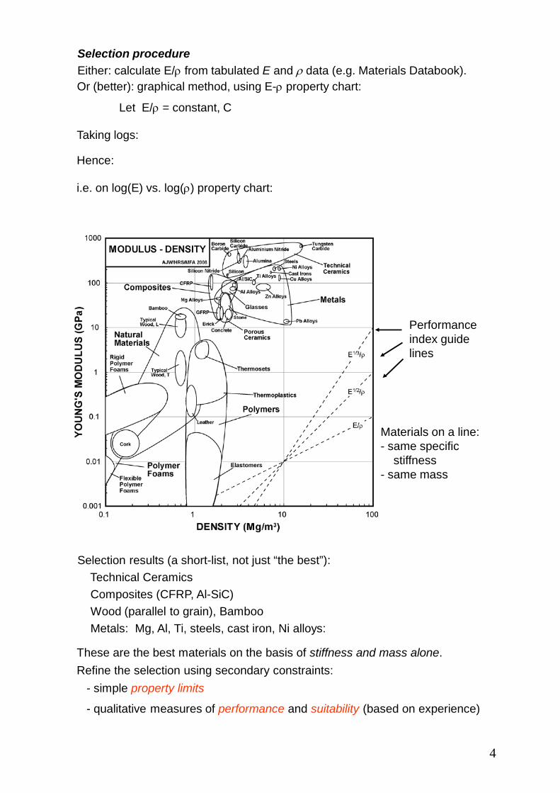
Selection procedureEither: calculate E/ρ from tabulated E and ρ data (e.g. Materials Databook).

Or (better): graphical method, using E-ρ property chart:

Let E/ρ = constant, C

Taking logs:

Hence:

i.e. on log(E) vs. log(ρ) property chart:

Materials on a line:- same specific

stiffness- same mass

Performance index guide lines

Selection results (a short-list, not just “the best”):Technical CeramicsComposites (CFRP, Al-SiC)Wood (parallel to grain), BambooMetals: Mg, Al, Ti, steels, cast iron, Ni alloys:

These are the best materials on the basis of stiffness and mass alone.Refine the selection using secondary constraints:

- simple property limits

- qualitative measures of performance and suitability (based on experience)

4

Secondary constraintsToughness

• numerical criteria for toughness: covered in Easter Term• for now, sufficient to exclude all ceramics from any structural application

(particularly where impact is expected)• same usually goes for glass (though impact-resistant glass can be

manufactured, e.g. windscreens).

Corrosion

• materials must resist chemical attack by the service environment (e.g. water, salt water).

• corrosion is difficult to quantify, depending on subtle details (such as contact between different metals – covered in Easter Term).

• preliminary account of corrosion resistance: - use a simple grading of typical performance in different environments

(e.g. a 5 point scale from very good to very poor)- see Materials Databook, and the CES software

NB: Poor resistance may not exclude a material, but implies the need for protection (e.g. painting), bringing in additional costs. Cost

• product cost includes material and manufacturing cost• as a first indicator: consider material cost only

(“price/kg” bar-chart in Materials Databook)• cost may be an objective (minimum cost) or a constraint (upper limit).

In the tensile tie example, minimum mass was the objective, so we set a limit on material cost (e.g. based on experience with the type of product).

e.g. Cost/kg < £10/kg:

Size / shape / manufacturing limits

Not all materials may be available in the required geometry (e.g. long prismatic sections, thin-walled tubes, I-beams, complex 3D shapes)

This is usually because of manufacturing limits:• Metals and polymers: easy to form into wide range of shapes and sizes:

- casting/moulding (as a liquid)- deformation processing (as a solid or powder)- easy to join (e.g. by welding).

• Ceramics: much more limited, processed by powder compaction. • Fibre composites: difficult to shape; must usually be joined by adhesives. • Wood: some shape limitations;

well-suited to mechanical joining and adhesives.

5

Selection for minimum costExample: cheap, tensile tieObjective now minimum material cost, rather than massFunctional and geometric constraints as before.

Objective: material cost C =

Proceed as before, eliminating free variable A:

Selection:- either use tabulated data for E, ρ, Cm (time-consuming)- or use CES to plot E vs. (ρ Cm), or a bar chart showing E/(ρ Cm)- apply secondary constraints as before (with the exception of cost/kg,

as cost is now the objective, but mass may be a limit instead)

Cost is minimised by maximising the performance index:

Performance indices for light, stiff components in bending

In tension: free variable was area A, but section shape did not matterIn bending: shape is used to improve the flexural rigidity of a given cross-

sectional area of material, e.g. hollow tubes, I-beams etc.Effect of shape: later in the course.

Effect of mode of loading (tension vs. bending) illustrated here via a problem with limited freedom to change the shape: lightweight panel

Example: light, stiff panel in bending

Load, W

Length, L

Width, B

Depth, D

- specified span L, width B- load W in 3-point bending- maximum allowable

deflection, δ- rectangular cross-section,

depth D may be varied

6

Objective: minimum mass

Functional constraint: bending stiffness where IE

LW48

3=δ

12

3DBI =

Geometric constraints: L, B fixed; D variable

Analysis on Examples Paper 3 – resulting performance index is:

On E-ρ property chart:

Short-list of candidate materials (ceramics excluded, due to brittleness)Composites (CFRP, GFRP, Al-SiC) Mg, Al alloysWood, Bamboo, Cork Rigid polymer foams(Glasses)

Apply secondary constraints as before: corrosion, cost, manufacturing.

7

Key points:• significant differences in competition when index changes from E/ρ to E1/3/ρ• use of specific stiffness E/ρ gives non-optimal selection for components

loaded in bending• loading details in bending (e.g. distributed load, cantilever etc) do not

affect the outcome – only the constant in the stiffness equation• best materials can again be identified without numerical values for the

design constants (load, deflection, length)

Footnote:The third guideline on the chart, E1/2/ρ, arises for beams of constant shape(e.g. solid square sections), varying width and depth in proportion.

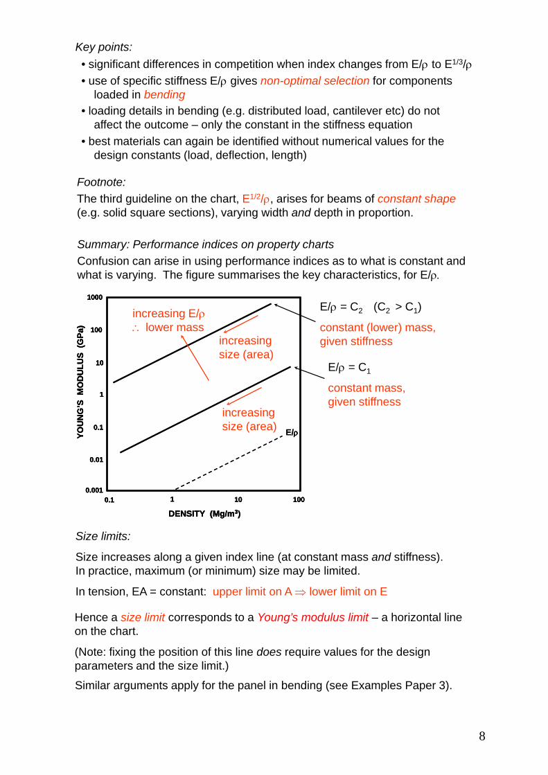
Summary: Performance indices on property chartsConfusion can arise in using performance indices as to what is constant and what is varying. The figure summarises the key characteristics, for E/ρ.

1000

100

10

1

0.1

0.01

0.001

YOU

NG

’S M

OD

ULU

S (G

Pa)

1010.1

DENSITY (Mg/m3)100

E/ρ

1000

100

10

1

0.1

0.01

0.001

YOU

NG

’S M

OD

ULU

S (G

Pa)

1010.1

DENSITY (Mg/m3)100

1000

100

10

1

0.1

0.01

0.001

YOU

NG

’S M

OD

ULU

S (G

Pa)

1010.1

DENSITY (Mg/m3)100

E/ρ

E/ρ = C1

constant mass, given stiffness

E/ρ = C2 (C2 > C1)

constant (lower) mass, given stiffness

increasing size (area)

increasing size (area)

increasing E/ρ∴ lower mass

Size limits:

Size increases along a given index line (at constant mass and stiffness).In practice, maximum (or minimum) size may be limited.

In tension, EA = constant: upper limit on A ⇒ lower limit on E

Hence a size limit corresponds to a Young’s modulus limit – a horizontal line on the chart.

(Note: fixing the position of this line does require values for the design parameters and the size limit.)Similar arguments apply for the panel in bending (see Examples Paper 3).

8

4.3 Introduction to Cambridge Engineering Selector (CES) software

CES is produced by Granta Design Ltd, Cambridge, and embodies this approach to material selection (developed by Prof. M.F. Ashby in CUED).

The software provides:

The Materials Databook tables and property charts are based entirely on CES, so both may be used for problem solving.

The advantage of the software is that many design criteria can easily be imposed together, and the effect of modifying the design requirements can be evaluated automatically and interactively.

• Material property databases

• Material processing databases

• User interfaces for material selection: using property limits, property charts and performance indices

a comprehensive data source for all years of the Tripos

Accessing CES:

CES software is available free to all Engineering students and supervisors, on a time-limited licence (expires end of August).

It requires a good PC, running Windows (not Linux).

Downloadable from Web (CUED PIN protected):

http://www-h.eng.cam.ac.uk/help/engpackages.htmlCES_cut.zip: Level 1+2 databases (sufficient for Part I)CES.zip: Level 1,2+3 databases (larger download – use in Part II)

Download CES_cut.zip, unzip to a directory, and run setup.exe; NB CES requires the .NET framework software: this will install automatically,

if it is not in your version of Windows already)

Do the CES Tutorial and/or follow the audio-video demos, before using CES to do the Examples Paper problems

(Teaching Webpages > First Year Info. > Syllabuses > Paper 2 Materials)

CES also available on PWF, the EIETL computer suite (restricted times), and in some colleges (library or computer room).

9

5. Plastic Properties of Materials5.1 Yielding and strength in design and manufacture5.2 Plastic response of materials5.3 Data for Strength – Material Property Chart

Section 5 covers Examples Paper 3, Q.4-8

5. Plastic Properties of Materials5.1 Yielding and strength in design and manufactureAs the loading on a material or component is increased, the maximum stress reaches the elastic limit. Two types of behaviour may occur:

• Plastic deformation: permanent strain, with the material remaining intact,until internal damage leads to a fracture;

• Fast fracture: cracking across the section – failure is catastrophic, with little or no inelastic deformation (next term).

Strength-limited DesignThe maximum stress a material can carry elastically (its strength) is fundamental in elastic design:

• safe elastic design: find maximum working loads to avoid failure, or size/shape of section needed for a given load (e.g. structures);

• elastic stored energy: elastic deformation stores energy – the strengthdetermines how much (e.g. springs, sports goods);

• maximum elastic strain: strength and stiffness determine the maximum elastic strain (e.g. flexible hinges with large elastic strains; differential thermal strains: may exceed elastic limit).

Plastic deformation is exploited in manufacturing:• deformation processing: many metal shaping processes use large strain

plastic deformation (e.g. forging, extrusion, rolling, machining);• mechanical joining methods: e.g. clinched seams in automotive sheet.

Plasticity in Design and ManufacturingPlastic design requires consideration of loading beyond the elastic limit:

• plastic collapse: design of buildings includes analysis of the mechanismsof plastic collapse (IB Structures);

• plastic energy absorption: deforming a material dissipates energy, as exploited in protection of vehicles (e.g. automotive “crash boxes”, motorway crash barriers).

Plastic deformation also contributes to other failure mechanisms:• fracture: resistance to crack propagation requires energy dissipation –

plasticity at the tip of a crack does this (next term);• creep: at temperatures above 0.4 – 0.5 Tm, materials creep, i.e. deform

slowly and continuously under load (next year).

Plasticity in Design: other failure mechanisms

10

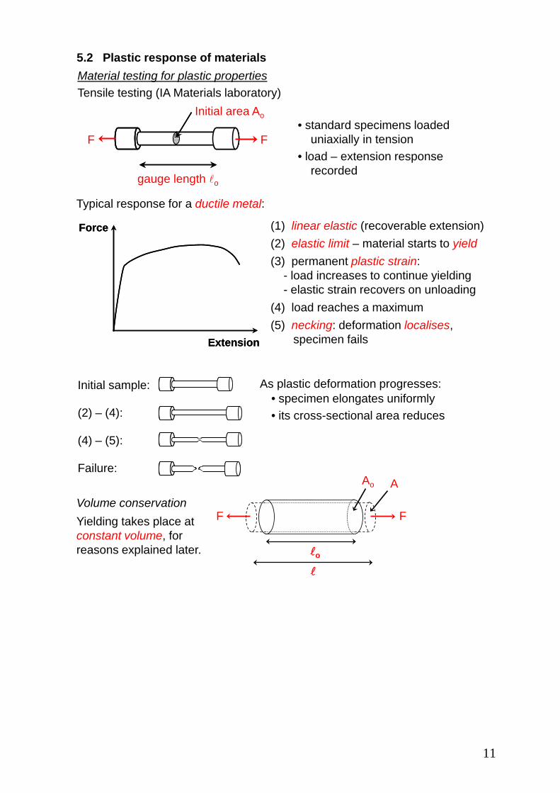
5.2 Plastic response of materials Material testing for plastic propertiesTensile testing (IA Materials laboratory)

• standard specimens loaded uniaxially in tension

• load – extension response recorded

F F

gauge length o

Initial area Ao

Typical response for a ductile metal:

Force

Extension

Force

Extension

(1) linear elastic (recoverable extension)(2) elastic limit – material starts to yield(3) permanent plastic strain:

- load increases to continue yielding- elastic strain recovers on unloading

(4) load reaches a maximum(5) necking: deformation localises,

specimen fails

Initial sample:

(2) – (4):

(4) – (5):

Failure:

As plastic deformation progresses:• specimen elongates uniformly• its cross-sectional area reduces

Volume conservationYielding takes place at constant volume, for reasons explained later.

F

o

F

Ao A

11

Origin of neckingIn region (2 – 4) of the load-extension curve:

• yield load increasing and area decreasing ⇒ actual true stress (F/A) to yield the material is increasing

• increase in resistance to yielding is called work hardening(microstructural origin discussed later)

• this stabilises yielding, so the whole cross-section reduces uniformly

At maximum load , dF/du = 0 (point 4):• the material’s ability to work harden in tension has reduced • at any local narrowing of the section the true stress is higher, but work

hardening is now insufficient to compensate• the plastic strain localises in this section: necking• as the load falls (4 – 5), the sample unloads elastically, but intense strain

in the neck leads to internal damage (voids) and failure

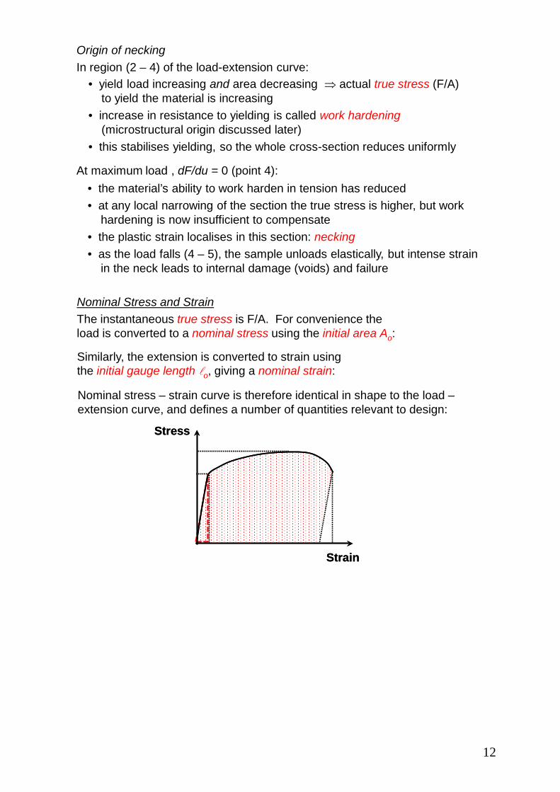
Nominal Stress and StrainThe instantaneous true stress is F/A. For convenience the load is converted to a nominal stress using the initial area Ao:

Similarly, the extension is converted to strain using the initial gauge length o, giving a nominal strain:

Nominal stress – strain curve is therefore identical in shape to the load –extension curve, and defines a number of quantities relevant to design:

Stress

Strain

Stress

Strain

12

Definitions

Yield stress, σy: nominal stress at elastic limit, when yielding starts

Tensile strength, σts: maximum nominal stress in tensile test

Yield strain, εy : σy/E

Elongation (or ductility), εf : permanent strain after failure (i.e. excluding elastic contribution)

Max. elastic stored energy per unit volume: area under linear-elastic region. Stored energy = work done in elastic deformation = ½ Fu.

So stored elastic energy per unit volume

Maximum elastic stored energy per unit volume when σn = σy:

Plastic work per unit volume: area under stress-strain curve (excluding final elastic contribution), i.e. area under force-extension curve divided by initial volume Aoo:

Plastic work/unit volume =

Notes:Yield stress is a material property (does not depend on specimen dimensions)

Tensile strength is mainly useful in comparison with the yield stress – as an indication of the amount of work hardening after initial yield.

Elongation:• includes both the uniform plastic extension up to maximum stress, and the

strain during localisation prior to failure• the latter strain varies with the size of specimen, so elongation is

not a material property• it is still commonly cited as a measure of ductility (e.g. included in CES)• must be treated with caution – acceptable for a first comparison of

materials (provided a standard test has been used)

13

Tensile stress–strain curve variantsSome materials show variants from the standard form illustrated above:Elastic–brittle: No plasticity, ductility = 0

Stress

Strain

XStress

Strain

X Stress

Strain

Stress

Strain

Upper and lower yield point: Short plateau of plastic strain before hardening sets in.

No distinct yield point: Work hardening gives non-linear response from low stresses.The nominal stress at a small plastic strain (e.g. 0.1%) is used to define yield – this is called a 0.1% proof stress, σ0.1. εpl = 0.1%

σ0.1

Nominal stress–strain curves for a range of common alloys (from Materials Databook):

Note on terminology :• Annealed: softened,

by heat treatment• Drawn: previously

hardened, by stretching

Stress–strain curves are significant for manufacturing, as well as design:materials with large tensile ductility (e.g. mild steel, annealed Cu, Al) are easier to form in tension (e.g. wire drawing, deep drawing of cans)

14

Compression TestingIn some circumstances it is preferable to use uniaxial compression:

• Ceramics: tend to fracture in tension (from internal flaws); much stronger in compression, and may yield (particularly when hot)

• Metals: if unavailable in suitable geometry for tension.

Nominal stress:

Nominal strain:

Area increases during test – load for yielding rises(due to larger area, and due to work hardening).

Localisation and necking do not occur – the test geometry is stable.

F

ho h

F

F

ho h

F

Ao A

Constant volume = Ao ho = A h

HardnessTension and compression tests are destructive – samples are machined to size and tested to destruction. It is often desirable to use non-destructive testing (NDT):

• may need to return component to service after testing• size/shape may not allow manufacture of tensile or compressive sample• tensile/compression testing can be expensive and time-consuming

Hardness test – standard low-cost NDT technique for measuring strength:

• diamond pyramid is pressed into the surface under a constant load;

• local plastic deformation occurs until load is supported;

Hardness defined as:

Units: usually kg/mm2

(can also be expressed in MPa: multiply by g, acceleration due to gravity).

F

Projected area A

d

F

Projected area A

d

e.g. Vickers hardness test

e.g. Vickers hardness, “HV5” (i.e. load, F = 5 kg): conversion from d to HVtabulated for standard loads.

• load removed and the resulting indent size, d, is measured;

• A = (d/√2)2 = d2/2

15

• average strain is of the order of 8%, so the hardness relates to the yield stress at this strain

• hardness (in MPa) is approximately equal to 3 × yield stress, H ≈ 3σy

Relationship between hardness and yield stressUnder the indenter, a steep strain gradient exists – the deformation and work hardening is greatest near the indenter. Plastic analysis indicates that:

e.g. low carbon steel:

True Stress and StrainNominal stress and strain are convenient for material testing, but do not take account of changes in geometry. In some circumstances it is preferable to account for geometry correctly, and to use true stress and true strain: True StressFor uniaxial load, true stress is: and nominal stress is:

AF

t =σo

n AF

=σ

For constant volume (i.e. for plastic deformation): AA oo =

Hence:

Nominal strain: nooo

on ei ε+=−=

−=ε 1..,1

Hence: i.e. true stress > nominal stress (for εn > 0).

True stress is easily calculated from nominal stress–strain data, but only as far as the onset of necking in tension (deformation no longer uniform) –the continuation of the true stress–strain curve must be found in compression.

True StrainTrue strain is more difficult to visualise – each increment of extension dis divided by the current length (not the initial value), to give an increment of true strain: /dd =εTotal true strain is found by integrating between original and final lengths:

==ε ∫

oot

d

ln

Since: , true strain is: )1( no

ε+=

i.e. true strain < nominal strain (for εn > 0), and easily calculated from εn.

16

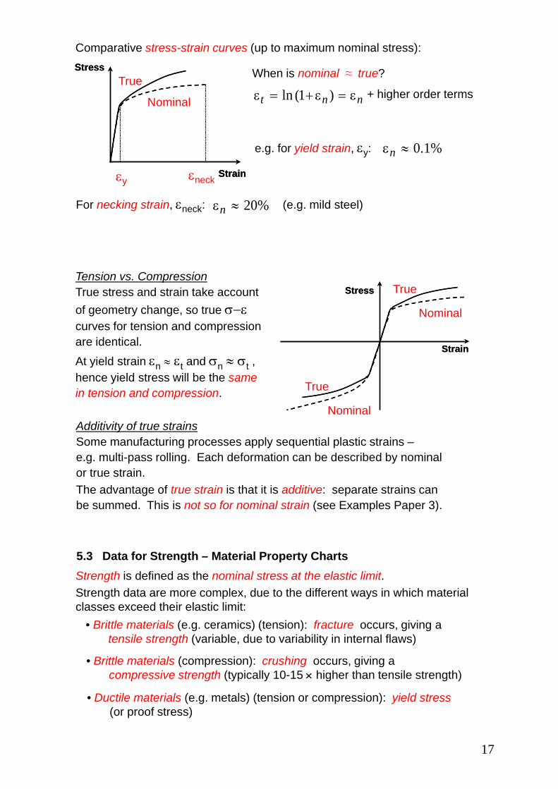
Comparative stress-strain curves (up to maximum nominal stress): Stress

Strain

Stress

Strain

True

Nominal

εneckεy

When is nominal ≈ true?

nnt ε=ε+=ε )1(ln + higher order terms

e.g. for yield strain, εy: %1.0≈εn

For necking strain, εneck: (e.g. mild steel) %20≈εn

Tension vs. CompressionTrue stress and strain take account of geometry change, so true σ−εcurves for tension and compression are identical.At yield strain εn ≈ εt and σn ≈ σt , hence yield stress will be the same in tension and compression.

Strain

Stress

Strain

Stress

True

Nominal

True

Nominal

Additivity of true strainsSome manufacturing processes apply sequential plastic strains –e.g. multi-pass rolling. Each deformation can be described by nominal or true strain. The advantage of true strain is that it is additive: separate strains can be summed. This is not so for nominal strain (see Examples Paper 3).

5.3 Data for Strength – Material Property Charts Strength is defined as the nominal stress at the elastic limit. Strength data are more complex, due to the different ways in which material classes exceed their elastic limit:

• Brittle materials (e.g. ceramics) (tension): fracture occurs, giving a tensile strength (variable, due to variability in internal flaws)

• Brittle materials (compression): crushing occurs, giving a compressive strength (typically 10-15 × higher than tensile strength)

• Ductile materials (e.g. metals) (tension or compression): yield stress(or proof stress)

17

Material property charts including Strength

NB: Envelope round technical ceramics, glasses and porousceramics shown dotted: data for compression only

(1) Strength vs. Density

Performance indices –return to these later.

Notes:

• Strength for solid materials spans over 3 orders of magnitude – natural materials and polymer foams extend the range to much lower strengths;

• Metals, ceramics and composites are the strongest materials, but there is some overlap with polymers;

• Individual classes of metals (e.g. steels, Ti alloys etc) cover much wider ranges of strength than is observed for Young’s modulus or density.

NB. Wide ranges in strength but not in Young’s modulus –strength is a property that can be manipulated widely by composition and processing.

(2) Young’s Modulus vs. Strength

Further performance indices – e.g. yield strain, elastic stored energy per unit volume

Materials Databook also includes a property chart for Fracture Toughness vs. Strength – discussed in the Easter Term lectures on fracture.

18