B TECHNICAL RPR

' NO. lI J

[ I1

I¢

i' DYNAMIC ANALYSIS AND DESIGN OF CONSTRAINED

MECHANICAL SYSTEMS E

Interim Report OEC

12 June 1981

Contract No. DAAK30-78-C-0096

Edward J. Haug, Roger Wehageand N.C. Barman

College of EngineeringThe University of IowaUniversity of Iowa Rept. No. 50

yRonald R. Beek, Project Engineer, TACO0ii

i Approved for public release; distribution unlimited.

L ... . . . . . . . . . . . .

U.S. ARMY TANK-AUTOMOTIVE COMMANDRESEARCH AND DEVELOPMENT CENTERWarren, Michigan 48090

81 12 17066-

DISCLAIMER NOTICE

THIS DOCUMENT IS BEST QUALITYPRACTICABLE. THE COPY FURNISHEDTO DTIC CONTAINED A SIGNIFICANTNUMBER OF PAGES WHICH DO NOTREPRODUCE LEGIBLY.

.4,

NOTICES

The findings in this report are not to be construed as an official Department

of the Army position.

Mention of any trade names or manufacturers in this report shall not be

"construed as advertising nor as an official endorsement of approval of such

products or companies by the U.S. Government.

Destroy this report when it is no longer needed. Do not return it to

originator.

-74 R

SA-

UNCLASSIFIEDSECURITY CLASSIFICATION OF THIS PAGE (Man Oat Entered)

PAGE READ INSTRUCTIONSREPORT DOCUMENTATION PBEFORE COMPLETING FORM

I. REPORT NUMBER OVT ACCESSION NO. 3. RECIPIENT'S CATALOG NUMBER

12588 /- J 6J$4. TITLE (and Subtitle) 5. TYPE OF REPORT & PERIOD COVERED

Dynamic Analysis and Design of Interim to Nov. 78

Constrained Mechanical Systems 6. PERFORMING ORG. REPORT NUMBER

7. AUTHOR(*) S. CONTRACT OR GRANT NUMBER(a)

Edward J. Haug, Roger Wehage & N.C. BarmanUniversity of Iowa DAAK30-78-C-0096Ronald R. Beck- TACOM

9. PERFORMING ORGANIZATION NAME AND ADDRESS 10. PROGRAM ELEMENT. PROJECT, TASKAREA & WORK UNIT NUMBERS

The University of IowaCollege of EngineeringIowa City. IA 52242

11. CONTROLLING OFFICE NAME AND ADDRESS 12. REPORT DATE

US Army Tank-Automotive Command R&D Center 12 June 1981

Tank-Automotive Concepts Lab, DRSTA-ZSA 13. NUMBER OF PAGES

Warren. MI 480905514. MONITORING AGENCY NAME & ADORESS(if diformt from Controlling Office) IS. SECURITY CLASS. (of thl report)

UNCLASSIFIED

ISa. OECLASSIFICATION/DOWNGRADINGSCHEDULE

16. DISTRIBUTION STATEMENT (of thl Report)

Approved for public release; distribution unlimited.

17. DISTRIBUTION STATEMENT (of the abtraet entored in Block 20. It different from Report)

1. SUPPLEMENTARY NOTES

19. KEY WORDS (Continue on reverse aide if nececsary mud Identify by block number)

Dynamics, Bodies, Response, Control, Interaction, Stability, LagrangianFunction, Matrices

24 AI'TACT (*faue M revers nme -, sell tf by block numbee)

A method for formulating and automatically integrating the equations of motionof quite general constrained dynamic systems is presented. Design sensitivityanalysis is also carried out using a state space method that has been usedextensively in structural design optimization. Both dynamic analysis and designsensitivity analysis and optimization are shown to be well-suited to applicationof efficient sparse matrix computational methods. Numerical integration iscarried out using a stiff numerical integration method that treats mixed systems

D OR W3 Eorno OF" v NO S S L / / iSECURITY CLASSIFICATION OF THIS PAGE (Wham Date Entered)

I _"_ni - -J '*. .

UJNCLASS IFIEDSECURITY CLASIFICATION OF THIS PAOI(WMa. Date BatweQ

of differential and algebraic equations. A computer code that implements themethod of planar systems is outlined and a numerical example is treated. Thedynamic response of a classical slider-crank is analyzed and its design isoptimized..

SECURITY CLASSIFICATION OF THIS P9AGE1Uen Date Entered)

W, I I-

ABSTRACT

A method of formulating and automatically integrating the equations

of motion of quite general constrained dynamic systems is presented.

Design sensitivity analysis is also carried out using a state space method

that has been used extensively in structural design optimization. Both

dynamic analysis and design sensitivity analysis and optimization are

shown to be well-suited to application of efficient sparse matrix computa-

tional methods. Numerical integration is carried out using a stiff

numerical integration method that treats mixed systems of differential

and algebraic equations. A computer code that implements the method for

planar systems is outlined and a numerical example is treated. The dynamic

response of a classical slider-crank is analyzed and its design is

optimized.Aocession For

NTIS GRA&IDTIC TABUnannounced

Justification

Distribution/

Availability CodesjAvail and/or

Dist Special

Li

ii

-r/

I. Introduction to Computational Dynamics

Computational methods for dynamic analysis of electronic circuits [1]

and structures [2] have become well developed and user-oriented, a situation

that is not enjoyed in the field of mechanical system dynamics. In most

areas of mechanical design, classical Lagrangian methods of dynamic analysis

are still used almost exclusively. It is the purpose of this paper to

present an integrated method of constrained mechanical system dynamic

analysis and design sensitivity analysis that is user oriented and capable

of routine application to large scale systems.

Development of general purpose computed codes for dynamic analysis

of mechanisms and mechanical systems are initiated in the mid-1960's and

has made significant progress for certain classes of mechanical systems.

A comprehensive survey of computer codes and the analytical techniques on

which they are based has been presented by Paul [3]. He cites numerous

planar (2-D) mechanism analysis codes, but only two three-dimensional (3-D)

analysis codes. At the present time only the 3-D Integrated Mechanism

Program (IMP) [41 and the 2-D Dynamic Response of Articulated Machinery

(DRAM) [5] codes are well developed and user-oriented. However, they are

both based on closed loop linkages or mechanisms, which is too restrictive

a class for general use in mechanical system dynamic analysis and design.

A general 3-dimensional Automatic Dynamic Analysis of Mechanical Systems

(ADAMS) method [6] has been presented that is fundamentally better suited

for dynamic analysis of systems that are not in closed loop configurations.

However, no generally applicable computer code is available at the

present time. The ADAMS modelling method is all the more attractive

since it is well-suited for extension to design sensitivity analysis.

L LI

2

Before presenting the theory it is helpful to constrast two funda-

mentally different approaches to modelling linkages and mechanical systems

that are presently in use. The loop closure method generates equations

that require closure of each independent loop of the linkage. The

resulting nonlinear equations are then differentiated to obtain the

smallest possible number of independent equations of motion, in terms of

a minimum number of system degrees of freedom. Thus, the loop closure

method generates a small number of highly nonlinear equations that are

solved with standard numerical integration methods. The constrained

system modelling method, on the other hand, explicitly treats three

degrees of freedom for each element of the system (in the plane).

Algebraic equations prescribing constraints between the various bodies

are then written and elementary forms of equations of motion for each

body are written separately. The constraint equations prescribing

assembly of the mechanism are adjoined to the equations of motion through

use of Lagrange multipliers. Thus, one treats a large number of equations

in many variables. These equations may be solved by an implicit numerical

integration method [1] that iteratively solves a linear matrix equation.

The saving grace of this technique is that the matrix that arises in the

iterative solution process is sparse. That is, only three to ten percent

of the elements of the matrix are different from zero.

It is the purpose of this paper to develop the theory of dynamic and

design sensitivity analysis and to present a computer code called Dynamic

Analysis and Design System (DADS) that implements the constrained system

modelling method for planar systems. The same basic theory is applicable

for three-dimensional systems, but due to analytical complexity it will be

presented in a separate paper.

- *: L *

,... .

2. Constrained Equations of Planar Motion

For planar mechanical systems, constraints between elements are taken

as friction free (workless) translational and rotational joints. Exten-

sions to include constraints such as cams, prescribed functional relations,

and intermittent motion are possible by incorporating provisions for non-

standard elements that are supplied by the user. In addition to standard

constraints, springs and dampers connecting any pair of points on different

bodies of the system are included in the model. In addition to these

standard force elements, allowance is made for external forcing functions.

Generalized Coordinates: In order to specify the configuration or

state of a planar mechanical system, it is first necessary to define

generalized coordiates that specify the location of each body. As shown

in Fig. 2.1, let the x-y coordinate system be an inertial reference frame.

Define a body fixed coordinate system i - ni embedded in body i, with

its origin at the center of mass. One can now locate the rigid body i by

specifying the global coordinates (xiYi) of the origin of the body fixed

coordinates and the angle *i of rotation of this sytem relative to the

global coordinates.

Let p be a point on body i, as shown in Fig. 2.1. The coordinates

of the point in the body fixed i - ni system are i and niP. The same

point may also be located by its global coordinates x P and yip . The

relation between these coordinates is

= + E(*i) [ (2.1)

y -

p yi1

4

where E(Oi) is the transformation matrix

cos *i- sinE(0 C) 1 (2.2)

i I-Lsin i cos iJ

In terms of these generalized coordinates, one can write the kinetic

energy of the ith body as

1 .2 .2 1 *2(23KE i =mi(Xi +yi)+ Ji i (2.3)

where mi is the mass of the ith body and Ji is its centroidal polar

moment of inertia.

Further, one can write the virtual work of all externally applied

forces on body i as

6We - i 6xi + Qyi 6Y + Q i 6 (2.4)

The effect of all forces except the workless constraint forces between

bodies is included on 6W of Eq. 2.4.e

Equations of Constraint: Figure 2.2 depicts two adjacent bodies i

and J. The origins of their body fixed coordinate systems are located by

the vectors Ri and R with respect to the inertial frame of reference.

Let an arbitrary point Pij on body i be located by rii and pJi on body j

be located by rj1. These points are in turn connected by a vector rji- P*

One can write a vector equation beginning at the origin of the inertial

reference frame and closing there, to obtain the vector relationship

R i + rid +rp -rji -Ri (2.5)

i i .p .j

5

The constraint equations for a revolute joint are now obtained by re-

quiring that Pij and pji coincide. Setting r = 0 and writing Eq. 2.5 inP

component form, one has

x + %. ijCos 01- n sin 0 i - x3 - ciCos 0 + n isin 0

Yi + &ij sin i + nij cos Oi - Y - Ei sin 0 - nji cos = (2.6)

For a translational joint shown in Fig. 2.3, let points pij and p..

lie on some line parallel to the path of relative motion between the two

bodies. In addition, let them be located such that rij and rji are per-

pendicular to this line and of nonzero magnitude. Successively forming

the dot product of Eq. 2.5 with rij and ri and adding, one obtains the

scalar equation

- - 2 2 rrij ji + ri + rij i Ri rij - i i+ i j

(2.7)

which reduces to

( ij cos i - ij sin i + Eji cos - )ji sin 4 ) (xi - x )

+ (CiJ sin 4 i+flij cos i+ jisin j+n jicos 01)(Yi- Y )

2 2 2 2+ ij + nij -ji n nji = 0 (2.8)

A second scalar equation is obtained by noting the r i x -"Ji 0. Expan-

sion of the cross product yields only a z component, which must be zero.

This is

IA

6

(ij Cos * i - sin *i)(&ji sin i + nji cos )

- ( J cos j- riji sin t1j) (ij sin 0i + nij Cos i 0 (2.9)

Spring-Dampers: Since springs and dampers generally appear in pairs,

they are incorporated into a single set of equations. If one or the other

is absent, its effect is eliminated by setting that term to zero. The

equations for spring-damper force and torque are

[k (Z ) + c~ v~ + FO~~ -R (2.10)Fij ij( iJ -, 0i j cij vi Fij] Lij Sij

T -k (0ij )+ c +T (2.11)ii rij ij 00i r ij j 0i

ri -€j i j 0ij

where

Fi. is the resultant force vector [F ,Fyij]T in the spring-ijx yj

damper

TR is the vector [xij cos a, lij sin a] between pointssij

Sij and S of a spring-damper connection on the two

bodies, as in Fig. 2.4

Tij is the torque acting on two bodies at a revolute joint

kij and k are elastic spring coeffientsijl

c and c are damping coefficientsij r ij

I0 and are the undeformed spring length and angular0 ij 0i

rotation in the revolute

xij and *ij are the deformed spring length and angular

rotation in the revolute, and vij and ;,J are the time

derivatives of £iJ and ijiiojI E

7

F and T are constant forces and torques applied along01ij 0 ijthe spring and around the revolute joint between two

bodies

From Fig. 2.4 a vector expression similar to Eq. 2.5 is written as

R + r +R -r -. 0sij sij Sji J

or in component form

.ij i 5.. "i

13 Z .L.~ s i n 2 Y s i n . + ;n c o s

13S j I j

xj rsji cos 4j n s ji n

+ + (2.12)

L sin + si cos j

where a is the angle between R and the inertial x axis. Equation 2.12sic

is used to obtain Z.. by noting that

ij = [(Z ij cos ct) 2 + (k.ij sin a)2] 1 / 2

= [(-xi - cos 4i + n sin 4i + x +s Cos 4jsii i s J ji c

sin 2' + (- S sin n' s] Cos2.1

+ Y + s sin J + cos 4C)s 2 1/2 (2.13)

'.I.. . . .... T : : .- ", , .

,. ., . ,

. I,-. ,, L •

8

Substituting the left side of Eq. 2.12 into Eq. 2.10, the following force

expressions are obtained:

F lFI cos a (2.14)

F =,.j IF I sin a (2.15)yij ii

where cos a and sin a are obtained by dividing Eq. 2.12 by Lij. Finally,

defining

V =j - j (2.16)vij

and transfering Zij, F , F , and v.. to the right hand sides of Eqs.xij yij 1J

2.13 to 2.16, one obtains equations in the form required by the numerical

integration algorithm.

System Equations of Motion: With the kinetic energy given by Eq.

2.3 and the generalized forces associated with externally applied forces

and spring-dampers, one can construct the equations of motion for the

system. To allow for a unified development, let q denote the vector

[xi,yi,oi IT of generalized coordinates of body i. Denote the kinetic

energy of body i as KEi(q ), the generalized force on body i as Q i(q i),

and the equations of constraint between bodies i and j as ij(qi qj) = 0,

i < J. Here the constraint numbering convention is that i < j in order

to preclude inclusion of the same set of constraint equations twice.

Presuming that the constraints are workless, one has the variational

equation of motion [7]

-.,

9

dt - 6q Q Q 6iO (2.17)

that must hold for all time and for all virtual displacements 6q that are

consistent with the constraints. This is

3ij i j s6i Sq + i qj = 0 i < j (2.18)

3q I qj

By the Farkas Lemmas of optimization theory [9], there exist multipliers

Xij, i < j, such that

S T ij

6q. ( 1 1 Q6q 3+ I XT ij aq -q q 0 (2.19))iq- t aq1

Ui 1 1 i~ i

for all 6qi By Eq. 2.3, KEi =1 Mq, where2

= in 0 0

0 0

and Eq. 2.19 may be written in the form

iTM -i* XqjT aq+ = 0 (2.20)i ~ q J<i D i

Since Eq. 2.20 must hold for arbitrary 6qi, this yields the equations

of motion

Mi.i _ Qiq)+ I i i I $ji

Q(q ) +. - ii+ X = 0 , i1,... ,r (2.21)i<j q j<i 3q

- , t,,,_-..______.._. ,.,.

10

These differential equations and the algebraic constraint equations

Pij(qi,qj) = 0 , i < j (2.22)

form the system equations of motion. Defining the generalized velocity

vector

i "iu = q

one can replace the second order system of Eqs. 2.21 by the first order

system

Mini Qi (qi) + O ij + xji - 0 (2.23)i<j i q j<i 3q

q - u - 0 (2.24)

The problem of dynamic analysis is thus reduced to solving the

system of differential and algebraic equations of Eqs. 2.22 to 2.24, with

initial conditions given that are consistent with the constraints of Eqs.

i i i2.22. The solution variables are q and ui, i-i,...,r and X for all

i < j. Each of these variables is a function of time.

- I .. * i.

3. Integration of Constrained Equations of Motion

Numerical Integration of Differential Equations: In order to solve

the differential equations of motion, numerical integration theory must

be used to obtain a set of approximations that are suitable for digital

computation. Integration of the equations of motion must be accomplished

as asimultaneous solution of the algebraic and differential equations of

Eqs. 2.22 to 2.24. Standard numerical methods are however designed to

solve only systems of differential equations of the form

= f(y,t) (3.1)

where y is an m-vector of unknowns and f is an m-vector of known functions.

A modified approach is taken here that allows for the simultaneous solution

of mixed algebraic and differential equations of the form

g(y,y,t) = 0 (3.2)

where some components of y may not appear in any of the equations, or they

may appear nonlinearly. Before introducing the method to be used, it is

instructive to review the approach applied in solving Eq. 3.1.

The basic method of constructing approximate solutions [I] is to

place a time grid ti, i=l,... on the interval [O,T], where hi = t i+ - ti

is the grid spacing. One then approximates the solution y(t) of Eq. 3.1

on the time grid as y Y(t

The basic approximating equation for stiff differential equations [1],

i.e. differential equations with widely split eigenvalues, is the Gear

algorithm

* *2e, - . . .+L . . . . . ... .. . -. ' .- . '. -. , K :

12

ki+l •iil i-J +i-y yj 0 - y (3.3)j-1

where the constants 80 and mi, J-1,..., k, called Gear's coefficients, are

determined so that Eq. 3.3 is exact for any polynomial solution of Eq. 3.1

of degree up to k. Gear's coefficients [1] also have the propercy that

the algorithm tends to be stable, even for stiff differential equations.

The multistep formula that is used to solve Eq. 3.2 is derived from

Eq. 3.3. One progresses from ti to ti+ 1 by solving Eq. 3.3, together with

i+ i+1l34

g(y , y , ti+1) 0 (3.4)

Linearization of Eq. 3.4 generates the Newton formula

(m) a(m) .(n myy + a- g (3.5)

where Ay(m ) . y(m+l) _ y(m) and m represents the iteration number. The

time step index i has been suppressed here for notational simplicity. Sub-

stitution of Eq. 3.5 into Eq. 3.3, noting that the summation term of Eq.

3.3 remains constant at each iteration, yields the corrector formulas

a~i) ag(m) A(in) (m)10-0 y + Dy J y (3.6)

A (m) Ay (m ) (3.7)

h80

If Eq. 3.2 is of the form Pj + f(y,t) 0 0, then Eq. 3.6 is of the

form

.4

13

h_ a 3f (m)" y(m ) (m)-e + -ay = - m (3.8)

The iterative corrector procedure is continued at each time step until

all of the Newton differences Ay (m ) are below a specified tolerance level.

At each iteration y and y are updated as

y(m+l) M y(m) + Ay(m)

*( -l (m) *(m) (Cm) 1 __A (in)y =y + Ay =y ~

0

It is interesting to note that every element of y is obtained at each

time step, even though many elemerLts of y may not appear in any of the

equations.

Sparse Matrix Algebra: The sytem of nonlinear algebraic and differ-

ential equations defined in the previous paragraphs is very loosely

coupled. For two reasons, no attempt is made to eliminate variables to

obtain a smaller system of equations. First, the Jacobian matrix that is

formed by linearization of the loosely coupled equations and used in

iterative solution by Newton's method is sparse and can be very efficiently

stored and decomposed. Second, the repetitive nature of the loosely

coupled equations results in compact and efficient computer routines for

evaluating the nonlinear equations and nonzero matrix entries. Recently

developed sparse matrix algorithms [8] make both of these operations

practical and desirable. It has been shown [8] that it is usually more

efficient to solve large systems of sparse equations, rather than smaller

systems with greater percentages of nonzero entries.

.......................................................................................

I - .1.

14

Consideration of matrix sparsity is important to the speed of computa-

tion in problems of dynamic system analysis [1]. When less than 30% of the

matrix entries are nonzero, it is inefficient to store the matrix as a full

two-dimensional array. Instead, only the nonzero entries are stored in

compacted form. The method most commonly used for compacting the data is

to store the row and column indices of each nonzero-valued entry in the

matrix in two vectors I and J and the value in a third vector A. This is

called "i-j" ordering.

Sparse matrix algorithms are most efficient when the nonzero matrix

entries are stored in an organized manner. This usually implies that they

be evaluated row by row or column by column. The previously mentioned

repetitive matrix evaluation scheme is defeated by this requirement, since

it usually results in the evaluation of small submatrices located at

various positions throughout the matrix. To overcome this difficulty, a

permutation vector is generated from the row and column vectors describing

the nonzero-valued positions. As each matrix entry is generated, it is

directed to a specific location in the "A" vector by a permutation index.

At completion of the matrix evaluation, all entries are stored exactly

as if they had been evaluated in column order.

A sparse matrix decomposition algorithm is then applied to the column

ordered matrix and an LU factorization [1] is accomplished. Full pivoting

is not achieved, but the algorithm chooses, from among the largest of the

acceptable pivot elements, the pivot that results in a minimum number of

fills in the resulting L and U matrices. This is important for efficient

execution of the forward and backward substitution phases, since an in-

creased number of fills destroys the original matrix sparsity and results

in excessive computer time.

_Z m A

15

4. Elements of Design Sensitivity Analysis and Optimization

As shown in this section and developed in more detail in companion

papers [91, the constrained dynamic system model of Section 2 and the

implicit numerical integration formulation of Section 3 are ideally suited

for efficient design sensitivity analysis. If the designer identifies a

set of parameters b = [b1,...,b IT that he uses to specify the system

design, a natural question that arises is: How does a design variation

6b - [ib .... ,6b T effect the dynamic response of the system? An even

more important question is: What is the effect on dynamic response of a

design variation 6b that is required to be consistent with certain per-

formance requirements? A method of design sensitivity analysis developed

for related classes of problems [10] is employed here to answer these

questions.

In order to address the design sensitivity analysis problem, a compact

Tnotation is required. Let the vectors z(t) = [z1 (t). ....,Zm(t)] contain

all generalized displacement and velocity coordinates;

Z(t) = [ 1 (t),) ,t), .... I1 contain spring lengths, velocities and forces;

ij r Tand X(t) = [A (t), i < j contain Lagrange multipliers that are

associated with constraints (which determine reaction forces associated

with constraints).

With this notation, the equations of motion are written in compact

form as

P(b)z + f(t,z,X,Z,b) 0(4.1)

z(O) = v(b)

The matrix P is made up of 6 x 6 matrices that are associated with

16

derivative terms in Eqs. 2.23 and 2.24 for each of the bodies; i.e.,

Pi(b) - diag (mi(b), mi(b), Ji(b), 1, 1, 1). Similarly, the vectori

fi is made up of the remaining terms in Eqs. 2.23 and 2.24; i.e.,

(i Q I ¢0j Xi -I -ji 'jl)

[_ xi i j a i {i ax '

0i- Xij - Zaji Xji)

y i<j Yi j<1 yi

at X#ij _ ,j Xji) ,uit vis wil T

0 i<j -i i J<i 3i

The spring damper equations of Eqs. 2.13 to 2.16 in matrix form are

i + e(z,Z,b) - 0

(0) . . . !(4 .2)- l~(b), j - 0,1,. ,s-i(42

£1+4jJ l

where s is the number of spring damper pairs and the matrix I is diagonal

and contains all zeros, except for ones on the diagonal corresponding to

coefficients of iij in Eq. 2.16. The vector 8 simply contains all other

terms of Eqs. 2.13 to 2.16.

Finally, the set of kinematic constraints is written in vector form as

O(z,b) 0 (4.3)

I.

The dependence of Eqs. 4.1 to 4.3 on the design variable b represents the Vfact that b may include such parameters as spring and joint locations,

spring and damper coefficients, masses, and moments of inertia.

Optimal Design Problem Formulation: For the purpose of this intro-

ductory discussion of design sensitivity analysis, the cost function to

6B

17

be minimized and performance constraints to be satisfied are taken in

integral form. The general design problem is then to minimize

g0 = (b) + L0 (tzA, ,b)dt (4.4)0 0f

subject to the constraints

IT 0, il ..rSi gi(b) + Li(t'z' A'Zb)dt < 0 i=1 ,...,r (4.5)

01 0,i=r'+l,. .... r

This form of integral constraint can be made to include constraints

that must hold for all time; i.e.,

n(t,z (t),X(t),L(t),b) < 0 , 0 < t < T (4.6)

The inequality of Eq. 4.6 is equivalent to the integral constraint

I [n(t,z(t),A(t),X(t),b) + ln(t,z(t),X(t),i(t),b)I]dt = 0

which is of the form of Eq. 4.5. This technique has been used for a wide

variety of constrained dynamic systems [11] with good success. It may be

noted that constraints of the form of Eq. 4.6 may represent excursion

limits, bounds on stress, path generation error bounds, and a multitude

of other forms of meaningful design constraints.

Design Sensitivity Analysis: In order to determine the effect of a

design variation 6b, one must first note that the solution of Eqs. 4.1

to 4.3 will be changed by perturbations 6z, 6X, and 6X. Presuming the

design problem is well posed, small perturbations 6b in b will lead to

small perturbations in the solution variables.

18

Consider a typical functional of Eq. 4.4 or 4.5 where the subscript

has been deleted for notational simplicity. To first order, one has

+6A a a+L 6Z + 6b dt (4.7)

ab JO 9Z a az 3b

The objective is to eliminate explicit dependence of Eq. 4.7 on 6z, 6X,

and 61 and to write 60 explicitly in terms of 6b. To do this, an effective*

technique is to introduce adjoint variables 1, p', and * , multiplying

Eqs. 4.1 to 4.3 respectively, and integrate to obtain the identities

J T[P(b)z + f(t,z, X,2,b)]}dt = 0

f{W [IT[i + e(z,I,b)]}dt - 0 (4.8)

f *oI *T.(z,b) }dt -0

Then integrate Eqs. 4.8 by parts and require that 1, i', and u* satisfy

the adjoint equations

T afT asT aeT _, _ aLT

;fT a+ T ,* aLT (4.9)

azat at(49

as - a. L=-0az 3 T

and terminal conditions

tI.

19

W(T) 0,W ' (T) 0, W*(T) = 0 (4. O)

The funcational 64 may then be rewritten as

S= = AT Sb (4.11)

where

av s-i

AT = + - rT(o )P (b) L + , 1 VI 0)

j=0 b14j 3b

- b - P- f T b T dt (4.12)

One may now integrate the differential equations 4.9 from r to 0,

using the terminal conditions of Eq. 4.10. If one uses the implicit

numerical algorithm of Eq. 3.8 for the above set of equations, the Newton

iteration formula is

( P T+ iifT) ae T a0T]F

3fT ( eT T0 AU' -- g (4.13)

0 0

where g represents the left hand side of Eq. 4.9. For ready reference, it

is desirable to repeat Eq. 3.8 applied to Eqs. 4.1 to 4.3 here asT T

!+

-L 0 .4.1.

at .. .. . .. . .. ... . .. . .. . .. . .. .

20

/1 af _P T_ip + _L A-z -

3z i - 0 At - g (4.14)

az 3Z

aD0 0 A

where g represents the left-hand side of Eqs. 4.1 to 4.3.

Note that the coefficient matrix in Eq. 4.13 is exactly the transpose

of the matrix of Eq. 4.14 with the exception of the (-l/h 0) term. But

since one integrates from r to 0, this implies negative time steps h, hence

one need not modify the expressions (1/ho0 P +'Lf) and (1/hB 1 + _y) of

Eq. 4.14 for use in Eq. 4.13. Thus, one can use the same sparse matrix

factorization code generated for dynamic analysis to solve Eq. 4.13 during

adjoint calculations. The numerical efficiencies are obvious. This entire

subject is addressed in detail in Ref. 9.

Method of Generalized Steepest Descent: The linearized optimal

design problem is to find a vector 6b that minimizesOT

610 - A 6b (4.15)

subject to design constraints

T ( - *V,81, .. ,r'

6* = A 6b (4.16)- @8 (r'+l.... ,r), *8 > -

and the quadratic step-size constraint

6bTw6b < 2 (4.17)

I. .. ~ L

21

where $ is a vector of c-active constraints, A contains sensitivity coef-

ficients associated with e-active constraints, W is a positive definite

weighting matrix, and and E are small positive numbers.

Employing the Kuhn-Tucker necessary conditions of nonlinear program-

ming [11], one derives the necessary design change 6b as

6b=- 6b + 6b2 (4.18)

where

2 -1 - 26b = -W A y (4.20)

M y1 = _TW-1 AO (4.21)

M 2 - (4.22)M T -1-

M =r W- (4.23)

1 1and -i > 0 is to be chosen as a step-size. The vector 6b is a constrained0 22"(

design derivative and 6b2 is a vector design change that corrects constraint

errors.

..... .... ' , ll

22

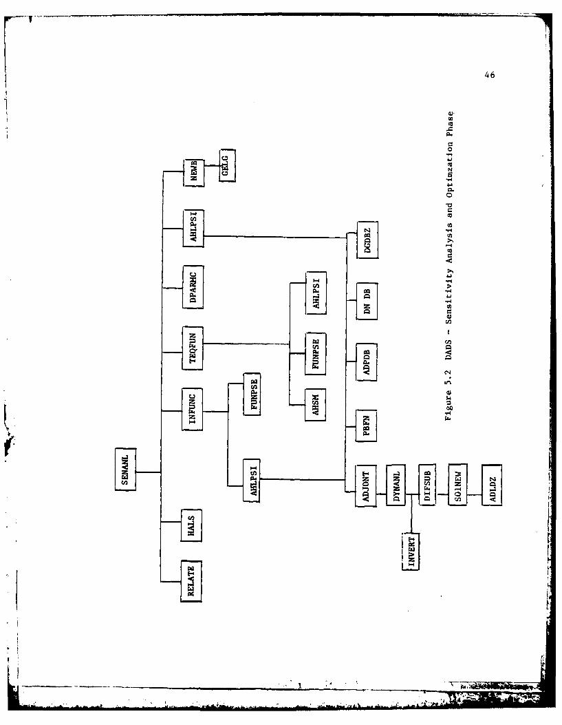
5. Dynamic Analysis and Design System (DADS)

The DADS computer program implements the dynamic ana.ysis, sensitivity

analysis, and optimal design methods presented in Sections 2 to 4.

Figures 5.1 and 5.2 are diagrams showing the subprograms that are used

for dynamic and sensitivity analysis. Figure 5.3 gives the overall program

flow diagram that incorporates these subprograms.

The dynamic analysis phase (DYNANL) of the program generates sparse

matrix code for pivoting and LU factorization and solves the system of

differential - algebraic equations for the state variables during a

specified time interval. It employs sparse matrix codes and the numerical

integration algorithm of Section 3. In addition, the Jacobian matrix and

state variables at each time step are stored on a direct access disk file

for subsequent use in sensitivity analysis.

The sensitivity analysis and optimization phase (SENAI.) .,t the pro-

gram carries out the calculations of Section 4. 'rw program solves the

system of adjoint equations using the previously stored data and the same

numerical integration routine as above. The program further computes the

sensitivity coefficients and necessary design improvements. This process

is repeated until an optimum design is achieved.

The Dynamic Analysis Phase: The DYNANL phase of DADS establishes the

sparse matrix code description of the mechanical system and numerically

solves the differential and algebraic equations for the state variables.

As shown in Fig. 5.1, this involves two major steps: (i) generation of

an initial sparse code description (including pivoting and LU factoriza-

tion code) and (ii) repetitive solution of the Newton iteration equations

for the state variables during the time interval of interest.

23

In the first step of DYNANL, estimates of the initial configuration

of the system are provided by INDATA and used by VARSET to initialize a

state variable vector for subsequent use by the numerical integration

routine DIFSUB. A compact numbering system identifying bodies, joints,

and spring-damper elements is used to input data through INDATA and pro-

vides the necessary description of the mechanical system configuration.

This information is used to construct the Newton corrector equations, Eqs.

4.14 and adjoint equations, Eqs. 4.13, for use in the sensitivity analsyis

phase. The components of these equations are obtained from the equations

of motion, Eqs. 2.23 and 2.24, spring-damper equations, Eqs. 2.11 and 2.13

to 2.16, and constraint equations, Eqs. 2.7 to 2.9. The program then uses

subroutine S03000 to generate initial vectors of row and column indices

that locate nonzero entries in the Jacobian matrix. Similarly, user

supplied row-column positionb of nonstandard elements are provided by

incorporating the necessary code in USET. A symbolic description of the

resultant matrix is printed by DEBUGG for reference purposes and a column

ordering permutation vector is generated in S08000 (Section 3).

Subroutine S01000 evaluates coefficients and the right hand side of

Eq. 3.8, or equivalently Eq. 4.14. Its functions are to (i) evaluate

force and displacement functions of time that are provided by the user

(FOREXT), (ii) transfer the state variables (Section 2) from a single

vector used by the numerical integration routine to the standard variables

and user-supplied variables (USOLVl), (iii) evaluate the Jacobian matrix

for the standard equations and user-supplied equations (USOLV2) using

updated variables from step (ii) and the previously generated (S08000)

column ordering permutation vector, and (iv) evaluate the standard

24

equations and user-supplied equations (USOLV3). Finally a sparse LU

factored description of the matrix is generated in INVERT.

The second step of DYNANL is to numerically integrate the system

of equations during the time interval of interest. This is accomplished

by the numerical integration subroutine DIFSUB, which repeatedly calls

SOlO00 to update the Jacobian matrix and system of equations as it

executes the iterative corrector formula of Eq. 4.14.

The Sensitivity Analysis Phase: In the SENANL phase, DYNANL is

again called for adjoint calculation by AHLPSI, where the design sensi-

tivity coefficients are calculated. For this case, DYNANL reads the

previously generated data from disk file and executes its two step

procedure. In the first step, sparse matrix codes for pivoting and LU

factorization are generated for the transpose of the Jacobian matrix,

using INVERT. In the second step, the system of adjoint equations is

numerically integrated by DIFSUB. The program repeatedly reads data

from the disk, calls SONEW for reevaluation of the right hand side of

the adjoint system of equations and iteratively solves for the adjoint

variables at each time step. The adjoint variables are then stored on

disk for later use in calculation of the sensitivity coefficients.

Description of the DADS Program: The Dynamic Analysis and Design

System incorporates the two phases of Sections 5.2 and 5.3 into a design

program that is capable of handling a variety of planar design problems.

A brief description of how these phases are coupled as a design tool is

given below. For more detailed descriptions, reference 9 is recommended.

T .

25

Initial estimates and bounds on design paramters, the number of

constraints and other parameters related to the design problem (Section 4)

are read by the main program. Then system parameters such as masses,

moments of inertia, location of centers of mass, applied constant forces,

joint types, and spring-damper parameters are read through subroutine

INDATA. Subroutine RELATE relates the variables or other system parameters

of the dynamic analysis phase DYNANL (Section 2) to the updated design

parameters. For example, if the location of a revolute joint on a link

is changed, it may be necessary to change its ,:nr and moment of inertia.

This step is required following each design iteration. In the subsequent

dynamic analysis phase the state equations are solved by DYNANL and the

Jacobian matrix, state variables, time step, current time, and order of

the numerical integration algorithm are stored on a direct access disk.

This information is first used to evaluate the integrands of the cost and

constraint functionals of Eqs. 4.4 and 4.5 and the integral form of Eq.

4.6 through subroutine HALS.

The inequality functional constraints of Eqs. 4.5 and 4.5 are then

tested for violation and the corresponding adjoint equations of Eqs. 4.9

and 4.10 are solved (TEQFUN, INFUNC, ADJONT). The sensitivity coefficient

matrix of Eq. 4.12 is calculated for each e-active functional constraint

(AHLPSI). Subroutine DPARMC tests each of the design parameter constraint

and calculates the corresponding sensitivity matrices. The sensitivity

0vector A of Eq. 4.15 is evaluated by AHLPSI. Subroutine NEWB computes

1 2the matrix M of Eq. 4.23, solves Eq. 4.21 and 4.22 for y and y , and

computes the necessary design changes 6b given by Eqs. 4.18 to 4.20.

I *tt.

26

At this stage the convergence criteria are tested. If they are

satisfied, the new design is taken as the optimum. Otherwise, the process

is repeated with the new design parameters as the initial estimate.

Brief descriptions are given for other important subprograms appearing

in Fig. 5.2:

AHSM: The function AHSM determines the maxima of the integrands of the

transformed equality constraints obtained from Eq. 4.6. These maxima

are used in TEQFUN.

FUNPSE: The function FUNPSE evaluates the cost and constraint functionals

of Eqs. 4.4 and 4.5.

PBFN: The subroutine PBFN calculates terms of the matrix P(b) appearing

in Eq. 4.1.

ADPDB: The subroutine ADPDB calculates derivatives of the elements of

P(b) with respect to the design parameters b.

DGDBZ: The subroutine DGDBZ calculates the derivatives of the non integral

parts of the cost and constraint functionals of Eqs. 4.4 and 4.5.

DNUDB: The subroutine DNUDB is used only when initial conditions of the

dynamic analysis are dependent on design parameters. It evaluates the

derivatives of the initial values of the solution variables with respect to

design parameters.

3L 3LADLDZ: The subroutine ADLDZ calculates the derivatives _, 7T and

L in Eq. (4.9).

.. ** L

27

6. Applications and Numerical Results

The DADS program has been developed to treat analysis and design of

quite general planar dynamic systems. To test the program a relatively simple

slider crack mechanism is analyzed, design sensitivity analysis is carried

out and the design is optimized.

The radial slider-crank mechanism is a four-bar linkage of rigid

bodies that move in a plane. Fig. 6.1 shows the approximate initial

position of such a mechanism with one spring-damper pair. Link 1 is

ground, link 2 is the crank shaft, link 3 is the connecting rod or

coupler, and link 4 is the piston or slider. A spring-damper pair is

attached between link 4 and ground, as shown in Fig. 6.1. Revolute joints

connect bodies 1 and 2, 2 and 3, 3 and 4. A translational joint connects

bodies 4 and 1. Gravitational forces are ignored in the present simulation.

A symbolic listing of the nonzero positions of the Jacobian matrix

for this example is given in Fig. 6.2. The only significance to be

attached to the digits and letters is that there is a nonzero entry in

each of the noted positions. All other entries are zeros, so only 9.5%

of the matrix elements are nonzero and are accounted for by sparse matrix

methods.

Formulation of the Optimal Design Problem: By virtue of its move-

ment, a radial slider-crank mechanism exerts a force on ground through

the crank bearing and the wrist-pin guide. It is desirable to keep these

"shaking forces" within bounds. It is also desired that an upper bound

be placed on the angular velocity of the crank at the final instant T of

the time-interval [0,T] under consideration. The cost function is chosen

28

to be twice the maximum energy that is stored in the spring during the

interval of motion. The design parameters shown in Fig. 6.1, are as

follows:

bI = spring constant k of the spring

b2 - height of the points of attachment of the spring

b3 - half of the length of the coupler

With the notation of Sections 2 and 4, the optimal design problem is

stated as follows: Minimize

0 = max b1 ( .1 - 10) ((6.1)O<t<r

subject to the equations of motion, Eqs. 2.23 and 2.24, the equations of

constraint, Eqs. 2.6 to 2.9, the spring-damper relations, Eqs. 2.13 to

2.16, the initial conditions of the form of the second equation of Eqs.

4.2, the functional constraints

121 < X12(max), 0 < t < T (6.2)2 _ 2

$2(T) < ;2 (max) (6.3)

and the design parameter constraints

b < -b, , i - 1,2,3 (6.4)

Here 1i0 is the underformed spring length, Z1 is the current spring length.

and #2 is the angular velocity of the crankshaft. From Eqs. 2.6 and 2.13

th 2 1- - X 12 is interpreted as the y-component of the12

generalized force at this joint. Therefore, X. is the y-component of

reaction force on the crankshaft at the joint between the crankshaft

29

and ground. For the sake of simplicity, only the constraint on the

vertical component of shaking force at the crank bearing is considered

here.

After introduction of an artificial design parameter b4 [11], and the

integral functional forms in the conventional way [11], the problem can be

reformulated as follows: Minimize

-0 . b4 (6.5)

subject to Eqs. 2.23 to 2.24, 2.6 to 2.9, 2.13 to 2.16, and the second

equations of Eqs. 4.1 and 4.2; the constraints

f( 12 12i < - 2 - X2 (max) > dt = 0 (6.6)

0 2 2

f2 < 12- _ 12 (max) > dt - 0 (6.7)

fT 21P3 -< - b > dt =0 (6.8)

(T ) - ;2 (max) < 0 (6.9)

and the design parameter constraints of Eq. 6.4. Here, the symbol

<rn(t)> has the following meaning:

VR- -.

30

f or n (t) z 0(t) > (6.10)

0 for T(t) < 0

This formulation is a special case of the general formulation of the

optimal design problem stated in Section 4. After specification of initial

numerical data, the DADS program described in Section 5 can be implemented

to obtain its solution.

Design Sensitivity Analysis: In optimal design, calculation of

design derivatives constitutes a principal part of the work to be done.

When design sensitivity coefficients are obtained, the gradient projection

iterative optimization algorithm of Section 4 can be applied. In the

present problem, subroutines RELATE, DNUDB, DGDBZ, ADLDZ, and DLDFB are

the major user-supplied subprograms that are required for design sensi-

tivity analysis. Among them, DGDBZ and ADLDZ are often simple, because

they depend solely on the forms of the functional constraints. Sub-

routines DNUDB, DGDBZ, and DLDFB are used in AHLPSI to calculate sensi-

tivity coefficients.

Numerical Results: Initial estimates of the parameters for the

slider crank mechanism under consideration are given in Table 6.1. The

table associates the computer code names with the corresponding parameters

in Eqs. 2.4, 2.6 to 2.9, 2.13 to 2.16, and 2.23. Two simulation time

intervals are considered; [0,11 and [0,2] seconds. During transient

analysis a constant counter-clockwise torque of 100 in-lbf is applied

to link 2.

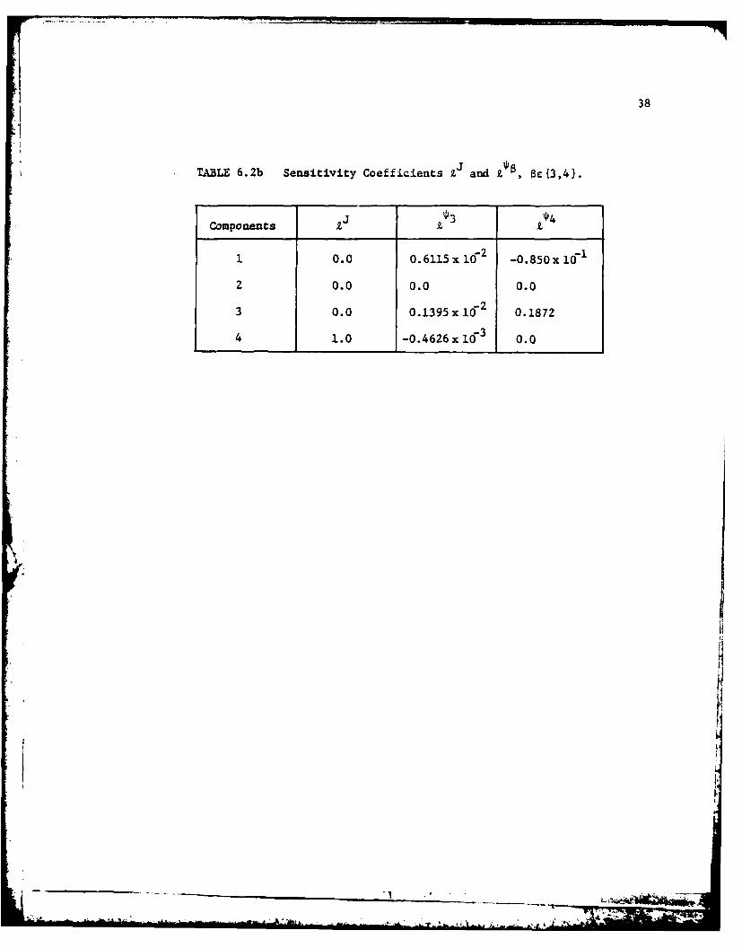
To study the numerical results of design sensitivity analysis, the

sensitivity coefficients t 8W(1,2,3,4), and 1 0 were first calculated

.. .

31

for the 2 second interval, with initial estimates of the design parameters

given in Table 6.2a. Lower and upper bounds on the first three design

parameters were selected as bL = [0.8, 0.2, 5.0]T and bU = [1.5, 0.8, 16.0].12

Also A 2(max) = 10.0 and *2 (max) = 0.3.22

The cost and constraint functional were evaluated for 0.1% and 1.0%

perturbations of the first, second, and fourth design parameters and 0.01%

and 0.1% changes in the third design parameter. The corresponding changes

in the functionals given in Table 6.2a are presented in compact form. In

these computations the integrands of *1 ' W29 and 13 have been normalized

12 12 2by dividing by A2 (max), X2 (max), and b4 , respectively. Sensitivity

coefficients are given in Table 6.2b.

The predicted changes S = £Za6b in the cost and constraint functions

due to the foregoing design perturbations were calculated and are given

in Table 6.2a. It is observed from the table that terms of the form Z 6b

match satisfactorily with the actual changes in *', 8 =0,3,4. The slight

discrepancies are attributed to various approximations and linearizations

at many steps of both transient and sensitivity analysis and the coarse

time grid used for numerical integration.

In carrying out the optimal design algorithm for the two second

interval, a design reduction ratio of 3 percent was used to compute the

0step size in the first iteration. The initial estimate b and design

variable bounds are given in Table 6.3.

At the starting design 116b11 = 0.1248 and 116b 2 11 -i 0.2307. Con-

straints 3 and 4 are violated and the lower bound constraint on design

parameter b3 is tight. After 6 iterations, as the algorithm approached

3'

~..** ... r

-, '4

32

the optimum design, I 1b 1 reduced to 0.8404 x 10- 5 , 1ib21 1 reduced to

0.2669 x 10- , and design variable constraints on bI, b2 and b became2 3

tight. The optimum design is given in Table 6.3.

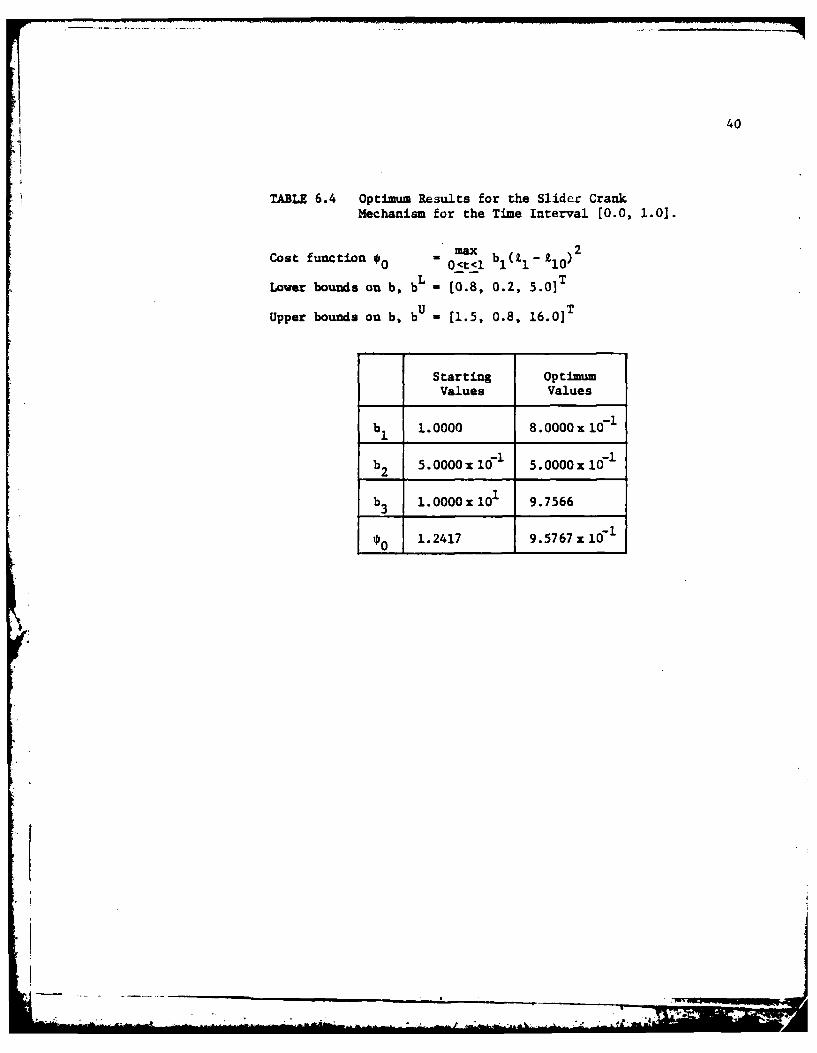
Next, the design problem is considered for the interval [0,1],

with design and initial data given in Table 6.4. For this case a design

reduction ratio .of 10% was used in computing the step size in the first

iteration. At the starting design J1lbl1l - 0.0, I16b 2 1, - 0.1106 x 10-2 ,

and constraint 3 is violated. In the second iteration l16b'1I = 0.7348,

16b 211 - 3.814 x 10- , and again constraint 3 is violated. After 18

iterations, as the algorithm approaches the optimum design, 116blI-

5.567 x 10- 3, lib21 - 3.018 x 10-3 , and design parameter constraints on

b and b2 are tight. The optimum design is given in Table 6.4.

1 2

V(

I,<aa

33

References

1. Chua, L. 0. and Lin, P-M., Computer Aided Analysis of Electronic

Circuits, Prentice-Hall, Englewood Cliffs, New Jersey, 1975.

2. Zienkiewicz, D. C., The Finite Element Method, Third Edition,

McGraw-Hill, New York, 1977.

3. Paul, B., "Analytical Dynamics of Mechanisms - A Computer Oriented

Overview", Mechanism and Machine Theory, Vol. 10, 1975, pp. 481-507.

4. Sheth, P. N., "A Digital Computer Based Simulation Procedure for

Multiple Degree of Freedom Mechanical Systems with Geometric

Contraints," Ph.D. Thesis, University of Wisconsin, Madison, Wisconsin,

1972.

5. Chace, M. A. and Smith, D. A., "DAMN - Digital Computer Program for

the Dynamic Analysis of Generalized Mechanical Systems", SAE Trans-

actions, Vol. 80, 1971, pp. 969-987.

6. Orlandea, N., Node-Analogous, Sparsity Oriented Methods for Simula-

tion of Mechanical Dynamic Systems," Ph.D. Thesis, University of

Michigan, Ann Arbor, Michigan, 1973.

7. Greenwood, D. T., Principles of Dynamics, Prentice-Hall, Englewood

Cliffs, New Jersey, 1965.

8. Brameller, A., Allen, R. N., and Haman, Y. M., Sparsity, Pitman

Publishing Corp., New York, 1976.

9. Barman, N. C., Sensitivity Analysis and Optimization of Constrained

Mechanical System Dynamics, Ph.D. Thesis, Materials Division,

University of Iowa, 1978.

34

10. Haug, E.J., and Arora, J.S., "Design Sensitivity Analysis of Elastic

Mechanical Systems", Computer Methods in Applied Mechanics and

Engineering, Vol. , 1978, pp.

11. Haug, E.J., and Arora, J.S. Applied Optimal Design, John Wiley,

New York, 1979, (to appear).

I.I

- A ...-.'

35

TABLE 6.1 Initial Estimates of the Parameters for the Slider-Crank Mechanism (Units in Inch, Pound-Force, SecondSystem).

LINK DESCRIPTION

m. =M(1) =1. m 2 =M(2) =4. % =M(3) =1. m4 =M(4) =3.

Jl =JIN(1) =1. J2 =JIN(2) =10. J3 =J1N(3) =4. J4 =JIN(4) =2.

xI =X(1) =0. x2 =X(2) =1. x3 =X(3) =8.667 x4 =X(4) =17.32

Yl =Y(1) =0. y2 =Y(2) =0. Y3 =Y(3) =5.25 Y4 =Y(4) =.5

I =PHI(l) =0. #2 =PHI(2) =1.5708 3 =PHI(3) =-.5236 04 =PHI(4) =0.

* Qxl =FX(1) =0. Qx2 =FX(2) =0. Qx3 =FX(3) =0. Qx4 =FX(4) =0.

* QYl =FY(1) =0. QY2 =FY(2) =0. QY3 =FY(3) =0. Qy4=FY(4) =0.

* %1 =TQ(1) =0. Q 2 =TQ(2) =100. Q 3 =TQ(3) =0. QO4=TQ(4) =0.

JOINT DESCRIPTION

i =IB(1,1) =1 i =IB(1,2)=2 i =IB(1,3)=3 i =IB(1,4) =4

12 =Xl(1) =0. 23 =Xl(2) =9.0 34 =XI(3) =10. &4 1 =XI(4) =0.

912 =YI(1) =0. n23 =Yl(2) =0. 114 =YI(3) =0. n41 =Yl(4) =0.5

j =IB(2,1) =2 j =IB(2,2)=3 j =IB(2,3)=4 j =IB(2,4) =1

21 =X2(1) =-i. 32 =X2(2) =-10. 43 =X2(3) =0. &14 =X2(4) =0.

121 =Y2(1) =0. T132 =Y2(2) =0. r43 =Y2(3) =0. n 4 =Y2(4) 1.0

SPRING-DAMPER DESCRIPTION

i =IBSD(1,1)=1 C S4=XF1(1) =35. nS14=YF1(1) =0.5 j =IBSD(2,1)=4

5s4 1=XF2(1) =2. n s41=YF2(1) =0. k14 =SK(1) =1. C14 =DC(1) =1.

.14 =SDL(1) =15.68 0 14=SDLO(1)=15.68 F0 4 =SDF(1) =0.

* The parameters FX, FY, and TQ represent components of force and moment

that are reduced to the centers of mass on each link and contribute to

Qxi' QYi' and Q0i in Eq. 2.4.

II

36

LM Ln LM Ln -4 L n L

61,

4

w 10

IT'

-4

-4 14-

ImI

--4

CN 4

0n 0 i

37

o- C14 0

4C) CD

0T 0I a% 0 T 0 0

-7 - f - IT en en IT-?14 - 4 .4 - 0 r-f --T -4

-IT -. ~ ~ - r- -T IT -7 -

Cl C C l l C Cl C4C

o CD0 * 0 0 0: 0

0 0 -4 r-4 -4 -4'0 --1 )x x x x

x. 0 x -T Lf) C0 LIN I-en ul .o -4 aN0 -T

- 0 aC0 % 0D -4 0 Cl) %D0 cn 0D 'o -4 0

ol 1- 0 0

0n 0 0n M0 0-4 n m r4 -4

o 0 0 - 0 IT -4 -u 0 CD0 00 0

0l 4 cn cn c n m cn n e

'.01 0 0 0 10 0 0 10 10 10-4 -4 -4 -4 -4 -.4 -4 -4 -4x x x x x x 4 '4 x

14 ~-1 -4 1- en~ -T7 I Lc~ 0 '.0 0 4 r cn 0 00 C

-9 %. 0 '0 r, 0 L, '.D r, 00%. - '0 '.0 %D -4 %D0 r- 1-1

a4 Clr-

o 0 0 0 0D 0 0 0- 0

-44

I I,

'0 0D 0D 0 0D 0D 0D 0 0

C; C

- 0D 0D C0 CD C 0 0 0 D 0

4 I4

0 0i

38

TABLE 6.2b Sensitivity Coefficients 2X and Z Be{3,4}.

Components 2. 3 24

-2-.1 0.0 0.6115 x 10 -0.850 x 10

2 0.0 0.0 0.0

0.0 -23 0.0 0.1395 x 10 0.1872

4 1.0 -0.4626 x 10 3 0.0

39

TABLE 6.3 Optimum Results for the Slider Crank Mechanismfor the Time Interval [0.0, 2.0].

Cost function m b ( - t ) 20 O<t<2 1 1 1

Lower bounds on b, bL = 10.8, 0.2, 9.0] T

Upper bounds on b, b = 1.5, 0.8, 12.01T

Starting OptimumValues Values

b 1 8.2440 x 1071 8.0000 x i0 - I

b2 5. 0000 x 10 1 5.0000 x 10 -

b3 9.0000 9.0000

* l0 1.1159 x 10 1.00115 x 101

ism

40

TABLE 6.4 Optimum Results for the Slider CrankMechanism for the Time Interval (0.0, 1.0].

Cost function i0 0<xb( - I ) 2

Lower bounds on b, bL . [0.8, 0.2, 5.0] T

Upper bounds on b, bU = (1.5, 0.8, 16.0] T

Starting OptimumValues Values

b 1.0000 8.0000 x 1071

1 ~ -__ _ __1__ _

b2 5.0000 x 10 5.0000x 10

b3 1.0000 x 101 9.7566

*0 1.2417 9.5767 x 10- 1

41

p

/7-f -0

Figure 2.1 Definition of the Generalized Co-ordinateof the i-th Body.

* 42

rji

Figure 2.2 Joint Co-ordinates

43

line of relativex motion between bodies

Figure 2.3 Translational Joint

rji.

Ri.j

44

TsqI

/ j x

Fiur .4C~odflt frth SrflDPe omiato

- - .

45

cn

0:En 4),F-4P4 0

4V4

.0 Cii

00

U~tjU

I

46

40

N5

-4

C

*0

4-4 Cu

9-4

-4Cu

'a-I

-44.1-4w

*3

____________ C',

U-'

*3

00S.''-I

( ri____1~I

r

I Read initial estimates, bounds, number of constraints, 47and other parameters related to the design problem.

Initialize system parameters for implementation ofthe DYNANL program.

(INDATA)

Relate design parameters with system parameters.(RELATE)

Obtain the solution of the equations of motionand store the results on disk.

(DYNANL)

Evaluate integrands of cost and constraint functions.(HALS)

Solve adjoint equations and find the sensitivitymatrices for the violated functional constraints.

(ADJONT, AHLPS I)

Test the design parameter constraints and find thesensitivity matrices.

(DPARMC)

Find the sensitivity vector.(AHLPSI)

Compute N* and the Lagrange Multipliers, check theirsigns, and compute design improvements.(NEWB) I

Test the convergence criteria.

Figure 5.3 Flow Diagram of the DADS Computer Program.

-I 48

rn -4

cu

.0 C0

CC.)

C~Cu

C~Cu

>1-4

_%ALA

1 49

t I '

45

C ae ~E C .r -9 F DFPR

C 0D AE (3

, 3 U 7

.Z P . TV 8 ... --

N K0 L

S..0 A .9 K 8R 3 AL 0

* S21Z 08MN CEW T

'C U - * .Y V56 90

78 ABS K L

.T J N.w x 1 2

YZ 34GHI COEj FCPQ RST U

vwX..Y2 3 .6 60.

ZI 45 79 A

Figure 6.2 Symbolic Listing of the Nonzero Entries in the Jacobian

Matrix for the Example Slider-Crank Mechanism

DISTRIBUTION LIST

Please notify USATACOM, DRSTA-ZSA, Warren, Michigan 48090, of correctionsand/or changes in address.

Commander (25) Director (01)US Army Tk-Autmv Command Defense Advanced ResearchR&D Center Projects AgencyWarren, MI 48090 1400 Wilson Boulevard

Arlington, VA 22209Superintendent (02)US Military Academy Commander (01)ATTN: Dept of Engineering US Army Combined Arms Combat

Course Director for Developments ActivityAutomotive Engineering ATTN: ATCA-CCC-S

Fort Leavenworth, KA 66027Commander (01)US Army Logistic Center Commander (01)Fort Lee, VA 23801 US Army Mobility Equipment

Research and Development CommandUS Army Research Office (02) ATTN: DRDME-RTP.O. Box 12211 Fort Belvoir, VA 22060ATTN: Dr. F. Schmiedeshoff

Dr. R. Singleton Director (02)Research Triangle Park, NC 27709 US Army Corps of Engineers

Waterways Experiment StationHQ, DA (01) P.O. Box 631ATTN: DAMA-AR Vicksburg, MS 39180

Dr. HerschnerWashington, D.C. 20310 Commander (01)

US Army Materials and Mechanics

HQ, DA (01) Research CenterOffice of Dep Chief of Staff ATTN: Mr. Adachifor Rsch, Dev G Acquisition Watertown, MA 02172ATTN: DAMA-AR

Dr. Charles Church Director (03)Washington, D.C. 20310 US Army Corps of Engineers

Waterways Experiment Station

HQ, DARCOM P.O. Box 6315001 Eisenhower Ave. ATTN: Mr. NuttallATTN: DRCDE Vicksburg, MS 39180

Dr. R.L. HaleyAlexandria, VA 22333 Director (04)

US Army Cold Regions Research& Engineering LabP.O. Box 282ATTN: Dr. Freitag, Dr. W. HarrisonDr. Liston, LibraryHanover, NH 03755

President (02) Director (02)Army Armor and Engineer Board Defense Documentation CenterFort Knox, KY 40121 Cameron Station

Alexandria, VA 22314Commander (01)US Army Arctic Test Center US Marine Corps (01)APO 409 Mobility & Logistics DivisionSeattle, WA 98733 Development and Ed Command

ATTN: Mr. HicksonCommander (02) Quantico, VA 22134US Army Test & EvaluationCommand Keweenaw Field Station (01)ATTN: AMSTE-BB and AMSTE-TA Keweenaw Research CenterAberdeen Proving Ground, MD Rural Route 121005 P.O. Box 94-D

ATTN: Dr. Sung M. LeeCommander (01) Calumet, MI 49913US Army Armament Researchand Development Command Naval Ship Research & (02)ATTN: Mr. Rubin Dev CenterDover, NJ 07801 Aviation & Surface Effects Dept

Code 161Commander (01) Washington, D.C. 20034US Army Yuma Proving GroundATTU: STEYP-RPT Director (01)Yuma, AZ 85364 National Tillage Machinery Lab

Box 792Commander (01) Auburn, AL 36830US Army Natic LaboratoriesATTN: Technical Library Director (02)Natick, MA 01760 USDA Forest Service Equipment

Development CenterDirector (01) 444 East Bonita AvenueUS Army Human Engineering Lab San Dimes, CA 91773ATTN: Mr. EckelsAberdeen Proving Ground, MD Engineering Societies (01)21005 Library

345 East 47th StreetDirector (02) New York, NY 10017US Army Ballistic Research LabAberdeen Proving Ground, MD Dr. I.R. Erlich (01)21005 Dean for Research

Stevens Institute of TechnologyDirector (02) Castle Point StationUS Army Materiel Systems Hoboken, NJ 07030Analysis AgencyATTN: AMXSY-CMAberdeen Proving Ground, MD21005

t4

Grumman Aerospace Corp (02) CALSPAN Corporation (01)South Oyster Bay Road Box 235ATTN: Dr. L. Karafiath Library

Mr. F. Markow 4455 Benesse StreetM/S A08/35 Buffalo, NY 14221

Bethpage, NY 11714SEM, (01)

Dr. Bruce Liljedahl (01) ForsvaretsforskningsanstaltAgricultural Engineering Dept Avd 2Purdue University Stockholm 80, SwedenLafayette, IN 46207

Mr. Hedwig (02)Mr. H.C. Hodges (01) RU 111/6Nevada Automotive Test Center Ministry of DefenseBox 234 5300 Bonn, GermanyCarson City, NV 89701

Foreign Science & Tech (01)Mr. R.S. Wismer (01) CenterDeere & Company 220 7th Street North EastEngineering Research ATTN: AMXST-GEI3300 River Drive Mr. Tim NixMoline, IL 61265 Charlottesville, VA 22901

Oregon State University (01) General Research Corp (01)Library 7655 Old Springhouse RoadCorvallis, OR 97331 Westgate Research Park

ATTN: Mr. A. ViiluSouthwest Research Inst (01) McLean, VA 221018500 Culebra RoadSan Antonia, TX 78228 Commander (01)

US Army Developmant andFMC Corporation (01) Readiness CommandTechnical Library 5001 Eisenhower AvenueP.O. Box L201 ATTN: Dr. R.S. WisemanSan Jose, CA 95108 Alexandria, VA 22333

Mr. J. Appelblatt (01)Director of EngineeringCadillac Gauge CompanyP.O. Box 1027Warren, MI 48090

Chrysler Corporation (02)Mobility Research Laboratory,Defense EngineeringDepartment 6100P.O. Box 751Detroit, MI 48231