I. Portable, Extensible Toolkit for Scientific Computation

Boyana Norris (representing the PETSc team)

Mathematics and Computer Science Division

Argonne National Laboratory, USA March, 2009

1

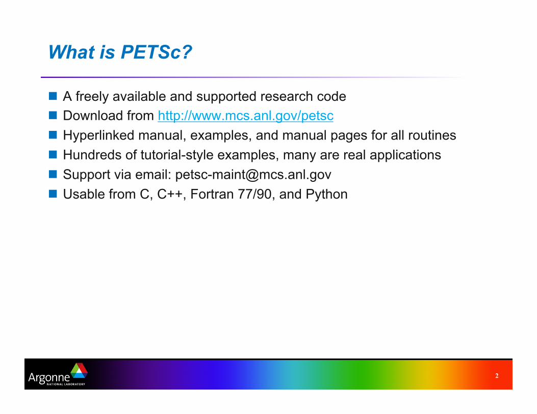
What is PETSc?

  A freely available and supported research code   Download from http://www.mcs.anl.gov/petsc   Hyperlinked manual, examples, and manual pages for all routines   Hundreds of tutorial-style examples, many are real applications   Support via email: petsc-maint@mcs.anl.gov   Usable from C, C++, Fortran 77/90, and Python

2

What is PETSc?

 Portable to any parallel system supporting MPI, including:

–  Tightly coupled systems •  Blue Gene/P, Cray XT4, Cray T3E, SGI Origin, IBM SP, HP 9000, Sub Enterprise

–  Loosely coupled systems, such as networks of workstations •  Compaq,HP, IBM, SGI, Sun, PCs running Linux or Windows, Mac OS X

 PETSc History –  Begun September 1991 –  Over 20,000 downloads since 1995 (version 2), currently 300 per

month

 PETSc Funding and Support –  Department of Energy

•  SciDAC, MICS Program, INL Reactor Program –  National Science Foundation

•  CIG, CISE, Multidisciplinary Challenge Program

3

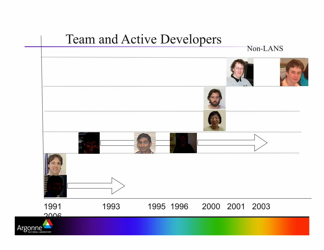
1991 1993 1995 1996 2000 2001 2003 2006

Non-LANS Team and Active Developers

How did PETSc Originate?

PETSc was developed as a Platform for Experimentation.

We want to experiment with different •  Models •  Discretizations •  Solvers •  Algorithms (which blur these boundaries)

Successfully Transitioned from Basic Research to Common Community Tool   Applications of PETSc

–  Nano-simulations (20) –  Biology/Medical(28) –  Cardiology –  Imaging and Surgery –  Fusion (10) –  Geosciences (20) –  Environmental/Subsurface Flow (26) –  Computational Fluid Dynamics (49) –  Wave propagation and the Helmholz equation (12) –  Optimization (7) –  Other Application Areas (68) –  Software packages that use or interface to PETSc (30) –  Software engineering (30) –  Algorithm analysis and design (48)

6

Who Uses PETSc?

  Computational Scientists –  PyLith (TECTON), Underworld, Columbia group

  Algorithm Developers –  Iterative methods and Preconditioning researchers

  Package Developers –  SIPs, SLEPc, TAO, MagPar, StGermain, Dealll

7

The Role of PETSc

Developing parallel, nontrivial PDE solvers that deliver high performance is still difficult and requires months (or even years) of concentrated effort.

PETSc is a tool that can ease these difficulties and reduce the development time, but it is not a black-box PDE solver, nor a silver bullet.

8

Features

 Many (parallel) vector/array operations   Numerous (parallel) matrix formats and operations   Numerous linear solvers   Nonlinear solvers   Limited ODE integrators   Limited parallel grid/data management   Common interface for most DOE solver software

9

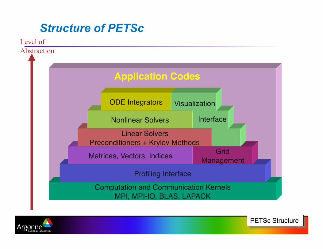
Structure of PETSc

10

Computation and Communication Kernels MPI, MPI-IO, BLAS, LAPACK

Profiling Interface

Application Codes

Matrices, Vectors, Indices Grid Management

Linear Solvers Preconditioners + Krylov Methods

Nonlinear Solvers

ODE Integrators Visualization

Interface

PETSc Structure

Level of Abstraction

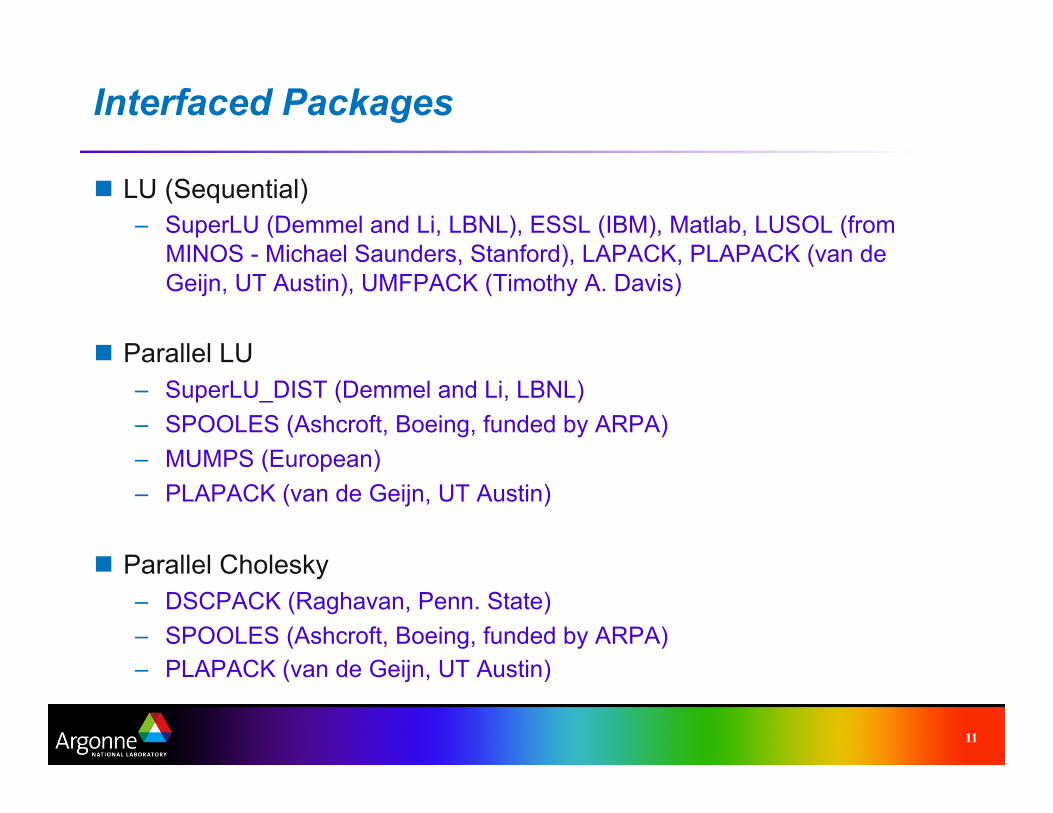
Interfaced Packages

  LU (Sequential) –  SuperLU (Demmel and Li, LBNL), ESSL (IBM), Matlab, LUSOL (from

MINOS - Michael Saunders, Stanford), LAPACK, PLAPACK (van de Geijn, UT Austin), UMFPACK (Timothy A. Davis)

  Parallel LU –  SuperLU_DIST (Demmel and Li, LBNL) –  SPOOLES (Ashcroft, Boeing, funded by ARPA) –  MUMPS (European) –  PLAPACK (van de Geijn, UT Austin)

  Parallel Cholesky –  DSCPACK (Raghavan, Penn. State) –  SPOOLES (Ashcroft, Boeing, funded by ARPA) –  PLAPACK (van de Geijn, UT Austin)

11

Interfaced Packages

  XYTlib – parallel direct solver (Fischer and Tufo, ANL)   SPAI – Sparse approximate inverse (parallel)

–  Parasails (Chow, part of Hypre, LLNL) –  SPAI 3.0 (Grote/Barnard)

  Algebraic multigrid –  Parallel BoomerAMG (part of Hypre, LLNL) –  ML (part of Trilinos, SNL)

  Parallel ICC(0) – BlockSolve95 (Jones and Plassman, ANL)   Parallel ILU

–  BlockSolve95 (Jones and Plassman, ANL) –  PILUT (part of Hypre, LLNL) –  EUCLID (Hysom – also part of Hypre, ODU/LLNL)

  Sequential ILUDT (SPARSEKIT2- Y. Saad, U of MN)

12

Interfaced Packages

  Parititioning –  Parmetis –  Chaco –  Jostle –  Party –  Scotch

 ODE integrators –  Sundials (LLNL)

  Eigenvalue solvers –  BLOPEX (developed by Andrew Knyazev)

  FFTW   SPRN

13

Child Packages of PETSc

  SIPs - Shift-and-Invert Parallel Spectral Transformations   SLEPc - scalable eigenvalue/eigenvector solver packages.   TAO - scalable optimization algorithms   veltisto (“optimum”)- for problems with constraints which are time-

independent PDEs.

  All have PETSc’s style of programming

14

What Can We Handle?

  PETSc has run problem with 500 million unknowns –  http://www.scconference.org/sc2004/schedule/pdfs/pap111.pdf

  PETSc has run on over 6,000 processors efficiently –  ftp://info.mcs.anl.gov/pub/tech_reports/reports/P776.ps.Z

  PETSc applications have run at 2 Teraflops –  LANL PFLOTRAN code

  PETSc also runs on your laptop

  Only a handful of our users ever go over 64 processors

15

Modeling of Nanostructured Materials

16

*

System

size

Accuracy

Example 1:

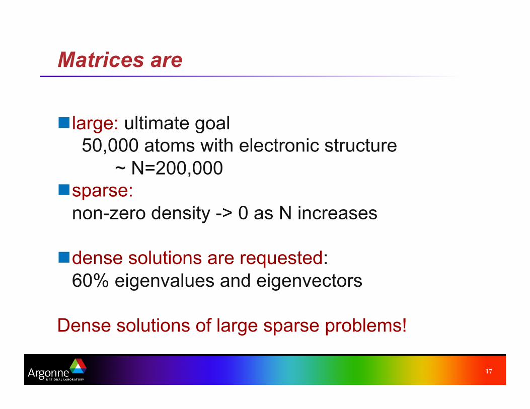
Matrices are

 large: ultimate goal 50,000 atoms with electronic structure ~ N=200,000

 sparse: non-zero density -> 0 as N increases

 dense solutions are requested: 60% eigenvalues and eigenvectors

Dense solutions of large sparse problems!

17

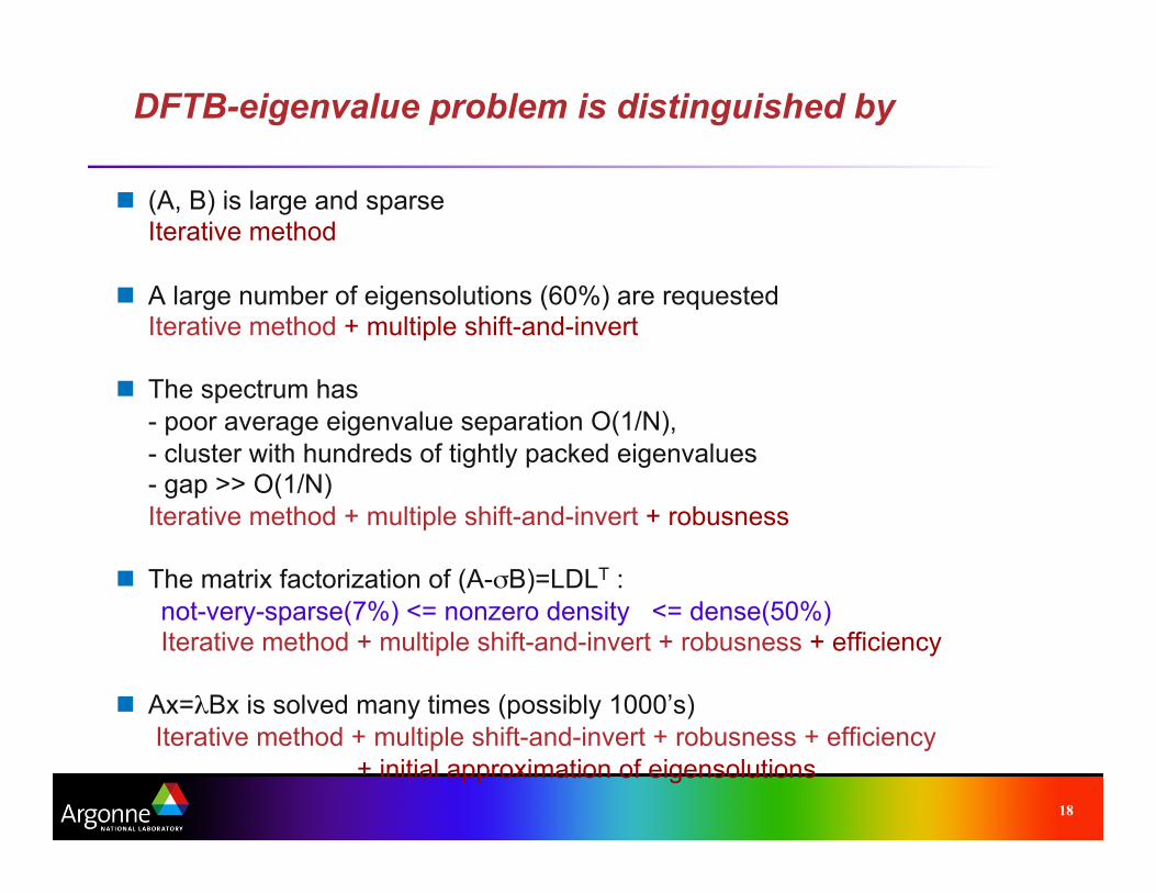
DFTB-eigenvalue problem is distinguished by

  (A, B) is large and sparse Iterative method

  A large number of eigensolutions (60%) are requested Iterative method + multiple shift-and-invert

  The spectrum has - poor average eigenvalue separation O(1/N), - cluster with hundreds of tightly packed eigenvalues - gap >> O(1/N) Iterative method + multiple shift-and-invert + robusness

  The matrix factorization of (A-σB)=LDLT : not-very-sparse(7%) <= nonzero density <= dense(50%) Iterative method + multiple shift-and-invert + robusness + efficiency

  Ax=λBx is solved many times (possibly 1000’s) Iterative method + multiple shift-and-invert + robusness + efficiency

+ initial approximation of eigensolutions 18

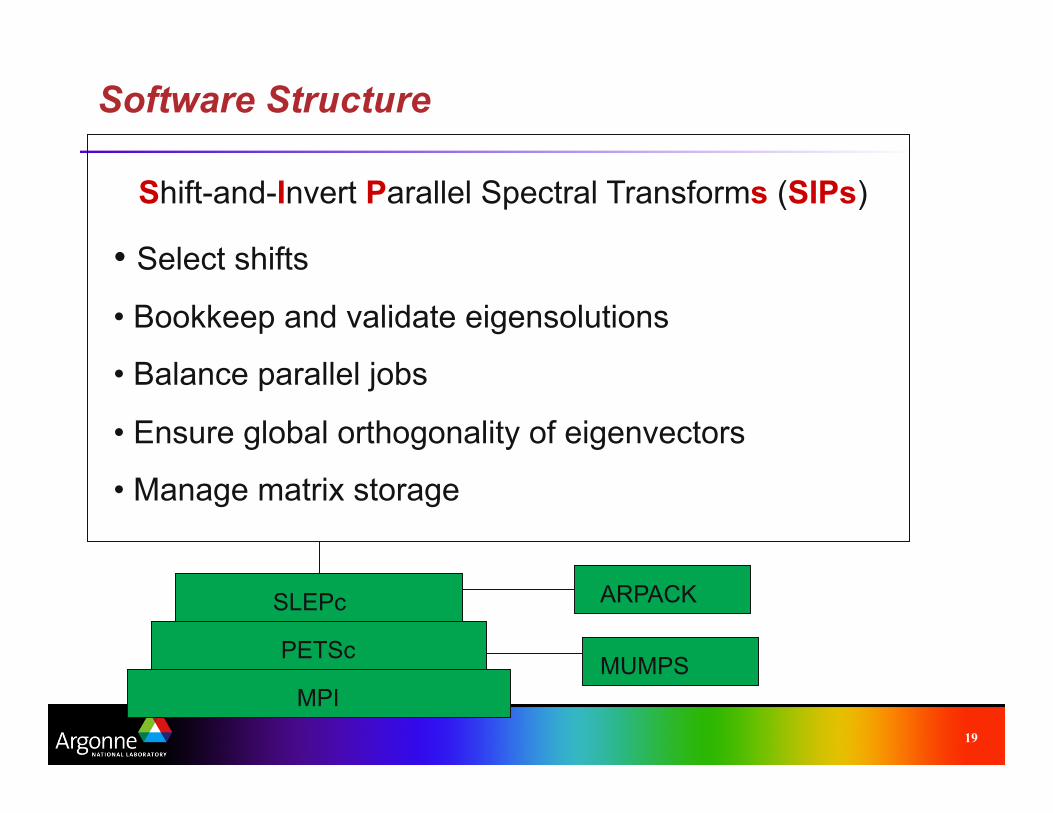
Software Structure

19

MPI

PETSc

SLEPc

MUMPS

ARPACK

Shift-and-Invert Parallel Spectral Transforms (SIPs)

•  Select shifts

•  Bookkeep and validate eigensolutions

•  Balance parallel jobs

•  Ensure global orthogonality of eigenvectors

•  Manage matrix storage

FACETS: Framework Application for Core-Edge Transport Simulations

  https://facets.txcorp.com/facets   PI: John Cary, Tech-X Corporation

 Goal: Providing modeling of a fusion device from the core to the wall

  TOPS Emphasis in FACETS

–  Incorporate TOPS expertise in scalable nonlinear algebraic solvers into the base physics codes that provide the foundation for the coupled models

–  Study mathematical challenges that arise in coupled core-edge and transport-turbulence systems

20

IU NYU

Lodestar

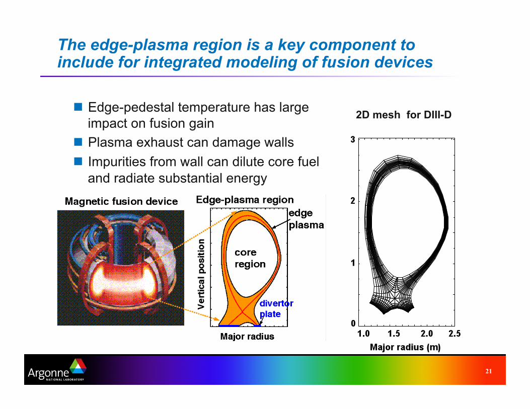
The edge-plasma region is a key component to include for integrated modeling of fusion devices

  Edge-pedestal temperature has large impact on fusion gain

  Plasma exhaust can damage walls   Impurities from wall can dilute core fuel

and radiate substantial energy

21

2D mesh for DIII-D

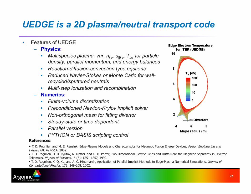
UEDGE is a 2D plasma/neutral transport code

•  Features of UEDGE –  Physics: •  Multispecies plasma; var. ni,e, u||i,e, Ti,e for particle

density, parallel momentum, and energy balances •  Reaction-diffusion-convection type eqstions •  Reduced Navier-Stokes or Monte Carlo for wall-

recycled/sputtered neutrals •  Multi-step ionization and recombination

–  Numerics: •  Finite-volume discretization •  Preconditioned Newton-Krylov implicit solver •  Non-orthogonal mesh for fitting divertor •  Steady-state or time dependent •  Parallel version •  PYTHON or BASIS scripting control

22

•  T. D. Rognlien and M. E. Rensink, Edge-Plasma Models and Characteristics for Magnetic Fusion Energy Devices, Fusion Engineering and Design, 60: 497-514, 2002. •  T. D. Rognlien, D. D. Ryutov, N. Mattor, and G. D. Porter, Two-Dimensional Electric Fields and Drifts Near the Magnetic Separatrix in Divertor Tokamaks, Physics of Plasmas, 6 (5): 1851-1857, 1999. •  T. D. Rognlien, X. Q. Xu, and A. C. Hindmarsh, Application of Parallel Implicit Methods to Edge-Plasma Numerical Simulations, Journal of Computational Physics, 175: 249-268, 2002.

References:

Outline

 Overview of PETSc –  Linear solver interface: KSP –  Nonlinear solver interface: SNES –  Profiling and debugging

 Ongoing research and developments

23

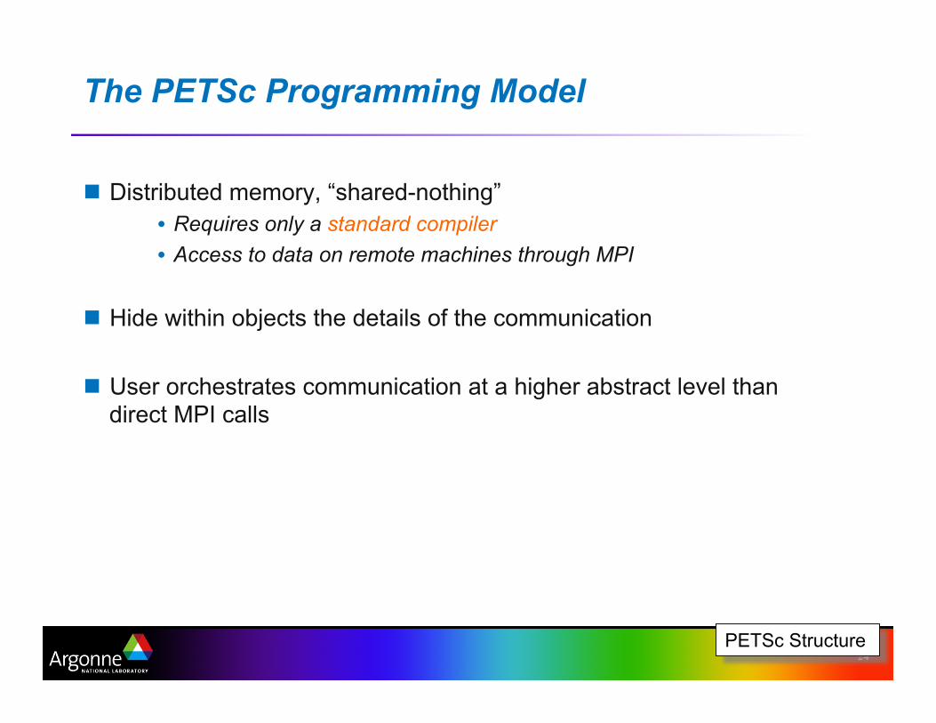
The PETSc Programming Model

  Distributed memory, “shared-nothing” •  Requires only a standard compiler •  Access to data on remote machines through MPI

  Hide within objects the details of the communication

  User orchestrates communication at a higher abstract level than direct MPI calls

24 PETSc Structure

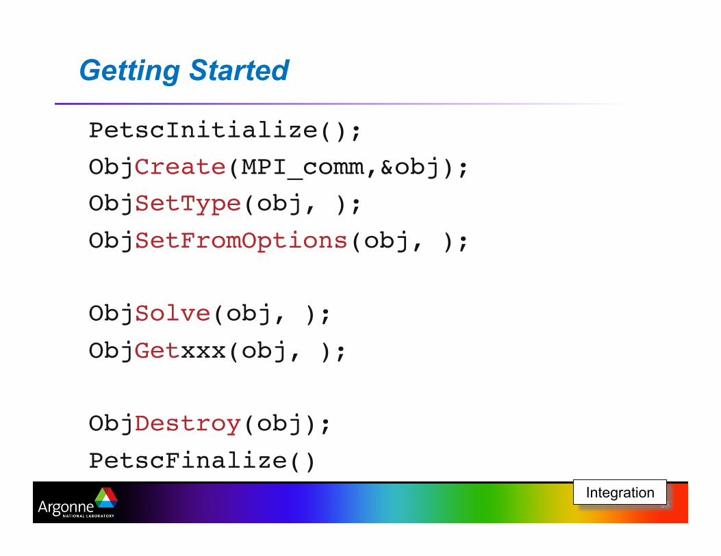
Getting Started

PetscInitialize(); ObjCreate(MPI_comm,&obj); ObjSetType(obj, ); ObjSetFromOptions(obj, );

ObjSolve(obj, ); ObjGetxxx(obj, );

ObjDestroy(obj); PetscFinalize()

25 Integration

PETSc Numerical Components

26

Compressed Sparse Row

(AIJ)

Blocked Compressed Sparse Row

(BAIJ)

Block Diagonal (BDIAG)

Dense Other

Indices Block Indices Stride Other Index Sets (IS)

Vectors (Vec)

Line Search Trust Region

Newton-based Methods Other

Nonlinear Solvers (SNES)

Additive Schwartz

Block Jacobi Jacobi ILU ICC LU

(Sequential only) Others

Preconditioners (PC)

Euler Backward Euler

Pseudo Time Stepping Other

Time Steppers (TS)

GMRES CG CGS Bi-CG-STAB TFQMR Richardson Chebychev Other

Krylov Subspace Methods (KSP)

Matrices (Mat)

Distributed Arrays(DA)

Matrix-free

Linear Solver Interface: KSP

27

PETSc

Application Initialization Evaluation of A and b Post-

Processing

Solve Ax = b PC

Linear Solvers (KSP)

PETSc code User code

Main Routine

solvers:linear beginner

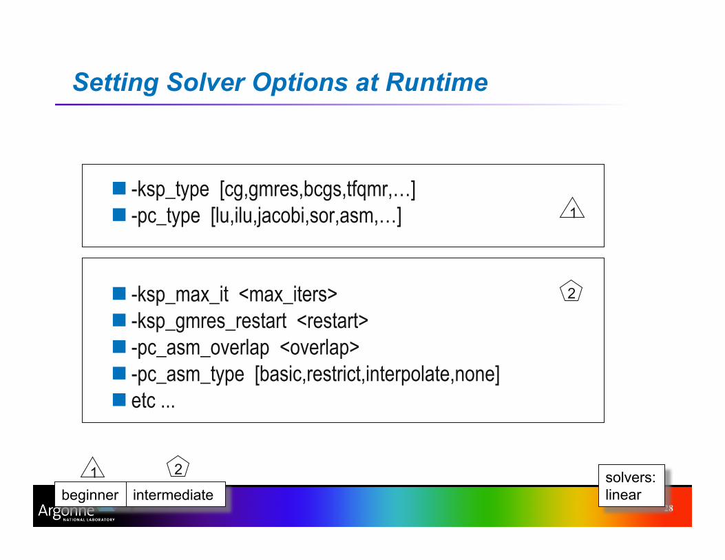
Setting Solver Options at Runtime

 -ksp_type [cg,gmres,bcgs,tfqmr,…]  -pc_type [lu,ilu,jacobi,sor,asm,…]

 -ksp_max_it <max_iters>  -ksp_gmres_restart <restart>  -pc_asm_overlap <overlap>  -pc_asm_type [basic,restrict,interpolate,none]  etc ...

28

solvers:linear beginner

1 intermediate

2

1

2

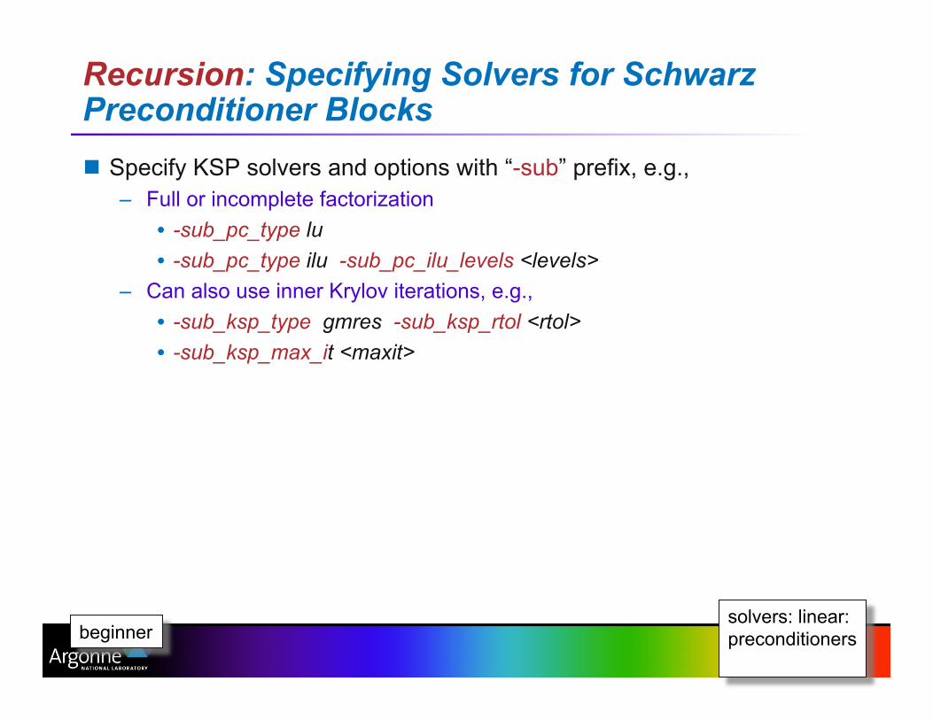
Recursion: Specifying Solvers for Schwarz Preconditioner Blocks   Specify KSP solvers and options with “-sub” prefix, e.g.,

–  Full or incomplete factorization •  -sub_pc_type lu •  -sub_pc_type ilu -sub_pc_ilu_levels <levels>

–  Can also use inner Krylov iterations, e.g., •  -sub_ksp_type gmres -sub_ksp_rtol <rtol> •  -sub_ksp_max_it <maxit>

29

solvers: linear: preconditioners beginner

Flow of Control for PDE Solution

30

PETSc code User code

Application Initialization

Function Evaluation

Jacobian Evaluation

Post- Processing

PC PETSc

Main Routine

Linear Solvers (KSP)

Nonlinear Solvers (SNES)

Timestepping Solvers (TS)

PETSc Structure

Example (UEDGE): Solve F(u) = 0

31

Post- Processing

Application Initialization Function

Evaluation

Jacobian Evaluation

PETSc

Nonlinear Solvers (SNES)

PETSc code

Application code

UEDGE finite differencing Jacobian for preconditioning matrix; PETSc code for matrix-free Jacobian-vector products

Matrices Vectors

Krylov Solvers Preconditioners

GMRES

TFQMR

BCGS

CGS

BCG

Others…

ASM

ILU

B-Jacobi

SSOR

Multigrid

Others…

AIJ

B-AIJ

Diagonal

Dense

Matrix-free

Others…

Sequential

Parallel

Others…

UEDGE Driver + Timestepping

Algorithms and data structures originally employed by UEDGE

Nonlinear Solver Interface: SNES

Goal: For problems arising from PDEs, support the general solution of F(u) = 0

User provides: –  Code to evaluate F(u) –  Code to evaluate Jacobian of F(u) (optional)

•  or use sparse finite difference approximation •  or use automatic differentiation –  AD support via collaboration with P. Hovland and B. Norris –  Coming in next PETSc release via automated interface to

ADIFOR and ADIC (see http://www.mcs.anl.gov/autodiff)

32

solvers: nonlinear

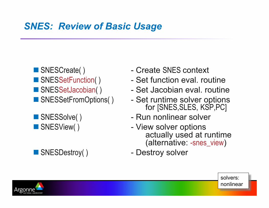
SNES: Review of Basic Usage

 SNESCreate( ) - Create SNES context  SNESSetFunction( ) - Set function eval. routine  SNESSetJacobian( ) - Set Jacobian eval. routine  SNESSetFromOptions( ) - Set runtime solver options

for [SNES,SLES, KSP,PC]  SNESSolve( ) - Run nonlinear solver  SNESView( ) - View solver options

actually used at runtime (alternative: -snes_view)

 SNESDestroy( ) - Destroy solver

33

solvers: nonlinear

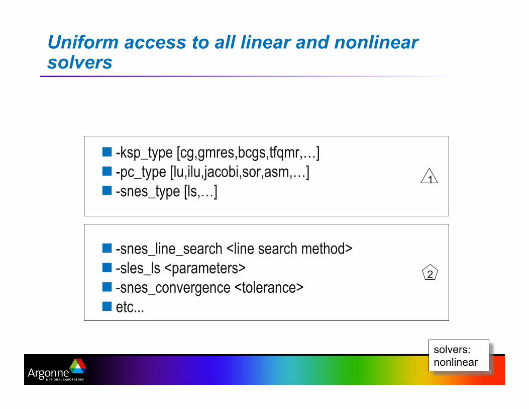
Uniform access to all linear and nonlinear solvers

 -ksp_type [cg,gmres,bcgs,tfqmr,…]  -pc_type [lu,ilu,jacobi,sor,asm,…]  -snes_type [ls,…]

 -snes_line_search <line search method>  -sles_ls <parameters>  -snes_convergence <tolerance>  etc...

34

solvers: nonlinear

1

2

PETSc Programming Aids

  Correctness Debugging –  Automatic generation of tracebacks –  Detecting memory corruption and leaks –  Optional user-defined error handlers

  Performance Profiling –  Integrated profiling using -log_summary –  Profiling by stages of an application –  User-defined events

35 Integration

Ongoing Research and Developments

  Framework for unstructured meshes and functions defined over them

  Framework for multi-model algebraic system

  Bypassing the sparse matrix memory bandwidth bottleneck –  Large number of processors (nproc =1k, 10k,…) –  Peta-scale performance

  Parallel Fast Poisson Solver

 More TS methods  …

36

Framework for Meshes and Functions Defined over Them

 The PETSc DA class is a topology and discretization interface. –  Structured grid interface

• Fixed simple topology –  Supports stencils, communication, reordering

•  Limited idea of operators

 The PETSc Mesh class is a topology interface –  Unstructured grid interface

• Arbitrary topology and element shape –  Supports partitioning, distribution, and global orders

37

 The PETSc DM class is a hierarchy interface. –  Supports multigrid

• DMMG combines it with the MG preconditioner

–  Abstracts the logic of multilevel methods

 The PETSc Section class is a function interface –  Functions over unstructured grids

• Arbitrary layout of degrees of freedom –  Supports distribution and assembly

38

Parallel Data Layout and Ghost Values: Usage Concepts

 Structured –  DA objects

 Unstructured –  VecScatter objects

 Geometric data  Data structure creation  Ghost point updates  Local numerical

computation

39

Mesh Types Usage Concepts

Managing field data layout and required ghost values is the key to high performance of most PDE-based parallel programs.

data layout important concepts

Distributed Arrays

40

Proc 10

Proc 0 Proc 1 Proc 0 Proc 1

Star-type stencil

data layout: distributed arrays

Data layout and ghost values

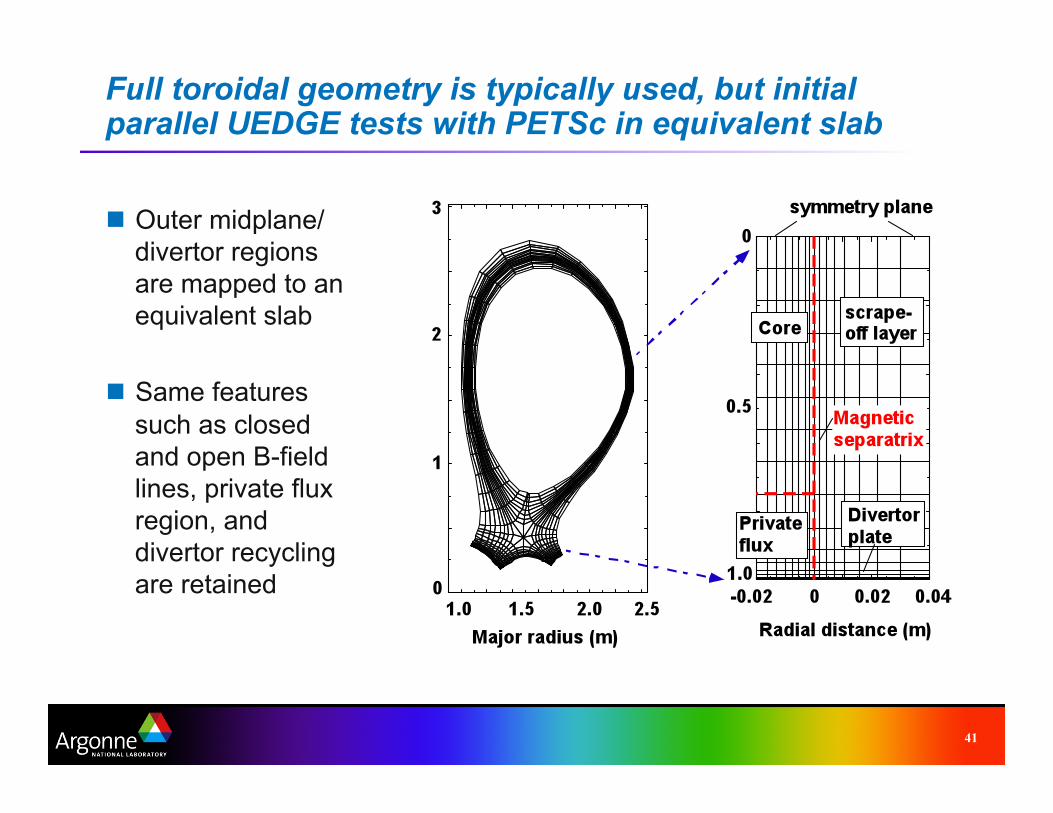
Full toroidal geometry is typically used, but initial parallel UEDGE tests with PETSc in equivalent slab

 Outer midplane/ divertor regions are mapped to an equivalent slab

  Same features such as closed and open B-field lines, private flux region, and divertor recycling are retained

41

Creating a DA

DACreate2d(comm, wrap, type, M, N, m, n, dof, s, lm[], ln[], *da)

wrap: Specifies periodicity DA_NONPERIODIC, DA_XPERIODIC, DA_YPERIODIC, …

type: Specifies stencil DA_STENCIL_BOX, DA_STENCIL_STAR

M/N: Number of grid points in x/y-direction m/n: Number of processes in x/y-direction s: The stencil width lm/ln: Alternative array of local sizes

42

Ghost Values

43

Local node

data layout

To evaluate a local function f(x) , each process requires •  its local portion of the vector x •  its ghost values – bordering portions of x owned by neighboring processes.

Communication and Physical Discretization

44 data layout

Communication Data Structure

Creation Ghost Point

Data Structures Ghost Point

Updates

Local Numerical

Computation Geometric

Data

DA AO

DACreate( ) DAGlobalToLocal( ) Loops over I,J,K indices

stencil [implicit]

VecScatter AO VecScatterCreate( ) VecScatter( ) Loops over

entities

elements edges

vertices unstructured meshes

structured meshes 1

2

A DA is more than a Mesh

A DA contains topology, geometry, and an implicit Q1 discretization

It is used as a template to create  Vectors (functions)  Matrices (linear operator)

45

Creating the Mesh

  Generic object –  MeshCreate() –  MeshSetMesh()

  File input –  MeshCreatePCICE() –  MeshCreatePyLith()

  Generation –  MeshGenerate() –  MeshRefine() –  ALE: :MeshBuilder::createSquareBoundary

  Representation –  ALE::SieveBuilder::buildTopology() –  ALE::SieveBuilder::buildCoordinates()

  Partitioning and distribution –  MeshDistribute() –  MeshDistributeByFace()

46

Parallel Sieves

 Sieves use names, not numberings –  Numberings can be constructed on demand

 Overlaps relate names on different processes –  An overlap can be encoded by a Sieve

 Distribution of a Section pushes forward along the Overlap –  Sieves are distributed as “cone” sections

47

Sections associate data to submeshes

 Name comes from section of a fiber bundle –  Generalizes linear algebra paradigm

 Define restrict(), update()  Define complete()  Assembly routines take a Sieve and several

Sections –  This is called a Bundle

48

Section Types Section can contain arbitrary values  C++ interface is templated over value type  C interface has two value types

–  SectionReal –  SectionInt

Section can have arbitrary layout  C++ interface can place unknowns on any Mesh entity (Sieve

point) –  Mesh::setupField() parametrized by Discretization and

BoundaryCondition

 C interface has default layouts –  MeshGetVertexSectionReal() –  MeshGetCellSectionReal()

49

Section Assembly

First we do local operations: –  Loop over cells –  Compute cell geometry –  Integrate each basis function to produce an element

vector –  Call SectionUpdateAdd()

Then we do global operations: –  SectionComplete() exchanges data across overlap

• C just adds nonlocal values (C++ is flexible)

–  C++ also allows completion over arbitrary overlap

50

Framework for Multi-model Algebraic System

~petsc/src/snes/examples/tutorials/ex31.c, ex32.c

http://www-unix.mcs.anl.gov/petsc/petsc-as/snapshots/petsc-dev/tutorials/multiphysics/tutorial.html

51

Framework for Multi-model Algebraic System ~petsc/src/snes/examples/tutorials/ex31.c

A model "multi-physics" solver based on the Vincent Mousseau's reactor core pilot code:

There are three grids

52

DA1

DA2

DA3

Fluid

Thermal conduction

(cladding and core)

Fission (core)

/* Create the DMComposite object to manage the three grids/physics. */ DMCompositeCreate(app.comm,&app.pack); DACreate1d(app.comm,DA_XPERIODIC,app.nxv,6,3,0,&da1); DMCompositeAddDA(app.pack,da1); DACreate2d(app.comm,DA_YPERIODIC,DA_STENCIL_STAR,…,&da2); DMCompositeAddDA(app.pack,da2); DACreate2d(app.comm,DA_XYPERIODIC,DA_STENCIL_STAR,…,&da3); DMCompositeAddDA(app.pack,da3);

/* Create the solver object and attach the grid/physics info */ DMMGCreate(app.comm,1,0,&dmmg); DMMGSetDM(dmmg,(DM)app.pack); DMMGSetSNES(dmmg,FormFunction,0);

/* Solve the nonlinear system */ DMMGSolve(dmmg);

/* Free work space */ DMCompositeDestroy(app.pack); DMMGDestroy(dmmg);

53

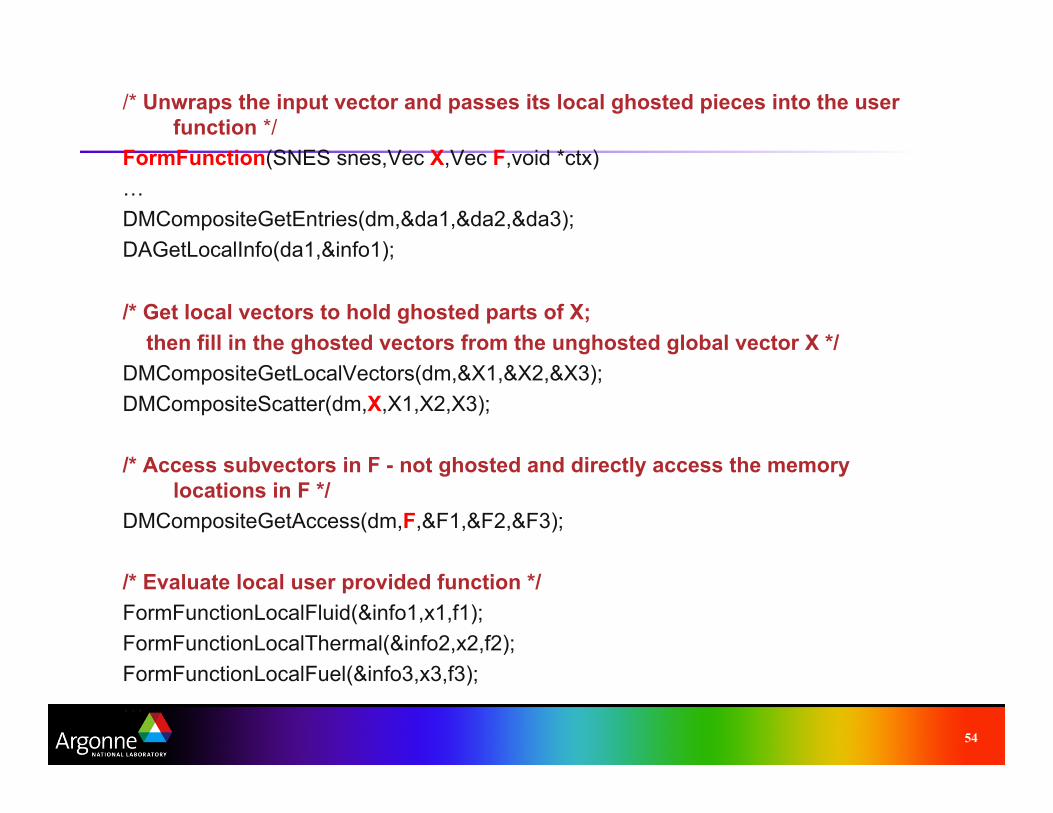
/* Unwraps the input vector and passes its local ghosted pieces into the user function */

FormFunction(SNES snes,Vec X,Vec F,void *ctx) … DMCompositeGetEntries(dm,&da1,&da2,&da3); DAGetLocalInfo(da1,&info1);

/* Get local vectors to hold ghosted parts of X; then fill in the ghosted vectors from the unghosted global vector X */ DMCompositeGetLocalVectors(dm,&X1,&X2,&X3); DMCompositeScatter(dm,X,X1,X2,X3);

/* Access subvectors in F - not ghosted and directly access the memory locations in F */

DMCompositeGetAccess(dm,F,&F1,&F2,&F3);

/* Evaluate local user provided function */ FormFunctionLocalFluid(&info1,x1,f1); FormFunctionLocalThermal(&info2,x2,f2); FormFunctionLocalFuel(&info3,x3,f3); …

54

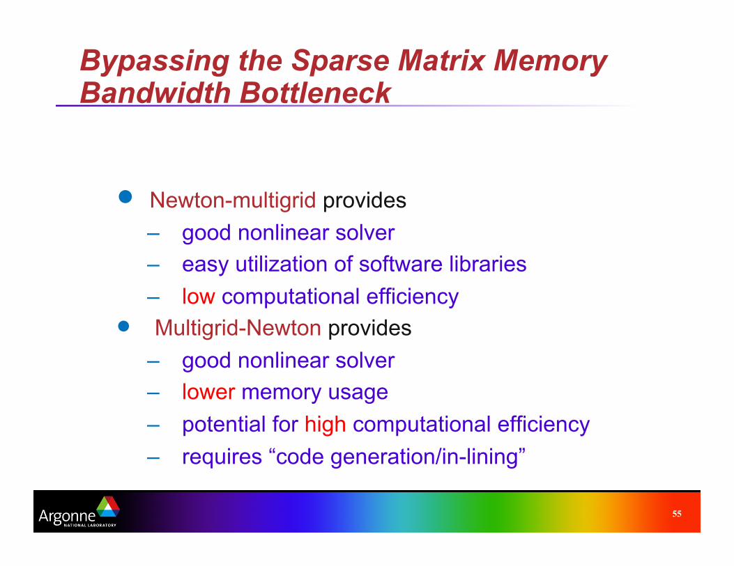
Bypassing the Sparse Matrix Memory Bandwidth Bottleneck

•  Newton-multigrid provides –  good nonlinear solver –  easy utilization of software libraries –  low computational efficiency

•  Multigrid-Newton provides –  good nonlinear solver –  lower memory usage –  potential for high computational efficiency –  requires “code generation/in-lining”

55

  Parallel Fast Poisson Solver

 More TS methods

 …

56

57

How will we solve numerical applications in 20 years?

•  Not with the algorithms we use today?

•  Not with the software (development) we use today?

How Can We Help?

 Provide documentation: –  http://www.mcs.anl.gov/petsc

 Quickly answer questions  Help install  Guide large scale flexible code development  Answer email at petsc-maint@mcs.anl.gov

58