i

P-RESONANT CONTROL FOR THE NEUTRAL POINT OF THREE PHASE

INVERTER

OMAR ALI OMAR AASHOUR

A thesis report submitted in partial

fulfillment of the requirement for the award of the

Degree of Master of Electrical and Electronic Engineering

Faculty of Electrical and Electronic Engineering

Universiti Tun Hussien Onn Malaysia

July, 2014

v

ABSTRACT

In this project, a Proportional resonant (PR) current controller is proposed to

maintain a balanced neutral point for a three-phase four wire inverter, which can be

used in microgrid applications. The neutral-point circuit consists of a conventional

neutral leg and a split DC link. The neutral point is balanced with respect to the two

DC source terminals (as required, in neutral-point clamped three-level converters)

even when the neutral current is large so that the inverter can be connected to an

unbalanced load. The controller, designed by using the Proportional resonant control

techniques, which attain eliminate for the current flowing through the split

capacitors. This leads to very small variation of the neutral point from the mid-point

of the DC source, in spite of the possibly large neutral current. The simulation of

inverter circuit, neutral-point and P-resonant has been performed using

MATLAB/SIMULINK software. The simulation results confirm the validity of the

proposed method, which can be seen as a promising that ensure P-resonant control

suitable for microgrid applications.

vi

ABSTRAK

Dalam projek ini, satu “Kadavan Hunan” pengawal arus bertujuan untuk

mengekalkan titik neutral seimbang untuk tiga fasa empat wayar penyongsang, yang

boleh digunakan dalam aplikasi microgrid. Litar pada titik neutral terdiri daripada

kaki neutral konvensional dan kepada sambungan perpecahan di DC. Titik neutral

adalah seimbang diantara dua terminal sumber pada DC (seperti yang dikehendaki,

dalam penukar tiga tahap titik cengkam neutral) walaupun semasa neutral adalah

besar supaya penyongsang boleh disambungkan kepada beban yang tidak seimbang.

Pengawal direka menggunakan teknik kawalan salunan berkadar, yang akan

menghapuskan arus yang melalui diantara celahan kapasitor. Keadaan ini akan

membawa kepada perubahan yang sangat kecil di titik neutral dari titik pertengahan

sumber DC, walaupun semasa neutral arusnya berkeadaan tinggi. Simulasi litar

penyongsang, titik neutral dan P-salunan telah dilakukan dengan menggunakan

perisian MATLAB / SIMULINK. Keputusan simulasi mengesahkan kesahihan

kaedah yang dicadangkan, yang boleh dilihat sebagai satu cara untuk memastikan

kawalan P-salunan sesuai untuk aplikasi microgrid.

ii

CONTENTS

ABSTRACT i

CONTENTS ii

LIST OF FIGURES iii

CHAPTER 1 INTRODUCTION

1.1 Project Background 1

1.2 Problem statement 3

1.3 project Objective 4

1.4 Scope of project 4

CHAPTER 2 LITERATURE REVIEW

2.1 Introduction 5

2.2 Inverters 5

2.2.1 Voltage Source Inverter 6

2.2.2 Current Source Inverter 7

2.3.1 Three-Phase Inverter 7

2.3.2 Sinusoidal PWM in Three-Phase Voltage Source

Inverters 9

2.3.3 Neutral point connection 11

2.3.3.1 The split DC link 12

2.3.3.2 Additional neutral leg 13

ii

2.3.3.3 The combination of first topology

and second topology 14

2.4 Controller 15

2.4.1 Open-loop control systems 15

2.4.2 Closed-loop control systems 15

2.5 Controllers for neutral point application 17

2.5.1 P Controller 18

2.5.2 PD Controller 18

2.5.3 Proportional integral controller 19

2.5.4 PID controller 20

2.5.5 Fuzzy logic controller 21

2.5.6 Control 23

2.6 P+Resonant controller 25

2.7 Three Phase Inverter in P+resonant 27

CHAPTER 3: METHODOLOGY

3.1 Introduction 28

3.2 Project block diagram 30

3.3 Generate SPWM switching using MATLAB Simulink 31

3.4 Inverter circuit design using MATLAB Simulink 32

3.5 Modeling of the neutral line circuit 33

CHAPTER 4: RESULT AND ANALYSIS

4.1 Introduction 37

4.2 System design and simulation 37

4.3.1 DC source model 38

4.3.2 The companion of neutral point leg and split of DC link

Model 39

ii

4.3.3 Three phase inverter controller model 40

4.3.4 P+ resonant current controller model 40

4.4 Software simulation results 41

4.4.1 Data simulation results 41

4.4.1.1 At reference current = 0 41

4.4.1.2 At reference current = 2 45

4.4.1.1 At reference current = 5 47

CHAPTER 5: CONCLUSION AND RECOMMENDATION

5.1 Project Conclusion 50

5.2 Recommendation 50

REFERENCES 52

x

LIST OF FIGURES

2.1 Voltage Source Inverter 6

2.2 Current Source Inverter (CSI) 7

2.3 Three-Phase Half Bridge Inverter 7

2.4 Three-phase Full –Bridge Inverter 8

2.5 Block diagram for generation of SPWM pulses 8

2.6 PWM illustration by the sine-triangle comparison method 9

2.7 Carrier & Reference Waveform along with the pulses of Sinusoidal

Pulse Width Modulation 10

2.8 Three-phase inverter network 11

2.9 The split DC link 12

2.10 Additional neutral leg 13

2.11 The combination 13

2.12 Open loop control system 14

2.13 Block diagram of a closed loop control system 15

2.14 Closed loop control system 16

2.15 Basic control systems 16

2.16 PI controller block diagram 18

2.17 A block diagram of a PID controller in a feedback loop 20

2.18 Fuzzy logic controller 21

xi

2.19 The standard optimal control problem 23

2.20 P-resonant controller 23

2.21 Inverter current mode controller block diagram 24

2.22 Frequency response characteristic of the open loop P-resonant

Controller 26

3.1 Project flow chart 28

3.2 Project block diagram 29

3.3 Flowchart of Generate SPWM switching using MATLAB Simulink 30

3.4 Flowchart of designing inverter circuit using MATLAB Simulink 32

3.5 Circuit topologies to generate a neutral 32

3.6 The firing pulse p and the inductor voltage 34

3.7 The block diagram of the neutral leg 35

4.1 System design and simulation 38

4.2 The DC source 38

4.3 The companion of neutral point leg and split of DC link model 39

4.4 Three phase inverter controller model 39

4.5 P-resonant current control and Pulse Withed Modulation (PWM) 40

4.6 P- resonant current control 40

4.7 Simulation open loop neutral point three phase inverter by using

MATLAB software 41

4.8 Output current for open loop circuit neutral point three phase inverter 42

4.9 Output voltage for open loop circuit neutral point three phase inverter 42

4.10 Capacitor current for open loop circuit neutral point three phase inverter 43

4.11 Inductor current for open loop circuit neutral point three phase inverter 43

4.12 Comparison of currents ( , and ) when: reference Current = 0A 45

4.13 Waveform of control signal of p-resonant controller when

reverence value =0 46

xii

4.14 Waveform of generate two pulses PWM when reverence value =0 46

4.15 Three phase current load Iabc 47

4.16 Three phase voltage load Vabc 47

4.17 Comparison of currents ( , and ) when: reference Current = 2 49

4.18 Three phase current load Iabc 49

4.19 Three phase voltage load Vabc 50

4.20 Comparison of currents ( , and ) when: reference Current = 5 51

4.21 Three phase current load Iabc 52

4.22 Three phase voltage load Vabc 52

xiii

LIST OF SYMBOLS AND ABBREVIATIONS

DC direct current

AC alternating current

VFI voltage fed inverter

VSI voltage source inverter

CSI Current source inverter

PR Proportional Resonant

PWM Pulse Width Modulation

ASDs adjustable speed drives

SPWM sinusoidal pulse-width modulation

VSCs voltage-source converters

PI Proportional integral

PID Proportional Integral Derivative

PD Proportional Derivative

FLC Fuzzy logic controller

SVM Space Vector Modulation

CHAPTER 1

INTRODUCTION

1.1 Project Background

A power inverter is an electrical power converter that changes direct current (DC) to

alternating current

(AC); the converted AC can be at any required voltage and frequency with the use

of appropriate transformers, switching, and control circuits [1]. A typical power

inverter device or circuit will require a relatively stable DC power source capable of

supplying enough current for the intended overall power handling of the inverter.

Possible DC power sources include: rechargeable batteries, DC power supplies

operating off of the power company line, and solar cells. The inverter does not

produce any power, the power is provided by the DC source. The inverter translates

the form of the power from direct current to an alternating current waveform. The

level of the needed input voltage depends entirely on the design and purpose of the

inverter. In many smaller consumer and commercial inverters a 12V DC input is

popular because of the wide availability of powerful rechargeable 12V lead acid

batteries which can be used as the DC power source. A power inverter device which

produces a smooth sinusoidal AC waveform is referred to as a sine wave inverter. To

more clearly distinguish from "modified sine wave" or other creative terminology,

the phrase pure sine wave inverter is sometimes used. In situations involving power

inverter devices which substitute for standard line power, a sine wave output is

extremely desirable because the vast majority of electric plug in products and

appliances are engineered to work well with the standard electric utility power which

is a true sine wave. At present, sine wave inverters tend to be more complex and

2

have significantly higher cost than a modified sine wave type of the same power

handling.

Three-phase inverters are used for variable-frequency drive applications and

for high power applications such as HVDC power transmission. A basic three-phase

inverter consists of three single-phase inverter switches each connected to one of the

three load terminals. For the most basic control scheme, the operation of the three

switches is coordinated so that one switch operates at each 60 degree point of the

fundamental output waveform. This creates a line-to-line output waveform that has

six steps. The six-step waveform has a zero-voltage step between the positive and

negative sections of the square-wave such that the harmonics that are multiples of

three are eliminated as described above. When carrier-based PWM techniques are

applied to six-step waveforms, the basic overall shape, or envelope, of the waveform

is retained so that the harmonic and its multiples are cancelled[2].

Inverters can be broadly classified into two types, voltage source and

current source inverters. A voltage fed inverter (VFI) or more generally a voltage–

source inverter (VSI) is one in which the DC source has small or negligible

impedance. The voltage at the input terminals is constant. A current–source

inverter (CSI) is fed with adjustable current from the DC source of high

impedance that is from a constant DC source. A voltage source inverter

employing thyristors as switches, some type of forced commutation is required,

while the (VSI) made up of using GTOs, power transistors, power MOSFETs or

IGBTs, self-commutation with base or gate drive signals for their controlled turn-

on and turn-off.

Since the neutral point of an electrical supply system is often connected to

neutral, under certain conditions, a conductor used to connect to a system neutral is

also used for grounding of equipment and structures. Current carried on a grounding

conductor can result in objectionable or dangerous voltages appearing on equipment

enclosures, so the installation of grounding conductors and neutral conductors is

carefully defined in electrical regulations. Where a neutral conductor is used also to

connect equipment enclosures to earth, care must be taken that the neutral conductor

never rises to a high voltage with respect to local ground.

Proportional Resonant (PR) controller gained a large popularity in recent

years in current regulation of grid-tied systems. It introduces an infinite gain at a

selected resonant frequency for eliminating steady-state error or current harmonics at

3

that frequency. However the harmonic compensators of the proportional resonant

controllers are limited to several low-order current harmonics, due to the system

instability when the compensated frequency is out of the bandwidth of the

systems[3].

1.2 Problem Statements

Many power electronics applications, such as Distributed Generation systems,

Uninterruptible Power Supplies or active filtering, employ an inverter feeding a star

connected three-phase load with accessible neutral terminal. The currents flowing on

each phase are generally not balanced so, if a transformer is not required, a

connection to the neutral terminal should be provided by adding an extra wire to the

inverter.

The neutral line is usually needed to provide a current path for possible

unbalanced loads and the traditional six-switch inverter must be supplemented with a

neutral connection. If the neutral point of a four-wire system is not well balanced,

then the neutral-point voltage may deviate severely from the real midpoint of the DC

source. This deviation of the neutral point may result in an unbalanced or variable

output voltage, the presence of the DC component, larger neutral current or even

more serious problems. Thus, the generation of a balanced neutral point in a simple

and effective manner has become an important issue.

1.3 Project Objectives

i. To develop and simulate the neutral point connection for DC-AC inverter.

ii. To develop proportional resonant controller that suitable for neutral point

for three phase inverter.

iii. To have zero current flows for the capacitor link at neutral point.

1.4 Project Scopes

i. Modelling of three phase DC-AC inverter with neutral point connection that

will be modelled using MATLAB Simulink software.

4

ii. P-resonant control with Sinusoidal Pulse Width Modulation (SPWM)

technique will be used to control the switching signals for the switches at

neutral point connection

iii. Using the P-resonant control technique as controller to reduce the current

flow at capacitor link in neutral point using MATLAB.

CHAPTER 2

LITERATURE REVIEW

2.1 Introduction

This chapter is a general introduction to the neutral point of three phase inverter and

it also focus on proportional resonant controller. The basic components and their

detailed functions will be introduced and discussed.

2.2 Inverters

Inverters can be found in a variety of forms, including half bridge or full bridge,

single phase or three phases. In pulse width modulated (PWM) inverters the input

DC voltage is essentially constant in magnitude and the AC output voltage has

controlled magnitude and frequency. Therefore the inverter must control the

magnitude and the frequency of the output voltage. This is achieved by PWM of the

converter switches and hence such converters are called PWM converters.

The DC-AC inverters usually operate on Pulse Width Modulation (PWM)

technique. The PWM is a very advance and useful technique in which width of the

gate pulses are controlled by various mechanisms. PWM inverter is used to keep the

output voltage of the inverter at the rated voltage (depending on the user’s choice)

irrespective of the output load. In a conventional inverter the output voltage changes

according to the changes in the load. To nullify this effect of the changing loads, the

PWM inverter correct the output voltage by changing the width of the pulses and the

output AC depends on the switching frequency and pulse width which is adjusted

6

according to the value of the load connected at the output so as to provide constant

rated output.

2.2.1 Voltage Source Inverter

The type of inverter that most commonly used is voltage source inverter (VSI) where

AC power provides on the output side function as a voltage source. The input DC

voltage may be an independent source such as battery, which is called a ’DC link’

inverter. These structure are the most widely used because they naturally behave as

voltage source as required by many industrial application, such as adjustable speed

drives (ASDs), which are the most popular application of inverters Figure2.1 shows

the voltage source inverter. Single phase VSIs are used in low range power

application where the three phase VSIs is used in medium to high-power application.

The main purposes of three-phase VSIs are to provide a three-phase voltage source,

where the amplitude, phase and frequency of the voltage should be controllable [4].

Figure2.1: Voltage Source Inverter (VSI)

2.2.2 Current Source Inverter

Respectively, CSI the DC source appears as a constant current and the voltage is

changing with the load. The protection filter is normally a capacitance in parallel

with the DC source The main advantage of the current source inverter is that it

increases the voltage towards the mains itself. Figure 2.2 shows the current source

inverter [5].

7

Figure2.2: Current Source Inverter (CSI)

2.3.1 Three-Phase Inverter

The dc to ac converters more commonly known as inverters, depending on the type

of the supply source and the related topology of the power circuit, are classified as

voltage source inverters (VSIs) and current source inverters (CSIs). Three-phase

counterparts of the single-phase half and full bridge voltage source inverters are

shown in Figures 2.3 and 2.4. Single-phase VSIs cover low-range power applications

and three-phase VSIs cover medium to high power applications. The main purpose of

these topologies is to provide a three-phase voltage source, where the amplitude,

phase and frequency of the voltages can be controlled. The three-phase dc/ac voltage

source inverters are extensively being used in motor drives, active filters and unified

power flow controllers in power systems and uninterrupted power supplies to

generate controllable frequency and ac voltage magnitudes using various pulse width

modulation (PWM) strategies. The standard three-phase inverter shown in Figure 2.4

has six switches the switching of which depends on the modulation scheme. The

input dc is usually obtained from a single-phase or three phase utility power supply

through a diode-bridge rectifier and LC or C filter.

a

b

c

+ Van -

+ Vbn -

+ Vcn -

n+

O

C

C

S11

S12

S21

S22

VDC

Figure 2.3: Three-Phase Half Bridge Inverter

8

a

b

c

+ Van -

+ Vbn -

+ Vcn -

n+

O

S11

S12

S21

S22

S31

S32

VDC

Figure 2.4: Three-phase Full –Bridge Inverter

2.3.2 Sinusoidal PWM in Three-Phase Voltage Source Inverters

The voltage source inverter that use PWM switching techniques have a DC input

voltage ( = ) that is usually constant in magnitude. The inverter job is to take

this DC input and to give AC output, where the magnitude and frequency can be

controlled. There are several techniques of Pulse Width Modulation (PWM). The

efficiency parameters of an inverter such as switching losses and harmonic reduction

are principally depended on the modulation strategies used to control the inverter[6].

The sinusoidal pulse-width modulation (SPWM) technique produces a sinusoidal

waveform by filtering an output pulse waveform with varying width. A high

switching frequency leads to a better filtered sinusoidal output waveform. The

variations in the amplitude and frequency of the reference voltage change the pulse-

width patterns of the output voltage but keep the sinusoidal modulation. As shown in

Figure 2.5.

Figure 2.5: Block diagram for generation of SPWM pulses

9

As in the single phase voltage source inverters PWM technique can be used

in three-phase inverters, in which three sine waves phase shifted by 120° with the

frequency of the desired output voltage is compared with a very high frequency

carrier triangle, the two signals are mixed in a comparator whose output is high when

the sine wave is greater than the triangle and the comparator output is low when the

sine wave or typically called the modulation signal is smaller than the triangle. This

phenomenon is shown in Figure 2.6. As is explained the output voltage from the

inverter is not smooth but is a discrete waveform and so it is more likely than the

output wave consists of harmonics, which are not usually desirable since they

deteriorate the performance of the load, to which these voltages are applied [7].

Figure 2.6: PWM illustration by the sine-triangle comparison method (a) sine-

triangle comparison (b) switching pulses.

The gating signals can be generated using unidirectional triangular carrier

wave as shown in the Figure2.7 But a pulse width modulated inverter employing

pure sinusoidal modulation cannot supply sufficient voltage to enable a standard

motor to operate at rated power and rated speed. Sufficient voltage can be obtained

from the inverter by over modulating, but this produces distortion of the output

10

waveform. The linear output range of SPWM is restricted to 0.785 compared with six

step inverter. The non-linear region operation (over-modulation) is leading to large

amounts of sub carrier frequency harmonic currents, reduction in fundamental

voltage gain and switching device gate pulse dropping [8].

Figure 2.7: Carrier & Reference Waveform along with the pulses of Sinusoidal

Pulse Width Modulation

2.3.3 Neutral point connection

The principles for the physical layout of three phase inverters, also known as

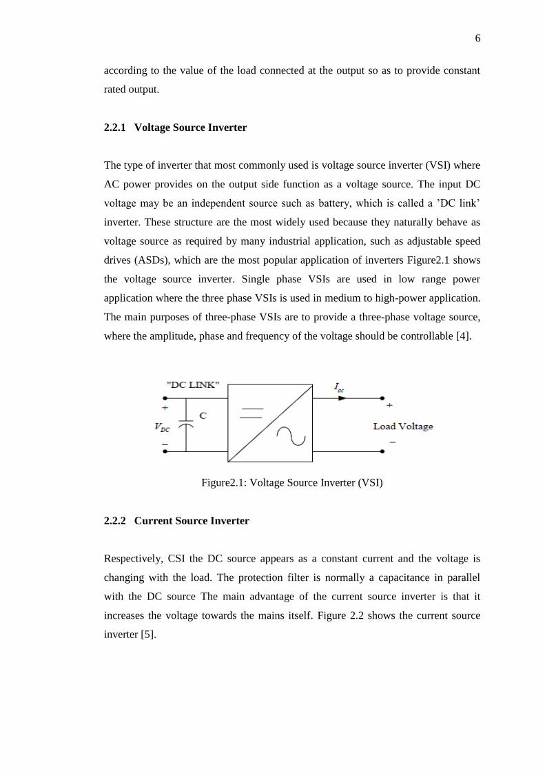
voltage-source converters (VSC:s) are shown in Figure 2.8 The bridge is connected

to the DC-link, whose voltage is raw material in the creation of the three-phase

output voltage. The link voltage is from now on called dc-link. The mid potential of

the dc-link is defined as neutral

11

LOAD

Va

Vb

Vc

2

DCV

2

DCV

Figure 2.8: Three-phase inverter network.

Between the two poles of the dc link, the three half-bridges are connected. Each half

bridge has two power electronic switches. By switching them, between fully

conducting and fully blocking, the potentials of each half-bridge ( , , , with

respect to the mid potential of the dc link, can attain /2 ± .

This deviation of the neutral point may result in an unbalanced or variable

output voltage, the presence of the DC component, larger neutral current or even

more serious problems. Thus, the generation of balanced neutral point in a simple

and effective manner has become an important issue. The neutral-point circuit

consists of a conventional neutral leg and a split DC link. The neutral point is

balanced with respect to the two DC source terminals (as required, e.g., in neutral

point clamped three-level converters) even when the neutral current is large so that

the inverter can be connected to an unbalanced load and/or utility grid. Three

different circuit topologies have been widely used to generate a neutral point [9].

2.3.3.1 The split DC link

The first topology is a split DC link as shown in Figure 2.9, with the neutral point

clamped at half of the DC link voltage. Since the neutral current flows through

capacitors, high capacitance is necessary. Moreover, the neutral point usually shifts

following capacitors and/or switches differences. To improve performance of the

split DC link topology, different neutral point balancing strategies are reported,

usually using redundant states of the Space Vector Pulse Width Modulation

(SVPWM). In this solution, in is certainly the simplest one, but the three-phase

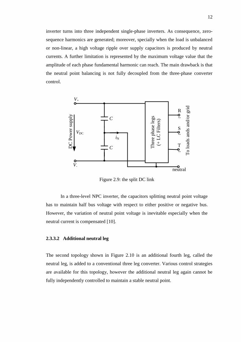
12

inverter turns into three independent single-phase inverters. As consequence, zero-

sequence harmonics are generated; moreover, specially when the load is unbalanced

or non-linear, a high voltage ripple over supply capacitors is produced by neutral

currents. A further limitation is represented by the maximum voltage value that the

amplitude of each phase fundamental harmonic can reach. The main drawback is that

the neutral point balancing is not fully decoupled from the three-phase converter

control.

R

S

T

~

~

~

neutral

iN

Th

ree

ph

ase

leg

s

(+ L

C F

ilte

rs) C

DC

Po

wer

su

pp

ly

VDC

V+

V-

To

lo

ads

and

s an

d/o

r g

rid

C

Figure 2.9: the split DC link

In a three-level NPC inverter, the capacitors splitting neutral point voltage

has to maintain half bus voltage with respect to either positive or negative bus.

However, the variation of neutral point voltage is inevitable especially when the

neutral current is compensated [10].

2.3.3.2 Additional neutral leg

The second topology shown in Figure 2.10 is an additional fourth leg, called the

neutral leg, is added to a conventional three leg converter. Various control strategies

are available for this topology, however the additional neutral leg again cannot be

fully independently controlled to maintain a stable neutral point.

13

R

S

T

~

~

~

neutral

LN

C

S7

S8

DC

Pow

er s

upply

VDC

V+

V-

To l

oad

s an

ds

and

/or

gri

d

Thre

e phas

e le

gs

(+ L

C F

ilte

rs)

Figure 2.10: additional neutral leg

2.3.3.3 The combination of first topology and second topology.

The third topology, an actively balanced split DC link topology shown in Figure

2.11, is the combination of the first two (split DC link and the additional neutral

leg).The control of the neutral point in this case can be decoupled from the control of

the three phase converter [11].

R

S

T

~

~

~

neutral

iL LNiN

N

ic

Thre

e phas

e le

gs

(+ L

C F

ilte

rs) CN

CN

uN

S7

P

P

S8

DC

Pow

er s

upply

VDC

V+

V-

To l

oad

s an

ds

and

/or

gri

d

Figure 2.11: The combination of .2.9: and 2.10: the actively balanced split DC link

14

2.4 Controller

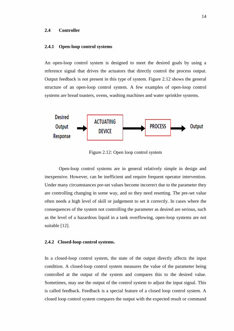
2.4.1 Open-loop control systems

An open-loop control system is designed to meet the desired goals by using a

reference signal that drives the actuators that directly control the process output.

Output feedback is not present in this type of system. Figure 2.12 shows the general

structure of an open-loop control system. A few examples of open-loop control

systems are bread toasters, ovens, washing machines and water sprinkler systems.

Figure 2.12: Open loop control system

Open-loop control systems are in general relatively simple in design and

inexpensive. However, can be inefficient and require frequent operator intervention.

Under many circumstances pre-set values become incorrect due to the parameter they

are controlling changing in some way, and so they need resetting. The pre-set value

often needs a high level of skill or judgement to set it correctly. In cases where the

consequences of the system not controlling the parameter as desired are serious, such

as the level of a hazardous liquid in a tank overflowing, open-loop systems are not

suitable [12].

2.4.2 Closed-loop control systems.

In a closed-loop control system, the state of the output directly affects the input

condition. A closed-loop control system measures the value of the parameter being

controlled at the output of the system and compares this to the desired value.

Sometimes, may use the output of the control system to adjust the input signal. This

is called feedback. Feedback is a special feature of a closed loop control system. A

closed loop control system compares the output with the expected result or command

15

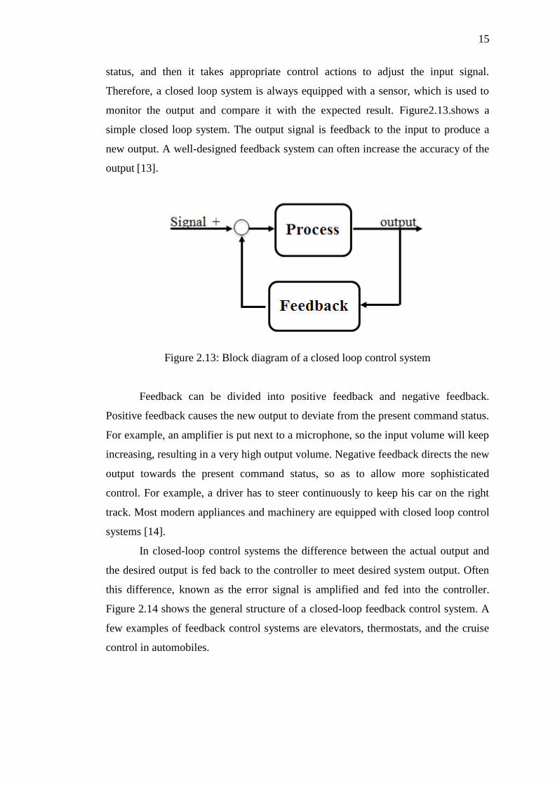
status, and then it takes appropriate control actions to adjust the input signal.

Therefore, a closed loop system is always equipped with a sensor, which is used to

monitor the output and compare it with the expected result. Figure2.13.shows a

simple closed loop system. The output signal is feedback to the input to produce a

new output. A well-designed feedback system can often increase the accuracy of the

output [13].

Figure 2.13: Block diagram of a closed loop control system

Feedback can be divided into positive feedback and negative feedback.

Positive feedback causes the new output to deviate from the present command status.

For example, an amplifier is put next to a microphone, so the input volume will keep

increasing, resulting in a very high output volume. Negative feedback directs the new

output towards the present command status, so as to allow more sophisticated

control. For example, a driver has to steer continuously to keep his car on the right

track. Most modern appliances and machinery are equipped with closed loop control

systems [14].

In closed-loop control systems the difference between the actual output and

the desired output is fed back to the controller to meet desired system output. Often

this difference, known as the error signal is amplified and fed into the controller.

Figure 2.14 shows the general structure of a closed-loop feedback control system. A

few examples of feedback control systems are elevators, thermostats, and the cruise

control in automobiles.

16

Figure 2.14: Closed loop control system.

2.5 Controllers for neutral point application

PID controllers use a three basic behaviour types or modes: P - proportional, I -

integrative and D - derivative. While proportional and integrative modes are also

used as single control modes, a derivative mode is rarely used on its own in control

systems. Combinations such as PI and PD control are very often in practical systems

Figure 2.15: basic control systems

2.5.1 P Controller

In general can say P controller cannot stabilize higher order processes. For order

processes, the meaning of processes with one energy storage, a large increasing the

gain can be tolerated. Proportional controller can stabilize only 1st order unstable

process. Therefore, can change the gain of controlled can change closed loop system.

17

And large gain of controlled will result in control system with steady state error is

small, better reference following, Faster dynamics, broader signal frequency band of

the closed loop system and larger sensitivity with respect to measuring noise, and

Phase margin and smaller amplitude.

When P controller is used, there will be a dire need to have a large gain to

large gain to improve steady state error. Stable systems do not have problems when

large gain is used. Such systems are systems energy storage ( order capacitive

systems).If steady state error is constant can be accepted with such processes, than P

controller can be used. Small steady state errors can be accepted if sensor will give

measured value with error or if importance of measured value is not too great

anyway [15].

2.5.2 PD Controller

D is used when prediction of the error can improve control or when it necessary to

stabilize the system. From the frequency characteristic of D element it can be seen

that it has phase lead of 90°

To avoid effects of the sudden change of the reference input that will cause

sudden change in the value of error signal. That is why is not taken from the error

signal but from the system output variable. Sudden change in error signal will cause

sudden change in control output. To avoid that it is suitable to design D mode to be

proportional to the change of the output variable.

Always PD control used for moving objects such are flying and underwater

vehicles, ships, rockets etc.

2.1

2.5.3 Proportional integral controller

A Proportional Integral (PI) control is a special case of the classic controller family

known as Proportional Integral Derivative (PID). These types of controllers are up to

date the most common way of controlling industry processes in a feedback

configuration. More than 95% of all installed controllers are PID [16]. PI controller

has some disadvantages such as: high starting overshoot, sensitivity to controller

18

gains and sluggish response due to sudden load disturbance. A PI controller is a

controller that produces proportional plus integral control action. The PI controller

has only one input and one output. The output value increases when the input value

increases. Figure 2.16 shows the Proportional-Integral (PI) controller block diagram.

Figure 2.16: PI controller block diagram

PI control is a traditional linear control method used in industrial

applications. The linear PI controller controllers are usually designed for dc-ac

inverter and dc-dc converters using standard frequency response techniques and

based on the small signal model of the converter. A Bode plot is used in the design to

obtain the desired loop gain, crossover frequency and phase margin. The stability of

the system is guaranteed by an adequate phase margin. However, linear PID and PI

controllers can only be designed for one nominal operating point. A boost

converter’s small signal Model changes when the operating point varies. The poles

and a right-half plane zero, as well as the magnitude of the frequency response, are

all dependent on the duty cycle. Therefore, it is difficult for the PID controller to

respond well to changes in operating point. The PI controller is designed for the

boost converter for operation during a start-up transient and steady state respectively

[17].

2.2

19

2.5.4 PID controller

Proportional-integral-derivative controller (PID controller) is a generic control loop

feedback mechanism (controller) widely used in industrial control systems. A PID

controller calculates an "error" value as the difference between a measured process

variable and a desired set point. The controller attempts to minimize the error by

adjusting the process control inputs. Calculation (algorithm) involves three separate

constant parameters, and is accordingly sometimes called three-term control: the

proportional, the integral and derivative values, denoted P, I, and D. Heuristically,

these values can be interpreted in terms of time: P depends on the present error, I on

the accumulation of past errors, and D is a prediction of future errors, based on

current rate of change. The weighted sum of these three actions is used to adjust the

process via a control element such as the position of a control valve, a damper, or the

power supplied to a heating element.

In the absence of knowledge of the underlying process, a PID controller

has historically been considered to be the best controller. By tuning the three

parameters in the PID controller algorithm, the controller can provide control

action designed for specific process requirements. The response of the controller

can be described in terms of the responsiveness of the controller to an error, the

degree to which the controller overshoots the set point and the degree of system

oscillation. Note that the use of the PID algorithm for control does not guarantee

optimal control of the system or system stability.

2.3

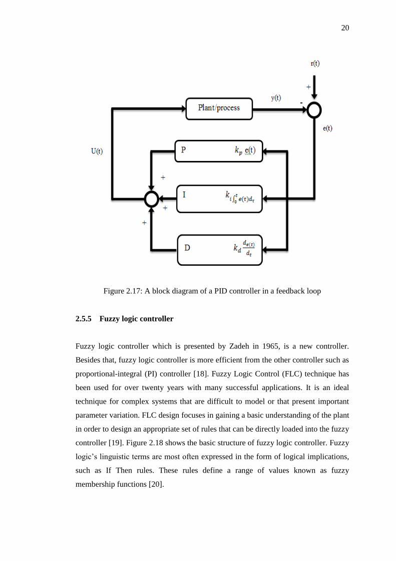
20

Figure 2.17: A block diagram of a PID controller in a feedback loop

2.5.5 Fuzzy logic controller

Fuzzy logic controller which is presented by Zadeh in 1965, is a new controller.

Besides that, fuzzy logic controller is more efficient from the other controller such as

proportional-integral (PI) controller [18]. Fuzzy Logic Control (FLC) technique has

been used for over twenty years with many successful applications. It is an ideal

technique for complex systems that are difficult to model or that present important

parameter variation. FLC design focuses in gaining a basic understanding of the plant

in order to design an appropriate set of rules that can be directly loaded into the fuzzy

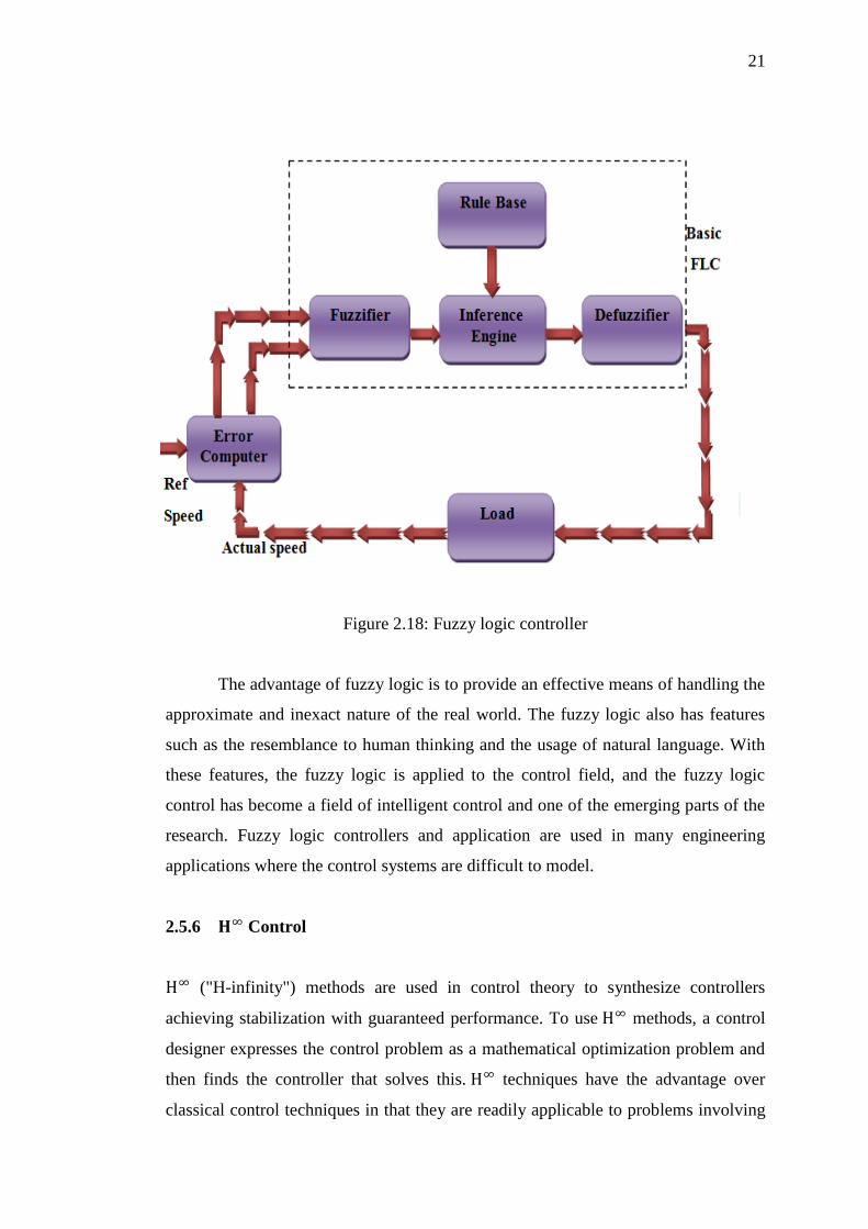
controller [19]. Figure 2.18 shows the basic structure of fuzzy logic controller. Fuzzy

logic’s linguistic terms are most often expressed in the form of logical implications,

such as If Then rules. These rules define a range of values known as fuzzy

membership functions [20].

21

Figure 2.18: Fuzzy logic controller

The advantage of fuzzy logic is to provide an effective means of handling the

approximate and inexact nature of the real world. The fuzzy logic also has features

such as the resemblance to human thinking and the usage of natural language. With

these features, the fuzzy logic is applied to the control field, and the fuzzy logic

control has become a field of intelligent control and one of the emerging parts of the

research. Fuzzy logic controllers and application are used in many engineering

applications where the control systems are difficult to model.

2.5.6 Control

("H-infinity") methods are used in control theory to synthesize controllers

achieving stabilization with guaranteed performance. To use methods, a control

designer expresses the control problem as a mathematical optimization problem and

then finds the controller that solves this. techniques have the advantage over

classical control techniques in that they are readily applicable to problems involving

22

multivariable systems with cross-coupling between channels; disadvantages of

techniques include the level of mathematical understanding needed to apply them

successfully and the need for a reasonably good model of the system to be controlled.

It is important to keep in mind that the resulting controller is only optimal with

respect to the prescribed cost function and does not necessarily represent the best

controller in terms of the usual performance measures used to evaluate controllers

such as settling time, energy expended, etc. Also, non-linear constraints such as

saturation are generally not well-handled.

The phrase control comes from the name of the mathematical space over

which the optimization takes place: is the space of matrix-valued functions that

are analytic and bounded in the open right-half of the complex plane defined by

Re(s) > 0; the norm is the maximum singular value of the function over that

space. (This can be interpreted as a maximum gain in any direction and at any

frequency; for SISO systems, this is effectively the maximum magnitude of the

frequency response). Techniques can be used to minimize the closed loop impact

of a perturbation: depending on the problem formulation, the impact will either be

measured in terms of stabilization or performance. Simultaneously optimizing robust

performance and robust stabilization is difficult. One method that comes close to

achieving this is loop-shaping, which allows the control designer to apply

classical loop-shaping concepts to the multivariable frequency response to get good

robust performance, and then optimizes the response near the system bandwidth to

achieve good robust stabilization. First, the process has to be represented according

to the following standard configuration. In this section the and repetitive control

techniques are brie y introduced and the former work of the voltage controller design

is presented. The methods are used in control theory to synthesise controllers

achieving robust performance or stabilisation. The optimal control theory is an

effective method to design a controller to guarantee the performance with the worst-

case disturbance. Its basic principle is to minimise the influence of the disturbances

to outputs.

The standard optimal control problem is shown in Figure 2.19 where

represents an external disturbance, is the measurement available to the controller,

is the output from the controller, and is an error signal that it is desired to keep

small.

23

Figure 2.19: the standard optimal control problem

The plant P has two inputs, the exogenous input w, that includes reference

signal and disturbances, and the manipulated variables u. There are two outputs; the

error signals z that we want to minimize, and the measured variables v, that we use to

control the system. v is used in c to calculate the manipulated variable u.

2.6 P-Resonant controller

This controller aims to get a good reference tracking and to reduce the output voltage

harmonic distortion when the inverter feeds linear and nonlinear loads. The resonant

controller is a generalized PI controller that is able to control not only DC but also

AC variables. Figure 2.20 shows the structure of the resonant controller [21].

Figure 2.20: P-resonant controller

24

In addition to a forward integrator there is another integrator in the feedback loop.

The transfer function is given by

2.4

Where represents the resonance frequency of the integrator corresponding

to the signal’s fundamental frequency, is the Proportional gain, is the integral

gain of the controller. Proportional resonant controllers have infinite gain on the

resonant frequency and so they can get zero steady state error on the stationary

frame. The general concepts of Proportional resonant controller for single phase and

three phase inverters are the same and the difference is how to perform the variable

transformation to the alpha-beta frame and then back to the main domain, if required.

Here after explaining the general proportional resonant controller strategy, it will be

shown how to calculate the current reference and do the required transformations for

three phase and single phase inverter.

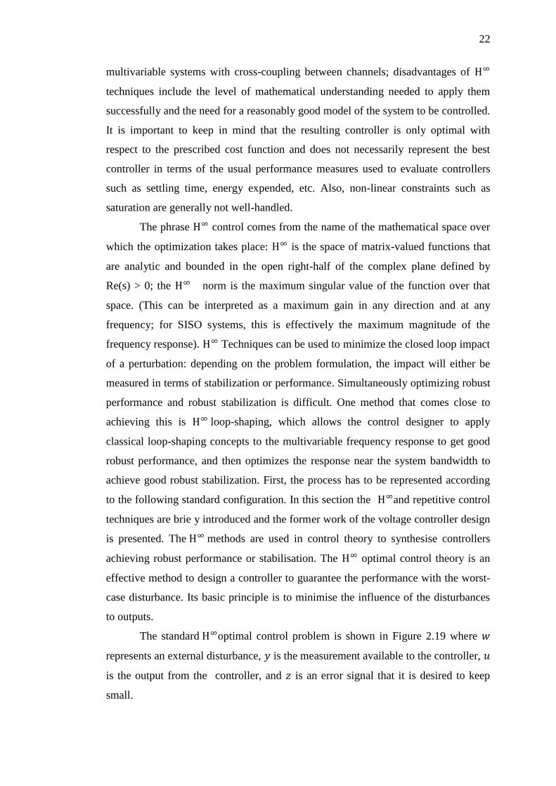
Here

is the resonant part whose resonant frequency is at and is

the proportional part. The resonant part is able to provide a very high gain at and

around the resonant frequency which forces the error to become zero at steady state

[22].

Assuming that

in dq frame, its equivalent in stationary frame will be

[22]:

2.5

The current controller block is shown in figure. 2.21

Figure 2.21: Inverter current mode controller block diagram

55

REFERENCES

1. Holmes, D. Grahame, and Thomas A. Lipo. Pulse width modulation for power

converters: principles and practice. Vol. 18. Wiley-IEEE Press, 2003.

2. Zhang, Yu, Yong Kang, and Jian Chen. "The zero-sequence circulating currents

between parallel three-phase inverters with three-pole transformers and

reactors." Applied Power Electronics Conference and Exposition, 2006. APEC'06.

Twenty-First Annual IEEE. IEEE, 2006.

3. M. Aredes, J. H¨afner and K. Heumann. “Three-Phase Four-Wire ShuntActive Filter

Control Strategies,” IEEE Transactions on Power Electronics,Vol.12(2), March

1997, pp. 311-318

4. Rahman, Abdullah Al Mahfazur, and Muhammad Usman Sabbir. "Grid Code

Testing by Voltage Source Converter." (2012).

5. Xiaorong, Xie, Yan Gangui, and Chen Yuanhua. "Matlab simulation platform for

three-level PWM variable-frequency speed-governing control system." POWER

SYSTEM TECHNOLOGY-BEIJING- 27.9 (2003): 18-22.

6. Salam, Zainal, Abdul Aziz, and Mohd Junaidi. "The Design and Development of a

High Perfomance Bi-directional Inverter For Photovoltaic Application." (2003).

7. Babaei E, Hosseini SH, Gharehpetian G., “Reduction of THD and low order

harmonics with symmetrical output current for single-phase ac/ac matrix converters.”

International Journal of Electrical Power& Energy System2010 – Elsevier; Volume

32, Issue 3, March 2010, Pages 225–235. (Article)

56

8. J. Holtz, “Pulse width modulation for electronic power conversion,” Proc. IEEE, vol.

82, pp. 1194–1214, Aug. 1994

9. P. Dharmadhikari, G. Goyal. “ Analysis & Hardware Implementation Of Three-

Phase Voltage Source Inverter”, International Journal of Engineering Research &

Technology (IJERT) ISSN: 2278-0181, Vol. 2 Issue 5, May - 2013

10. Q.C. Zhong, J. Liang, G. Weiss, C. Feng, and T. Green, “H1 control of the neutral

point in four-wire three-phase DC-AC converters,” IEEE Transactions on Industrial

Electronics, vol. 53, no. 5, pp. 1594–1602,2006

11. . X. Yuan, G. Orglmeister, andW. Merk, “Managing the DC link Neutral Potential of

the three-phase-four-wire neutral-point-clamped (NPC) inverter in FACTS

Application,” in Proc. IEEE Ind. Electron. Soc. Conf., 1999, pp. 571–576.

12. R. Zhang, D. Boroyevich, V. H. Prasad, H. Mao, F. C. Lee, and S. Dubovsky,“Three-

phase inverter with a neutral leg with space vectormodulation,” in IEEE 12th

Applied Power Electronics Conference,vol. 2, Atlanta, GA, USA, Feb. 1997, pp.

857–863.

13. Hart, John K. Automatic control program creation using concurrent Evolutionary

Computing. Diss. Bournemouth University, 2004.

14. Aström, Karl Johan, and Richard M. Murray. Feedback systems: an introduction for

scientists and engineers. Princeton university press, 2010.

15. M.Ali Akcayol, Aydin Cetin, and Cetin Elmas, (November 2002), An Educational

Tool for Fuzzy Logic-Controlled BDCM, IEEE Transaction on Education, vol. 45,

no. 1.

16. Luis Alberto Torres Salomao, Hugo Gámez Cuatzin, Juan Anzurez Marín and Isidro

I.Lázaro Castillo, ”Fuzzy-PI Control, PI Control and Fuzzy Logic Control

Comparison Applied to a Fixed Speed Horizontal Axis 1.5 MW Wind Turbine”,

57

Proceedings of the World Congress on Engineering and Computer Science 2012 Vol

II WCECS 2012, pp. 978-988-19252-4-4.

17. Hanns, Michael. “A Nearly Strict Fuzzy Arithmetic for Solving Problems

withUncertainties.” Online posting. 14 Dec. 2002

18. K.J. Åström and T.H. Hägglund, “New tuning methods for PID

controllers”,Proceedings of the 3rd European Control Conference, 1995, p.2456–62.

19. Ortega, R., et al. "A PI-P+ Resonant controller design for single phase inverter

operating in isolated microgrids." Industrial Electronics (ISIE), 2012 IEEE

International Symposium on. IEEE, 2012.

20. R. Teodorescu, F. Blaabjerg, U. Borup, and M. Liserre. A new control structure for

grid-connected lcl pv inverters with zero steady-state error and selective harmonic

compensation. In Applied Power Electronics Conference and Exposition, 2004.

APEC ’04. Nineteenth Annual IEEE, volume 1, pages 580–586 Vol.1, 2004.

21. Y. Xiaoming and W. Merk, ”The non-ideal generalised amplitude integrator (NGAI):

interpretation, implementation and applications,” Power Electronics Specialist

Conference, 2001. PESC. 2001 IEEE 32nd Annual Volume 4, 17-21 June 2001

Pages(s): 1857 - 1861.

22. D. N. Zmood, and D. G. Holmes: Stationary Frame current regulation of PWM

inverters with zero steady-state error. IEEE Trans. Power Electrons Vol. 18 no.3, PP.

814-821, MAY 2003.

23. Qinglin Zhao, Xiaoqiang Guo, Weiyang Wu, “Research on control strategy for

single-phase grid-connected inverter,” Proceedings of the CSEE, vol. 27, pp. 60–64,

August 2007.

24. Zmood, D. N.; Holmes, D. G., “Stationary Frame Current Regulation of PWM

Inverters With Zero Steady-State Error”, in Proc. of Power Electronics Spec. Conf.,

vol. 2, 1999, pp 1185-1190

58

25. Roshan, A. “A DQ rotating frame controller for single phase fullbridge inverter used

in small distributed generation systems”, Master Thesis, Virginia Polytechnic

Institute, 2006.

26. Xiaoming Yuan, W. Merk, H. Stemmer, and J. Alleging. Stationary-frame

generalized integrators for current control of active power filters with zero steady-

state error for current harmonics of concern under unbalanced and distorted operating

conditions. Industry Applications, IEEE Transactions on, 38(2):523–532, Mar/Apr

2002.