1

IDENTIFYING FINANCIAL RISKFACTORS WITH A LOW-RANK/SPARSE

DECOMPOSITION

Alexander D. ShkolnikUC Berkeleyads2@berkeley.edu

Risk Seminar. April 12th, 2016.Joint work with Lisa Goldberg, UC Berkeley.

Identifying Financial Risk Factors with a Low-Rank/Sparse Decomposition 2

Factor models in finance

• Market model and CAPM

– market equilibrium theory of asset prices under conditions of risk,

– Sharpe (1964) and Treynor (1962).

• Arbitrage pricing theory and statistical models

– the market portfolio plays no special role,

– e.g. GNP and other factors (Ross 1976).

• Fundamental models

– reverse the roles of the known and unknown variables to estimatefactor returns; Rosenberg (1984) and Rosenberg (1984).

Identifying Financial Risk Factors with a Low-Rank/Sparse Decomposition 3

The factor model

• Returns to securities are driven by a relatively small number of riskfactors, plus security specific returns: 𝑅 is a 𝑇 ×𝑁 matrix

𝑅 = 𝜓𝑌 + 𝜖 (1)

– 𝜓 is a 𝑇 ×𝐾 matrix of factor returns.

– 𝑌 is a 𝐾 ×𝑁 matrix of factor exposures.

– 𝜖 is a 𝑇 ×𝑁 matrix of security specific returns.

• 𝑁 is the number of securities, 𝑇 is the number of observations and 𝐾is (a relatively small) number of factors,

• To identify factors we rely on a universe of securities whose returnsdepend linearly on returns to factors.

Identifying Financial Risk Factors with a Low-Rank/Sparse Decomposition 4

Security covariance matrix

• In 𝑅 the factor and specific returns 𝜓 and 𝜖 are random while 𝑌 (theexposures) are to be estimated.

𝑅 = 𝜓𝑌 + 𝜖 (2)

• Take 𝜓 and 𝜖 to be mean zero and uncorrelated. Then the factorcovariance matrix takes the form

Σ = 𝑌 ⊤𝐹𝑌 + 𝑆 (3)

– 𝐹 is a factor covariance (diagonal if factors are uncorrelated),

– 𝑆 is the specific risk covariance matrix (diagonal if the specificreturns are uncorrelated).

Identifying Financial Risk Factors with a Low-Rank/Sparse Decomposition 5

A taxonomy of risk factors

• Broad: market, equity styles, interest rates, credit

• Thin: industries, countries, currencies, credit

• Persistent: all of the above, in some cases

• Emerging or transient: new industries (internet), new sensitivities(housing bubble, climate), equity styles, liquidity, credit

Identifying Financial Risk Factors with a Low-Rank/Sparse Decomposition 6

Thin and broad risk factors

• If the factor and specific returns are uncorrelated:

Σ = 𝐿 + 𝑆 (4)

– 𝐿 = 𝑌 ⊤𝐹𝑌 is a rank 𝐾 matrix,

– 𝑆 is the specific risk covariance matrix.

• The 𝐾 broad factors are contained in 𝐿,

– i.e. factors that affect most/all of the securities.

• The thin factors may be found in 𝑆,

– i.e. factors that affect a “thin” (smaller) number of securities.

– (𝑆 diagonal means there are no thin factors)

Identifying Financial Risk Factors with a Low-Rank/Sparse Decomposition 7

Extracting risk factors

• Determine the matrices 𝐿 = 𝑌 ⊤𝐹𝑌 and 𝑆 in the decomposition

Σ = 𝐿 + 𝑆 . (5)

• An elementary example (identifiability)

– Suppose we observe 𝑅 where 𝑅 = 𝜓 + 𝜖 and it is known that𝜓 ∼ 𝑁 (0, 𝜎𝜓 ) and 𝜖 ∼ 𝑁 (0, 𝜎𝜖 ) .

– Is it possible to recover 𝜎2𝜓 and 𝜎2𝜖 if we know only their sum?

• What conditions are required for 𝐿 and 𝑆 to be identifiable?

• There is estimation error (given sample covariance Σ̂ only).

Identifying Financial Risk Factors with a Low-Rank/Sparse Decomposition 8

A number of approaches

• Fundamental models; requires many human analysts; factors areincluded as long as model designers think of them.

• Algebraic approach (Drton, Sturmfels & Sullivant 2007); has yet toyield scalable algorithms or addess practical issues.

• ML factor analysis (statistical model, latent factors):– Distribution assumptions address estimation errors.– Identifiability depends on initialization/constraints.

• Dimensionality reduction (PCA, distribution free):– Identifiability is inherently not an issue.– Estmation errors treated by regularization (asymptotic analysis).

• Convex optimization:– Low rank plus sparse decompositions

Identifying Financial Risk Factors with a Low-Rank/Sparse Decomposition 9

ML factor analysis

• We assume a distribution, e.g. let (𝑅,𝜓 ) be a Gaussian randomvector in ℝ𝑁+𝐾 with covariance matrix[

Σ 𝑌 ⊤

𝑌 𝐹

](6)

(𝑅 are observed variables; 𝜓 are hidden (latent) variables).

• Σ may be decomposed as (Anderson 1968):

Σ = 𝑌 ⊤𝐹𝑌 + 𝑆 (𝑆 = Σ𝑅 | 𝜓 ) . (7)

• Here, 𝑆 is the conditional covariance (given the latent variables).

– The fact that it is constant is a feature of the Gaussian distribution.

– Plays the role of the specific covariance.

Identifying Financial Risk Factors with a Low-Rank/Sparse Decomposition 10

Some controversy

• Given the sample covariance Σ̂, we maximize the likelihood

𝐺 (𝑌 , 𝐹 , 𝑆 ) = log det (𝑌 ⊤𝐹𝑌 + 𝑆 )−1 − tr((𝑌 ⊤𝐹𝑌 + 𝑆 )−1Σ̂

).

Jöreskog (1967, grad), Rubin & Thayer (1982, EM algorithm), etc.

• Rubin & Thayer (1982) claim their EM algorithm found “multiplelocal maxima of the likelihood”.

• Bentler & Tanaka (1983) point out “problems with EM algorithmsfor factor analysis”:

“Rather than highlight the limitations of ML factor analysis,the example demonstrates weaknesses in the EM algorithm ...”

• Rubin & Thayer (1983) respond that the EM algorithm can find localmaxima, is complementary to other methods, etc ...

Identifying Financial Risk Factors with a Low-Rank/Sparse Decomposition 11

Decomposition multiplicity

• Letting 𝑄 = (𝑌 ⊤𝐹𝑌 + 𝑆 )−1 we may write 𝐺 (𝑆, 𝑌 , 𝐹 ) = 𝐺 (𝑄) ,

𝐺 (𝑄) = log det (𝑄) − tr(𝑄 Σ̂ ) .

• First order conditions (Petersen & Pedersen 2008) may be stated toprove the unique solution is 𝑄 = Σ̂−1.

• The identifiablity issues come in the multiplicity of decompositions

𝑄−1 = Σ̂ = 𝐿 + 𝑆 . (8)

– Multiplicity also occurs in 𝐿 = 𝑌 ⊤𝐹𝑌 , e.g. when 𝐹 is diagonal𝑌 ⊤𝐹𝑌 is unique upto multiplication by an orthogonal matrix.

– Multiplicity of (8) persists even when 𝑆 = Δ, a diagonal matrix(setting of Rubin & Thayer (1982)).

Identifying Financial Risk Factors with a Low-Rank/Sparse Decomposition 12

Identifiability

• “How much can we reduce the rank of a symmetric (positive definite)matrix by changing only its diagonal entries?” (Shapiro 1982)

Σ̂ = 𝐿 + Δ . (9)

– No solution in the 1-dim case; a unique solution of rank 1 in the2-dim case (4 equations and 4 unknowns).

– Wilson & Worcester (1939) give example of a 6 × 6 correlationmatrix and reduce it to rank 3 with two unique diagonals.

– Basic analysis was carried out in Shapiro (1982), Shapiro (1985)and Shapiro & Ten Berge (2002).

– Recently: Saunderson, Chandrasekaran, Parrilo & Willsky (2012).

• Even harder for Σ̂ = 𝐿 + 𝑆 with non-zero off-diagonal entries in 𝑆.

Identifying Financial Risk Factors with a Low-Rank/Sparse Decomposition 13

ML factor analysis (summary)

• Under some assumed statistical model (typically Gaussian) wemaximize a likelihood function.

– In the Gaussian case the solution is the inverse of the samplecovariance (the concentration or precision matrix).

• Identification issues arise when a certain structure (e.g. low rankplus diagonal) on the covariance matrix is assumed.

– Hence, convergence may occur at multiple points.

– More constraints are required to resolve the indeterminancy.

– Implies assumptions on broad/thin factors.

• Estimation error issues are dealt with by assuming a statisticalmodel (i.e. maximize the likelihood given observations).

Identifying Financial Risk Factors with a Low-Rank/Sparse Decomposition 14

Dimensionality reduction

• Seeks a low dimensional approximation of a given Σ̂.

• Classical principal component analysis (PCA)

minimize ‖Σ̂ − 𝐿‖ (10)

subject to rank (𝐿) ≤ 𝐾 (11)

• Solution given by truncated SVD

Σ̂ = 𝑈Λ𝑈⊤ ; 𝐿 =𝐾∑𝑖=1

𝜆𝑖𝑢𝑖𝑢⊤𝑖 . (12)

extract components (factors) with largest variance.

• Many variants (LS, PFA, etc) (Jolliffe 2002).

Identifying Financial Risk Factors with a Low-Rank/Sparse Decomposition 15

Identifying factors (PCA)

• The output of PCA (truncated SVD) 𝐿 retains the (broad) factors.

• The remainder may be diagonalized, i.e. 𝑆 = diag (Σ̂ − 𝐿) .

– Strict factor model (Ross 1976).

– Justified (Gershgorin theorem) when off-diag entries are small.

• The remainder may be kept 𝑆 = Σ̂ − 𝐿

– Approximate factor model (Chamberlain & Rothschild 1982).

• No issues with identification:

– The “largest” variance is always explained by the broad factors.

– The thin factors (if any) always have smaller variance.

Identifying Financial Risk Factors with a Low-Rank/Sparse Decomposition 16

Estimation errors (PCA)

• PCA is very sensitive to outliers in Σ̂.

Identifying Financial Risk Factors with a Low-Rank/Sparse Decomposition 17

Remedies for PCA sensitivity

• Robust PCA (not poly-time with performance guarantees)

– multivariate trimming (Gnanadesikan & Kettenring 1972),

– random sampling (Fischler & Bolles 1981),

– influence function techniques (De La Torre & Black 2003)

– alternating minimization (Ke & Kanade 2005),

• Covariance regularization (Bickel & Levina 2008):

– approximate, thresholded covariance matrix for asymptotics:

log (𝑁 ) ∕𝑇 = 𝑜 (1) .

• Random matrix theory (spectra) (Karoui 2008): 𝑇 ∼ 𝑁 .

Identifying Financial Risk Factors with a Low-Rank/Sparse Decomposition 18

Traditional methods (summary)

• ML factor analysis:

– address estimation error by requiring a statistical model,

– do not deal well with identifiability (thin vs broad factors).

• Dimentionality reduction (PCA):

– reduce identifiability to the claim that latent (broad) factors havethe largest variance (picture for thin factors is unclear),

– do not deal well with estimation error.

• It is possible to address both issues? (with or without distributionalassumptions and imposing as little structure as possible.)

Identifying Financial Risk Factors with a Low-Rank/Sparse Decomposition 19

Low rank plus sparse decomposition

• Suppose the true covariance matrix satisfies

Σ = 𝐿 + 𝑆 (13)

– 𝐿 is low rank (contains broad factors);

– 𝑆 is sparse (correlation due to thin factors).

• Given a sample covariance Σ̂ we wish to recover estimates of (𝐿,𝑆 ) .

– recover (𝐿,𝑆 ) given the true covariance Σ?

– approximate (𝐿,𝑆 ) given the sample covariance Σ̂?

Identifying Financial Risk Factors with a Low-Rank/Sparse Decomposition 20

Is the problem well posed?

• Surprisingly, the answer is yes; but some assumptions are required onstructure of the matrices 𝐿 and 𝑆.

• Identifiability (eigenvectors of 𝐿 and sparsity pattern of 𝑆)– deterministic conditions (Chandrasekaran, Sanghavi, Parrilo &

Willsky 2011)– assumption on randomness (Candès, Li, Ma & Wright 2011)

• Both solve Principal Component Pursuit (PCP)

minimize ‖𝐿‖∗ + 𝛾‖𝑆‖1 (14)

subject to Σ = 𝐿 + 𝑆 (15)

• Ironically, 𝛾 is data-dependent in Chandrasekaran et al. (2011) and auniversal constant (1∕

√𝑁) in Candès et al. (2011).

Identifying Financial Risk Factors with a Low-Rank/Sparse Decomposition 21

Convex optimization

• Goes back to Shapiro (1982): “how much can we reduce the rank of asymmetric matrix by changing only its diagonal entries”.

minimize rank (𝐿) (16)

subject to Σ = 𝐿 + Δ ,

𝐿 ⪰ 0 , Δ diagonal.

• Problem (16) is not convex; Shapiro (1982) considered the relaxation:

minimize tr (𝐿) (17)

subject to Σ = 𝐿 + Δ ,

𝐿 ⪰ 0 , Δ diagonal.

• Problem (17), minimum trace factor analysis (MTFA), is convex.

Identifying Financial Risk Factors with a Low-Rank/Sparse Decomposition 22

MTFA

• If MTFA is feasible, (𝐿,Δ) it has a unique optimal solution.

minimize tr (𝐿) (18)

subject to Σ = 𝐿 + Δ ,

𝐿 ⪰ 0 , Δ (block) diagonal.

• Saunderson et al. (2012) study conditions under which the solution(𝐿,Δ) is “correct” (they extend Δ to a block diagonal structure).

• Factor extraction: 𝐿 contains the broad factors; blocks of Δconstitute thin factors (industries, countries, etc)

• If Σ̂ is the input, we may not wish to preserve the equality constraint.

Identifying Financial Risk Factors with a Low-Rank/Sparse Decomposition 23

Principal component pursuit (PCP)

• Solves the convex optimization problem

minimize ‖𝐿‖∗ + 𝛾‖𝑆‖1 (19)

subject to Σ = 𝐿 + 𝑆

• ‖𝐿‖∗ is the nuclear norm, the sum of singular values (equals the tracewhenever 𝐿 is symmetric):

– attempts to reduce rank of 𝐿.

• ‖𝑆‖1 is the 𝓁1-vector norm with 𝑆 viewed as a vector.

– encourages sparsity of 𝑆.

• Its simple to preserve symmetry; less so for positive definiteness.

Identifying Financial Risk Factors with a Low-Rank/Sparse Decomposition 24

LRPS recovery

• Suppose Σ = 𝐿 + 𝑆 is 𝑁 ×𝑁 for (𝐿,𝑆 ) such that– support of 𝑆 is uniformly distributed over sets of cardinality 𝑚.– 𝐿 obeys incoherence conditions with parameter 𝜇 (Candès &

Recht 2009); i.e. singular vectors of 𝐿 are reasonably spread out.– For some constants 𝜌𝑠 and 𝜌𝑟 we have

rank (𝐿) ≤ 𝜌𝑟𝑁𝜇 (log𝑁 ) 2

and 𝑚 ≤ 𝜌𝑠𝑁2 . (20)

• Thena (Candès et al. 2011) for 𝛾 = 1∕√𝑁 there exists constant 𝑐

such that solving PCP recovers (𝐿,𝑆 ) exactly with probability

1 − 𝑐𝑁−10 . (21)

asee (Chandrasekaran et al. 2011) for a related result.

Identifying Financial Risk Factors with a Low-Rank/Sparse Decomposition 25

Violating the equality constraint

• Suppose Σ̂ is the sample covariance of the observed Gaussian returns.

• Since Σ̂ may not be close to Σ we may wish to violate the constraint

Σ̂ = 𝐿 + 𝑆 (22)

and instead maximize the Gaussian likelihood

𝐺 (𝐿,𝑆 ) = log det (𝐿 + 𝑆 )−1 − tr((𝐿 + 𝑆 )−1Σ̂

).

LEMMA. Given the decompostion Σ = 𝐿 + 𝑆 we have adecomposition Σ−1 = − such that rank (𝐿) = rank () with

= 𝑆−1 and = 𝑆−1𝐿Σ . (23)

Identifying Financial Risk Factors with a Low-Rank/Sparse Decomposition 26

Latent variable convex optimization

• Let (𝑅,𝜓 ) be Gaussian with 𝑅 the observed security returns and 𝜓the (unobserved) latent factors.

• If we believe Σ has a LRPS decompostion 𝐿 + 𝑆 and = 𝑆−1 issparse we may solve the convex optimization problem

minimize −𝐺 (, ) + 𝜆(‖‖∗ + 𝛾‖‖1) (24)

subject to − ≻ 0 , ⪰ 0

• For example, if 𝑆 is block diagonal (or any permutation) so it .

• Problem (24) was proposed in Chandrasekaran, Parrilo & Willsky(2010) and analyzed in Chandrasekaran, Parrilo & Willsky (2012).

Identifying Financial Risk Factors with a Low-Rank/Sparse Decomposition 27

Parameters

• The problem parameters (𝜆, 𝛾 ) appearing in

minimize −𝐺 (, ) + 𝜆(‖‖∗ + 𝛾‖‖1) (25)

subject to − ≻ 0 , ⪰ 0

are data dependent and harder to select that for PCP.

• 𝜆 may be set in proportion to√𝑁∕𝑇 and 𝛾 must be chose by trial

and error (Chandrasekaran et al. 2012).

• The solution (, ) depends on 𝜆 to the degree that

Σ̂−1 ≈ − . (26)

• We solve (25) by using an algorithm of Ma, Xue & Zou (2013).

Identifying Financial Risk Factors with a Low-Rank/Sparse Decomposition 28

Numerical studies (synthetic data)

• 𝑁 = 32 securities

• 𝑇 = 260 observations (one year of daily data)

• 𝐾 = 2 broad factors:

– The market, with annualized volatility %20(long only: all securities have positive exposure).

– Creditworthiness, with annualized volatility of %10(long/short factor: half creditworthy; half close to default)

• 𝜅 = 4 thin factors (e.g. countries)

Identifying Financial Risk Factors with a Low-Rank/Sparse Decomposition 29

Algorithm input: sample covariance matrix

Identifying Financial Risk Factors with a Low-Rank/Sparse Decomposition 30

Low-rank part (true vs recovered)

Identifying Financial Risk Factors with a Low-Rank/Sparse Decomposition 31

Sparse part (true vs recovered)

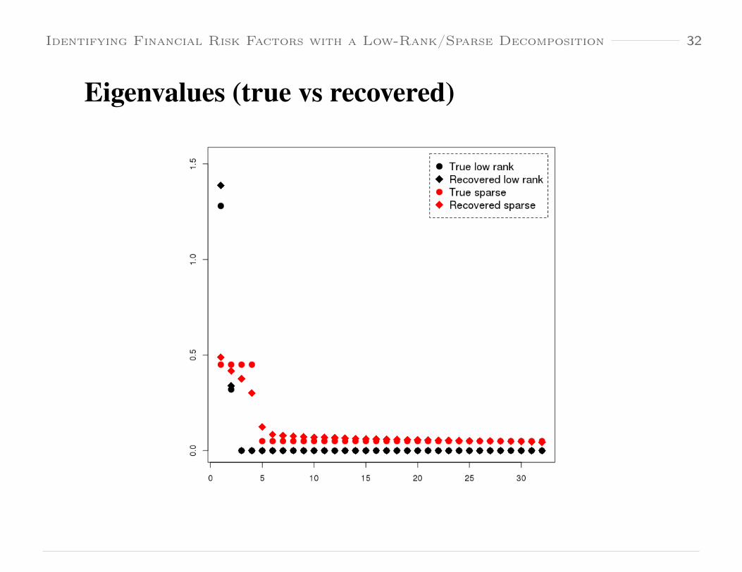
Identifying Financial Risk Factors with a Low-Rank/Sparse Decomposition 32

Eigenvalues (true vs recovered)

Identifying Financial Risk Factors with a Low-Rank/Sparse Decomposition 33

Numerical studies (real data)

• 𝑁 = 32 securities

• 𝑇 = 260 observations (one year of daily data)

• 𝐾 = ? broad factors

• Securities drawn from 𝜅 = 4 countries

– China

– Argentina

– India

– Saudi Arabia

Identifying Financial Risk Factors with a Low-Rank/Sparse Decomposition 34

Algorithm input: sample covariance, Oct. 2015

Identifying Financial Risk Factors with a Low-Rank/Sparse Decomposition 35

LRPS decomposition (covariance)

Identifying Financial Risk Factors with a Low-Rank/Sparse Decomposition 36

Sample correlation matrix, Oct. 2015

Identifying Financial Risk Factors with a Low-Rank/Sparse Decomposition 37

LRPS decomposition (correlations)

Identifying Financial Risk Factors with a Low-Rank/Sparse Decomposition 38

Recovered eigenvalues

Identifying Financial Risk Factors with a Low-Rank/Sparse Decomposition 39

PCA solution (K=4) and remainder

Identifying Financial Risk Factors with a Low-Rank/Sparse Decomposition 40

Questions.(ads2@berkeley.edu)

Identifying Financial Risk Factors with a Low-Rank/Sparse Decomposition 40-1

ReferencesAnderson, TW (Theodore Wilbur) (1968), An introduction to multivariate sta-

tistical analysis, John Wiley & Sons.

Bentler, Peter M & Jeffrey S Tanaka (1983), ‘Problems with em algorithms forml factor analysis’, Psychometrika 48(2), 247–251.

Bickel, Peter J & Elizaveta Levina (2008), ‘Covariance regularization by thresh-olding’, The Annals of Statistics pp. 2577–2604.

Candès, Emmanuel J & Benjamin Recht (2009), ‘Exact matrix completionvia convex optimization’, Foundations of Computational mathematics9(6), 717–772.

Candès, Emmanuel J, Xiaodong Li, Yi Ma & John Wright (2011), ‘Robust prin-cipal component analysis?’, Journal of the ACM (JACM) 58(3), 11.

Chamberlain, Gary & Michael Rothschild (1982), ‘Arbitrage, factor structure,and mean-variance analysis on large asset markets’.

Identifying Financial Risk Factors with a Low-Rank/Sparse Decomposition 40-2

Chandrasekaran, Venkat, Pablo A Parrilo & Alan S Willsky (2010), Latent vari-able graphical model selection via convex optimization, in ‘Communica-tion, Control, and Computing (Allerton), 2010 48th Annual Allerton Con-ference on’, IEEE, pp. 1610–1613.

Chandrasekaran, Venkat, Pablo A Parrilo & Alan S Willsky (2012), ‘Latentvariable graphical model selection via convex optimization’, The Annalsof Statistics 40(4), 1935–1967.

Chandrasekaran, Venkat, Sujay Sanghavi, Pablo A Parrilo & Alan S Will-sky (2011), ‘Rank-sparsity incoherence for matrix decomposition’, SIAMJournal on Optimization 21(2), 572–596.

De La Torre, Fernando & Michael J Black (2003), ‘A framework for robust sub-space learning’, International Journal of Computer Vision 54(1-3), 117–142.

Drton, Mathias, Bernd Sturmfels & Seth Sullivant (2007), ‘Algebraic factoranalysis: tetrads, pentads and beyond’, Probability Theory and RelatedFields 138(3-4), 463–493.

Identifying Financial Risk Factors with a Low-Rank/Sparse Decomposition 40-3

Fischler, Martin A & Robert C Bolles (1981), ‘Random sample consensus: aparadigm for model fitting with applications to image analysis and auto-mated cartography’, Communications of the ACM 24(6), 381–395.

Gnanadesikan, Ramanathan & John R Kettenring (1972), ‘Robust estimates,residuals, and outlier detection with multiresponse data’, Biometricspp. 81–124.

Jolliffe, Ian (2002), Principal component analysis, Wiley Online Library.

Jöreskog, Karl G (1967), ‘A general approach to confirmatory maximum likeli-hood factor analysis’, ETS Research Bulletin Series 1967(2), 183–202.

Karoui, Noureddine El (2008), ‘Spectrum estimation for large dimensional co-variance matrices using random matrix theory’, The Annals of Statisticspp. 2757–2790.

Ke, Qifa & Takeo Kanade (2005), Robust l 1 norm factorization in the presenceof outliers and missing data by alternative convex programming, in ‘Com-puter Vision and Pattern Recognition, 2005. CVPR 2005. IEEE ComputerSociety Conference on’, Vol. 1, IEEE, pp. 739–746.

Identifying Financial Risk Factors with a Low-Rank/Sparse Decomposition 40-4

Ma, Shiqian, Lingzhou Xue & Hui Zou (2013), ‘Alternating direction methodsfor latent variable gaussian graphical model selection’, Neural computa-tion 25(8), 2172–2198.

Petersen, Kaare Brandt & Michael Syskind Pedersen (2008), ‘The matrix cook-book’, Technical University of Denmark 7, 15.

Rosenberg, Barr (1984), ‘Prediction of common stock investment risk’, TheJournal of Portfolio Management 11(1), 44–53.

Ross, Stephen A (1976), ‘The arbitrage theory of capital asset pricing’, Journalof economic theory 13(3), 341–360.

Rubin, Donald B & Dorothy T Thayer (1982), ‘Em algorithms for ml factoranalysis’, Psychometrika 47(1), 69–76.

Rubin, Donald B & Dorothy T Thayer (1983), ‘More on em for ml factor anal-ysis’, Psychometrika 48(2), 253–257.

Saunderson, James, Venkat Chandrasekaran, Pablo A Parrilo & Alan S Will-sky (2012), ‘Diagonal and low-rank matrix decompositions, correlation

Identifying Financial Risk Factors with a Low-Rank/Sparse Decomposition 40-5

matrices, and ellipsoid fitting’, SIAM Journal on Matrix Analysis and Ap-plications 33(4), 1395–1416.

Shapiro, Alexander (1982), ‘Rank-reducibility of a symmetric matrix and sam-pling theory of minimum trace factor analysis’, Psychometrika 47(2), 187–199.

Shapiro, Alexander (1985), ‘Identifiability of factor analysis: Some results andopen problems’, Linear Algebra and its Applications 70, 1–7.

Shapiro, Alexander & Jos MF Ten Berge (2002), ‘Statistical inference of mini-mum rank factor analysis’, Psychometrika 67(1), 79–94.

Sharpe, William F (1964), ‘Capital asset prices: A theory of market equilibriumunder conditions of risk’, The journal of finance 19(3), 425–442.

Treynor, Jack L (1962), Toward a theory of market value of risky assets. Pre-sented to the MIT Finance Faculty Seminar.

Wilson, Edwin B & Jane Worcester (1939), ‘The resolution of six tests intothree general factors’, Proceedings of the National Academy of Sciencesof the United States of America 25(2), 73.