Hypothesis TestingDavid YoungDepartment of Statistics and Modelling Science, University of StrathclydeRoyal Hospital for Sick Children, Yorkhill NHS Trust

Statistics and Probability•statistical analysis considers the probability of an event being

due to chance•can never be 100% certain for example that one treatment is

better than another•can say mathematically how sure we are that a result is true

2

Hypothesis Testing•a statistical tests is designed to ‘prove’ a hypothesis held by the

researcher•it starts by assuming the contrary view to the researcher’s and

only comes down in support of the researcher’s hypothesis if the data are sufficiently unlikely to have been generated by the contrary view

•the ‘contrary view’ is known as the null hypothesis•the research hypothesis of interest is called the alternative

hypothesis

3

Probability•in statistical testing, it is impossible to ‘prove’ a hypothesis

beyond all reasonable doubt•decision processes must be able to deal with the problems of

uncertainty•modelling of uncertainty is impossible with standard

mathematical tools and a whole branch of mathematics called Probability Theory has been developed to deal with it

•most people have a good grasp of probability through card games, board games, betting odds, etc.

4

Probability Theory•suppose that the proportion (p) of defective items in a large

batch is 0.1•in a sample size 100 taken from this batch, we would expect to

get (1000.1)=10 defective items•a single sample may contain any number of defective items

‘close’ to 10•e.g. samples may have 8, 11, 9, 10 or 12 defectives•probability theory enables us to calculate the probability or

chance of getting a given number of defectives

5

Hypothesis Testing•statistical inference is the procedure whereby inferences about

a population are made on the basis of the results obtained from a sample drawn from that population

•inference may be divided into two categories …• estimation• hypothesis testing

•basically, hypothesis testing is a test of the validity of some claim or theory about a population e.g. students have debts of >£4000 upon graduating, aspirin is a more effective pain-killer than paracetamol, a new HIV medication delays the onset of AIDS, etc.

6

Comparing Two Samples of Data•there are several factors which affect the choice of statistical

hypothesis test• in comparing two sample means the procedure depends on

whether the data are paired (as in a cross-over experiment of when comparing a ‘before’ and ‘after’ measurements)

•whether the data are quantitative or qualitative•it also depends on the distribution of the sample data (are the

data normal?)

7

Checking the Assumption of Normality•the simplest way to check the normality assumption for a

variable is by plotting a histogram and assessing visually if the distribution is bell-shaped

•normality tests are available with most statistical packages•e.g. in MINITAB the normality test generates a normal

probability plot and performs a hypothesis test to examine whether or not the observations follow a normal distribution

•for data which are normally distributed, parametric tests can be applied

8

Distribution Free Tests•occasionally it will not be possible to make this assumption e.g.

when the data are clearly skewed or there are too few data points to determine the approximate distribution

•a group of tests have been devised for which no assumptions are made about the distribution of the observations – these are called distribution-free tests

•since distributions are compared without the use of parameters they can be referred to as non-parametric tests

9

Comparing Unpaired Samples• in a sense we wish to compare the ‘average’ values for the two

underlying populations e.g. does the average blood pressure differ in two groups treated with a different drug?• if the samples are normally distributed, use a t-test and the

corresponding confidence intervals to compare the means

10

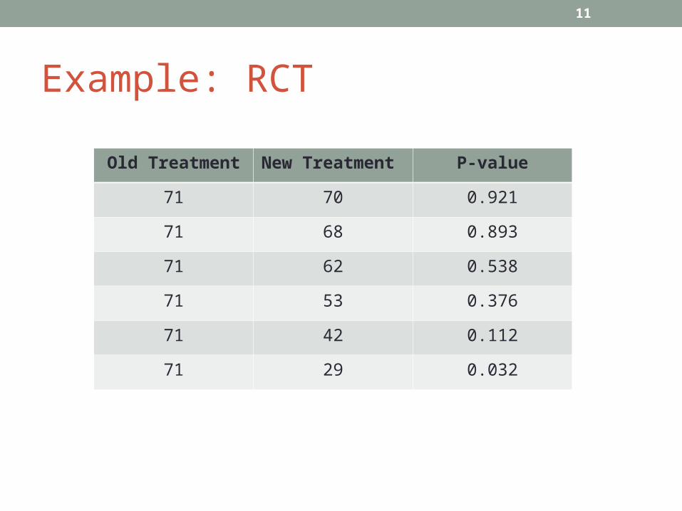
Example: RCT

Old Treatment New Treatment P-value

71 70 0.921

71 68 0.893

71 62 0.538

71 53 0.376

71 42 0.112

71 29 0.032

11

Additional Points•Errors in hypothesis testing – p<0.01!•Null and alternative hypotheses•Cranberry juice – randomisation

http://www.ncbi.nlm.nih.gov/pubmed/22961092

12

Additional Points•Double blind studieshttp://www.theguardian.com/society/2005/jan/17/

health.medicineandhealth

•Placebo trials•Comparison of baseline characteristics•Intention-to-treat and per-protocol – weight loss example•Tests for correlation, regression and normality testing

13

Example•Comparison of transit times (hours) using two different bran

preparations ...http://www.ncbi.nlm.nih.gov/pmc/articles/PMC1410956/•Bran preparation A:

44 51 52 55 60 62 66 68 69 71 71 76 82 91 108•Bran preparation B:

52 64 68 77 79 83 84 88 95 97 101 116•null hypothesis – no difference in transit times for A and B•alternative hypothesis – some difference in transit times

14

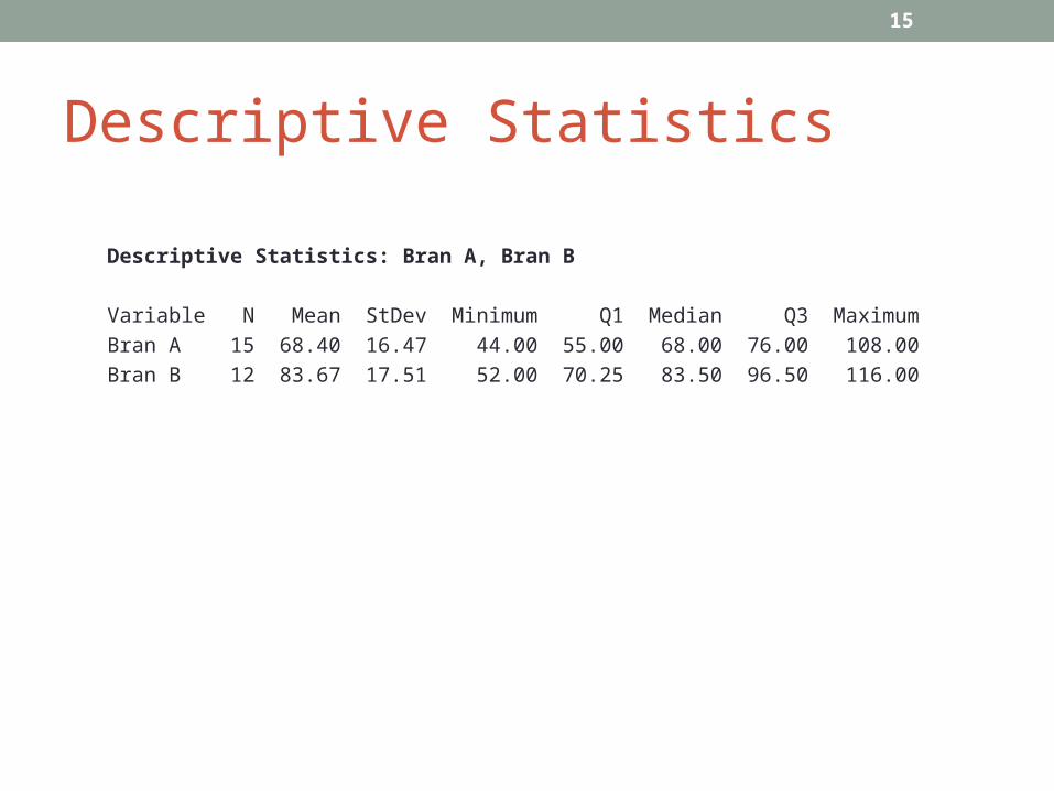
Descriptive Statistics

Descriptive Statistics: Bran A, Bran B

Variable N Mean StDev Minimum Q1 Median Q3 Maximum

Bran A 15 68.40 16.47 44.00 55.00 68.00 76.00 108.00

Bran B 12 83.67 17.51 52.00 70.25 83.50 96.50 116.00

15

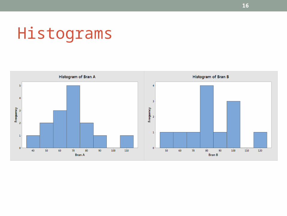
Histograms

16

The P-value•the p-value is the probability of getting data as extreme as

those actually observed in the experiment if the null hypothesis were true

•the lower the p-value, the more evidence there is against the null hypothesis (i.e. in favour of the study hypothesis)

•the conventional cut-off for significance is p<0.05

17

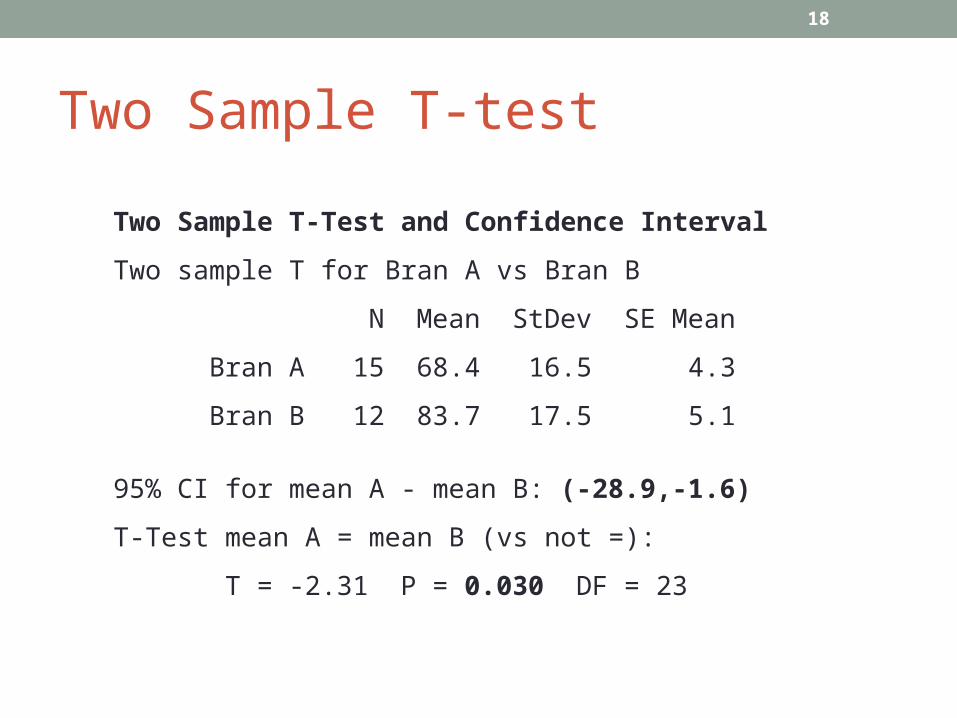
Two Sample T-test

Two Sample T-Test and Confidence Interval

Two sample T for Bran A vs Bran B

N Mean StDev SE Mean

Bran A 15 68.4 16.5 4.3

Bran B 12 83.7 17.5 5.1

95% CI for mean A - mean B: (-28.9,-1.6)

T-Test mean A = mean B (vs not =):

T = -2.31 P = 0.030 DF = 23

18

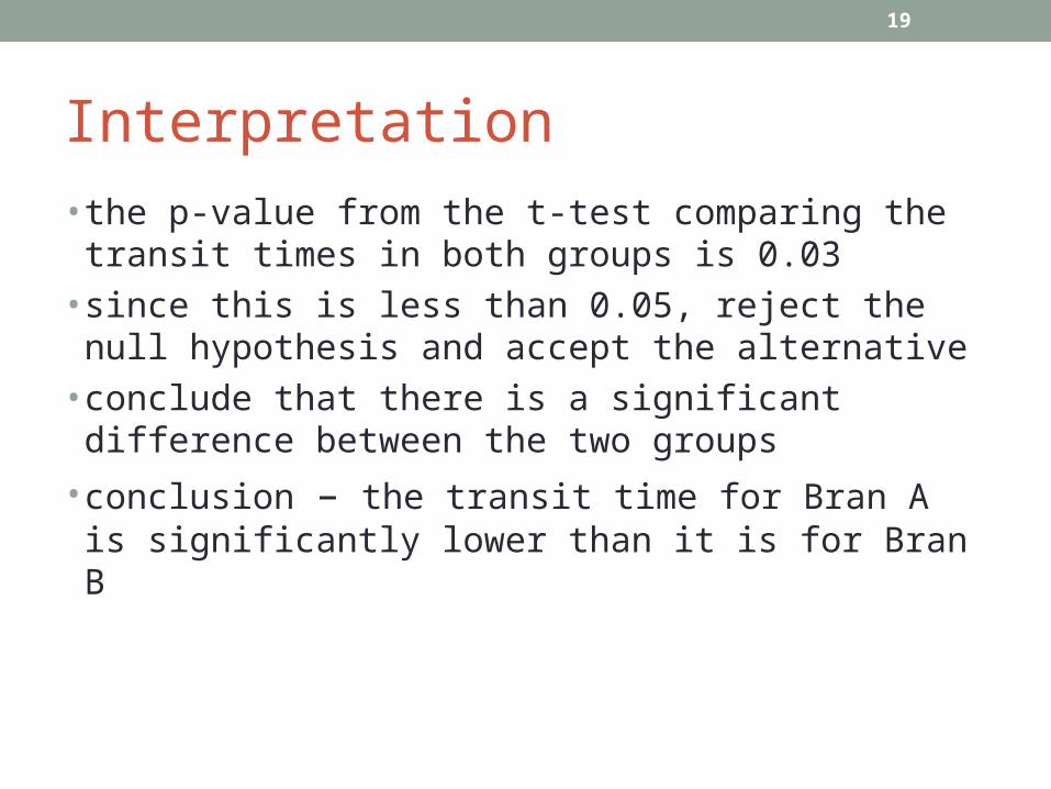
Interpretation•the p-value from the t-test comparing the transit times in both

groups is 0.03•since this is less than 0.05, reject the null hypothesis and

accept the alternative•conclude that there is a significant difference between the two

groups•conclusion – the transit time for Bran A is significantly lower

than it is for Bran B

19

Choice of Test•the choice of statistical test to use depends mainly on two

things …– the type of data (categorical or numerical)– the distribution of the data (normal or non-normal)

•if the data are normally distributed, parametric tests are used•if the data are not normally distributed, non-parametric tests

are appropriate

20

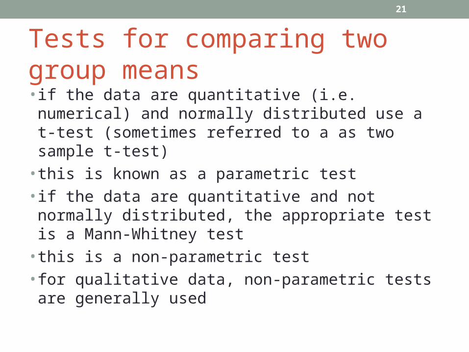
Tests for comparing two group means•if the data are quantitative (i.e. numerical) and normally

distributed use a t-test (sometimes referred to a as two sample t-test)

•this is known as a parametric test• if the data are quantitative and not normally distributed, the

appropriate test is a Mann-Whitney test•this is a non-parametric test•for qualitative data, non-parametric tests are generally used

21

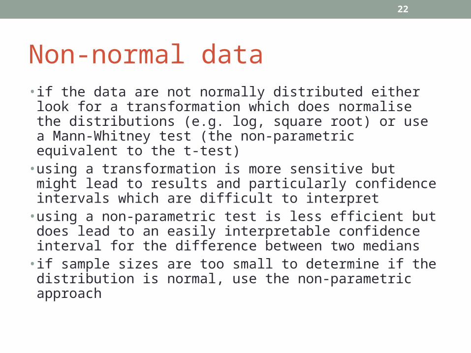
Non-normal data•if the data are not normally distributed either look for a

transformation which does normalise the distributions (e.g. log, square root) or use a Mann-Whitney test (the non-parametric equivalent to the t-test)

•using a transformation is more sensitive but might lead to results and particularly confidence intervals which are difficult to interpret

•using a non-parametric test is less efficient but does lead to an easily interpretable confidence interval for the difference between two medians

•if sample sizes are too small to determine if the distribution is normal, use the non-parametric approach

22

Qualitative Data•this involves comparing the proportion of cases who have a

certain characteristic of interest in the two groups e.g. do the proportions of cases suffering from a breast cancer recurrence differ for pre and post-menopausal women?

•with decent sample sizes use a chi-squared test along with a confidence interval for the difference or ratio of the two proportions

23

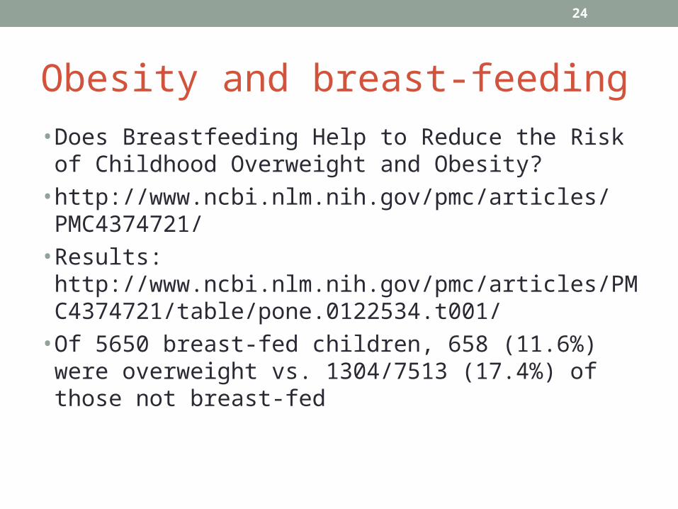
Obesity and breast-feeding• Does Breastfeeding Help to Reduce the Risk of Childhood

Overweight and Obesity?• http://www.ncbi.nlm.nih.gov/pmc/articles/PMC4374721/• Results:

http://www.ncbi.nlm.nih.gov/pmc/articles/PMC4374721/table/pone.0122534.t001/• Of 5650 breast-fed children, 658 (11.6%) were overweight vs.

1304/7513 (17.4%) of those not breast-fed

24

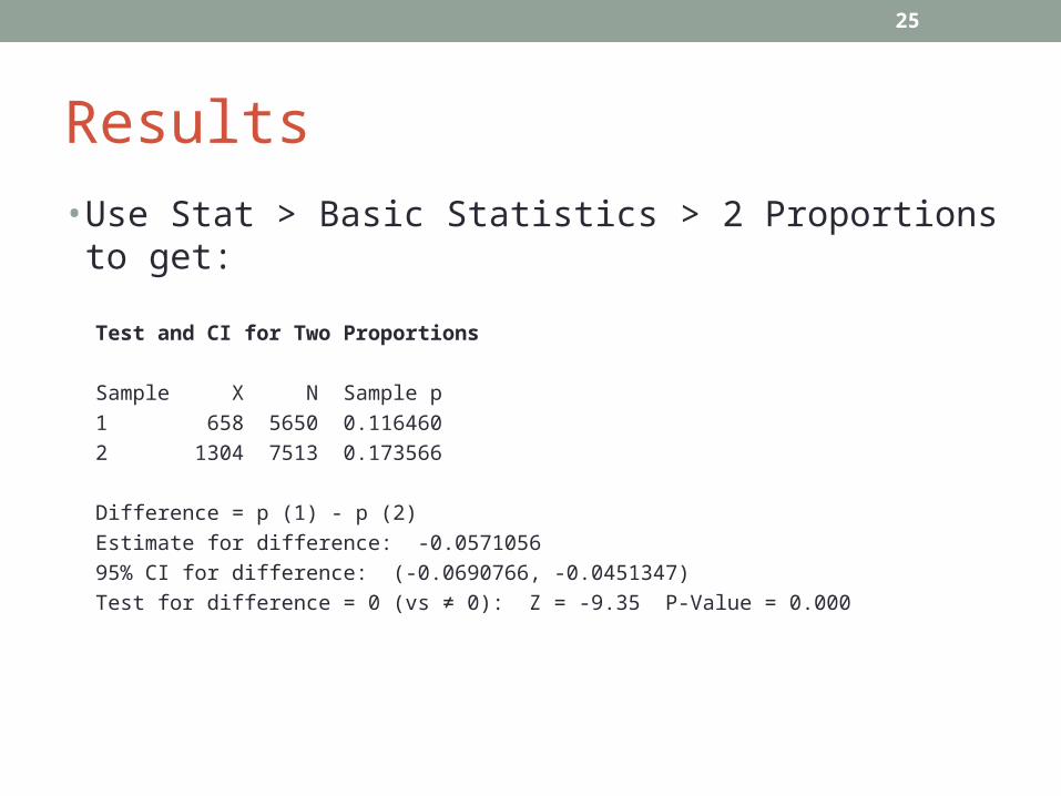
Results•Use Stat > Basic Statistics > 2 Proportions to get:

Test and CI for Two Proportions

Sample X N Sample p

1 658 5650 0.116460

2 1304 7513 0.173566

Difference = p (1) - p (2)

Estimate for difference: -0.0571056

95% CI for difference: (-0.0690766, -0.0451347)

Test for difference = 0 (vs ≠ 0): Z = -9.35 P-Value = 0.000

25

Comparing Paired Samples•the same issues must be addressed when deciding upon the

analysis method for a given set of paired data•problem types are essentially the same only in this case the

same individual has been measured twice•before we made assumptions about the distributions in the

separate groups whereas here the assumptions relate to the within individual differences

26

Quantitative Data•if the differences between the two samples follow a normal

distribution (possibly after transformation) then use a paired t-test and compute a confidence interval to compare the two means

•if the differences are not normal then use a Wilcoxon signed rank test (the non-parametric equivalent of the paired t-test)

27

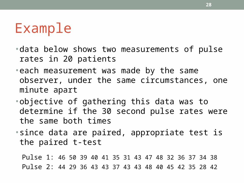
Example•data below shows two measurements of pulse rates in 20

patients•each measurement was made by the same observer, under the

same circumstances, one minute apart•objective of gathering this data was to determine if the 30

second pulse rates were the same both times•since data are paired, appropriate test is the paired t-test

Pulse 1: 46 50 39 40 41 35 31 43 47 48 32 36 37 34 38Pulse 2: 44 29 36 43 43 37 43 43 48 40 45 42 35 28 42

28

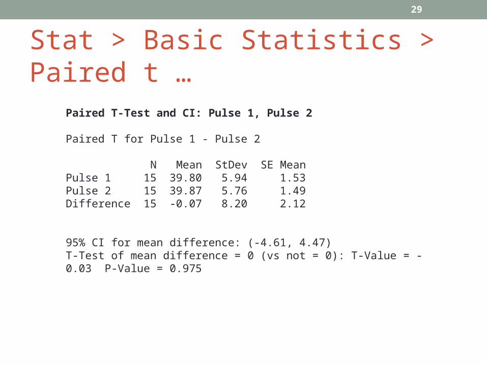
Stat > Basic Statistics > Paired t …Paired T-Test and CI: Pulse 1, Pulse 2

Paired T for Pulse 1 - Pulse 2

N Mean StDev SE MeanPulse 1 15 39.80 5.94 1.53Pulse 2 15 39.87 5.76 1.49Difference 15 -0.07 8.20 2.12

95% CI for mean difference: (-4.61, 4.47)T-Test of mean difference = 0 (vs not = 0): T-Value = -0.03 P-Value = 0.975

29

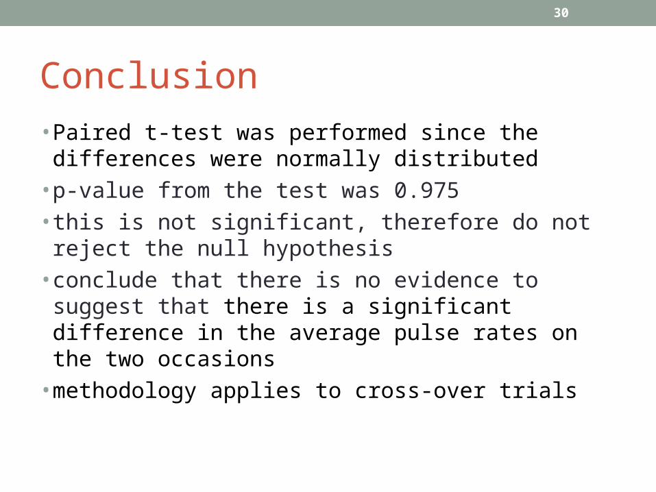
Conclusion•Paired t-test was performed since the differences were

normally distributed•p-value from the test was 0.975•this is not significant, therefore do not reject the null

hypothesis•conclude that there is no evidence to suggest that there is a

significant difference in the average pulse rates on the two occasions

•methodology applies to cross-over trials

30

Summary•the set-up for a hypothesis test is always the same …•determine the null and alternative hypotheses•choose the appropriate test based on the type and distribution

of the data•if the p-value is less than 0.05, reject the null hypothesis and

conclude that there is evidence to support the alternative hypothesis

• if the p-value is not significant (i.e. >0.05), conclude there is no evidence to reject the null hypothesis

31

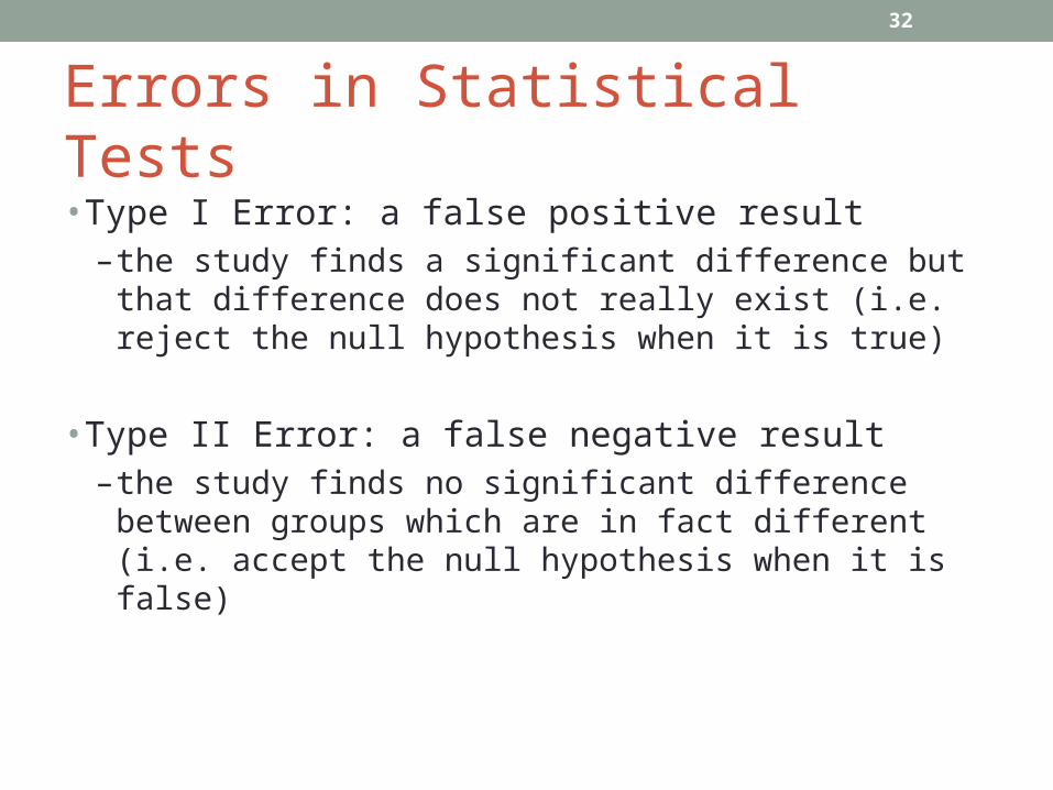
Errors in Statistical Tests•Type I Error: a false positive result

– the study finds a significant difference but that difference does not really exist (i.e. reject the null hypothesis when it is true)

•Type II Error: a false negative result– the study finds no significant difference between groups which are

in fact different (i.e. accept the null hypothesis when it is false)

32

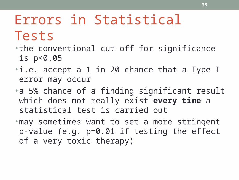
Errors in Statistical Tests•the conventional cut-off for significance is p<0.05•i.e. accept a 1 in 20 chance that a Type I error may occur•a 5% chance of a finding significant result which does not really

exist every time a statistical test is carried out•may sometimes want to set a more stringent p-value (e.g.

p=0.01 if testing the effect of a very toxic therapy)

33

Confidence Intervals•the sample mean is only an estimate of the population mean•estimates depend on the sample from which they are

calculated•a range of plausible values of the mean can be computed•this gives an interval in which we can be relatively sure the true

population parameter value lies•these intervals are known as confidence intervals

34

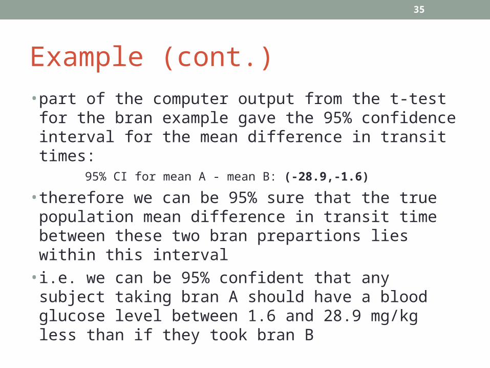
Example (cont.)•part of the computer output from the t-test for the bran

example gave the 95% confidence interval for the mean difference in transit times:

95% CI for mean A - mean B: (-28.9,-1.6)

•therefore we can be 95% sure that the true population mean difference in transit time between these two bran prepartions lies within this interval

• i.e. we can be 95% confident that any subject taking bran A should have a blood glucose level between 1.6 and 28.9 mg/kg less than if they took bran B

35

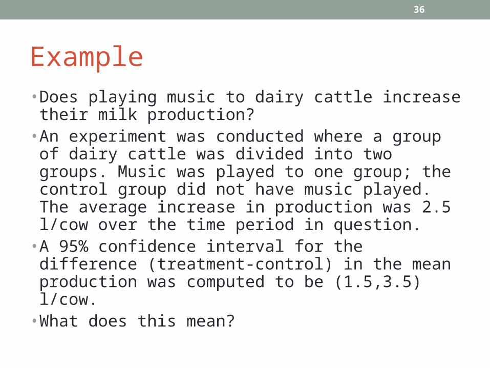
Example•Does playing music to dairy cattle increase their milk

production? •An experiment was conducted where a group of dairy cattle

was divided into two groups. Music was played to one group; the control group did not have music played. The average increase in production was 2.5 l/cow over the time period in question.

•A 95% confidence interval for the difference (treatment-control) in the mean production was computed to be (1.5,3.5) l/cow.

•What does this mean?

36