Embed Size (px)
Citation preview

Hypercomputation: computing more than the Turing machine
Toby OrdDepartment of Philosophy*
The University of [email protected]
Abstract:
In this report I provide an introduction to the burgeoning field of hypercomputation – the study ofmachines that can compute more than Turing machines. I take an extensive survey of many of the keyconcepts in the field, tying together the disparate ideas and presenting them in a structure whichallows comparisons of the many approaches and results. To this I add several new results and drawout some interesting consequences of hypercomputation for several different disciplines.
I begin with a succinct introduction to the classical theory of computation and its place amongst someof the negative results of the 20th Century. I then explain how the Church-Turing Thesis is commonlymisunderstood and present new theses which better describe the possible limits on computability.Following this, I introduce ten different hypermachines (including three of my own) and discuss insome depth the manners in which they attain their power and the physical plausibility of eachmethod. I then compare the powers of the different models using a device from recursion theory.
Finally, I examine the implications of hypercomputation to mathematics, physics, computer scienceand philosophy. Perhaps the most important of these implications is that the negative mathematicalresults of Gödel, Turing and Chaitin are each dependent upon the nature of physics. This bothweakens these results and provides strong links between mathematics and physics. I conclude thathypercomputation is of serious academic interest within many disciplines, opening new possibilitiesthat were previously ignored because of long held misconceptions about the limits of computation.
* The majority of this report was written as an Honours thesis at the Department of Computer Science in the University ofMelbourne. This work was supervised by Harald Søndergaard.

Acknowledgments
In writing this report, I am indebted to four people. Jack Copeland, for introducing me tohypercomputation and taking my new ideas seriously. Harald Søndergaard, for allowing me thechance to do my Honours thesis on such a fascinating topic and then keeping me focused when Iinevitably tried to take on too much. Peter Eckersley, for his ever enthusiastic conversations on thelimits of logical thought. And finally, Bernadette Young, for her kindness and support when thingslooked impossible.

Preface
It has long been assumed that the Turing machine computes all the functions that are computable inany reasonable sense. It is therefore assumed to be a sufficient model for computability. What then, isone to make of the slow trickle of papers that discuss models which can compute more than theTuring machine? It is perhaps tempting to dismiss such theorising as idle speculation alike to the morefanciful areas of pure mathematics, in which models and abstractions are studied for their own sakewith little regard to any real world implications.
This would be a great mistake. The study of more powerful models of computation is of considerableimportance, with many far-reaching implications in computer science, mathematics, physics andphilosophy. Rarely, if ever, has such an important physical claim about the limits of the universe beenso widely accepted from such a weak basis of evidence. The inability of some of the best minds of thecentury to develop ways in which we could build machines with more computational power thanTuring machines is not good evidence that this is impossible. At best, it is reason to consider theproblem to be very difficult and likely to require a radically new technique or even new developmentsin physics.
However, we should not even go this far. A variety of theoretical models for such hypercomputation havebeen presented over the past century. They have, however, often been presented in rather theoreticalcontexts, which explains the lack of serious work on exploring the physical realisability of thesemodels. Indeed, from what work has been done, there have recently been several serious reports abouthow quantum mechanics and relativity may be used to harness hypercomputation.
In many ways, the present theory of computation is in a similar position to that of geometry in the 18th
and 19th Centuries. In 1817 one of the most eminent mathematicians, Carl Friedrich Gauss, becameconvinced that the fifth of Euclid’s axioms was independent of the other four and not self evident, sohe began to study the consequences of dropping it. However, even Gauss was too fearful of thereactions of the rest of the mathematical community to publish this result. Eight years later, JánosBolyai published his independent work on the study of geometry without Euclid’s fifth axiom andgenerated a storm of controversy to last many years.
His work was considered to be in obvious breach of the real-world geometry that the mathematicssought to model and thus an unnecessary and fanciful exercise. However, the new generalisedgeometry (of which Euclidean geometry is but a special case) gathered a following and led to manynew ideas and results. In 1915, Einstein’s general theory of relativity suggested that the geometry ofour universe is indeed non-Euclidean and was supported by much experimental evidence. The non-

Euclidean geometry of our universe must now be taken into account in both the calculations oftheoretical physics and those of a taxi’s global positioning system.
Until now, much of the work on hypercomputation has been independently derived, with theoccasional new models discussed in relative isolation with only a brief look at their implications. In thisreport I try to somewhat remedy this situation, presenting a survey of much of the past work onhypercomputation. I explain many of the models that have been presented and analyse theirrequirements and capabilities before drawing out the considerable implications that they bear formany important areas of mathematics and science.

Contents
1 Introduction – Classical Computation ............................................................................. 11.1 Gödel's Incompleteness Theorem...............................................................................................11.2 Turing Machines and Computation...........................................................................................21.3 Turing Machines and Semi-computation...................................................................................51.4 Algorithmic Information Theory ................................................................................................7
2 Hypercomputation ..........................................................................................................102.1 The Church-Turing Thesis .......................................................................................................102.2 Other Relevant Theses..............................................................................................................112.3 Recursion Theory......................................................................................................................142.4 A Note on Terminology ............................................................................................................15
3 Hypermachines ...............................................................................................................163.1 O-Machines ...............................................................................................................................163.2 Turing Machines with Initial Inscriptions ................................................................................173.3 Coupled Turing Machines ........................................................................................................173.4 Asynchronous Networks of Turing Machines ..........................................................................183.5 Error Prone Turing Machines ..................................................................................................183.6 Probabilistic Turing Machines..................................................................................................183.7 Infinite State Turing Machines .................................................................................................193.8 Accelerated Turing Machines...................................................................................................203.9 Infinite Time Turing Machines ................................................................................................203.10 Fair Non-Deterministic Turing Machines................................................................................22
4 Resources ........................................................................................................................234.1 Assessing the Resources Used to Achieve Hypercomputation ................................................234.2 Infinite Memory.........................................................................................................................244.3 Non-Recursive Information Sources ........................................................................................254.4 Infinite Specification..................................................................................................................284.5 Infinite Computation.................................................................................................................284.6 Fair Non-Determinism ..............................................................................................................31
5 Capabilities .....................................................................................................................325.1 The Arithmetical Hierarchy......................................................................................................325.2 Comparative Powers..................................................................................................................33

6 Implications ....................................................................................................................376.1 To Mathematics.........................................................................................................................376.2 To Physics ..................................................................................................................................396.3 To Computer Science ...............................................................................................................406.4 To Philosophy............................................................................................................................42
7 Conclusions and Further Work .......................................................................................437.1 Conclusions................................................................................................................................437.2 Further Work .............................................................................................................................44
References...........................................................................................................................46
Appendix.............................................................................................................................49

1
Chapter 1
Introduction – Classical Computation
1.1 Gödel's Incompleteness Theorem
The desire to capture the complexities of mathematical reasoning and computation in a simple andpowerful manner has been a major theme of 20th Century mathematics. While developing these ideas,several powerful negative results were reached about the limitations of computation. I refer here to theresults of Kurt Gödel, Alan Turing and Gregory Chaitin. Each of these built upon the last to reachmore powerful conclusions about the limitations of mathematical knowledge. As well as providing aframework for the rest of this report, these ideas will hopefully be clarified by material in later chaptersand will be shown in a new and more positive light.
The 1930’s saw two of these great negative results in the foundations of mathematics, the first of whichwas Gödel’s very unexpected proof of 1931. In arguably the most important mathematical paper ofthe 20th Century [27], he proved that the leading formalisation of mathematics, Principia Mathematica,was either an incomplete or inconsistent theory of the natural numbers. In other words, that there arepropositions in the language of arithmetic that are either true but unprovable within PrincipiaMathematica or false but provable. Since consistency is required of all serious proof systems, Gödel'sresult is considered a proof of the incompleteness of Principia Mathematica and is known as Gödel'sIncompleteness Theorem.
He proved the incompleteness of Principia Mathematica with a combination of two insightful ideas.First, he showed how formulae could be associated with natural numbers, to allow statements inarithmetic to refer to other statements in arithmetic. Then he showed how the predicate 'is provable inPrincipia Mathematica' could be translated into a statement in arithmetic. This allowed him toconstruct a statement that says of itself that it is not provable within Principia Mathematica. Thisstatement has the desired property of being either true but unprovable or false but provable.
The existence of such statements for Principia Mathematica would have been considered a majorresult in itself, but Gödel went further and argued that his method of proof could be applied to anyformal proof system that operates be finite means. In other words, that all mechanical methods fordescribing a set of axioms and the rules by which theorems can be inferred can be translated intostatements in arithmetic. From these statements, one could then construct new statements that attestto their own unprovability. As a consequence every such system would be incomplete.
2
This claim that no consistent formal system can prove all truths of arithmetic was seen as a profoundlynegative result for mathematics. While on the surface it is only a limitation for our formalisationprocesses (and Gödel himself believed that it was not a limitation for human reasoning [21]), it wastaken by many to show that there are statements in arithmetic whose truth is unknowable. Gödel’sIncompleteness Theorem is thus usually considered to be a major limitation on the power ofreasoning.
1.2 Turing Machines and Computation
The second great breakthrough is intimately related to the first – completing it and extending it.Although Gödel's argument was generally accepted by the mathematical community as showing theincompleteness of all formal proof systems, it relied upon the intuitive notion of a generalised formalsystem. While the proof of the incompleteness of Principia Mathematica was finished andunquestionable, the incompleteness of all formal systems was dependent upon a concreteinterpretation of a 'mechanical method' or 'finite means'.
The formal analysis of computation by finite means was also motivated by other problems of the day.The Entscheidungsproblem1 and Hilbert’s tenth problem2 both asked for algorithms to solve importantmathematical problems. The failure of past efforts to find these algorithms had made somemathematicians suspect that there were, in fact, no algorithms to solve them. Proving the absence of amechanical method for doing something required a precise formalisation of what mechanicalcomputation is. 1936 saw the independent development of three influential models of computation,aimed at doing just this: the lambda calculus, recursive functions and Turing machines.
All three were soon found to agree on which functions were computable, differing only in how theywere to be computed. Alonzo Church’s lambda calculus [11] and Steven Kleene’s recursive functions[33] were arguably more elegant in this respect, but it was the mechanical action of Turing’s machines[52] that most agreed with intuitions about how people go about computing mathematical functions.Unlike the others, it was as much an instruction manual on how such a device might be built as it wasa formalism for studying computation. This link between abstract computability and physicalcomputability made Turing machines quickly become the standard model of computation. It alsomakes Turing machines a natural object for studying even more powerful models of computation, asis done later in this report.
A Turing machine consists of two main parts: a 'tape' for storing the input, output and scratchworking, and a set of internal states and transitions detailing how the machine should function.
The tape is made up of an infinite sequence of squares, each of which can have one symbol written onit. It is usually considered as a long strip of paper that is bounded on the left, but stretches infinitely tothe right. While this infinite length of the tape may seem quite unrealistic, it is normally justified byconsidering it to be finite but unbounded – we can imagine that the machine begins with a finitesequence of squares and new blank squares are produced and added to the tape as needed.
1 The problem of deciding whether an arbitrary formula of the predicate calculus is a tautology.
2 The problem of solving an arbitrary diophantine equation (a polynomial equation with integer variables).

3
The tape begins with the input inscribed upon it and then, as the computation progresses, this getsgradually altered until it eventually contains just the output. The symbols that can be inscribed on thetape come from a fixed and finite alphabet, S, and each square can hold one symbol. Initially a finitesequence of symbols is placed upon the tape and the rest is left blank. While we could use quitecomplicated alphabets, we will usually use an alphabet consisting of just two symbols: 0 and 1. Weequate 0 with the blank square and assume the tape to begin with a finite quantity of 1’s placed atfinite distances from the beginning of the tape and the rest is filled with 0’s.
This tape is linked to the operation of the machine through a 'tape head' which, at any time, isconsidered to be looking at one particular square of the tape. The instructions of the machine canmake this tape head scan the current symbol, change the symbol, move to the left or move to theright.
When the machine is started, it begins in a specified 'initial state'. Associated with this state are a finitelist of instructions each of which has four parts (symbol 1, symbol 2, direction, new state). The machinetreats this instruction as follows: if symbol 1 is at the tape head then replace it by symbol 2, move thetape head in the specified direction and then follow the instructions in the new state. If an instruction isnot applicable (i.e. symbol 1 is not under the tape head) then it tries the next instruction. At most oneinstruction can be applicable at a given time and thus there can only be as many instructions for agiven state as there are symbols. If no instructions are applicable, the machine halts and thecomputation is over, with the output being whatever is written on the tape at that time. If a givencomputation does not halt, it is said to diverge and does not produce any output.
While computation here has been defined over functions from finite strings in S to finite strings in S, itis also possible to consider the computation of other types of functions. For now, I will only examinefunctions from natural numbers to natural numbers. I will represent the number n in unary as a 0followed by n 1's (followed by an infinite sequence of 0’s).
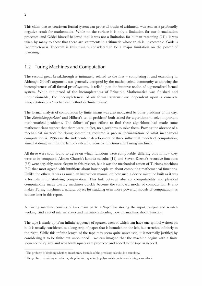
The following is a short program to demonstrate this idea. It simply takes a representation of a naturalnumber and returns 1 if it is even and 0 if it is not. Figure 1 is represents this Turing machinegraphically.
state 0: ( 0, 0, right, 1 )
state 1: ( 1, 1, right, 1)( 0, 0, left, 2)
state 2: ( 1, 0, left, 3)( 0, 0, right, 4)
state 3: ( 1, 0, left, 2)
state 4: ( 0, 1, left, 6 )
state 5: [no instructions] Figure 1

4
initial tape: initial tape:
final tape: final tape:
To represent a real number (between 0 and 1) we can use an infinite sequence over {0, 1} to representthe digits of the real in binary3. Although a computation that generates such a sequence never finishes,there is a sense in which the real is being computed: if we want to know the value of the real to n bitsof accuracy, we can wait until the Turing machine produces the first n bits.
There is a slight catch however, which is that when computing a complicated real such as p, we needsome way of knowing which digits are finalised and which are not. To do this, we can give themachine another symbol # such that it prints # between every two bits of the real and never altersanything to the left of a #4.
For example, this Turing machine (starting with a blank tape) computes the value of 1§3 in binary:
state 0: ( 0, 0, right, 1 )
state 1: ( 0, #, right, 2 )
state 2: ( 0, 1, right, 3 )
state 3: ( 0, #, right, 0 )
initial tape:
final tape:
An infinite set of natural numbers can be represented by a real whose (n+1)th digit is 1 if n is in the setand 0 otherwise. A set of natural numbers is computable if and only if its corresponding real iscomputable. Using this encoding, the previous Turing machine computes the set of odd naturals.
While they seem quite simple, Turing machines are able to compute many different functions. Indeed,Turing machines were shown to be able to compute anything that the other proposed models couldcompute and vice versa. Each model was shown to be able to compute the same set of functions andthese functions seemed to be equivalent to those that a mathematician could compute without the useof insight.
Many independent models of computation have been produced which also compute the samefunctions as a Turing machine. Indeed, considerable work has been done on adding extensions to
3 There is no significant problem in representing arbitrary reals, but the arguments are much more clear and concise ifattention is restricted to reals between 0 and 1.
4 Another prominent method for addressing this issue is to give the machine multiple tapes, in particular a read-only inputtape, a standard tape for scratch working and a write-only tape for output. These methods are equivalent.
Figure 2

5
Turing machines – such as allowing them to operate non-deterministically or giving them multipletapes with their own tape heads – but the enhanced models still computed the same functions. Thislent further importance to this set of functions which have come to be known as the (partial) recursivefunctions and even the computable functions.
1.3 Turing Machines and Semi-computation
It was, however, known since the inception of Turing machines that there were functions that theycould not compute. This is clear when you consider that the set of functions from N to N isuncountable while the set of Turing machines is countable. Both Turing and Church went beyondthis however, and showed specific examples of functions which could not be computed [52, 11]. Themost famous of these is Turing’s halting function which takes a natural number representing a Turingmachine and its input, returning 1 if the machine halts on its input and 0 if it does not. From this, wealso get the existence of a specific uncomputable set {n | n represents a Turing machine / input pairthat halts} and an uncomputable real (the nth digit of which is 1 if n represents a Turing machine /input pair that halts and 0 otherwise). This set is known as the halting set and the real number as t, forTuring's constant5.
The halting function can be shown to be uncomputable by Turing machines through a reductioargument. Assuming there is a Turing machine for the halting function, H , we can construct amodified machine H1 which takes an encoding of a Turing machine and determines whether thismachine halts when given its own encoding as input. Now consider another machine H2 which is likeH1, but loops if the given machine halts on its own encoding and halts if the given machine loops onits encoding. If H2 is given an encoding of itself as input, it loops if and only if it would halt. This is acontradiction. Since all other claims are verifiable, our assumption of the existence of H must be inerror.
While the halting function may not be computable by Turing machines in the terms definedpreviously, there is still a sense in which it is partially computable. We can construct a Turingmachine, H’, that takes a representation of a Turing machine, M, with some input, I, and simulatesthe behaviour of M on I. If M does not halt, then H’ does not halt either. If M halts, then H’ also halts,but instead of outputting the result of M on I it just outputs the number 1. Thus, H’ computes thehalting function correctly if the value of the function is 1 and diverges otherwise. It is said that H’ semi-computes the halting function.
In general, we can say a function, f : X -> {0, 1} is semi-computable by Turing machines if there is aTuring machine which transforms input, x, to f(x) whenever f(x) = 1 and either returns 0 or divergeswhen f(x) = 0. Such functions are also said to be recursively enumerable.
Thus, the halting function is semi-computable by Turing machines.
5 There are many trivial 1-1 mappings from the set of Turing Machine / input pairs to the set of natural numbers, and forthese purposes it does not matter which one is used. The different mappings give different halting functions (and different t‘s)but these all have the same important properties.

6
We also say that a function, f : X -> {0, 1} is co-semi-computable by Turing machines if there is a Turingmachine which transforms input, x, to f(x) whenever f(x) = 0 and either returns 1 or diverges whenf(x) = 1. Such functions are also said to be co-recursively enumerable.
Thus the looping function (does a given Turing machine not halt on a given input) is co-semi-computable by Turing machines.
This concept of semi-computability also applies to Turing machines which compute sets or reals. Forreals, being semi-computable corresponds to not knowing at what time each digit becomes correct.For example, one could compute t by letting all the digits start as 0 and simulating all the Turingmachine/input combinations in a dovetailed manner, setting the nth bit to 1 when the nth combinationhalts. In this manner, for each bit that would eventually become 1, there is a time-step at which thiswould occur. In other words, if we interpret the tape at any time-step as a real, the machine semi-computes the real r if and only if the reals at each time-step converge to r from below.
The co-semi-computable reals are those whose complements are semi-computable (where thecomplement of r is defined as 1 - r). This is equivalent to starting all the digits as 1’s and graduallychanging some of them to 0, computing the limit of r from above.
As before, we can represent sets of natural numbers with reals so that a set is (co)-semi-computable ifand only if its representative real is (co)-semi-computable. Intuitively, this means that for each memberof a semi-computable set, there is a time at which it is determined to be in the set and for each naturalnumber that is not a member of a given co-semi-computable set, there is a time at which it is known tonot be in the set.
The Turing machine is exactly the type of model that Gödel was looking for to represent his arbitraryformal systems. In a postscriptum to his lectures of 1934 [28], Gödel praises Turing’s Machines asallowing a ‘precise and unquestionably adequate definition of the general concept of [a] formalsystem’. With the help of Turing’s work on computability, formal systems can be specified as Turingmachines that semi-compute a set of formulae, which are considered proven. This can be consideredin the terms of classical proof procedures as a recursively enumerable set of axioms with recursivelyenumerable rules of inference. Gödel’s Incompleteness Theorem can therefore be completelyspecified, stating that no consistent formal system of this type can prove all truths of arithmetic, or,that the set of true formulae of arithmetic is not recursively enumerable.
Turing’s proof of the uncomputability of the halting function by his machines also extended Gödel’sIncompleteness Theorem. Turing (and Church) had shown an ‘absolutely’ undecidable functionwhose values could be proven by no consistent formal system. In contrast, Gödel’s previous resultonly showed that each consistent formal system had its own unprovable result – there was still somehope that each statement of arithmetic was provable in some formal system.
Turing’s results were thus quite mixed in their portent. On the one hand, Turing gave a theory ofcomputation that provided a deep understanding of algorithmic procedures and, of course, ushered inthe current period of digital computing. On the other hand, he provided another alarmingly negativeresult for the foundations of mathematics, by showing that undecidability in mathematics was evenmore widespread than had been demonstrated before.

7
1.4 Algorithmic Information Theory
The formalised notion of computation above has also been used to explicate the concept of information.Intuitively, if we look at strings of 0’s and 1’s, some are more complex than others. For example,01010101010101010101 seems much more ordered than 00010100111011001011. We would alsosay that the second string is more complex and that it appears more ‘random’. If told that one of thesestrings was generated by the tosses of a fair coin, we would tend to guess that it was the second.
The field of Algorithmic Information Theory (founded by Andrei Kolmogorov [35] and Gregory Chaitin[8, 9]) explains our intuitions by associating the complexity of a string with the size of the smallestprogram that generates it. Formally, a function H is defined which represents the 'algorithmicinformation content' or 'algorithmic entropy' of a string, s. H(s) is defined as the size of the shortestprogram (in terms of bits) which produces the string s when given no input6.
While this definition is relative to the programming language, some very general results are possible.This is because for any two languages (A and B) that both compute exactly the recursive functions,there is a fixed length program in A that will act as an interpreter from programs in B into programsin A. Thus, across all languages the algorithmic information content of a given string differs by only aconstant amount.
With the concept of algorithmic information content in mind, we can say that a string is quite randomif the length of its minimal program approaches the length of the string itself. With regards to the twostrings above, we would expect the minimal program to generate the second string (in most languages)to be longer than the minimal program to generate the first string. This means that we would expectthe first string to be quite compressible in most languages – if we had to send this string to someoneusing as few bits as possible, we could send the program to generate it. This trick would not work forthe second string as its long minimal program (in most languages) makes it effectively incompressible.
While this definition of randomness for bitstrings as length of minimal programs or compressibilityseems promising, it suffers in practice since determining the minimal program for an arbitrary string isequivalent to solving the halting problem and is thus uncomputable by Turing machines. We can usea simple counting argument to see that most strings are random, but it is very difficult to show this fora given string.
The concepts of algorithmic information theory extend to infinite strings. For recursive infinite strings,such as the binary expansion of p , the algorithmic information content is simply the size of thesmallest program generating p. For a non-recursive string such as the binary expansion of t, there isno finite program, so the algorithmic information content is infinite.
There is, however, a sense in which other non-recursive bitstrings could be more densely filled withinformation than t. Consider the case of trying to find out n bits of t (i.e., find out which of a group ofn computations halt). We could do this recursively if we were told how many of these computationshalted. With this information, we could simply run them all in parallel and wait until the specified
6 Like the halting function, the exact specification of H is relative to the model of computation and the means of encodingprograms, but the important properties hold for all (Turing equivalent) models and (recursive) encodings.

8
quantity halt. At this time, we know that the remainder will loop and thus know whether eachcomputation loops or halts, giving us the required n bits of t. To get this information on how many ofthe programs halt, we only require log(n) bits, because these are sufficient to express any number lessthan or equal to n. Thus, the infinite amount of information in t is distributed very sparsely.
Chaitin proposed the constant, W, as an example of how an infinite amount of information could be
distributed much more densely. W is called the 'halting probability' and can be considered as thechance that a program will halt if its bits are chosen by flipping a fair coin7. Like t, the value of W isdependent upon the language being used, but its interesting properties are the same regardless [9].
†
W = 2-| p |
p halts
Â
Chaitin defines an infinite bitstring, s, to be random if and only if the information content of the initialsegment, sn, of length n eventually becomes and remains greater than n. By this definition, W is random
while t is not. In terms of compressibility, we can see that all non-recursive strings are incompressiblein that they cannot be derived from a finite program, but only random strings like W have theproperty that of all their prefixes, only a finite amount are compressible.
Continuing the analogy with signal sending to these infinite bitstrings, we see that p can be sent as afinite bitstring by sending a program that computes it. On the other hand, if someone were to haveaccess to the digits of t and wished to send them to a friend, they would need to send an infinitenumber of bits. For each n bits they send, however, their colleague could construct 2n bits of t usingthe method described earlier. t is thus compressible in a local way, but globally incompressible. If
someone had access to W, they would need to send n bits for every n bits their colleague were toreceive. W is thus incompressible in both ways.
Chaitin has gone even further [9] and translated W into an exponential diophantine equation with aparameter, n. This equation has the property of having an infinite number of solutions if and only ifthe nth bit of W is a 1. This moves his result into the domain of arithmetic, along with Gödel’sIncompleteness Theorem. It shows that even in arithmetic, there are sets of equations whose solutionshave ‘no pattern’ in the same manner as W.
Chaitin has also shown [9] that no consistent formal system of k bits in size, can prove whether or notthis diophantine equation has infinitely many solutions for more than k different values of n. Theformal system cannot get out more information about the patterns of solutions in this equation that itbegins with in its own axioms and rules of inference. Indeed, in predicting this additional informationabout the patterns of the solutions to this equation, no formal system can do better than chance. Inthis sense, Chaitin’s result can be seen as extending Gödel and Turing’s results to not only includeincompleteness in the heart of mathematics, but also randomness.
7 For this to give a well defined number, we must add a special constraint on the programming language used to generate Wwhich is that no program (represented as a bitstring) can be a prefix of another.

9
In the remainder of this report, I expand upon the ideas of this chapter and present a somewhatdifferent view of these three famous results. This different approach will focus on an element of theseresults which is often overlooked: the concept of a formal system as a Turing machine. I will exploremodels of computation that go beyond the power of the Turing machine and examine the interestingand important effects that these have for the questions about bounds of mathematical reasoning andcomputation.

10
Chapter 2
Hypercomputation
2.1 The Church-Turing Thesis
As mentioned earlier, the primary application of the Turing machine model was as a formalisedreplacement for the intuitive notion of computability. By equating Turing machines and effectiveprocedures, Turing could argue that the absence of a Turing machine to solve the decision problemfor the predicate calculus implied the absence of any effective procedure.
It seems quite plausible that all functions that we would naturally regard as computable can becomputed by a Turing machine, but it is important to see that this is a substantive claim and shouldbe identified as such. This claim is known as the Church-Turing Thesis [11, 52] and is essential toproofs that certain mathematical functions/sets/reals are uncomputable. While Turing arguesconvincingly for this thesis, it is not something that can be proven because the concept of an effectiveprocedure is inherently imprecise.
Turing describes an effective procedure as one that could be performed by an idealised, infinitelypatient mathematician working with an unlimited supply of paper and pencils – but without insight8.It is this that he says is equivalent in power to the Turing machine. He does not deny that othermodels of computation could compute things that Turing machines cannot. He does not even denythat some physically realisable machine could exceed the power of a Turing machine. He simplyequates the power of Turing machines with the rather imprecise notion of a methodicalmathematician.
I stress these points because the literature includes many, many, examples of using the Church-TuringThesis to make these stronger claims. Indeed, it is a rare account of the Church-Turing Thesis thatdraws the distinction between these possible claims. Jack Copeland’s ‘The Broad Concept ofComputation’ [13] includes a valuable account of many of the prominent papers and books that havedrastically misstated the Church-Turing Thesis and examines some of the effects of this on thecomputational theory of mind. In this report, I attempt to rectify some of the confusion that has beencaused by this mistake in the fields of mathematics and computer science.
8 Turing’s later paper ‘Computing Machinery and Intelligence’ [54] can be taken as saying that even mathematiciansworking with insight cannot exceed the power of Turing machines.

11
2.2 Other Relevant Theses
Here are a collection of claims about the relative power of Turing machines:
A: All processes performable by idealised mathematicians are simulable by Turing machinesB: All mathematically harnessable processes of the universe are simulable by Turing machinesC: All physically harnessable processes of the universe are simulable by Turing machinesD: All processes of the universe are simulable by Turing machinesE: All formalisable processes are simulable by Turing machines
A is the Church-Turing Thesis. B, C , D , E are claims that are sometimes confused with it. Asmentioned earlier, there are good reasons to believe A is true. On the other hand, in the remainder ofthis report I will be discussing formal processes that are not simulable by Turing machines, thusshowing E to be false. These models of computation that compute more than Turing machines havecome to be known as hypermachines and the study of them as hypercomputation.
B, C and D are more contentious than the other theses and qualitatively different. Rather than beingclaims in philosophy or mathematics, they are assertions about the nature of physics and their truth orfalsity rests in the underlying structure of our universe.
The distinctions between B, C and D are important ones. By the term mathematically harnessable Iintuitively mean processes that could be used to compute given mathematical functions. By physicallyharnessable I mean processes that could be used to simulate other given physical processes. Somewhatmore formally, I describe the terms as follows:
A process, P, is mathematically harnessable if and only if the input/output behaviour of P:• is either deterministic or approximately deterministic with the chance/size of error able to be
reduced to an arbitrarily small amount• has a finite mathematical definition which can come to be known through science
A process, P, is physically harnessable if and only if the input/output behaviour of P:• can be scientifically shown to be usable in the simulation of some other specific process
Like the Church-Turing Thesis, these definitions are still somewhat vague. Unlike the Church-TuringThesis, however, they refer to physical, epistemological and computational properties of processes thatseem important to people seeking to clarify the computational limits of the universe. While thesedefinitions require further refining before they can exactly capture the intended concepts, they seemmuch more amenable to such elucidation than does the Church-Turing Thesis.
According to these definitions, the physical processes that have been historically used for computationsuch as mechanical relay switching and current flow through transistors are mathematically andphysically harnessable. These are both examples of processes that are approximately deterministic in thesense used above – quantum mechanics claims that they are really made up of many tiny randomprocesses and that even on a large scale there is a non-zero chance of them behaving in a non-classicalmanner. The deterministic behaviour that they approximate is however finitely mathematicallydefined and we came to know about it through science. Thus, these processes can be used to computetrusted mathematical results and simulate physical systems.

12
It is logically possible that the mathematically harnessable, physically harnessable and non-harnessable processes differ in the computational power needed to simulate them. For example,consider a universe where arbitrarily fine measurements can be made. If there exists a naturallyoccurring rod of some strange mineral whose length is a non-recursive real, then the process ofmeasuring this length (and producing this real in, say, binary notation) is not simulable by Turingmachines. It may be however, that we cannot know anything else about this length (perhaps wecannot even prove it is non-recursive). In this case, we have a non-recursive process that cannot beharnessed for mathematical or physical purposes.
We could further imagine that, while being unable to know a finite mathematical description of thereal (such as those of p or t), our best scientific theories may tell us that all other naturally occurringrods of this mineral must also be of the same length. In this case, the measuring of this rod can be usedto simulate physical scenarios involving other such rods. Here we have a process that is physicallyharnessable, but not mathematically harnessable.
The different possible combinations of theses B, C and D present markedly different types of universethat we may live in:
B C D There is no hypercomputation (harnessable or otherwise) in the universe. Turing machinessuffice to simulate all processes of the universe and the universe is thus inherently simulableby our current computers. In this case hypercomputation is an interesting theoreticalconcept with no direct physical analogue in a similar way to non-Euclidean geometry in aNewtonian universe. Hypercomputation may still be studied as an informative generalisationof computability and its theoretical results may allow unexpected developments in classicalcomputing, but it will be considered at least as abstract an idea as that of complex numbers.
B C The universe is hypercomputational, but no more power can be harnessed than that of aTuring machine. The universe does not have enough harnessable power to build a machinethat simulates arbitrary physical scenarios. This would be a very negative result for physics.
B The universe is hypercomputational and it is at least theoretically possible to build ahypermachine to simulate physical scenarios that are not simulable by Turing machines.The hypermachines cannot be understood well enough, however, to be usable to computespecific, predefined, non-recursive mathematical structures. The hypermachines may or maynot be capable of simulating all arbitrary physical scenarios (we know the physicallyharnessable and non-harnessable processes are not simulable by a Turing machine, but itdoes not follow that they are equally difficult to simulate).
[none] Hypercomputation exists in the universe and is accessible. As above, the universe may ormay not be capable of simulating arbitrary physical scenarios, but it is at least theoreticallypossible to construct hypermachines to compute some predefined non-recursive functionsand to simulate some non-recursive physical scenarios. This would be a very positiveuniverse for mathematicians, with many more mathematical theorems provable than iscurrently believed possible. The decision problem for the predicate calculus may be solvableand the halting function may be computable.

13
Unlike the standard Church-Turing Thesis, theses B, C and D present concrete constraints that ouruniverse may or may not obey. They divide the different possibilities for the nature of our universeinto a set of interesting and intriguing cases. If we were to find out that the Church-Turing Thesis wastrue (or that it was false), it is not at all clear what this would say about our universe. It would not sayanything about the types of computation that are achievable through physical machines or even whatis computable by mathematicians through insight.
While there is still considerable vagueness in the concepts that my proposed theses rely on (such asharnessability and simulability) this is of a different sort to the vagueness of the Church-Turing Thesis.The terms I have used really seem to relate to important physical limits on different types ofcomputational power and appear to be susceptible to further clarification.
The theses discussed above are by no means the only physically important claims regarding the limitsof computation. While they stratify the possible laws of physics in terms of the accessibility ofhypercomputation, it is also possible to look at the degree of hypercomputation achievable in eachcase, replacing the references to Turing machines with other more powerful models.
Several people have investigated other methods of analysing physical limits of computation. Kreiselsuggests Thesis M (for mechanical) which states that ‘the behaviour of any discrete physical systemevolving according to mechanical laws is recursive’ [36]. This claim is similar to thesis D , butsomewhat weaker in its restriction to discrete physical systems. This prevents it from ruling out theexistence of some physical machine that uses continuous phenomena to compute non-recursivefunctions.
This formulation is also lacking in not taking stochastic processes into account. A device that canpredict any bit of t with 51% accuracy would be a usable hypermachine and contradict theses B, Cand D above, but not Thesis M. Kreisel accounts for this possibility with his Thesis P (for probabilistic)which states that ‘any possible behaviour of a discrete physical system (according to present dayphysical theory) is recursive’9 [36]. However, this thesis is still restricted to discrete systems and also isconspicuously not about the nature of the universe, but about the nature of our present day physicaltheory.
Deutsch takes the notions of possible outcomes further, linking probability into his very conception ofwhat it is to compute [22]. He then presents a transformation of the Church-Turing Thesis to aphysical principle – the Church-Turing Principle: ‘Every finitely realisable physical system can be perfectlysimulated by a universal model computing machine operating by finite means’. Again, this is similar toD, but is not restricted to a mere Turing machine. Deutsch is particularly interested in the case wherethis computing machine is itself physically realisable, in which case it asserts that a single machine canbe built which can simulate any physically realisable system. This claim is of considerable interest forphysicists and philosophers, stating that the universe has the power to simulate itself.
9 Some additional problems are caused by Kreisel’s definition of a possible behaviour as one with non-zero probability. In aninfinite sequence of fair coin throws, all outcomes are of zero probability and his thesis thus ignores them. A better way toexpress his sentiment towards exceptionally unlikely cases may be to say that all possible behaviours excepting a set of measurezero are recursive.
14
There have been numerous other attempts at adapting the Church-Turing Thesis into a moreconcrete claim (see [39] for examples). This is an interesting process and one which clarifies thequestions that are raised by the study of hypercomputation. Making physical versions of the originalclaims about effective procedures draws out the important issues at stake: what mathematicalfunctions can one compute in the universe? How computationally difficult is it to simulate theuniverse? Could there be non-recursive but unharnessable processes? We have a very long way to goin answering these questions, but at least we are beginning to ask the right questions and recognisethat they need to be answered.
2.3 Recursion Theory
The analysis of hypercomputation began in Turing’s 1939 paper, 'Systems of Logic Based onOrdinals' [53]. In this, Turing introduced the O-machine which could compute functions that werebeyond the power of Turing machines. It was, however, much less practical in its design and notintended to represent a method that could be followed by human mathematicians. Nevertheless, itsimportance as an abstract tool for analysing and extending the concept of computation was recognisedand it has made a great impact in the field of recursion theory.
Recursion theory (or recursive function theory) is the study of the computation of functions from N toN. The classical models of Turing, Kleene and Church form the basis of this study by defining the setsof recursive and recursively enumerable functions. This is then extended through relative computationwith models such as the O-machine, where additional resources (such as oracles) or new primitivefunctions can expand the set of ‘computable’ functions. Many ways to explore the relationshipsbetween these classes of functions have been found, producing an extensive body of theory [39, 41].
The main approach to this analysis is in terms of the relative difficulty of the functions. Just asmultiplication can be reduced to a procedure that just involves addition, so can other non-recursivefunctions be reduced to each other. Where the reduction of multiplication to addition lets us say thatmultiplication is not harder than addition, so the reductions between other functions let us show ‘notharder than’ relations amongst them. When combined with other proofs which show that onefunction is definitely harder than another (such as the halting function compared to addition), acomplex structure emerges and is the focus of much study.
In contrast to this detailed analysis of the mathematical relationships between the functions, there hasbeen only a slow trickle of research into theoretical machines that can compute these functions. Thesemachines show how very different types of resources such as infinite computation length or fair non-determinism affect computational power.
This report examines many of the hypermachines of the last six decades and attempts to unify some oftheir features. In chapter 3, I give brief introductions to the different models, explaining theirindividual approaches. In chapter 4, I look at the resources they use to achieve hypercomputation andprovide some assessment of their logical and physical feasibility. In chapter 5, I use some of the resultsof recursion theory to examine the differing capabilities of these hypermachines. In chapter 6, I
15
explore some of the implications that hypercomputation has for a diverse range of computationallyinfluenced fields, most notably mathematics, computer science and physics.
2.4 A Note on Terminology
Because it is generally considered by computer scientists that everything that is computable iscomputable by a Turing machine, those who study hypercomputation have often been forced intosome unfortunate terminology, such as 'Computing the Uncomputable'. To rectify this, I make strongdistinctions between terms that are often used synonymously.
In this text, I shall use the terms computable, semi-computable, decidable and semi-decidable as relative to agiven model of computation and the terms recursive and recursively enumerable as designating specific setsof mathematical objects.
Thus, for Turing machines, the computable and semi-computable functions coincide with therecursive and recursively enumerable functions, but this need not always be the case.

16
Chapter 3
Hypermachines
3.1 O-Machines
The paradigm hypermachine is the O-machine, proposed by Turing in 1939 [53]. It is a Turingmachine equipped with an oracle that is capable of answering questions about the membership of aspecific set of natural numbers. The machine is also equipped with three special states – the call state,the 1-state and the 0-state – along with a special marker symbol, µ. To use its oracle, the machinemust first write µ on two squares of the tape, then enter the call state. This sends a query to the oracleand the machine ends up in the 1-state if the number of tape squares between the µ symbols is anelement of the oracle set and ends up in the 0-state otherwise.
It is easy to see that an O-machine with the halting set as its oracle can compute the halting function.While this is a trivial example (simply computing the characteristic function of its oracle), many otherfunctions of interest can be computed using the halting oracle. Indeed, this allows all recursivelyenumerable functions to be computed.
By definition, a function f is recursively enumerable if and only if there is a Turing machine, m, suchthat for all n ΠN , m will output 1 if f(n) = 1 and either output 0 or loop otherwise. Therefore, anO-machine with the halting oracle can ask its oracle if m halts on input n. If m does not halt, theO-machine can return 0 as f(n) must be 0. If m does halt, then the O-machine can simply simulate mon input n and return its results. As a corollary, all co-recursively enumerable functions are alsocomputable by an O-machine with the halting oracle, by simply performing the previouscomputation, but returning 0 instead of 1 and vice versa.
Given the power and naturalness of the halting set, it is often used in recursion theory to describedifferent levels of computability. If a set is computable relative to an O-machine with oracle X, it issaid to be computable in X or recursive in X. The set of Turing machine computable functions can befitted into this hierarchy by imagining a Turing machine as an O-machine with oracle ∅ (the emptyset). No O-machine can solve its own halting function (the proof for Turing machines easilygeneralises) so there is an obvious sequence of increasingly powerful machines. The generalisation ofthe halting set to O-machines with oracle X is written as X’ where ’ is known as the jump operator.Thus, the halting function (and all r.e. functions) are said to be recursive in ∅’, while the haltingfunction for machines with oracle ∅’ is recursive in ∅’’ and so on.

17
The O-machines have a very interesting property that any function from N to N is computable bysome O-machine, but no oracle is sufficient to allow O-machines with access to it to compute all thesefunctions. This stems from the fact that an O-machine is a combination of a classical part (the finiteset of states and transitions) and an oracle (a possibly infinite set of numbers). There are onlycountably many classical parts an O-machine could have, while there are uncountably many possibleoracles. In one sense, this leads to a trivialisation of generalised computation – if we are allowed tochoose the oracle once we know the function, it can be solved by using the oracle as an infinite look-up table. However, the notion of computation by O-machines is interesting and well founded, so longas we are looking at the functions that can be solved with a fixed oracle. This distinction is importantfor several of the other hypermachines as well.
3.2 Turing Machines with Initial Inscriptions
Another way to expand the capabilities of a Turing machine is to allow it to begin with informationalready on its tape. It is easy to see that a Turing machine with a finite number of symbols initiallyinscribed on its tape does not exceed the powers of one with a blank tape, because one could simplyadd some states to the beginning of its program which place the required symbols on its tape and thenreturn the tape head to the start of the tape.
However, if we allow the tape to be initially inscribed with an infinite quantity of symbols, themachine's capabilities are increased. With the digits of t inscribed on the odd squares of the tape(leaving the evens for the input, scratch work and output), such a machine could quite easily computethe halting function. The initial inscription is really another form of oracle and has the samecomputational properties. Compared to the O-machine however, Turing machines with initialinscriptions have the advantages of a natural definition and simplicity of operation, while sufferingfrom the need for an explicitly infinite amount of storage space and initial information.
3.3 Coupled Turing Machines
In ‘Beyond the Universal Turing Machine’ [17], Copeland and Sylvan introduce the coupled Turingmachine. This is a Turing machine with one or more input channels, providing input to the machinewhile the computation is in progress. This input could take the form of a symbol from the machine'salphabet being written on the first square of the machine's tape. This square is reserved for the specialinput and cannot be written over by the tape head. As with the O-machine, the specific sequence ofinput determines the functions that a coupled Turing machine can perform. For example, if themachine had the digits of t being fed into it, one by one, it could compute the halting function and allother recursively enumerable functions. There is the slight complication here of the rate at whichthese additional bits are added, but it is still clear that if they arrive slowly enough, the machine hastime to do its needed calculations before the next bit arrives.
Coupled Turing machines differ from O-machines and Turing machines with initial inscriptions, inthat they are finite at any particular time. All they require is a real world process that outputs non-recursive sequences of bits.

18
3.4 Asynchronous Networks of Turing Machines
While networks of communicating Turing machines have been discussed in the classical literature andwere found to be equivalent to single Turing machines, this result holds only for synchronousnetworks. In ‘Beyond the Universal Turing Machine’ [17], Copeland and Sylvan discussasynchronous networks, with each Turing machine having a timing function Dk : N Æ N representingthe number of time units between it executing its nth action and executing its (n+1)th action10.
If two machines operate on the same tape with such timing functions, they can produce non-recursivereals or solve the halting function. This power clearly comes from the timing functions and if these areall recursive functions, the additional power disappears since the networks can once again besimulated with a single Turing machine.
3.5 Error Prone Turing Machines
A natural extension of this seemingly unharnessable hypercomputation is the error prone Turingmachine which is like a normal Turing machine, but sometimes prints a different symbol to the oneintended. For Turing machines with an alphabet of just 0 and 1 , printing the wrong symbol justmeans printing a 1 where a 0 was intended and vice versa. This erroneous behaviour can be definedby an error function, e : N Æ {0, 1} where the machine writes its nth symbol incorrectly if and only ife(n) = 1.
It is once again clear that a machine like this could compute the halting function and other non-recursive functions, depending on its error function. In some ways, this is the most plausible of theoracle-type machines discussed so far – indeed, it seems that we may already have machines like this.However, it seems most implausible that their potential hypercomputation could be harnessed toproduce useful results.
3.6 Probabilistic Turing Machines
Turing machines have also been generalised to include randomness [37]. A probabilistic Turing machinecan have two applicable transitions from a given state. When in such a state, the machine chooses thetransition it will take randomly with equal probability for each transition. When given the same inputseveral times, a probabilistic Turing machine may compute different outputs. For a given input, themachine has a probability distribution of possible outputs. A probabilistic Turing machine is said tocompute a function if, for each input, the chance of it giving the correct output is greater than 1/2.
Using this notion of computability, it has been shown that a probabilistic Turing machine computesonly the recursive functions [37]. The same is true for computing reals or sets of natural numbers.However, there is still a sense in which probabilistic Turing machines can compute non-recursiveoutput. Consider a machine that simply prints a 0 or a 1 with equal probability and then moves the
10 Ties can be resolved in some arbitrary, predefined manner.

19
tape head to the right. Such a machine produces a real. Even though the probability of it producingany given real is zero (and the standard theory would thus say that this machine diverges) if we hadsuch a machine, it would surely be producing some real. Indeed, since there are only countably manyrecursive reals, this machine would produce a non-recursive real with probability one. The same goesfor a machine taking natural numbers as input and randomly adding zero or one to them: it wouldcompute a non-recursive function of its input with probability one.
Considered in this way, probabilistic Turing machines are quite capable of hypercomputation, but notharnessable hypercomputation. In many theoretical uses of probabilistic Turing machines, it is sensibleto disregard such non-harnessable computation, but the question of whether or not this degenerateform of hypercomputation is possible is very fundamental to the structure of the universe and shouldnot be ignored.
3.7 Infinite State Turing Machines
An infinite state Turing machine is a Turing machine where the set of states is allowed to be infinite.This also implies an infinite amount of transitions, but only a finite quantity leading from a given state.
This gives the Turing machine an infinite program, of which only a finite (but unbounded) amount isused in any given computation. We thus obtain a model that is very similar to the O-machine, butwith less distinction between classical and non-classical parts.
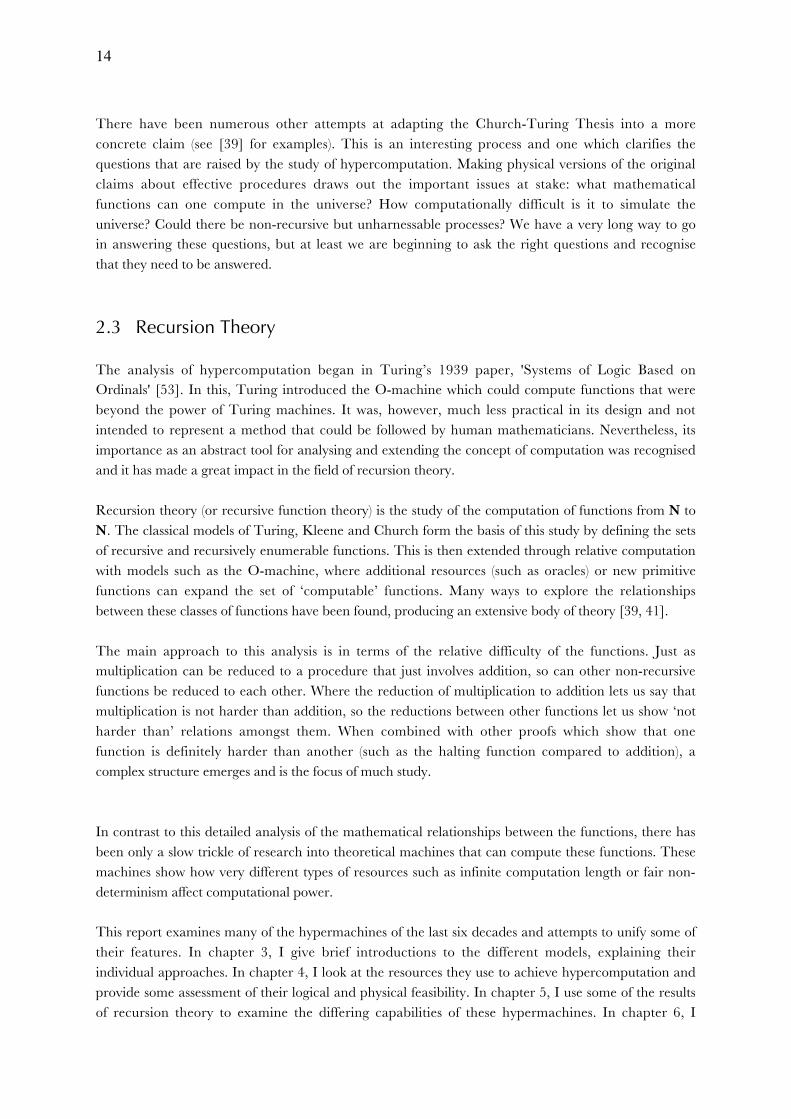
Figure 3 shows how an infinite state Turing machine can compute any function from N to {0, 1}. It isessentially an infinite lookup table which determines for all numbers given as input, what the resultshould be. By changing the dotted arcs, any such function can be specified – if f(n) = 0, then the dottedarc from state n to state f should be used (which will replace the number on the tape with therepresentation of 0), while if f(n) = 1, then the dotted arc from state n to state t should be used (which
Figure 3

20
will replace the number on the tape with the representation of 1). Either way, the transition on the arcshould be 1 / 0 / L.
As can be seen here, the tape is only used for the input and output. If one wanted to define inputs bybeginning in different states and outputs by terminating in different states, then the tape could bedispensed with altogether.
3.8 Accelerated Turing Machines
In the early 20th Century, Bertrand Russell [42], Ralph Blake [1] and Hermann Weyl [57]independently proposed the idea of a process that performs its first step in one unit of time and eachsubsequent step in half the time of the step before. Since 1 + 1/2 + 1/4 + 1/8 + … < 2, such a processcould complete an infinity of steps in two time units. The application of this temporal patterning toTuring machines has been discussed briefly by Ian Stewart [48] and in much more depth byCopeland [16] under the name of accelerated Turing machines. Since Turing’s account of his machineshas no mention of how long it takes them to perform an individual step, this acceleration not inconflict with his mathematical conception of a Turing machine.
Consider an accelerated Turing machine, A, that was programmed to simulate an arbitrary Turingmachine on arbitrary input. If the Turing machine halts on its input, A then changes the value of aspecified square on its tape (say the first square) from a 0 to a 1. If the Turing machine does not halt,then A leaves the special square as 0. Either way, after 2 time units, the first square on A’s tape holdsthe value of the halting function for this Turing machine and its input.
So far, there has been no difference between an accelerated Turing machine and a standard Turingmachine other than the speed at which it operates. In particular, A has not solved the halting problembecause Turing Machines are defined to output the value on their tape after they halt. In this case, Adoes not halt if its simulated machine does not halt. However, the situation described above suggests asimple change which will allow A to solve the halting problem – we consider the machine’s output tobe whatever is on the first square after two time units.
This model of an accelerated Turing machine only computes functions from N to {0,1}, but can beextended to functions from N to N, by designating the odd squares to be used for the special output,with each of them beginning as 0 and only being changed at most once. In this way, a natural numbercould be output in a unary representation on the special squares. This could even be extended toallowing real output, where all digits of the real would be written in binary on the special squares aftertwo time units of activity.
3.9 Infinite Time Turing Machines
This process of using an infinite computation length can be further extended. In their paper ‘InfiniteTime Turing Machines’ [29], Joel Hamkins and Andy Lewis present a model of a Turing machinethat operates for transfinite numbers of steps. We could imagine, for instance, a machine that included

21
an accelerated Turing machine (M) as a part. It could initiate M’s computation, then after two timeunits, stop M’s movements and reset M to its initial state, leaving the tape as it was at the end of thecomputation. It could then restart M with its tape head on the first tape square, running it for anothertwo time units. In such a manner, this machine would perform two infinite sequences of steps insuccession. One could even imagine a succession of infinitely many restarts, with M performing thewhole sequence twice as fast each time, leading to an infinite sequence of infinite sequences of steps.
Perhaps surprisingly, such conceptions of infinite sequences followed by further steps are well founded.The number of steps can be seen as the ordinal numbers:
0, 1, 2, 3, ... w, w+1, w+2, ... w⋅2, w⋅2+1, w⋅2+2, ... w2, w2+1, w2+2, ... ww, ...
Here the symbol w represents the first transfinite ordinal. It is also a limit ordinal, having no immediate
predecessor. After an accelerated Turing machine computes for two time units, it has performed wsteps of computation and if the tape is reused on another computation it has performed w⋅2 steps. The
infinite sequence of infinite sequences of steps is denoted by w2.
The infinite time Turing machine is a natural extension of the Turing machine to transfinite ordinaltimes. To determine the configuration of the machine at any successor ordinal time, the newconfiguration is defined from the old one according to the standard Turing machine rules. At a limitordinal time, however, the machine's configuration is defined based on all the precedingconfigurations. The machine goes into a special limit-state and each tape square takes a value asfollows:
square n at time a =
†
0, if the square has settled down to 0
1, if the square has settled down to 1
1, if the square alternates between 0 and 1 unboundedly often
Ï
Ì Ô
Ó Ô
The tape head is placed back on the first square and the machine then continues its computation fromthis limit-state as it would from any other. As usual, if there is no appropriate step to execute at somepoint, the machine halts. It can thus perform a finite amount of steps and halt, or an infinite amountof steps and halt, or keep operating through all of the ordinal times and never halt.
Such a machine could compute any recursively enumerable function in w steps, by setting the firstsquare on its tape to 0, then evaluating the function, setting the first square to 1 if f(n) = 1. If f(n) = 1,then after w steps, the first square will hold the value of 1 and if f(n) = 0, then after w steps, the firstsquare will hold the value 0. A similar method also computes any of the recursively enumerable reals.
Since infinite time Turing machines can use the entirety of their tapes during their execution, it isnatural to define them to accept infinite input (inscribed on, say, the odd squares) and produce infiniteoutput. This allows them a much greater scope in the functions they can compute, but I shall restrictmy study here to those infinite time Turing machines that take only finite input, to allow more directcomparison with the other models discussed.

22
3.10 Fair Non-Deterministic Turing Machines
Turing machines can also be generalised to behave non-deterministically [45, 49]. Where a(deterministic) Turing machine always has at most one applicable action in any circumstance, a non-deterministic Turing machine can have many. In such cases, the execution can be thought to branch,trying both possibilities in parallel. Each branch of the computation progresses exactly as it would in astandard Turing machine, except that the output is restricted to being 0 or 111. If at least one branchof the non-deterministic computation halts returning 1, then the computation is considered to return1. If there is no branch that returns 1, and at least one non-halting branch, then the computationdiverges. Otherwise (if all branches halt returning 0) then the machine returns 0.
In this manner, a non-deterministic Turing machine can be considered as using parallel processes (orlucky guesses) to quickly compute its solution. While this seems to lead to significant speedups incomputation time, it does not lead to any additional computational power. A non-deterministicTuring machine cannot compute any functions that cannot be computed by a deterministic Turingmachine. A deterministic machine can simulate a non-deterministic one by computing each of thebranches of computation in a breadth first interleaved manner. However, by restricting this non-determinism to fair computations (as done by Edith Spaan, Leen Torenvliet and Peter van Emde Boas[45]), the situation is quite different.
A computation of a non-deterministic Turing machine is said to be unfair iff it holds for an infinitesuffix of this computation that, if it is in a state s infinitely often, one of the transitions from s is neverchosen. A non-deterministic Turing machine is called fair if it produces no unfair computations12.
Spaan, Torenvliet and van Emde Boas show an interesting manner in which a fair non-deterministicTuring machine, F, could solve the halting function. F would first go to the end of its input and non-deterministically write an arbitrary natural number, n, in unary. This can be done by beginning with 0and non-deterministically choosing between accepting this number and moving on to the next stage orincrementing the number and repeating the non-deterministic choice. Once F has generated its valuefor n it can then run a bounded-time halting function algorithm, to see if the machine/input combinationhalts in n steps. If it does, F returns 1. If not, it returns 0. It is clear that if there is a time at which themachine/input combination halts, F will have a finite computation branch that returns the correctanswer (1) and F will therefore halt.
What if the given combination does not halt? In this case, the only way F will fail to halt is if it has aninfinite computation. The only place one could occur is when the arbitrary number is beinggenerated, but the only way this could not halt is by choosing to increment the number an infiniteamount of times, avoiding halting each time. This would be an unfair computation and is thus notpossible. Therefore, since all the other branches return 0, the machine will also return 0 which is thecorrect answer. In this strange way, fair non-deterministic Turing machines can compute the haltingfunction.
11 This is not essential and, like accelerated Turing machines, non-deterministic Turing machines can be thought of asreturning arbitrary natural numbers, but the presentation of them as returning only a single bit is by far the norm and isconsiderably simpler. To make this restriction, the output can be considered as whatever is on the first tape square when thecomputation halts.
12 This is just one of several types of ‘fairness’ that are discussed in the study of non-determinism.

23
Chapter 4
Resources
4.1 Assessing the Resources Used to Achieve Hypercomputation
The models discussed in the previous chapter use a wide variety of resources to increase their powerover that of the Turing machine. Many people familiar with the Turing machine paradigm and thetraditional argument that the power of Turing machines is closed under the addition of new resources(such as extra tapes and non-determinism) will find these new types of resources quite implausible.Indeed, in discussing these resources I show how some of them are logically implausible – havingsomewhat paradoxical properties – and how some are physically implausible – requiring things thatseem impossible according to current physics.
While physical implausibility is important with regards to building one of these devices, it is importantto note that our current theories about the nature of physics are far from conclusive. We must becareful not to think of arbitrary measurement and superluminal travel as impossible, but rather asimpossible relative to our best theories. Just as Newtonian physics was overturned and found to be overlyrestrictive in some areas (forbidding randomness) and overly lenient in others (allowing arbitrarily fasttravel) our current theories may also be quite removed from the truth about physics. We are thereforeunable to make claims about certain processes being physically impossible or, indeed, physicallypossible. Of course it is still very instructive to see which resources are possible or impossible withregards to our current theories.
It must also be noted that this is not a complete analysis of the implications that our current physicaltheories bear for hypercomputation. Since the resources discussed involve some of the more esotericareas of modern physics, it would be a major undertaking to give a complete account of the physicalpossibilities for hypercomputation. Instead, this section should be considered as an informal look atthe implications of physics on the hypermachines of chapter 3. I describe many physical phenomenathat are important to the realisation of a hypermachine, but do not reach any hard conclusionsregarding whether or not such machines can be built.
Even if a certain resource is physically impossible, it can still be very useful in understanding thetheory of hypercomputation. We may, for example, see that it gives equivalent power to anotherresource that is physically possible, allowing us to use the impossible resource to help us understandthe powers of the possible one. Even if no hypercomputation is physically possible at all, a study of theresources which lead to it is still important for understanding the generalised notion of an algorithm.

24
4.2 Infinite Memory
Accelerated Turing machines and infinite time Turing machines require an infinite amount ofmemory. Unlike standard Turing machines that only use a finite, yet unbounded, amount of memory,these models can require the whole tape to store their working. Therefore, building such machinesrequires a means of storing (and retrieving) an infinite bitstring. Unlike the other resources discussedin this chapter, infinite memory is not sufficient for hypercomputation, but it is necessary for somemodels.
The infinite time Turing machine explicitly requires the storage of an infinite bitstring. After a limitordinal number of time-steps, it’s state is reset to a special limit-state and its head is reset to the firstsquare, but the tape is now filled with an infinite bitstring. This bitstring is then used in furthercomputation. Infinite time Turing machines can be infinitely sensitive to the contents of their tape, sofinite approximations can not be made13.
Accelerated Turing machines seem slightly less dependent on their infinite memory, since the onlytime they use an infinite amount of memory is when they do not halt. In such cases, there is a finitetime-step at which their output is correct and will not change. If at any time after this they were to bedenied additional memory and their computation was simply halted by some external means, theresult of the computation would be unaffected. There is thus a sense in which there is no difference forthese machines between an unbounded amount of memory and an infinite amount. This is analogousto the problem of some standard Turing machines requiring an infinite amount of memory when theydo not halt. It is thus somewhat unclear as to whether an accelerated Turing machine really doesrequire the ability to store an infinite bitstring. This may be important for the physical realisation ofsuch a machine because, as discussed below, infinite memory may not be physically possible.
The storage of an infinite bitstring presents no logical problems. Indeed, it is arguably the simplest ofthe resources discussed in this chapter. We can simply use a real number or an infinite binarysequence as the state for the machine. Physical storage, on the other hand, is much more problematic.
Figure 4
An obvious method for storing an infinite bitstring is to take literally the notion of the Turingmachine’s infinite tape. We could imagine storing an infinite bitstring as an infinite series of white andblack cubes floating in space (see figure 4). The obvious disadvantage of such a system is the need forboth an infinite volume of space and an infinite amount of matter. Other methods of marking regionsof space as 0 or 1 are possible, such as with energy or even different levels of space-time curvature, butthey are all somewhat implausible with our current understanding of physics.
13 Consider an infinite time Turing machine that, after its first w steps, runs through the tape looking for a single 1 andreturning 1 if it finds one and 0 if it does not. This machine is ‘infinitely sensitive’ to the contents of its tape after the first w
steps, because any deviation from all 0’s, no matter how small, will greatly change its output. Thus some infinite time Turingmachines have zero error-tolerance.

25
Figure 5
Alternatively, we could remove the need for infinite space and resources by marking a bounded areaof space with marks of diminishing size (see figure 5). This avoids the problems discussed above, buthas the disadvantage of infinite precision being required to store the appropriate bits. According toquantum mechanics, we cannot measure any distance more accurately than the Planck length (10-35
meters), so methods like this which require arbitrarily small distances seem impossible.
Figure 6
A third approach is to use continuous values of other physical quantities (see figure 6). Because thedigits of a real can be considered as describing an infinite bitstring, being able to create and measurearbitrary real values would be sufficient for an infinite memory14. There are many quantities that wecould consider using to store the infinite bitstring, such as the velocity of a particle, the charge on acapacitor or the wavelength of a photon. Unfortunately, it looks as if all such physical variables havelimits on how accurately they can be measured [23]. If this is true, then they can only be used to storea finite amount of information.
It is therefore important to note that infinite memory is quite implausible according to our currentphysical theories. While other exotic means for storing infinite bitstrings have been considered (such asthe infinite quantum superpositions suggested in [7]), it is not at all clear that infinite memory is aphysical possibility.
4.3 Non-Recursive Information Sources
O-machines, Turing machines with initial inscriptions, coupled Turing machines, asynchronousnetworks of Turing machines, error prone Turing machines and probabilistic Turing machines allhave a classical part that is supplemented by some form of non-recursive information source. Thisconstitutes a resource that is similar but importantly different to an infinite amount of memory.
Unlike the infinite memory described previously, non-recursive information sources do not need to bechangeable. The machines mentioned in the paragraph above begin with a non-recursivespecification, but then only need a finite amount of information to describe their current state. Thus,while these machine need to be able to access an infinite amount of information, they never need tostore this much information. However, unlike the contents of an infinite memory which are slowly androutinely built up through simple steps, the initial specifications of these machines consist of non-recursive information from some external source. This is a very important distinction as it raises thequestions of where this information would come from and why we should expect it to take a certainform (such as the digits of t).
14 In contrast, the method of using marks of diminishing size only requires access to rational valued intervals.

26
The machines discussed in this section all achieve hypercomputation through conceptually differentmeans. However, when discussing them from the point of view of physical plausibility, these modelsare essentially the same. While the different conceptual resources hint at different possibilities for theirimplementation, the existence of any one of their information sources would allow us to simulate therest. For instance, if we had a non-recursive initial inscription, we could use it as an oracle for anO-machine or as a timing function for an asynchronous network of Turing machines.
How then might we gain access to a non-recursive information source to create one of the abovemachines? One way would be to find and use a real valued quantity. If we could find a rod of a non-recursive length, a particle with a non-recursive charge or even a physical constant (such as c or G )with a non-recursive value, then the process of measuring the value to greater and greater accuracywould provide another type of non-recursive information source. Since there are uncountably manyreals, but only countably many recursive reals, it seems quite plausible that many quantities may takeon non-recursive values. Unfortunately, this method suffers from the major drawback (mentioned insection 4.2) of requiring arbitrary precision measurement – this appears to be impossible according tocurrent physical theories.
A better approach may be through the observation of some non-recursive physical process. Consider,for instance, a light that flashes on and off intermittently in a non-recursive, yet deterministic, pattern.Such a light could be used to provide the non-recursive information for any of these equivalentmachines and is not in disagreement with current physical theories.
A similar process is actually found in elementary quantum mechanics. Certain particles are unstableand decay after a length of time. Such particles are said to have a half life – the length of time afterwhich the particle has a 50% chance of decaying. Thus, one could design a machine to create a seriesof such particles and observe each for one half life. If the particle decays within this time, a light couldbe flashed on, and otherwise left off. According to quantum mechanics, this pattern of flashes wouldbe completely random. Therefore, like the output of the probabilistic Turing machine discussed insection 3.6, this sequence of flashes would be non-recursive with probability one. We could then usethe bitstring produced as an oracle for an O-machine and compute non-recursive functions over thenatural numbers.
We therefore have a case of quantum mechanics suggesting very strongly that non-recursive processesexist and that the universe is not simulable by Turing machines. However, the plausibility of this non-recursive process comes at the expense of its usefulness. If the pattern of decays is really completelyrandom in the sense of probability theory (as distinct from that of algorithmic information theory),then it seems to be a perfect example of a process that is not mathematically harnessable. It mayperhaps be physically harnessable (e.g. allowing us to predict the pattern of some other process thathas been entangled with it), but it seems to be completely useless for computing definite mathematicalresults that could not be computed with a Turing machine.
Perhaps some of the other proposed non-recursive information sources may be mathematicallyharnessable. If the flashes of some light gave us the bits of t, then we could use this to compute anyrecursively enumerable function. Is it likely that the bits of t or some equivalent real would occur insome physical process? On the surface, it would seem not, but there are a couple of ways in which it

27
may be possible. For instance, it may be that there are deep links between physics and computationwhich could give rise to physical occurrences of such a computationally oriented constant.Alternatively, we may be able to engineer such an information stream – t has a very simplespecification and we may be able to constrain an otherwise unspecified stream of bits to follow it.
While a natural process giving us the bits of t does seem rather implausible, there are some equivalentprocesses that would be more believable. For example, t is known to be reducible to a function knownas the shift function15. This is a function over the natural numbers that is equal to the maximum numberof transitions that a Turing machine with n states can make before halting. A special property of thisfunction is that no function which is an upper bound for it is recursive. If we had any function thatwas an upper bound to the shift function, it would be an upper bound to the length of time a programof size n would run and would thus allow us compute the halting function. Therefore, if there is anynaturally occurring function that is an upper bound to the shift function, we can use it to compute t.
Such a method seems quite promising as it does not require the infinite accuracy of t: the physicalfunction does not need to have any deep links with theoretical computation, it just needs to grow very,very quickly.
Even if we had some hidden function that could be harnessed like this to produce t, how could we besure enough of this to use the results it gives us? We could partially check it (by seeing whether itdisagrees with some of the more simple cases that we can calculate ourselves), but we could notcompletely check that this was really t, because this would require the same amount of computationalresources as are required to generate t in the first place. How then could we have any confidence inthe accuracy of the input stream?
The only real way is if our best physical theory predicts that this process will produce the bits of t. In
this case, we would have just as much reason to believe that the input stream really was t as we havereason to believe that a physical version of a Turing machine really will operate like its mathematicalideal. Indeed, this should give just as much confidence to the accuracy of the input stream asmechanically checking it ever could, because our confidence in any checking process can not be anyhigher than our confidence in the physical theory that underlies that process. This will remain anadditional condition for all of the potential hypercomputational resources: in addition to themallowing hypercomputation, to really harness it, we must be able to scientifically justify that using theresource will give the intended results.
Unharnessable non-recursive hidden functions seem very plausible and even exist in elementaryquantum mechanics. However, harnessable non-recursive hidden functions are more difficult to comeby. There is little hope of naturally finding a sequence like t, but more hope of finding an equivalentnon-recursive function like the shift function. It is also somewhat plausible that we could engineer aspecific non-recursive sequence such as t.
15 The shift function is intimately related to the more famous (but slightly less intuitive) busy beaver function.

28
4.4 Infinite Specification
The models discussed in the previous section have a classical part (which is essentially a Turingmachine) and a separate non-classical part that can be provided through an external informationsource. In contrast, the infinite state Turing machines cannot be divided in such a way. They aretherefore naturally thought of as requiring an explicit, infinite specification.
This is highly problematic. The task of providing an arbitrary infinite specification seems far beyondanything we could hope to do. While we can understand certain infinite bitstrings (such as the binaryexpansion of π), there are only a countable amount that can be finitely expressed within any givenmathematical formalism. To gain the true power of infinite state Turing machines, we wouldtherefore require the ability to provide arbitrary infinite specifications. Such a task is clearly beyondour unaided power. Indeed, since infinite time Turing machines can be constructed to compute eachfunction from N to {0,1} using an infinite lookup table (see section 3.7), specifying an infinite timeTuring machine to compute an arbitrary function does not seem any easier than computing thefunction in the first place.
Infinite state Turing machines are therefore best regarded as theoretical models which show howallowing a Turing machine to use an infinity of states creates a degenerate kind of computer – onethat is so powerful as to trivially compute all functions from N to {0,1}. This is still an interestingresult and may lead to interesting comparisons with other infinitely specified models for computingfunctions from R to {0,1} (which would not be able to trivially compute each of these functions).However, the infinite state Turing machine is a limiting case of discrete computation and it’s methodfor achieving hypercomputation does not seem to be useful for constructing a physical hypermachine.
4.5 Infinite Computation
Performing an infinite number of steps in the computation is a very different method ofhypercomputation. The accelerated Turing machine already shows a manner in which this could bepossible: performing the steps faster and faster to get through an infinite amount in a finite time.
However, to achieve infinite computation through acceleration like this, we rapidly run into conflictwith modern physics. For the tape head to get faster and faster, it would need to get faster than thespeed of light. This is not quite a breach of the theory of special relativity as objects are allowed toexceed the speed of light so long as they are never slower than it. This is however on the very edge ofphysical plausibility.
A better approach could be to decrease the distance that the head needs to travel at each step, thusavoiding the need for exceeding the speed of light. Such an approach is adopted by Brian Davies in‘Building Infinite Machines’ [19], who also attempts to solve the problem of excessive heatproduction. This approach does have the drawback, however, of requiring infinite spatial precisionwhich has conflicts with quantum mechanics as I have discussed above.

29
Mark Hogarth [30, 31] has argued that general relativity allows infinite computation in certain exoticspace-times (known as Malament-Hogarth space-times). In such space-times, it may be possible to setup a computer and an observer in such a way that the observer witnesses the computer undertake aninfinite number of steps within a finite time. Further examination of such systems has been undertakenby Gábor Etesi and István Németi [25] who pay particular attention to the Malament-Hogarth space-time predicted to occur around a rotating, electrically charged black hole – a situation that they see asquite physically plausible. An in depth examination of Hogarth’s particular model ofhypercomputation (which differs from those presented here) can be found in Lucian Wischik’s ‘AFormalisation of Non-Finite Computation’ [58].
In their recent paper, ‘Coins, Quantum Measurements, and Turing’s Barrier’ [7], Cristian Caludeand Boris Pavlov present a model for using quantum mechanics to achieve infinite computation.Their method is quite different to the accelerated Turing machines discussed here, in that it does notperform the infinite quantity of steps in series, but rather in parallel. This gives them a distinct andinteresting way of achieving infinite computation, showing how quantum mechanical properties mayhelp hypercomputation, rather than limit it.
Leaving aside the physical difficulties with such a system, there are also some logical problems. Inparticular, there is the paradox of Thomson's lamp [51]. If we ran an accelerated Turing machinewith a program which simply replaced the first square of the tape with a 1 and then a 0 and repeatedthis procedure over and over, what would be on this square after two time units? There does not seemto be a good answer. The specification of an accelerated Turing machine made sure that one couldonly change the designated square(s) once to avoid exactly this type of problem. However, thissituation still arises on the standard parts of the tape. While we do not need to look at these squares forthe computation to work, it seems quite problematic if they may have no defined value after two timeunits.
The infinite time Turing machine avoids this by carefully defining the value of a tape square after aninfinite number of time-steps to be 0 if the symbol on the square is eventually 0 (i.e. if it becomes 0 atsome stage and then doesn't change again) and 1 if it is eventually 1 or if it alternates between 0 and 1unboundedly often. This overcomes the paradox and gives the machine a well defined behaviour, butmakes it more challenging to see how the process could be implemented.
It has also been argued (by Karl Svozil [50]) that accelerated Turing machines are paradoxical forbeing able to compute the halting function. Svozil argues that the proof that no Turing machine cancompute the halting function (because this would allow a machine with contradictory properties to bebuilt) implies that no accelerated Turing machine could compute it either. One way of avoiding thisproblem would be to say that the original proof only restricts machines from computing their ownhalting functions and we have no reason to believe that an accelerated Turing machine could do this.However, an accelerated Turing machine is exactly the same as a standard Turing machine except forits method of outputting the result. In particular, their halting behaviour is identical, thus acceleratedTuring machines can actually compute their own halting functions16.
16 Note that this is not the case for infinite time Turing machines and this counter argument therefore succeeds in defendinginfinite time Turing machines from this attack.

30
The way out of this paradox is that in the original proof, a new machine was created that solves thehalting function for a given machine and its input, halting if and only if that machine does not. Suchan accelerated Turing machine cannot be constructed. If an accelerated Turing machine is set tocompute the halting function and its input specifies a non-halting computation, this machine cannotdetermine this and then halt. Determining that this machine does not halt involves the acceleratedTuring machine looping. Thus the paradoxical machine cannot be created and the argument for thecontradictory nature of accelerated Turing machines fails17.
Unlike the accelerated Turing machine, the infinite time Turing machine can perform an infiniteamount of computation and then go on to compute more. For example, it could compute arecursively enumerable function by first computing the value of t (in an infinite number of steps) andthen using this as an oracle to compute the function (in a finite number of additional steps). Indeed,the infinite time Turing machine is in a well defined state at each ordinal time. This presents nological problem, but may well make it physically impossible.
Restricting the maximum allowable time-steps for an infinite time Turing machine gives a hierarchyof increasingly powerful machines. We can consider a standard Turing machine as an infinite timeTuring machine restricted to less than w time-steps. We can then define two types of infinite time
Turing machine for each limit ordinal l, a ‘l-time Turing machine’ and a ‘<l-time Turing machine’.Two particularly important results regarding this are Hamkins and Lewis’ result that no infinite timeTuring machine computing for an uncountable ordinal time can halt [29], and my result in chapter 5that <w2 time-steps suffice for computing all sentences of arithmetic.
We can further separate the powers of infinite time Turing machines by the number of ‘designatedsquares’ that they possess. This is just one for an accelerated Turing machine and every square for aninfinite time Turing machine, but this need not be the case. We could define Turing machines thatcompute for more than w time-steps, but can only save a finite amount of bits as they pass each limitordinal time (with the other information being lost).
We could also restrict the amount of times that the symbol on a designated square can be changed.This number is one for accelerated Turing machines and w for infinite time Turing machines, butagain this need not be the case.
These changes allow for a continuum of possible hypermachines between the power of the acceleratedTuring machines and the infinite time Turing machines. This is clearly of interest to the logical studyof infinite computation and could be of physical relevance as well, if the physical laws limitcomputation at a point between the two extreme models.
Despite potential problems with implementation, infinite computation is a very interesting theoreticalresource because it does not gain power from having additional information injected into the model,but rather allows the computation to explore every last implication of the initial information.
17Copeland [16] gives a similar argument, comparing the methods of outputting the results of each of accelerated andstandard Turing machines. He distinguishes between the ‘internal’ computation of the standard Turing machine whichallows it to use its results for further computation and the ‘external’ computation of the accelerated Turing machine whichdoes not.

31
4.6 Fair Non-Determinism
To create a fair non-deterministic Turing machine, we would either need access to some physicalprocess that directly implements fair non-determinism or a process that we could use to enforcefairness on a simulated non-deterministic system. Neither option is denied by our current physicaltheories, but there is only limited support. The most promising avenue seems to be through quantummechanics. The standard model of quantum computing (see Deutsch [22]) does not allow thecomputation of any non-recursive functions, but does use a form of non-determinism to speed up thecomputation. There may be a way to enforce fairness on such a process, but I am not aware of anymethod for doing so. The question of whether fair non-deterministic processes can exist according toour current physical theories is very much open.
On the other hand, there are reasons to be suspicious of the veryconcept of fair non-determinism. These stem from the fact thatfair non-determinism is a form of unbounded non-determinism.This means that a fair non-deterministic Turing machine, suchas F (described in section 3.10) will always halt, but can do so inan infinite number of different ways (generating any n Œ N inthe process). Gordon Plotkin [40] points out a tension betweenthis and König’s lemma (which states that if all branches of afinitely branching tree are finite, then so is the tree itself). Plotkinargues that therefore the computation tree of F must have aninfinite branch and hence the possibility of non-termination (seefigure 7 for the computation tree involved in F’s generation of n).However, as pointed out by William Clinger [12], it is possiblethat the computation tree does indeed contain an infinite branchwhich has each of its nodes present in one of the halting computations, but there does not need to beany single computation that proceeds all the way down the infinite branch. This counters Plotkin’sargument, but shows that fair non-determinism has some very unintuitive consequences.
Another example of the unintuitive nature of fair non-determinism can be seen in the behaviour of F.Recall that F computes the halting function by generating an arbitrarily large integer, n, and testing tosee if the given machine halts on its input within n time-steps. If the simulated machine halts, then wewould imagine that the time taken by F is related to the smallest value of n that was required. What ifthe simulated machine does not halt? In this case we know that F will return 0, but it is entirelyunclear as to how this will happen. This problem becomes particularly noticeable when we considerthe length of time F will take to return its result. If we consider the non-determinism as computingeach branch in parallel, then we would assume that the machine would halt when all the brancheshave halted, however, even though each branch halts, there is no time at which they have all halted.Although this machine has no infinite branch, its infinite sequence of increasingly long finite branchesseem to keep it from halting just as effectively.
The status of fair non-determinism is therefore somewhat unclear. There do not seem to be any strongreasons to believe that it is physically impossible, but its logical consequences are quite unintuitive andneed to be better understood before we can be sure that it is free of internal contradiction.
Figure 7

32
Chapter 5
Capabilities
5.1 The Arithmetical Hierarchy
Following recursion theory, we can develop a means of assessing the relative powers of differenthypermachines by examining the sentences of arithmetic. These are well formed formulae composedof natural numbers, variables ranging over natural numbers, +, ⋅, ÿ , Ÿ, ⁄, ", $, =. These formulaeinclude many elementary statements such as:
3 does not divide 8: ÿ$x (8 = 3⋅x)
Addition is commutative: "x "y (x + y = y + x)
It is also possible to express more complex statements about the natural numbers whose truth is muchless clear. Indeed, it is this language for which Gödel proved his incompleteness theorem – noconsistent formal system can prove all the true formulae of arithmetic. In his proof [27], Gödelshowed how predicates could be constructed in this language through leaving free variables in theformula. For example, we can have:
x | y: $z (x = y⋅z)
Prime(x): ÿ(x = 1) Ÿ ÿ$z ( ÿ(z = 1) Ÿ ÿ(z = x) Ÿ x|z )
It is this form of ‘programming’ in the language of arithmetic that Gödel used to construct thepredicate ‘is provable in Principia Mathematica’. From this, he created his famous statement thatclaims it is unprovable within Principia Mathematica. Gödel’s generalisation of this argument to findunprovable statements for all formal systems shows that this language of first order arithmetic is veryexpressive.
The full power of its expressiveness was explored much more fully by Kleene [34] who stratified thepredicates expressible in first order arithmetic into what is called the arithmetical hierarchy. This consistsof the classes Sn, Pn, Dn, where n ΠN. These are defined as follows18:
18 Note that I only look at formulae with one free variable (and thus predicates of one variable). This can be done withoutloss of generality because of the existence of recursive mappings from Nm to N.

33
S1: {x : $y ( R(x, y) )} where R is a recursive relationP1: {x : "y ( R(x, y) )} where R is a recursive relation
Sn: {x : $yn ( P(x, y1,..., yn) )} where P is a Pn-1 relationPn: {x : "yn ( S(x, y1,..., yn) )} where S is a Sn-1 relation
From these, we define:Dn: Sn « Pn
Figure 8 shows the large-scale structure of the arithmetical hierarchy, withthe arrows representing strict set inclusion. Sw represents the union of Sn for
all n and similarly for Pw and Dw.
Of particular note, D1 is the set of recursive relations, S1 is the set ofrecursively enumerable relations and P 1 is the set of co-recursivelyenumerable relations. We can see, for instance that the relation defined bythe halting function is in S1 by considering that the relation HaltsBy(x, t)that is true if and only if the Turing machine and input encoded by x haltswithin t time-steps. HaltsBy is clearly recursive and thus $t ( HaltsBy(x, t) ) –which represents the halting relation – is in S1. Similarly, we can show thatthe relation defined by the looping function can be represented as"t ( ÿHaltsBy(x, t) ) and thus is in P1.
The usefulness of the arithmetical hierarchy is expanded by the following theorems:
The representation theorem:For any relation R, R is in the arithmetical hierarchy iff R is definable in elementary arithmetic
The strong hierarchy theorem:R Œ Dn+1 iff R is recursive in ∅(n) (i.e. the nth jump of the empty set as discussed in section 3.1)R Œ Sn+1 iff R is recursively enumerable in ∅(n)
R Œ Pn+1 iff R is co-recursively enumerable in ∅(n)
5.2 Comparative Powers
The arithmetical hierarchy therefore gives us a generalisation of the concepts of recursiveness andrecursive enumerability which allow us to measure and compare the power of the hypermachines thathave been explored. This power is measured in terms of the predicates over N that can be computedby each hypermachines. This generalises to functions from N to {0,1}, sets over N, or computablereals.
Figure 8

34
D1: Turing machinesO-machines with ∅ oracle (or any recursive oracle)
Turing machines with ∅ initial inscription (or any recursive inscription)asynchronous networks of Turing machines with recursive timing functionserror prone Turing machines with recursive error functionscoupled Turing machines with recursive coupled functionsprobabilistic Turing machines with recursive random choices
S1: fair non-deterministic Turing machines19
accelerated Turing machines20
D2: O-machines with ∅' oracleTuring machines initially inscribed with ∅'infinite time Turing machines (in w time-steps)21
Dn+1: O-machines with ∅(n) oracleTuring machines initially inscribed with ∅(n)
infinite time Turing machines (in w⋅n time-steps)
Dw: O-machines with ∅(w) oracleTuring machines initially inscribed with ∅(w)
infinite time Turing machines (in <w2 time-steps)
There is also a large collection of machines that can compute all predicates over the natural numbers.This involves much more power than can be expressed in the arithmetical hierarchy (there areuncountably many predicates over N, but only a countable subset are expressible in the arithmeticalhierarchy).
every predicate over N:O-machine (with arbitrary oracle)Turing machine (with arbitrary initial inscription)coupled Turing machines (with arbitrary coupled function)error prone Turing machines (with arbitrary error function)asynchronous networks of Turing machines (with arbitrary timing functions)probabilistic Turing machines (with arbitrary random events)
infinite state Turing machine
19 For a proof of this, see [45].
20 For a proof of this, see the appendix.
21 The results for the power of infinite time Turing machines with limited time-steps are lower bounds only. The upperbounds are not known, but I would be quite surprised if they are different. For the proofs, see the appendix.

35
Finally, while infinite time Turing machines can be shown to compute all predicates expressible in firstorder arithmetic in <w2 time-steps, the set of predicates that they can decide in arbitrary time exceedsthe arithmetical hierarchy. The exact power is unknown, but is clearly much less than all predicatesover N (since there are only countably many infinite time Turing machines).
Some of these results have particularly interesting consequences. For instance, consider the modelsthat can compute exactly the S1 predicates. These models can compute the halting function, returning1 if the program halts on its input and 0 otherwise, but cannot compute the looping function whichwould only require negating this result. This is quite an interesting result, because while acceleratedTuring machines and fair non-deterministic Turing machines can compute both the halting functionand the negation function ( f(x) = 1 - x ), they cannot compute the composition of these functions. Thefunctions computable by these models are thus not closed under composition, which is most unusualamongst serious models of computation. Since we would expect the functions computable by physicalmachines to closed under composition (the output of one machine can be used as input of another)and we know that negation is computable by physical machines, it seems highly implausible that S1 isthe limit of physical computation available in our universe.
The absence of closure under function composition also makes these models somewhat strange astheoretical devices. Indeed, it is probably best to imagine such devices as part of a larger machine. AsCopeland [16] shows, we could embed one of these devices inside a Turing machine as an oracle.Since they can function as oracles for ∅', the resulting O-machine could compute the entirety of D2.
It is also of special interest that some of these hypermachines can compute Dw. This means that theycan compute all the predicates that can be expressed as sentences in first order arithmetic. From theRepresentation Theorem, we can see that this includes all formulae of arithmetic that have freevariables. What about those that do not have free variables? Consider an arbitrary formula ofarithmetic that has no free variables. This sentence must include an = symbol because it is the onlyway of constructing an atomic formula in this language. We can construct a new formula by addingthe term ‘+ x’ (where x is a new variable) to one side of the = sign. This gives us a new formula inarithmetic which expresses a predicate and is thus computable by this group of hypermachines. Inparticular, these hypermachines can compute the answer when x is equal to 0. In such a case, thisformula is true if and only if the original formula is true. Thus, hypermachines that can compute Dw
can compute the truth of all sentences of arithmetic.
This is not a violation of Gödel’s Incompleteness Theorem because his theorem only applies to formalsystems (which are defined to have the same computational power as Turing machines). Gödel’smethods cannot construct a true but unprovable sentence for these hypermachines because theirworkings cannot be captured in first order arithmetic. This result obviously has considerableimplications for the common (mis)interpretation of Gödel’s Incompleteness Theorem as stating thatno conceivable machine can prove exactly the true sentences of arithmetic.
It is also important to consider the implications of those models that can compute all predicates overthe natural numbers. Doing so requires an uncountable infinity of machines – at least one perpredicate. Thus, the machines require infinite specifications (in most cases, this corresponds to

36
specifying the non-classical part as well as the classical part). It is not at all clear how we should do so.While some infinite specifications are finitely definable in, say, first order arithmetic, each languagewith a finite alphabet has only a countable amount of finite strings. This is not enough to specify allthe machines, so any attempt to finitely specify these machines through the use of a mathematicalformalism must either use an infinite alphabet or infinitely many mathematical languages. Neithercase looks any simpler than the original infinite specifications. It thus seems that while the universemay well have processes that behave according to these models, we will never be able to harness themto compute arbitrary functions.
Machines that can compute all predicates over N also seem to be of little theoretical interest. All ofthose examined here can compute a given predicate over N using a simple infinite lookup table (seethe study of infinite state Turing machines in section 3.7 for a good example of this). They thereforedo not need any algorithmic sophistication to compute these predicates. This is a similar situation toTuring machines computing predicates over a finite set – the machines are so powerful compared tothe problem that only a degenerate kind of computation occurs.

37
Chapter 6
Implications
6.1 To Mathematics
One of the first uses of the Turing machine model was to show that the Entscheidungsproblem (thedecision problem for the predicate calculus) is undecidable. By the Church-Turing Thesis, allfunctions computable by unaided mathematicians working without insight are computable by aTuring machine and since there is no Turing machine to solve the decision problem for predicatecalculus, it was concluded that no unaided mathematician could solve it without insight.
The concept of hypercomputation sheds new light upon this and similar results. It prompts us to askwhether the Entscheidungsproblem could be solved by a mathematician that was aided by some kindof machine. The answer to this is not within the domain of mathematics. Instead it depends on thenature of physical reality. If it is possible to harness physical processes to build a hypermachine, then amathematician may well be able to use this to decide whether arbitrary formulae of predicate calculusare tautologies.
Thus the claims that such problems are ‘undecidable’ or ‘unsolvable’ are misleading. As far as weknow, in 100 years time these problems might be routinely solved using hypermachines.Mathematicians may type arbitrary diophantine equations into their computers and have themsolved. Programmers may have the termination properties of their programs checked by some specialsoftware. We cannot rule out such possibilities with mathematical reasoning alone. Indeed, even thetruth or otherwise of the Church-Turing Thesis has no bearing on these possibilities. The solvability ofsuch problems is a matter for physics and not mathematics22.
To show that a problem is physically undecidable should be a two part process. First, wemathematically determine how difficult the problem is using the techniques of recursion theory. Thenwe must ascertain whether or not it is physically possible to solve problems of that level of difficulty.Traditional arguments for undecidability have only focussed on the first of these steps, assuming that
22 A similar view is held by Deutsch, Ekert and Luppachini [24] who state that ‘though the truths of logic and puremathematics are objective and independent of any contingent facts or laws of nature, our knowledge of these truths dependsentirely on our knowledge of the laws of physics’. See also Deutsch [23] for a further discussion of his view on therelationship of physics to mathematics.

38
no non-recursive function is physically computable. This often unstated assumption is not only a verystrong claim about the nature of our universe, but also lacking in physical evidence. It is not amathematical claim and it is not appropriate to use it in a mathematical proof for anything more thanspeculation about the physical implications.
This distinction that I am drawing between the mathematical and physical sides to an undecidabilityresult generalises to Chaitin’s results about randomness in mathematics.
Chaitin proved that W is ‘random’ and that its non-recursive information is so much more dense than
t that no formal system of size n bits can determine more than n bits of W. He has also shown thatanalogous results occur in arithmetic, leading to systems of equations whose solutions do not have anyrecursive pattern. These results are nothing short of spectacular, but they are only results about thecomplexity of W relative to Turing machines and formal systems that are equally powerful. While it issometimes claimed [4, 10] that W is completely patternless, this is not true. If it was, it would not be so
easily describable. Indeed W is recursively enumerable and thus computable by every hypermachinepresented in this paper. If a single one of these hypermachines can be built, we may well see peoplecomputing the digits of W as they now compute the digits of π.
Chaitin’s results about W show not that some mathematical objects are patternless, but that they seempatternless relative to a certain amount of computational power23. The results do not show that somefacts (such as the value of a particular bit of W ) are true for no reason, but that a certain level ofcomputational power is insufficient to show why these facts are true. If hypercomputation is found tobe physically impossible, then we could expand these results, with our universe itself being insufficient tofind pattern in W or reasons for its digits being what they are. In any event though, it is not an absenceof pattern, but rather a complexity of pattern, or an inaccessibility of pattern.
Gödel’s results are similarly affected. While he successfully showed that no formal system can prove alltruths of arithmetic, the implications that are commonly drawn from this are flawed. Even in theforeword of Davis’ The Undecidable [20] we are told Gödel proved that ‘systems of logic, no matter howpowerful, could never admit proofs of all true assertions of arithmetic’. While this particular claim isperhaps more careless than misguided, it is indicative of the general presentation of Gödel’s results.What he really showed was that no formal system of equivalent power to the Turing machine couldenumerate all of the truths of arithmetic.
Many other systems of logic with non-recursive sets of axioms or rules of inference are possible. Onecould, for example, program an infinite time Turing machine or an O-machine with ∅(w) oracle toenumerate all the truths of arithmetic. It certainly requires a lot of computational power to prove allthese truths with no falsehoods, but there are systems of logic which achieve this and it may even bephysically possible to implement them. What we can mathematically prove depends on physics. Inuniverses with different physics, different levels of computation would be possible and thus differentsets of theorems would be provable from a given set of axioms24.
23 See section 6.3 for a more detailed development of this idea.
24 See Deutsch [23] for a similar claim about the dependency of mathematical reasoning on physics.

39
And so each of these famous negative results does not go so far as is commonly argued. Thelimitations present in the results of Gödel, Turing and Chaitin are all relative to Turing machines. Asfar as we know, it may soon be routine to decide the truth of arbitrary statements of arithmetic, solvethe halting problem and compute the digits of W. To find out, we need to complete the second part ofthe method mentioned above. The difficulty of these tasks has been determined – now we need to findout whether the universe has enough resources to compute them.
Even if it does, the ideas of Gödel, Turing and Chaitin are still very relevant. As well as showing thelimits of Turing machines, they present a general method for finding problems that are unsolvable fora given type of machine. Presumably, we will find similar cases of incompleteness, undecidability andrandomness relative to our most powerful implementable machines, whatever they happen to be. Myargument is not with the limitation of our mathematical knowledge, but rather that we so far have nospecific examples which we can say are incomplete, uncomputable or random relative to our physicallaws.
6.2 To Physics
Computability is a very important physical issue. As argued above, the fundamental questionregarding how much we can compute is a question of physics, and not mathematics as has beentraditionally believed. We are now quite familiar with other physical limits such as the speed of light,the second law of thermodynamics or the conservation of energy. As we become more aware of theimportance of computation at both fundamental and everyday levels, our lack of a physical principleexplaining the limits of computation becomes more glaring.
Feynman [26] was the first to address such a gap in terms of the limits of computational efficiency,introducing the idea of quantum computing in order to close the apparent gap between what can besimulated efficiently and what can happen (efficiently) in quantum mechanics. His idea of harnessingthese computationally complex results that nature was producing so quickly in quantum systemsslowly built up the field of quantum computation which seriously addresses the issues of the universe’slimits for the efficiency of computation.
We are perhaps seeing the beginning of a similar movement for exploring the physical limits ofcomputational power. A few physicists have recently suggested possible ways that quantum mechanicsand relativity may allow not only complexity gains, but computational gains. Hogarth [30, 31] hasargued that general relativity may allow an infinite number of steps to be performed in a finite time.Calude and Pavlov [7] have shown how quantum mechanics may allow an infinite amount of steps tobe performed in parallel, allowing a stochastic solution to non-recursive functions. Kieu [32]demonstrates a similar result.
There has also been some interest by physicists in exploring the fundamental connections betweencomputation and physics. Deutsch [22, 23, 24] explores such connections, speculating on the limits ofcomputation and addressing the fundamental question of how difficult it is to simulate the universe.He proposes the ‘Church-Turing Principle’: that the universe is capable of containing a universalmachine that can simulate arbitrary systems of the universe.

40
In chapter 2, I presented my own physical theses about the physical limitations of the universe,suggesting ways in which the universe may not be self-simulable due to an absence of harnessablehypercomputation. I also made a distinction between mathematical and physical harnessability,showing how it may be possible for the universe to be unsimulable through a mathematicalrepresentation, but still simulable. A universe that is classically simulable, but for the existence of anumber of rods of the same non-recursive length is such an example. We may be able to use one ofthese rods to simulate the others even if we cannot produce a finite mathematical description of itslength. Such possibilities present new challenges for the foundations of physics and the philosophy ofscience.
6.3 To Computer Science
Hypercomputation clearly has considerable implications for computer science, yet it has receivedalmost no attention there. Part of the reason for this is that few people realise that it is logicallypossible to exceed the power of the Turing machine. It is often believed that the Church-TuringThesis rules out the possibility of hypercomputation. Another common misconception is that the proofof the uncomputability of the halting function by Turing machines makes it paradoxical for anymachine to compute it. Finally, people dismiss the possibility of hypercomputation as completelyunrealistic or in violation of some physical laws.
The first two of these reasons for ignoring the possibility of hypercomputation are simply false. Thethird would have some force if it was used with an understanding of the many different resources thatcould be used to achieve hypercomputation, but there has been no detailed analysis of whether theseresources are physically realisable. It is thus very unfortunate that the reasons above have caused somany people to ignore the fascinating possibilities that hypercomputation offers.
One of the main reasons that people still hold these misconceptions is that the basic issues ofhypercomputation – particularly those three just mentioned – are often not well understood andconsequently the possibility of hypercomputation is not presented in textbooks or lectures. While thereare exceptions to this (most notably brief presentations of O-machines), students still tend to finishtheir computer science education with a firm belief that the Turing machine has limits on itscomputation, but that it is as powerful (in terms of computability) as any other possible machine.
There are very important issues regarding computability at stake here. What forms can an algorithmtake? What is computable in our universe? These are questions that one would expect to attract manyresearchers. They are unanswered (and relatively unexplored) questions that are of great importanceto computer science.
One example of the gains that can be made by applying the lessons of hypercomputation to classicalfields is in algorithmic information theory. Hypercomputation provides a very natural relativisation ofalgorithmic information theory. Previously, we looked at algorithmic information theory in thecontext of a person, Alice, sending compressed messages to a friend, Betty, who uses a Turingmachine to decode them. Of particular interest was the case of sending infinite messages. For some

41
messages (such as the digits of π) there is a finite program that can be sent instead. For others (such asthe digits of t) there is no finite program that can be sent which generates this sequence. Thus if Alicesomehow has access to t, she needs to send an infinite number of bits to Betty to share this
information with her. It can thus be said that t contains an infinite amount of algorithmicinformation.
As was discussed in chapter 1, for Betty to receive n bits of t, Alice only needs to send log(n) bits ofinformation because t’s information is spread very thinly. For W on the other hand, Alice needs tosend n bits for Betty to determine n bits, thus W is said to be random.
In a relativised algorithmic information theory, we can provide Betty with different types of computer. Forexample, consider a faulty Turing machine that can only move its tape head to the right. It can beshown that such a machine can compute all the rationals, but no irrational numbers. Therefore, ifAlice and Betty were restricted to such machines and Alice wanted to send the number π to Betty, shewould be forced to send an infinite bitstring. With this model of computation, π has an infiniteamount of algorithmic information.
We can also look at what happens when Betty has access to a hypermachine. If Betty has access to,say, an O-machine with the halting function oracle, then Alice can send her a finite program forcomputing t or W. Relative to an O-machine with the halting function oracle, t and W both havefinite algorithmic information. However, the bits that describe this machine’s halting function (or thetruths of arithmetic) would still require an infinite message.
With a relativised algorithmic information theory, we would say that t contains an infinite amount ofinformation relative to a Turing machine, that W is random relative to a Turing machine and that πcontains an infinite amount of information relative to a ‘right-moving Turing machine’.
This appears to be a deep and natural generalisation from the standard theory and is not limited byany reliance on the actual computational power of our universe. Instead, it provides a concept ofinformation that is relative to the level of power available and thus relative to our particular laws ofphysics. By exploring the ideas involved in hypercomputation, we should be able to generalise andextend the classical results of other areas of computer science in a similar manner. A study ofcomplexity theory over these machines, for instance, would no doubt be very interesting andilluminating.
Finally, if we can actually build any of these hypermachines, there will obviously be large implicationsfor computer science. Hypercomputation would presumably become mainstream computer science aspeople move to take advantage of these new powers. It is worth noting that the uptake ofhypercomputation could still be limited by such things as impractical construction, price, or evenspeed of computation – it may be that the only buildable hypermachines are exponentially slowerthan Turing machines. In any event, there is no doubt that if we discover that hypercomputation isphysically possible and harnessable, its implications to computer science will be immense.

42
6.4 To Philosophy
The possibility of hypercomputation also bears important implications in several branches ofphilosophy. One of these is the philosophy of mind. The computational theory of the mind looks atthe possibility that the computations performed in the brain give rise to the mind. It is often claimedthat if the mind is indeed computational in nature, then we could simulate the brain (and mind) on aTuring machine. This argument often appeals to the Church-Turing Thesis to show that allcomputation can be simulated on a Turing machine. This mistaken belief in the power of the Church-Turing Thesis pervades the literature and is discussed in great depth by Copeland [13]. Copeland alsoshows how the claims made in the computational theory of mind can be generalised to allow for thepossibility of hypercomputational processes in our brains giving rise to our minds [15].
Hypercomputation also has significant implications in epistemology. In classical computation, there isa fixed limit to the conclusions that can be validly generated from a set of premises, buthypercomputation generalises this with the amount of valid inferences growing with the level ofcomputational resources available. This not only relativises provability and inference, but makes theactual amount of inference that is possible in the real world dependent upon the true nature of physicsand not a priori as it is generally believed.
In addition, epistemology involves assessing the complexity of different ideas. Simplicity is a crucialnotion when deciding which of two theories to prefer and thus the changes to algorithmic informationtheory brought about by hypercomputation become relevant. To measure the complexity of a theory,we must do so relative to a given level of computational power and thus an understanding ofhypercomputation seems necessary here.
It is not clear how large the impact of hypercomputation in these areas will be, but it should not beoverlooked. Several areas of philosophy involve computational concepts and the widespread lack ofknowledge about hypercomputation will no doubt have caused important possibilities to beoverlooked. Hypercomputation is very relevant to philosophy and must be accepted as a logicalpossibility that needs careful consideration and investigation.

43
Chapter 7
Conclusions and Further Work
7.1 Conclusions
Models of computation that compute more than the Turing machine are conceptually unproblematicand may even be buildable. This has many important implications. The most direct of these is thatmathematical proofs that certain functions are ‘uncomputable’ must be more clearly understood asshorthand for ‘uncomputable by a Turing machine’ and not as a limitation on mathematics. As I haveargued in chapters 5 and 6, the proofs of incompleteness and randomness in arithmetic must also beseen as merely relative to Turing machines. By opening the possibility of physical machines thatcompute the halting function, W and all the truths of arithmetic, hypercomputation shows us that thegreat negative results of 20th Century mathematics are not so negative as it was first believed.
In doing so, hypercomputation follows its analogue in complexity theory – quantum computation – inelucidating the connections between mathematics, physics and computer science. As quantumcomputation showed that mathematics alone cannot provide the limits of physically practicalcomputation, so hypercomputation shows that mathematics alone cannot provide the outer limit forphysically possible computation.
In chapter 2, I looked at three different ways in which physical computation could be limited. It maywell be that there are physical processes that, while not simulable by a Turing machine, are notharnessable for the computation of any particular non-recursive functions. Furthermore, it may bethat there exist non-recursive physical processes that cannot be simulated with the resources availablewithin the universe. The logical independence of the computational limits on physical processes,physically harnessable processes and mathematically harnessable processes allows many different waysin which our universe could be hypercomputational – each with its own implications for physics andthe philosophy of science.
With the increasing understanding of the misconceptions surrounding the Church-Turing Thesis,prematurely closed possibilities – such as a hypercomputational theory of mind – can be explored.Through non-classical models of computation, such as infinite time Turing machines, we can alsoattempt to gain a deeper understanding into the nature of algorithms. Regardless of the actualcomputational limits of our universe, I have no doubt that the study of hypercomputation will lead tomany important theoretical results across computer science, philosophy, mathematics and physics.

44
7.2 Further Work
The ideas explored in this report are only the very beginnings of a comprehensive theory ofhypercomputation and there are thus many avenues for further work.
Theses B, C and D , in chapter 2 provide interesting insights into different computational limits inphysics. However, they rely on the terms ‘simulable’, ‘mathematically harnessable’ and ‘physicallyharnessable’. While I have tried to give useful definitions of these terms, more work is required tocreate precise concepts with which to assess the availability and usefulness of hypercomputation in ouruniverse. This is quite related to the problem of defining what it means for a physical process tocompute a given function and – while there are some difficulties with this – the techniques used byCopeland [12] and Deutsch [22, 23] look particularly promising.
While the theses I have provided present an interesting stratification of the computational powers ofdifferent possible universes, they could be extended to provide a more fine-grained classification. Inparticular, there would be considerable benefit in extending them to assess the universe’s simulabilityby arbitrary models of computation instead of just Turing machines. It would also be beneficial toexplore the relationship between my theses and Deutsch’s Church-Turing Principle.
In this report, I have not had the space to present every hypermachine that has been explored. Inparticular, I have not been able to look at non-uniform circuit families, type-2 machines [56], HavaSiegelmann’s processor networks [43] or Lenore Blum, Mike Shub and Steve Smale’s machines forcomputation on arbitrary rings (BSS machines) [2]. The presentation of these models and the linkingof them into the framework of this paper would obviously be of great use.
In chapter 4, I looked briefly at a way of exploring models between the power of an acceleratedTuring machine and an infinite time Turing machine. I have given only a few proofs and results aboutsuch machines in this paper and a formal presentation of such machines and their capabilities wouldbe most interesting.
It would also be of considerable interest to examine the more ‘realistic’ resources of interaction andinfinite run-time as discussed by Jan van Leeuwen and Jirí Wiedermann [55]. They present goodarguments for requiring a new model for the study of such machines due to their increased power overTuring machines. Looking at this in the context of hypercomputation may provide some useful resultsfor the study of these systems.
In studying the capabilities of the hypermachines in this report, my use of the arithmetical hierarchyrestricted my analysis to functions from N to {0,1} (or equivalently, reals or sets of naturals). It wouldbe very nice to be able to extend this analysis to functions from N to N, providing a complete accountof the capabilities of these machines. It would also be useful to discuss the capabilities of variousmachines that compute over R, including infinite time Turing machines, type-2 machines and BSSmachines.

45
I have also only been able to give a brief introduction to the relativisation of algorithmic informationtheory to arbitrary computers. This is a very promising area which is practically unexplored. An in-depth look at the generalised notions of incompressibility and randomness would provide considerableinterest.
While I have shown that there are generalised algorithms for enumerating the truths of arithmetic,computing the halting function and computing W, there is a strong sense in which we remain underthe shadow of incompleteness, uncomputability and randomness. It seems as though the methods usedby Gödel, Turing and Chaitin to show these limitations of mathematics can be extended to modelsbeyond the Turing machine. Indeed it seems quite likely that while these famous arguments do notestablish any absolute limits for mathematics, they can be used to construct similar limitations for anyparticular model of computation. Whether or not this can be achieved, and the exact form that suchgeneralised arguments would take is of considerable interest and is certainly a key area for furtherresearch.

46
References
[1] Ralph M. Blake. The Paradox of Temporal Process. Journal of Philosophy, 23:645-654, 1926.
[2] Lenore Blum, Mike Shub and Steve Smale. On a Theory of Computation and Complexity over theReal Numbers: NP-Completeness, Recursive Functions and Universal Machines. Bulletin of the AmericanMathematical Society, 21:1-46, 1989.
[3] Olivier Bournez and Michel Cosnard. On the computational power and super-Turing capabilities ofdynamical systems. Technical Report No. 95-30, Laboratoire de l’Informatique du Parallelism, EcoleNormale Superieure de Lyon, 1995.
[4] Cristian S. Calude and Arto Salomaa. Algorithmically Coding the Universe. Pages 472-492 in G.Rozenburg and A. Salomaa, editors. Developments in Language Theory. World Scientific, Singapore, 1994.
[5] Cristian S. Calude, J. Casti and M. J. Dineen, editors. Unconventional Models of Computation. Springer-Verlag, Singapore, 1998.
[6] Cristian S. Calude and Michael J. Dinneen. Breaking the Turing Barrier. Technical ReportCDMTCS-084, Department of Computer Science, University of Auckland, New Zealand, 1998.
[7] Cristian S. Calude and Boris Pavlov. Coins, Quantum Measurements and Turing’s Barrier. Availableonline at the Los Alamos Archive (http://xxx.lanl.gov/), arXiv:quant-ph/0112087, 2002.
[8] Gregory J. Chaitin. On the Length of Programs for Computing Finite Binary Sequences. Journal of theAssociation of Computing Machinery, 13:547-569, 1966.
[9] Gregory J. Chaitin. Algorithmic Information Theory. Cambridge University Press, Cambridge, 1987.
[10] Gregory J. Chaitin. An Invitation to Algorithmic Information Theory. Pages 1-23 in DMTCS’96Proceedings, Springer-Verlag, Singapore, 1997.
[11] Alonzo Church, An unsolvable problem of elementary number theory, American Journal of Mathematics,58:345-363, 1936. Also in Davis [20]
[12] William D. Clinger. Nondeterministic call by need is neither lazy nor by name. Pages 226-234 inSymposium on LISP and Functional Programming. Pittsburgh, Penn., 1982.
[12] B. Jack Copeland. What is Computation? Synthese, 108:335-359, 1996.
[13] B. Jack Copeland. The Broad Conception of Computation. American Behavioural Scientist, 40:690-716,1997.
[14] B. Jack Copeland. Super Turing-Machines. Complexity, 4:30-32, 1998.
[15] B. Jack Copeland. Turing's O-Machines, Penrose, Searle, and the Brain. Analysis, 58:128-138, 1998.
[16] B. Jack Copeland. Even Turing Machines Can Compute Uncomputable Functions, pages 150-164. InCalude [5], 1998.

47
[17] B. Jack Copeland and Richard Sylvan. Beyond the Universal Turing Machine. Australasian Journal ofPhilosophy, 77:46-66, 1999.
[18] Felipe Cucker and Dima Grigoriev. On the power of real Turing machines over binary inputs. SIAMJournal on Computing, 26(1):243-254, 1997.
[19] E. Brian Davies. Building Infinite Machines, British Journal for Philosophy of Science, 52:671-682, 2001.
[20] Martin Davis, editor. The Undecidable, Raven Press, 1965.
[21] John W. Dawson. Logical dilemmas: the life and work of Kurt Gödel. Wellesley, Mass., 1997.
[22] David Deutsch, Quantum Theory, the Church-Turing Principle and the Universal QuantumComputer. Proceedings of the Royal Society, Series A 400:97-117, 1985.
[23] David Deutsch, The Fabric of Reality. Penguin, London, 1997.
[24] David Deutsch, Artur Ekert and Rossella Luppachini. Machines, Logic and Quantum Physics. Bulletinof Symbolic Logic, 3:265-283, 1999
[25] Gábor Etesi and István Németi. Non-Turing computations via Malament-Hogarth space-times.Available online at the Los Alamos Archive (http://xxx.lanl.gov/), arXiv:gr-qc/0104023, 2002.
[26] Richard P. Feynman. Simulating physics with computers. International Journal of Theoretical Physics,21:467-488, 1982.
[27] Kurt Gödel. On Formally Undecidable Propositions of Principia Mathematica and Related Systems I,pages 5-38 in Davis [20], 1931.
[28] Kurt Gödel. On Undecidable Propositions of Formal Mathematical Systems, pages 41-74 in Davis[20], 1936.
[29] Joel D. Hamkins and Andy Lewis. Infinite Time Turing Machines. Journal of Symbolic Logic, 65:567-604,1998.
[30] Mark L. Hogarth, Does General Relativity Allow an Observer to View an Eternity in a Finite Time?Foundations of Physics Letters, 5:173-181, 1992.
[31] Mark L. Hogarth, Non-Turing Computers and Non-Turing Computability, PSA, 1:126-138, 1994.
[32] Tien Kieu. Computing the noncomputable. Available online at the Los Alamos Archive(http://xxx.lanl.gov/), arXiv:quant-ph/0203034, 2002.
[33] Stephen C. Kleene. General recursive functions of nautral numbers. Mathematishe Annelen, 112:727-742,1936. Also in Davis [20].
[34] Stephen C. Kleene. Recursive predicates and quantifiers, Transactions of the American Mathematical Society,53:41-73, 1943.
[35] Andrei N. Kolmogorov. Three Approaches to the Quantitative Definition of Information. ProblemsInformation Transmission 1:1-7, 1965.
[36] Georg Kreisel. Mathematical logic. Pages 95-195 in Saaty, editor, Lectures on modern mathematics, vol. 3,Wiley and Sons, New York, 1965.
[37] Karel De Leeuw, Edward F. Moore, Claude E. Shannon, N. Shapiro. Computability by probabilisticmachines. Pages 183-212 in C. E. Shannon and J. McCarthy, editors, Automata Studies, PrincetonUniversity Press, Princeton, N.J., 1956.
[38] Thomas J. Naughton and Damien Woods. On the computational power of a continuous-space opticalmodel of computation. Technical Report NUIM-CS-TR-2001-01, Department of Computer Science,National University of Ireland, Maynooth, 2001.
[39] Piergiorgio Odifreddi. Classical Recursion Theory. Elsevier, Amsterdam, 1989.

48
[40] Gordon D. Plotkin. A powerdomain construction, SIAM Journal on Computing, 5:452-487, 1976.
[41] Hartley Rogers Jr. Theory of Recursive Functions and Effective Computability. McGraw-Hill, 1967.
[42] Bertrand A. W. Russell. The Limits of Empiricism. Proceedings of the Aristotelian Society, 36:131-150, 1936.
[43] Hava T. Siegelmann and Eduardo D. Sontag. Analog Computation via Neural Networks. TheoreticalComputer Science, 131:331-360, 1994.
[44] Hava T. Siegelmann. Computation Beyond the Turing Limit. Science, 268:545-548, 1995.
[45] Edith Spaan, Leen Torenvliet and Peter van Emde Boas. Nondeterminism, Fairness and aFundamental Analogy. EATCS bulletin, 37:186-193, 1989.
[46] Mike Stannett. An Introduction to post-Newtonian and non-Turing computation. Technical ReportCS-91-02, Department of Computer Science, Sheffield University, United Kingdom, 2001.
[47] Mike Stannett. Hypercomputation is experimentally irrefutable. Technical Report CS-01-04,Department of Computer Science, Sheffield University, United Kingdom, 2001.
[48] Ian Stewart. Deciding the Undecidable. Nature, 352:664-665, 1991.
[49] Thomas A. Sudkamp. Languages and Machines. 2nd Edition. Addison-Wesley, Reading, Mass., 1997.
[50] Karl Svozil. The Church-Turing Thesis as a Guiding Principle for Physics, pages 371-385. In Calude[5], 1998.
[51] James F. Thomson. Tasks and Super-Tasks. Analysis, 15:1-13, 1954.
[52] Alan M. Turing. On Computable Numbers, with an Application to the Entscheidungsproblem.Proceedings of the London Mathematical Society, 42:230-265, 1936.
[53] Alan M. Turing. Systems of Logic Based on the Ordinals, Proceedings of the London Mathematical Society,45:161-228, 1939.
[54] Alan M. Turing. Computing Machinery and Intelligence, Mind, 59:433-460, 1950.
[55] Jan van Leeuwen and Jirí Wiedermann. The Turing Machine Paradigm in Contemporary Computing.Technical Report UU-CS-2000-33, Institute of Information & Computing Sciences, UniversiteitUtrecht, The Netherlands, 2000.
[56] Klaus Weihrauch. Computable Analysis. Springer, Berlin, 2000.
[57] Hermann Weyl. Philosophie der Mathematik und Naturwissenschaft. R. Oldenburg, Munich, 1927.
[58] Lucian Wischik. A Formalisation of Non-Finite Computation. M.Phil dissertation, Cambridge. 1997.

49
Appendix
Let P(M) be the set of predicates over N, decided by the model M.
P(accelerated Turing machine) = S1
Every predicate in S1 can be expressed as $y ( R(x, y) ), where R is a recursive predicate. Anaccelerated Turing machine, A, given x as input can compute R(x, 1) in a finite number of time-steps, marking its designated square if R (x, 1) is true. If R (x, 1) is not true, A can proceed tocompute R(x, 2), R(x, 3) and so on, marking the designated square and halting if it finds an instancewhich is true. After two external time units, the designated square will contain 1 if and only if$y ( R(x, y) ). Thus, every predicate in S1 has an equivalent accelerated Turing machine.
Therefore, P(accelerated Turing machine) ⊇ S1
Given an accelerated Turing machine A, let RA(x, y) be true in and only if when A acts on x, it marksthe designated square within y time-steps. $y ( RA(x, y) ) is true if and only if A returns 1 when actingon x. $y ( RA(x, y) ) is false if and only if A returns 0 when acting on x. Since RA(x, y) is recursive for all
A , $y ( RA(x , y ) ) is in S1 for all A. Thus every accelerated Turing machine has an equivalentpredicate in S1.
Therefore, P(accelerated Turing machine) Õ S1
Therefore, P(accelerated Turing machine) = S1

50
P(w-time Turing machine) ⊇ D2
By the Strong Hierarchy Theorem, a predicate is D2 iff it isrecursive in ∅ '. Thus, for w-time Turing machines to computeD2, it suffices to simulate each halting O-machine with oracle ∅',that computes a predicate over N (i.e. a function from N to{0,1}). Let O be an arbitrary halting O-machine with oracle ∅ 'and let W be an w-time Turing machine. W can perform a non-deterministic simulation of O, branching into two computationswhenever O makes a request to its oracle. One computationbranch assumes that n was in the oracle set and one assumes itwas not. Let us label these branches 1 and 0. Each branch is to besimulated in parallel (see figure 9 for a representation of W’scomputation tree).
Since ∅' is the set of all encodings of Turing machines and input that halt, when O asks its oracle ifn is in the oracle’s set, this is equivalent to asking if n represents a halting Turing machine/inputcombination. Every time a O makes a request to its oracle, W also begins a parallel simulation ofthe appropriate Turing machine on its input. If the Turing machine halts on its input, it is clearthat n was in the oracle set, so W ceases its simulation of the computation sub-tree where n wasassumed to not be in the set. Finally, every time the leftmost computation branch (that has not beenceased according to the previous rule) halts, its returned value (either a 0 or a 1) is placed on thefirst square of W’s tape (a place specifically reserved for this).
Since O halts, it can only make a finite number of requests to its oracle (the other branches that aresimulated which don’t reflect the advice that O would actually receive from its oracle may not halt,but this need not concern us). Therefore, after a finite number of time-steps, all the oracle requestsactually made by O that return ‘true’ (or 1) have been identified as such and the respectivecomputation sub-trees in which an answer of ‘false’ (or 0) was being simulated have been ceasedand removed – of course W can not determined when this happens, but it is only important that itwill eventually happen. Also, if there are still two computation branches for an oracle request, theleft branch (the 0 branch) corresponds to the oracle’s answer.
Therefore, the computation that corresponds to the leftmost branch in this computation treecorresponds to the computation of O (and halts after a finite time). Since this branch has halted andall the ‘guessed’ oracle answers in this branch have stabilised, this branch will remain the leftmostbranch. Therefore, the result of O’s computation will be stored in the first square of W’s tape fromthis point on. Thus, W computes the same function as O.
Therefore, P(w-time Turing machine) ⊇ D2
Figure 9

51
P(w⋅n-time Turing machine) ⊇ Dn+1
In w time-steps, an infinite time Turing machine can simulate every Turing machine / inputcombination, putting a 1 on the appropriate square if and when the Turing machine / inputcombination represented by n halts. After w time-steps, the tape will contain ∅’ (and can still havean infinite amount of room for scratch working). In another w time-steps, the machine can do the
same, but simulating every O-machine with ∅’ as its oracle, producing ∅’’ on its tape. This can berepeated, producing ∅(n-1) in w⋅(n-1) time-steps.
By the Strong Hierarchy Theorem, a predicate is Dn+1 iff it is recursive in ∅(n). Therefore, once the
machine has ∅(n-1) on its tape, it has w time-steps remaining in which to simulate an O-machinewith ∅ (n) as its oracle. This can be accomplished by trivially adapting the argument given on theprevious page for using w time-steps to simulate an O-machine with ∅’ as its oracle.
Therefore, P(w⋅n-time Turing machine) ⊇ Dn+1
P(<w2-time Turing machine) ⊇ Dw
Any predicate in Dw is in Dn for some n. Therefore any predicate in Dw is decided by some infinitetime Turing machine in w⋅n time-steps. Thus each predicate in Dw is decided by some infinite time
Turing machine in less than w2 time-steps.
Therefore, P(<w2-time Turing machine) ⊇ Dw


![Calcolo e simboli: la scienza digitale [.5em] A.M. Turing ...martini/TALKS/Turing-Accademia.pdf · Ancora Turing, 2 Lecture on Automatic Computing Engine London Mathematical Soc.,](https://img.dokumen.tips/doc/110x75/5f5b0faf3cf7995c6047401b/calcolo-e-simboli-la-scienza-digitale-5em-am-turing-martinitalksturing-.jpg)


![Hypercomputation: computing more than the Turing machineAlonzo Church’s lambda calculus [11] and Steven Kleene’s recursive functions [33] were arguably more elegant in this respect,](https://img.dokumen.tips/doc/110x75/5f53298082234652116ddf7d/hypercomputation-computing-more-than-the-turing-machine-alonzo-churchas-lambda.jpg)