Embed Size (px)
Citation preview

NUREG/CR-6695PNNL-13375
Hydrologic Uncertainty Assessment for Decommissioning Sites: Hypothetical Test Case Applications
Prepared by
P. D. Meyer and R. Y. Taira
T. J. Nicholson, NRC Project Manager
Pacific Northwest National LaboratoryRichland, WA 99352
January 2001
Prepared for
Division of Risk Analysis and ApplicationsOffice of Nuclear Regulatory ResearchU. S. Nuclear Regulatory CommissionWashington, DC 20555-0001NRC JCN W6933


Abstract
This report uses hypothetical decommissioning test cases to illustrate an uncertainty assessment methodology for dose assessments conducted as part of decommissioning analyses for NRC-licensed facilities. This methodology was pre-sented previously in NUREG/CR-6656. The hypothetical test case source term and scenarios are based on an actual decommissioning case and the physical setting is based on the site of a field experiment carried out for the NRC in Ari-zona. The emphasis in the test case was on parameter uncer-tainty. The analysis is limited to the hydrologic aspects of the exposure pathway involving infiltration of water at the ground surface, leaching of contaminants, and transport of contaminants through the groundwater to a point of expo-
sure. The methodology uses generic parameter distributions based on national or regional databases for estimating parameter uncertainty. A Bayesian updating method is used in one of the test case applications to combine site-specific information with the generic parameter distributions. Sensi-tivity analyses and probabilistic simulations are used to describe the impact of parameter uncertainty on predicted dose. Emphasis is placed on understanding the conceptual and computational behavior of the dose assessment codes as they are applied to the test cases. The primary code used in these applications was RESRAD v. 6.0, although DandD v. 1.0 results are also reported. The methods presented and the issues discussed are applicable to other codes as well.
iii


Contents
Abstract ...................................................................................................................................................................................... iiiExecutive Summary .................................................................................................................................................................... ixForeword ..................................................................................................................................................................................... xi
1 Introduction ............................................................................................................................................................................... 1
2 Test Case Descriptions and Initial Deterministic Results ......................................................................................................... 5
2.1 Test Case Descriptions ..................................................................................................................................................... 5
2.1.1 Contaminant Source................................................................................................................................................. 52.1.2 Physical Setting ....................................................................................................................................................... 5
2.2 Initial Deterministic Simulations...................................................................................................................................... 7
2.2.1 DandD Screening Simulation .................................................................................................................................. 72.2.2 Site-Specific DandD Simulations ............................................................................................................................ 82.2.3 RESRAD Base Case Simulations .......................................................................................................................... 10
2.2.3.1 RESRAD Base Case Parameter Values......................................................................................................... 102.2.3.2 RESRAD Base Case Results ......................................................................................................................... 13
3 Sensitivity Analyses and Probabilistic Simulation Results..................................................................................................... 15
3.1 Informal Analysis of RESRAD Parameters ................................................................................................................... 153.2 Parameter Distributions .................................................................................................................................................. 163.3 Deterministic Sensitivity Measures ................................................................................................................................ 18
3.3.1 Base Case Sensitivity Results ................................................................................................................................ 183.3.2 Conservative Case Sensitivity Results................................................................................................................... 19
3.4 Probabilistic Analyses .................................................................................................................................................... 20
3.4.1 In Situ Case Results ............................................................................................................................................... 203.4.2 Excavation Case Results........................................................................................................................................ 243.4.3 Updating Distributions........................................................................................................................................... 28
4 Conclusions ............................................................................................................................................................................. 31
5 References ............................................................................................................................................................................... 33
Appendix A Recommended Soil Bulk Density Distributions................................................................................................. A-1
A.1 References .................................................................................................................................................................. A-1
Appendix B Recommended Soil Parameter Distributions ....................................................................................................... B-1
B.1 The Normal Distribution.............................................................................................................................................. B-1B.2 The Lognormal distribution ......................................................................................................................................... B-1B.3 The Beta Distribution................................................................................................................................................... B-1B.4 Recommended Probability Distributions for Soil Hydraulic Parameters by Soil Texture .......................................... B-2B.5 References.................................................................................................................................................................... B-8
Appendix C Soil Parameter Correlation Coefficients .............................................................................................................. C-1
v

C.1 References.................................................................................................................................................................... C-7
Appendix D Summary of Water Retention and Conductivity Models ................................................................................... D-1
D.1 Van Genuchten Model................................................................................................................................................ D-1D.2 Brooks-Corey Model .................................................................................................................................................. D-1D.3 Campbell Model ......................................................................................................................................................... D-1
D.3.1 Calculation of Campbell’s b Parameter ............................................................................................................. D-2
D.4 Additional Parameters ................................................................................................................................................ D-2D.5 References .................................................................................................................................................................. D-2
Figures
2-1 Geologic characterization from a deep borehole on the Maricopa Agricultural Center, and near-surface characterization interpreted from shallow boreholes on the test case site .................................................................................................... 6
2-2 Data from the Maricopa Agricultural Center ..................................................................................................................... 7
2-3 Soil profile for DandD site-specific simulation ................................................................................................................. 8
2-4 Plan views of contaminated area and soil profile for the in situ and excavation test cases ............................................. 11
2-5 Total dose as a function of time from the base case RESRAD simulations for the excavation and in situ cases ........... 13
3-1 Spreadsheet calculation of the RESRAD dilution factors and advective travel time for the in situ test case.................. 16
3-2 Histogram and empirical cdf of peak dose and the time of the peak dose for the in situ test case .................................. 20
3-3 Scatter plots of peak dose versus parameter values for the in situ test case..................................................................... 22
3-4 Total dose statistics as a function of time for the in situ case. ......................................................................................... 24
3-5 Histogram and empirical cdf of the peak dose and the time of the peak dose for the excavation test case..................... 25
3-6 Scatter plots of peak dose versus parameter values for the excavation test case Monte Carlo simulation...................... 27
3-7 Total dose as a function of parameter values from Monte Carlo simulations with one parameter varying at a time...... 28
3-8 Total dose statistics as a function of time for the excavation case................................................................................... 29
3-9 Prior and updated probability distributions of the saturated zone hydraulic conductivity for the excavation case......... 30
3-10 Prior and updated probability distributions of the peak dose for the excavation case ..................................................... 30
Tables
1-1 Hydrologic flow and transport parameters of DandD, RESRAD, and MEPAS for residential farmer scenario, ground-water pathway......................................................................................................................................................................2
2-1 Soil concentrations for the source term of the hypothetical test cases................................................................................5
2-2 Physical parameters of DandD modified to reflect the hypothetical test case site ..............................................................9
2-3 Additional parameters used to calculate relative saturations ..............................................................................................9
2-4 Radionuclide distribution coefficients modified for the hypothetical test case .................................................................10
2-5 Summary of DandD simulation results .............................................................................................................................10
vi

2-6 DandD default parameter values used in the RESRAD simulations.................................................................................12
2-7 RESRAD physical parameter values modified from their default values .........................................................................12
3-1 Parameter distributions used in the hypothetical test case applications ............................................................................17
3-2 Deterministic sensitivity results about the base case parameter values for the in situ case ..............................................18
3-3 Deterministic sensitivity results about the conservative parameter values for the in situ case .........................................19
3-4 Statistical sensitivity measures for the in situ case (peak total dose) as calculated by RESRAD v. 6.0...........................23
3-5 Statistical sensitivity measures for the excavation case (peak total dose) as calculated by RESRAD v. 6.0....................26
A-1 Recommended parameters of normal distributions for bulk density.............................................................................. A-1
B-1 Recommended distributions for Sand .............................................................................................................................B-2
B-2 Recommended distributions for Loamy Sand .................................................................................................................B-2
B-3 Recommended distributions for Sandy Loam.................................................................................................................B-3
B-4 Recommended distributions for Sandy Clay Loam ........................................................................................................B-3
B-5 Recommended distributions for Loam............................................................................................................................B-4
B-6 Recommended distributions for Silt Loam .....................................................................................................................B-4
B-7 Recommended distributions for Silt................................................................................................................................B-5
B-8 Recommended distributions for Clay Loam ...................................................................................................................B-5
B-9 Recommended distributions for Silty Clay Loam...........................................................................................................B-6
B-10 Recommended distributions for Sandy Clay...................................................................................................................B-6
B-11 Recommended distributions for Silty Clay .....................................................................................................................B-7
B-12 Recommended distributions for Clay..............................................................................................................................B-7
C-1 Correlation coefficients for Sand.....................................................................................................................................C-1
C-2 Correlation coefficients for Loamy Sand ........................................................................................................................C-2
C-3 Correlation coefficients for Sandy Loam ........................................................................................................................C-2
C-4 Correlation coefficients for Sandy Clay Loam................................................................................................................C-3
C-5 Correlation coefficients for Loam ...................................................................................................................................C-3
C-6 Correlation coefficients for Silt Loam.............................................................................................................................C-4
C-7 Correlation coefficients for Silt .......................................................................................................................................C-4
C-8 Correlation coefficients for Clay Loam...........................................................................................................................C-5
C-9 Correlation coefficients for Silty Clay Loam ..................................................................................................................C-5
C-10 Correlation coefficients for Sandy Clay ..........................................................................................................................C-6
C-11 Correlation coefficients for Silty Clay.............................................................................................................................C-6
C-12 Correlation coefficients for Clay .....................................................................................................................................C-7
vii


Executive Summary
This report illustrates the application of an uncertainty assessment methodology for decommissioning analyses previously presented in NUREG/CR-6656. Hypothetical decommissioning test cases are used to illustrate the meth-ods. These test cases are based on source term and scenario information provided by NRC staff and on the physical set-ting of a site in Arizona at which NRC-sponsored field stud-ies have been carried out. Basic soil and climate information provided by University of Arizona staff were used in the application. Other regional information was obtained from electronic sources. For those aspects of the site without reli-able data sources, national databases were used to estimate site characteristics.
A series of deterministic simulations were carried out using the codes DandD v. 1.0 and RESRAD v. 6.0. Simplifications to the conceptual model of the site were made to match the conceptual models embodied in the simulation codes. Fol-lowing the framework described in NUREG-1549, a DandD screening simulation was executed with the test case source term and all default parameter values. This screening case resulted in a peak dose of 829 mrem/yr. The DandD code was subsequently run with parameter values more represen-tative of the test case site. A peak dose of 285 mrem/yr was obtained with most of the physical hydrologic parameters modified to reflect site-specific conditions. With default hydrologic parameters and modified distribution coeffi-cients, the peak dose was 198 mrem/yr. With both hydro-logic parameters and distribution coefficients modified, the peak dose from DandD was 70 mrem/yr.
Deterministic and probabilistic simulations of the test cases were carried out with RESRAD. An in situ case modeled the waste in its original buried location and assumed that a cover was in place. The in situ case resulted in a peak dose of 115 mrem/yr. An excavation case was also simulated in which the waste was assumed to have been excavated for construction of a house, mixed with clean soil from the excavation, and widely spread about in a surface layer. This case more closely resembled the DandD conceptual model. The RESRAD excavation base case resulted in a peak dose of 16 mrem/yr.
Deterministic sensitivity analyses applied to the in situ test case included use of a simplified model implemented in a spreadsheet and standard sensitivity calculations applied to the base case parameter values and to a set of conservative parameter values. The various sensitivity measures were
largely in agreement. For the in situ case, these analyses indicated that the evapotranspiration coefficient, the ura-nium distribution coefficients, and the well pumping rate were the most important parameters contributing to the uncertainty in peak dose. Soil hydraulic parameters were much less important for this case. Deterministic sensitivity analyses were not carried out for the excavation case.
Probabilistic analyses were carried out for the in situ and excavation cases using the Monte Carlo simulation capabil-ity of RESRAD. Histograms and cumulative distributions for the peak total dose and the time of the peak dose were derived. Statistics for the total dose as a function of time, used to obtain the peak of the mean dose, were also pre-sented. The results can be used to compare the estimated site performance to the regulatory measures with consider-ation of parameter uncertainties.
Probabilistic measures of sensitivity presented were scatter plots of peak dose versus parameter values, statistical sensi-tivity measures calculated by RESRAD, and single-parame-ter Monte Carlo simulations used to clarify the relationships between dose and critical parameter values. No single mea-sure was a reliable indicator of the relative importance of the parameters. For the in situ case, the evapotranspiration coefficient, the well pumping rate, and the uranium distribu-tion coefficients were of greatest importance. These results were consistent with the deterministic results. For the exca-vation case, the saturated zone hydraulic conductivity was the most important parameter followed by the uranium dis-tribution coefficients. The applications illustrate the value of applying a variety of uncertainty analysis methods and understanding the behavior of the simulation code.
A method to update parameter probability distributions was also applied to the excavation test case using the saturated zone hydraulic conductivity. Because site-specific measure-ments were not available for this parameter, data were gen-erated using four measurements of physical properties from the deepest samples available at the test case site. Updating the saturated zone hydraulic conductivity distribution with the site-specific data had its greatest effect on the standard deviation of the peak dose, which was significantly reduced. The percentage of realizations exceeding 25 mrem/yr was reduced from 13% to 2%.
ix


Foreword
This technical contractor report, NUREG/CR-6695, was prepared by Pacific Northwest National Laboratory1 (PNNL) under their DOE Interagency Work Order (JCN W6933) with the Radiation Protection, Environmental Risk and Waste Management Branch, Division of Risk Analysis and Applications, Office of Nuclear Regulatory Research. The report documents the testing of PNNL’s uncertainty assessment methodology (documented in NUREG/CR-6656) using hypothetical test cases provided by the NMSS licensing staff. For these test cases, the PNNL investigators identified the critical hydrologic parameters and evalu-ated their contribution to dose uncertainty. Results from this work point to the importance of parameter uncertainty, as well as conceptual model uncertainty. The report’s appendices provide a listing of the data distributions used in the testing.
The PNNL research study was undertaken to support licensing needs for estimating and reviewing hydrologic parameter distri-butions and their attendant uncertainties for site-specific dose assessment modeling as outlined in NUREG-1549. The PNNL research focuses on hydrologic parameter uncertainties in the context of dose assessments for decommissioning sites. The information provided in the report supports the NRC staff’s efforts in developing dose modeling guidance. Specifically, the report illustrates the use of site-specific data to update parameter distributions used in the dose assessment models. The report demonstrates the application of deterministic sensitivity analyses and probabilistic methods in the PNNL uncertainty assess-ment methodology. NUREG/CR-6695 is the second report in a series of three contractor reports documenting PNNL’s uncer-tainty assessment methodology, its testing and applications to decommissioning sites.
NUREG/CR-6695 is not a substitute for NRC regulations, and compliance is not required. The approaches and/or methods described in this NUREG/CR are provided for information only. Publication of this report does not necessarily constitute NRC approval or agreement with the information contained herein. Use of product or trade names is for identification purposes only and does not constitute endorsement by the NRC or Pacific Northwest National Laboratory.
Cheryl A. Trottier, ChiefRadiation Protection, Environmental Risk and Waste Management BranchDivision of Risk Analysis and ApplicationsOffice of Nuclear Regulatory Research
1. Pacific Northwest National Laboratory is operated for the U.S. Department of Energy by Battelle Memorial Institute under contract DE-AC06-76RLO 1830.
xi


1 Introduction
The decision-making framework developed by U.S. Nuclear Regulatory Commission (NRC) staff for analyses carried out to comply with NRC regulations on radiological criteria for license termination includes an iterative process of dose assessment, analysis of options, and model revisions (NRC, 1998). It is anticipated that the dose assessment will be con-ducted using one or more computer codes that model the transport of contaminants from source release to exposure via multiple pathways.
Application of the framework described in NUREG-1549 (NRC, 1998) typically begins with a screening analysis of a site using the DandD code (Beyeler et al., 1999; Kennedy and Strenge, 1992) with default parameter values and path-ways and a site-specific source term. The default parameters for DandD were chosen to provide a low probability that application of DandD with the default parameters and path-ways would result in a prediction that the site satisfied the license termination criteria when, in reality, it would not. The screening doses calculated by DandD are likely to be overestimates, but not worst-case estimates.
When a site fails the initial screening dose assessment, site-specific considerations can be used to modify the dose assessment modeling assumptions, parameter values and pathways. Such site-specific considerations may involve additional site characterization and can potentially include remediation activities and restricted use controls to ensure that the dose assessment results meet the criteria for license termination.
The radiological criteria for license termination require the determination of “the peak annual total effective dose equiva-lent (TEDE) expected within the first 1000 years after decommissioning” [pg. 39088, §20.1401(d), Federal Regis-ter, 1997]. Predictions of contaminant transport in the natu-ral environment over such long periods of time are inherently uncertain. This uncertainty arises from a lack of knowledge about the actual exposure scenarios that will occur in the future, from the use of models that are a simpli-fication or misrepresentation of a complex reality, and from uncertainty in the model parameter values used to represent a site. Because of these potentially large uncertainties, the reliability of a decommissioning dose assessment is enhanced when the effect of the uncertainty on the predic-tions of dose is explicitly explored.
Meyer and Gee (1999) recently provided information that can be used in an assessment of uncertainty at decommissioning sites. The information and methods discussed in their report are intended to be used within the iterative dose assessment component of the decision-making framework described in NRC (1998). Their observations and conclusions are sum-marized here.
The analysis of Meyer and Gee (1999) was limited to the hydrologic aspects of the dose assessment problem. For bur-ied contaminants, this means the primary pathway of con-
cern was that involving infiltration of water at the ground surface, leaching of contaminants, and transport through the subsurface to a point of exposure.
The information provided in Meyer and Gee (1999) prima-rily addressed parameter uncertainty. Uncertainty in future scenarios was not considered. Conceptual model uncertainty was briefly addressed with respect to three specific codes that can be used in dose assessments: DandD, RESRAD (Yu et al., 1993), and MEPAS (Whelan et al, 1996; Streile et al., 1996). (Limiting the analysis to these three codes was not intended to imply that other codes could not also be used in decommissioning analyses.) The essential conceptual model simplifications held in common by these three codes were identified by Meyer and Gee (1999). Each code uses a rela-tively simple model for the near-surface water budget to determine the net infiltration rate and assumes steady-state, one-dimensional flow throughout the subsurface. Each code also assumes the site can be modeled using a small number of porous media layers with uniform properties within each layer. Finally, simplified mixing models in the aquifer are used.
It was also noted that although the codes have much in com-mon conceptually, they can nonetheless produce different results when modeling the same problem. This is primarily because of differences in the mathematical implementations used. This observation points out the importance of consid-ering model uncertainties when evaluating overall uncer-tainty in dose predictions. This includes understanding the underlying conceptual model of the code as well as the math-ematical implementation of that conceptual model. A thor-ough treatment of uncertainty cannot be achieved when a code is treated as a “black box.”
The first step in an assessment of parameter uncertainty is to identify the parameters of the code that are potential contrib-utors to the uncertainty in the predicted dose. Meyer and Gee (1999) listed the hydrologic parameters of DandD, RES-RAD, and MEPAS. Their parameter list is included here as Table 1-1. Near-surface parameters determine the net infil-tration flux, that is, the amount of water passing through the subsurface. The parameters of the contaminated zone, in conjunction with the net infiltration flux, determine the release rate from the contaminant source. The unsaturated zone and aquifer parameters determine the transport of con-taminants to the exposure point (a well or surface pond).
In general, any estimate of parameter uncertainty is better than none; the level of detail in the characterization of parameter uncertainty depends on the available data. Meyer and Gee (1999) discussed a variety of available data sources that may be useful in providing estimates of uncertainty in parameter values. Such uncertainty can be characterized in a variety of ways, including as bounding values, a mean and variance, and as complete probability distributions, includ-ing correlations between parameters. Meyer and Gee (1999) suggest that large national databases and regional informa-
1

Introduction
Table
1-1.
Hyd
rolo
gic
flow
and
tra
nspo
rt p
aram
eter
s of
Dan
dD, R
ESR
AD
, and
ME
PAS
for
resi
dent
ial f
arm
er s
cena
rio,
gro
undw
ater
pat
hway
Dan
dDR
ESR
AD
ME
PAS
Nea
r-Su
rfac
e H
ydro
logy
annu
al in
filtr
atio
nan
nual
irri
gatio
nar
ea ir
riga
ted
annu
al p
reci
pita
tion
annu
al ir
riga
tion
evap
otra
nspi
ratio
n co
effic
ient
runo
ff c
oeffi
cien
t
annu
al in
filtr
atio
nm
onth
ly p
reci
pita
tion
mon
thly
tem
pera
ture
mon
thly
win
d sp
eed
mon
thly
max
imum
rel
ativ
e hu
mid
itym
onth
ly m
inim
um r
elat
ive
hum
idity
mon
thly
clo
ud c
over
mon
thly
num
ber
of d
ays
with
pre
cipi
tatio
nSC
S cu
rve
num
ber
top-
soil
wat
er c
apac
ity
Con
tam
inat
ed Z
one
thic
knes
sbu
lk d
ensi
typo
rosi
tyre
lativ
e sa
tura
tion
dist
ribu
tion
coef
ficie
nts
thic
knes
sar
eale
ngth
par
alle
l to
flow
bulk
den
sity
poro
sity
effe
ctiv
e po
rosi
tysa
tura
ted
hydr
aulic
con
duct
ivity
soil-
type
exp
onen
tdi
stri
butio
n co
effic
ient
s
thic
knes
sle
ngth
wid
thbu
lk d
ensi
typo
rosi
tyw
ater
con
tent
dist
ribu
tion
coef
ficie
nts
Uns
atur
ated
Zon
eth
ickn
ess
bulk
den
sity
poro
sity
rela
tive
satu
ratio
n#
unsa
tura
ted
zone
laye
rsdi
stri
butio
n co
effic
ient
s
thic
knes
sbu
lk d
ensi
typo
rosi
tyef
fect
ive
poro
sity
field
cap
acity
satu
rate
d hy
drau
lic c
ondu
ctiv
ityso
il-ty
pe e
xpon
ent
# un
satu
rate
d zo
ne la
yers
dist
ribu
tion
coef
ficie
nts
thic
knes
sbu
lk d
ensi
typo
rosi
tyfie
ld c
apac
itysa
tura
ted
hydr
aulic
con
duct
ivity
soil-
type
exp
onen
tdi
sper
sivi
ty (
vert
ical
)#
unsa
tura
ted
zone
laye
rsdi
stri
butio
n co
effic
ient
s
Satu
rate
d Z
one
bulk
den
sity
poro
sity
effe
ctiv
e po
rosi
tysa
tura
ted
hydr
aulic
con
duct
ivity
hydr
aulic
gra
dien
tdi
stri
butio
n co
effic
ient
s(s
oil-
type
exp
onen
t, fie
ld c
apac
ity)
thic
knes
sbu
lk d
ensi
typo
rosi
tyef
fect
ive
poro
sity
Dar
cy v
eloc
itydi
sper
sivi
ties
(in
3 di
men
sion
s)di
stri
butio
n co
effic
ient
s
Satu
rate
d Z
one
Phy
sica
l Par
amet
ers
Ass
ocia
ted
wit
h E
xpos
ure
annu
al d
omes
tic w
ater
use
volu
me
of s
urfa
ce w
ater
pon
dde
pth
of w
ell
wel
l pum
ping
rat
ede
pth
of w
ell
dist
ance
to w
ell
wel
l off
set f
rom
plu
me
cent
erlin
e
2
Introduction
tion sources can be used to provide uncertainty characteriza-tions for the majority of the hydrologic parameters used in DandD, RESRAD, and MEPAS when there are limited site-specific data. National databases and regional information can also be useful when deriving best-estimate parameter values for deterministic analyses. Meyer et al. (1997) pre-sented a Bayesian updating method for combining limited site-specific data and parameter probability distributions derived from a national database. The resulting updated probability distributions contain information from both national and site-specific data sources and can provide best-estimate parameter values for deterministic analyses as well as parameter probability distributions for probabilistic simu-lations.
There are two general goals of an uncertainty assessment in decommissioning analyses. One is to determine the uncer-tainty in the predicted peak dose given the various input uncertainties in parameters, models, and scenarios. Some measure of the dose (such as the mean value) can then be used in regulatory decision making. The other general goal of the uncertainty assessment is to understand the aspects of the problem that contribute the most to uncertainty in the dose. With this understanding it is possible to determine how additional data or revisions in assumptions may affect the regulatory decision. With respect to parameter uncer-tainty, this means understanding which parameters contrib-
ute most significantly to the uncertainty in dose. These parameters might be described as critical. Meyer and Gee (1999) summarize a number of methods using Monte Carlo simulation and sensitivity analysis that are applicable to hydrologic parameter uncertainty assessment for decommis-sioning analyses. NRC staff are actively developing guid-ance that will discuss the use of these methods.
This report presents a hypothetical test case application of the information presented in Meyer and Gee (1999). The radionuclide source and scenarios reflect the conditions of an actual decommissioning site. The physical setting of the hypothetical test case is the location of a large-scale field experiment conducted for the NRC in Arizona (Young et al., 1999). Some of the results from this field study were used in this application. Results from the field study are also being used by other researchers in the development of approaches for addressing conceptual model uncertainty.
The following chapter of this report describes the physical and hydrological setting of the hypothetical test case as well as the source term and exposure scenarios. In addition, results from a screening analysis of the site and the initial deterministic analyses are presented. The subsequent chap-ter presents results and observations from an uncertainty assessment of the site.
3


2 Test Case Descriptions and Initial Deterministic Results
2.1 Test Case Descriptions
2.1.1 Contaminant Source
The hypothetical test cases involve the decommissioning of a site at which various unspecified materials contained within approximately 200 55-gallon drums were buried in the 1960s. The buried material was contaminated with natu-ral and enriched uranium and natural thorium. Two scenarios are assumed for the test cases. The in situ case assumes that a soil cover is placed over the waste and that the disposal area remains undisturbed. The excavation case assumes that the entire volume of waste is excavated during construction of a house. Since the volume of the waste is smaller than the assumed excavation, clean soil is excavated along with the waste. The excavated soil and waste are assumed to be uniformly mixed and spread out evenly on adjacent land. In both cases it is assumed that the waste is completely degraded (i.e., that it behaves as a soil) and that the local res-ident farms the adjacent land, raising crops and animals for personal consumption. Water from a shallow well is assumed to be used for irrigation of crops, watering of ani-mals, and domestic purposes including drinking water.
For the in situ case the waste was assumed to have been bur-ied as a single layer of 55-gallon drums occupying a volume 0.9-m thick and 200-m2 in area. For the excavation case the volume excavated for house construction was assumed to be 3-m deep with an area of 210 m2. The average thickness of the excavated soil when spread out on the surrounding land was taken to be 0.15 m, resulting in a contaminated soil area of 4200 m2.
Radionuclide soil concentrations for the two cases are given in Table 2-1. Soil concentrations for the excavation case are lower as a result of the assumption that clean soil is mixed with the excavated contaminated soil. Radionuclides with half lives less than six months are not included.
2.1.2 Physical Setting
The test case site is located approximately 25 miles south of Phoenix, Arizona, on the Maricopa Agricultural Center in western Pinal County, Arizona. The site is within one of the broad valleys of the basin and range province of the western United States (US). The valley floor is filled with alluvial deposits eroded from the surrounding mountains. These alluvial deposits can be quite deep and the associated aquifers quite productive. Irrigation using local groundwater sources is common throughout the area. On a regional basis, groundwater levels have been declining due to the extensive pumping for irrigated agriculture (Robson and Banta, 1995). Groundwater levels on the Maricopa Agricul-tural Center have been rising recently, however, due to the importation of Central Arizona Project water1.
The alluvial deposits in the area of the test case site exhibit characteristic depositional variability with textures ranging from clayey to gravelly (Young et al., 1999). A geologic profile derived from a deep borehole on the Maricopa Agri-cultural Center is shown in Figure 2-1(A). This profile was obtained from University of Arizona staff and is an example of the regional information available from public sources for most locations in the US. The scale of this information does not convey the small-scale variability within the larger scale units shown. Information on the small-scale variability of soil properties is unlikely to be available from public sources at most sites.
A more detailed depiction of the near-surface deposits at the test case site is shown in Figure 2-1(B). This information is derived from boreholes drilled on the actual test case site. The site was the location of two infiltration experiments conducted on a 50-m by 50-m plot. Ten 15-m deep bore-holes were drilled on the site for characterization and sam-pling access. [See Young et al. (1999) for a detailed description of the experiments and monitoring results.] The textural layering shown in Figure 2-1(B) represents an inter-pretation of data obtained from the 15-m deep boreholes on the site. The site consists of primarily sands and sandy loam above a more clayey unit located about 16 m below the sur-face.
Figure 2-1(B) illustrates the presence of small-scale vari-ability that is not depicted in the regional, large-scale profile of Figure 2-1(A). Results from detailed sampling along a 1.5-m deep trench on the site illustrates that variability at the site is present on a smaller scale than that shown in
1 Wenbin Wang, personal communication, Univ. of Arizona, March 28, 2000.
Table 2-1. Soil concentrations for the source term of the hypothetical test cases
Radionuclide
Soil Concentration (pCi/g)
In Situ Excavation
U-234 43.3 13.0
Th-230 1.21×10⁻² 3.63×10⁻³
Ra-226 8.14×10⁻⁵ 2.44×10⁻⁵
U-235 1.75 0.526
Pa-231 3.61×10⁻⁴ 1.08×10⁻⁴
Ac-227 1.37×10⁻⁴ 4.11×10⁻⁵
U-238 5.42 1.63
Th-232 4.05 1.22
Ra-228 3.98 1.19
Th-228 4.05 1.22
5

Test Case Descriptions and Initial Deterministic Results
Figure 2-1(B). Such small-scale variability is typical for natural porous media deposits.
At the test case site, the water table was found at approxi-mately 13 m below the surface. This is likely to be a perched water table. For the purposes of the test case appli-cation, however, it will be assumed that this water table defines the upper boundary of a groundwater source exploited by the resident farmer for domestic, irrigation, and livestock uses. In addition, it is assumed that the clayey sediments located at approximately 16 m below the surface are rela-tively impermeable and serve as the lower boundary of the saturated zone.
Meteorological data representing the test case application site was obtained from a weather station located on the Mar-icopa Agricultural Center. This weather station is at an ele-vation of 361 m and is located at a latitude of 33˚ 04’ 07” north and a longitude of 111˚ 58’ 18” west. Average annual precipitation measured at the Maricopa Agricultural Center was approximately 18 cm over the period 1988-1998. Dis-tribution of the precipitation throughout the year is shown in Figure 2-2 for the same time period. For many agricul-tural crops, this relatively small amount of natural precipita-tion must be supplemented with irrigation. As mentioned previously, the test case application site is in a region where irrigated agriculture using local groundwater sources is com-mon. The Maricopa Agricultural Center is a 770-ha research
Figure 2-1. (A) Geologic characterization from a deep borehole on the Maricopa Agricultural Center, and (B) Near-surface characterization interpreted from shallow boreholes on the test case site. Both figures are based on information provided by University of Arizona staff.
(A) (B)
sandy loam
loamy sand
gravel, sand
sand
sandy clay loam
sandy loam
sandy loam
sand
sandy loam
gravel, sand
sandy loam 2 m
1.1 m
0.9 m
0.75 m0.5 m
1.75 m
3 m
1.6 m
1.4 m
3 m
4 m
top soil
clay + gravel
sand
clay
6 m
52 m
18 m
145 m
Soil Surface
20 m depth
20 m depth
6

Test Case Descriptions and Initial Deterministic Results
facility on which irrigated crops are grown extensively. Data from the Center indicate that the average annual irrigation from 1989-1998 over 174 ha was approximately 1.1 m. Average monthly irrigation from 1990-1998 is shown in Figure 2-2. The data demonstrate that for the test case site, irrigation contributes significantly more water to the soil profile than natural precipitation. Average monthly irriga-tion is as high as 18 cm during the peak summer months when crop water requirements are largest.
2.2 Initial Deterministic Simulations
2.2.1 DandD Screening Simulation
A screening dose assessment simulation was carried out using the DandD code (v. 1.0) (Wernig et al., 1999) as described in the framework of NUREG-1549 (NRC, 1998). Details of the conceptual model and mathematical imple-mentation of the DandD code can be found in Beyeler et al. (1999) and Kennedy and Strenge (1992). For the DandD screening simulation, the code was run with default parame-ters and pathways and the initial contaminant source con-centrations for the excavation case given in Table 2-1. The
2.5
2.0
1.5
1.0
0.5
0.0
Prec
ipita
tion
(cm
)
Jan Feb Mar Apr May Jun Jul Aug Sep Oct Nov Dec
Month18
16
14
12
10
8
6
4
2
0
Irri
gatio
n (c
m)
Jan Feb Mar Apr May Jun Jul Aug Sep Oct Nov Dec
Month
Figure 2-2. Data from the Maricopa Agricultural Center, (A) Average monthly precipitation for the period 1988-1998, (B) Average monthly irrigation for the period 1990-1998
(A)
(B)
7

Test Case Descriptions and Initial Deterministic Results
excavation source concentrations were used because this case corresponds to the conceptual model of DandD, which assumes that all contaminants reside in the upper 15 cm of soil. This screening analysis resulted in a peak TEDE of 829 mrem during year 4 of the simulation. This peak dose is substantially larger than the 25-mrem regulatory criterion. The primary pathways contributing to the peak dose were irrigation (48%), aquatic (25%), and drinking (23%). The dose via the external pathway was less than 1% of the total. The peak dose was due almost entirely to the uranium iso-topes, with U-234 accounting for 83% of the peak dose and U-235 (3%) and U-238 (9%) contributing to a substantially lesser degree. Th-232 and Ra-228 each contributed about 1.5% of the peak dose.
2.2.2 Site-Specific DandD Simulations
Because the DandD screening simulation resulted in a dose much larger than the regulatory criterion, a site-specific DandD simulation was carried out. Site-specific here refers to the fact that some of the default DandD parameters were modified to reflect site-specific conditions at the test case site. Following the NRC staff guidance presented in the NUREG-1727 (NRC, 2000), modifications were limited to the physical parameters of the DandD code.
The DandD default physical parameters were modified to reflect the site-specific attributes of the test case site as described above. A simplified soil profile for the test case site that is consistent with the conceptual model of DandD is shown in Figure 2-3. The 0.15-m contaminated zone con-sists of a sandy loam soil. The 11.2-m unsaturated zone has the characteristics of a sand, the principal component of the unsaturated zone at the test case site. The unsaturated zone has homogeneous hydraulic properties (as required by DandD), but is divided into ten computational units as rec-ommended by Cole et al. (1998) to improve the representa-tion of travel time and dispersion. The saturated zone characteristics are fixed by the code. Dilution in the aquifer is determined by the infiltration rate, irrigation rate, and domestic water use parameters (Beyeler et al., 1999).
Physical parameters modified for the site-specific DandD test case simulation are listed in Table 2-2. The irrigation rate was modified to reflect the relatively large irrigation rates that are used on the Maricopa Agricultural Center. As noted above, even larger rates are commonly used at that site. Average annual precipitation was taken to be 25.4 cm, somewhat higher than the observed average over the last 10 years. The infiltration rate reflects the contributions of irri-gation and natural precipitation and was calculated with the equation used in the RESRAD code,
Infil. = (1 - Ce)[(1 - Cr) Precip. + Irrig.) (2-1)
where Ce and Cr are evapotranspiration and runoff coeffi-cients, respectively. These coefficients were taken to be the
RESRAD default values of Ce = 0.5 and Cr = 0.2. The resulting infiltration rate of 0.48 m/yr is high for the climate of the test case site and more accurate methods of estimat-ing the site-specific infiltration rate could be pursued. A later discussion examines the effect of the infiltration rate on predicted dose.
The bulk densities of the contaminated and unsaturated zones were based on measurements of soil samples from across the US contained in the US Department of Agriculture (USDA) Natural Resources Conservation Service Soil Characteriza-tion Database (Soil Survey Staff, 1994). The mean and stan-dard deviation of bulk density for each USDA soil texture from this database are given in Appendix A. The mean sandy loam value was used for the contaminated zone while the unsaturated zone value was taken to be the mean value for sand. These bulk density values fall within the range of observed values at the test case site.
Modified values for the porosities were selected in a similar manner to that used for the bulk density except using the mean values from the appropriate tables in Appendix A of Meyer et al. (1997). These tables list recommended proba-bility distributions for soil hydraulic parameters and are included here in Appendix B. The distributions are based on
0.15 m
11.2 m
Sand
Unsaturated Zone
Saturated Zone
Soil SurfaceContaminated Zone
Water Table
Figure 2-3. Soil profile for DandD site-specific simulation. Dashed lines indicate the unsaturated zone computational layers.
Sandy Loam
8

Test Case Descriptions and Initial Deterministic Results
a national database of soil physical property measurements. The use of national databases to supplement site-specific information on parameter values is part of the uncertainty assessment methods described in Meyer and Gee (1999).
Although the bulk density and porosity values for the sandy loam and sand soils were based on different datasets, they are still consistent with one another, given the potential varia-tion in the (unknown) average particle density. Using the relationship between porosity and bulk density,
, (2-2)
the values chosen for the test case simulation correspond to a particle density of 2.47 g/cm3 for the sandy loam soil and 2.77 g/cm3 for the sand soil. In Eq. 2-2 φ is the porosity, ρb is the bulk density, and ρp is the particle density. Values for either porosity or bulk density could also be selected by assuming a particle density of 2.65 g/cm3.
Relative saturations for the two zones in the DandD model were calculated using the following equation.
(2-3)
where θ/θs is the relative saturation, I is the infiltration rate, Ks is the saturated hydraulic conductivity, and b is a parame-ter based on soil type. This equation represents the unsatur-ated hydraulic conductivity using the model of Campbell (1974) and assumes that the unsaturated flow is due to grav-ity only (the unit gradient assumption). All parameter val-ues for the contaminated and unsaturated zones were selected
as the mean values from the distributions given in Meyer et al. (1997) for sandy loam and sand soil textures, respec-tively. These values are given in Table 2-3.
The number of unsaturated zone layers was set at the maxi-mum value of 10 based on the observations of Cole et al. (1998). They compared transport predictions using the algo-rithms of the DandD code to analogous numerical models and concluded that the additional unsaturated zone layers resulted in more realistic predictions of travel time and peak dose.
Domestic water use was arbitrarily reduced to 100,000 L/yr. The cultivated area was increased to 4200 m2 to reflect the conditions of the excavation case as described at the begin-ning of this chapter. Modification of the irrigation or domestic water use may change the volume of the aquifer and consequently the amount of dilution in the aquifer. In this application, the effect is to increase dilution and there-fore decrease the peak dose.
With the modifications to the physical parameters as listed in Table 2-2, DandD predicts a peak dose of 285 mrem at year 17. Once again the primary pathways contributing to the peak dose are the irrigated (53%), aquatic (25%), and drinking (16%) pathways. The external pathway was slightly less than 2% of the peak dose. The uranium iso-topes were once again the primary contributors, comprising approximately 93% of the peak dose.
A DandD simulation was also carried out in which all parameters were at the default values except for the radionu-clide distribution (partition) coefficients. The modified dis-tribution coefficient values were set to the geometric mean values from Sheppard and Thibault (1990). The uranium value was selected from the table for loam soils; the remain-ing values were selected from the table for sand soils. DandD default and modified distribution coefficient values are given in Table 2-4.
The DandD simulation using all default parameter values except for the distribution coefficients listed in Table 2-4 resulted in a peak dose of 198 mrem in year 10. Contribu-tion to the peak dose by pathways was similar to the previ-ous simulations with the irrigated, aquatic, and drinking pathways contributing about 84% of the peak dose. The agricultural (12%) and the external (4%) pathways were somewhat more important with the modified distribution coefficients. Similarly, Th-232 (6%) and Ra-228 (3%) con-tributed a somewhat larger share of the peak dose.
Table 2-2. Physical parameters of DandD modified to reflect the hypothetical test case site
ParameterDandD Default
Modified Value
Infiltration (m/yr) 0.2526 0.48
Irrigation (m/yr) 0.471 0.75
CZa Bulk Density (g/cm3) 1.4312 1.46
CZa Porosity 0.4599 0.41
CZa Relative Saturation 0.1626 0.38
UZa Thickness (m) 1.2288 11.2
UZa Bulk Density (g/cm3) 1.4312 1.58
UZa Porosity 0.4599 0.43
UZa Relative Saturation 0.1626 0.18
Number of UZa Layers 1 10
Domestic Water Use (L/yr) 118,000 100,000
Cultivated Area (m2) 2400 4200
a. CZ - contaminated zone, UZ - unsaturated zone
φ 1 ρb ρp⁄–=
θθs----
IKs-----
1 2b 3+( )⁄=
Table 2-3. Additional parameters used to calculate relative saturations
Ks (m/yr) b
Cont. Zone 369 1.96
Unsat. Zone 2594 1.00
9

Test Case Descriptions and Initial Deterministic Results
A final DandD simulation was carried out using all the mod-ified parameter values listed in Tables 2-2 and 2-4. This sim-ulation resulted in a peak dose of 70 mrem in year 98. Contribution by pathway was irrigated (35%), agricultural (28%), aquatic (16%), drinking (11%), and external (9%). Radionuclides contributing most significantly to the peak dose were U-234 (55%), Th-232 (15%), and Ra-228 (8%).
The results from the DandD simulations are summarized in Table 2-5. As was the intention when the DandD default parameters were derived, their use results in a conservative dose relative to the use of site-specific parameter values. Modification of physical parameter values for the hypotheti-cal test case results in predicted doses that are significantly smaller. In addition, the external pathway and contributions from Th-232 and Ra-228 become somewhat more important for this test case. In spite of the parameter modifications, however, the smallest dose is still larger than the 25 mrem criterion for unrestricted release.
2.2.3 RESRAD Base Case Simulations
RESRAD v. 6.0 was used to conduct several deterministic simulations as well as the probabilistic simulations dis-cussed in the following chapter. Documentation for the RESRAD code is contained in Yu et al. (1993) and LePoire et al. (2000).
2.2.3.1 RESRAD Base Case Parameter Values
While the DandD code is unable to represent soil layering such as that shown in Figure 2-1(B), RESRAD has this capability. In spite of this, the soil profile layering shown in Figure 2-1(B) may actually be too detailed for a simplified codes such as RESRAD. Difficulties such as excessive com-putational times may result from the use of too many layers. In addition, representing such small-scale differences in sediments is somewhat inconsistent with the underlying simplified conceptual model of these codes, that of one-dimensional, steady-state, unit gradient flow. Because of this, the sediment profile was simplified from Figure 2-1(B) for the RESRAD test case applications.
Figure 2-4 shows this simplified soil profile for the in situ case (on the left side of the figure) and for the excavation case (on the right). For the in situ case, the upper two meters of the profile is a sandy loam soil consisting of a 0.9 m uncontaminated cover layer with a 0.9-m layer of contam-inated soil immediately beneath. The remaining 0.2 m of the upper sandy loam soil is designated as unsaturated zone 1. There are three additional unsaturated zone layers, all fairly coarse textured. The total unsaturated zone thickness beneath the contaminated zone is 11.2 m. The saturated zone is a 3-m thick layer of sediments with a sandy loam texture. A plan view of the contaminated zone is also shown in Figure 2-4.
The soil profile for the excavation case is identical to the in situ case except that the cover is not present and the contam-inated zone is just 0.15-m thick. Note that the distance the contaminants must travel to reach the groundwater is the same for the two cases. A plan view illustrating the relative size of the contaminated zone area for the excavation case (compared to the in situ case) is also shown in Figure 2-4.
Initial deterministic simulations using RESRAD were car-ried out assuming no site-specific measurements of parame-ter values were available. These simulations will be referred to as the base case simulations. Following the recommenda-tions contained within NRC (2000) and Meyer and Gee (1999), the best-estimate parameter values for the hydro-logic parameters were chosen from (1) default DandD val-ues, (2) default RESRAD values, or (3) arithmetic mean values from parameter probability distributions derived from national databases and site-specific information. The default values used were primarily the behavioral and meta-bolic parameters as defined in Beyeler et al. (1999) and NRC (2000). The parameters used in the RESRAD simula-tions that are DandD (v. 1.0) default values are listed in Table 2-6. The remaining behavioral parameters were at RESRAD default values.
The majority of the physical parameters for the RESRAD simulations were modified from their default values to reflect the site-specific conditions described earlier in this chapter. The modified parameters are listed in Table 2-7.
Table 2-4. Radionuclide distribution coefficients modified for the hypothetical test case
Radionuclide
Distribution Coefficients (ml/g)
DandD Default Modified
U 2.18 15
Th 119 3200
Ra 3530 500
Pa 4.8 550
Ac 1730 450
Table 2-5. Summary of DandD simulation results
Physical Parameters Modified
Peak Dose (mrem/yr)
Peak Dose Time (yr)
None (Default Values) 829 4
Physical Parameters in Table 2-2 Modified
285 17
Distribution Coefficients in Table 2-4 Modified
198 10
Parameters in Tables 2-2 and 2-4 Modified
70 98
10

Test Case Descriptions and Initial Deterministic Results
0.9 m
0.9 m0.2 m
2 m
3 m
6 m
3 m
Loamy Sand
Sandy Loam
Sand
Sandy Loam
Unsaturated Zone 2
Unsaturated Zone 3
Unsaturated Zone 4
Saturated Zone
Figure 2-4. Plan views of contaminated area (top) and soil profile (bottom) for the in situ (left) and excavation (right) test cases
Soil Surface
0.15 m0.2 m
2 m
3 m
6 m
3 m
Loamy Sand
Sandy Loam
Sand
Sandy Loam
Unsaturated Zone 2
Unsaturated Zone 3
Unsaturated Zone 4
Saturated Zone
64.8 m14.1 m
Soil Surface
Unsaturated Zone 1Contaminated Zone
Cover
Water Table
Sandy Loam
Direction of Groundwater Flow
Well
Well
Sandy Loam
11

Test Case Descriptions and Initial Deterministic Results
(CZ, UZ, and SZ indicate the contaminated, unsaturated, and saturated zones, respectively, in this table. Values sepa-rated by a backslash are for the in situ/excavation cases.) Thicknesses of the various layers are given in Figure 2-4. Irrigation and infiltration rates are the same as those used in the DandD simulations. Because the site and surrounding area are quite flat, erosion rates were assumed to be zero. A rooting depth of 0.8 m is representative of deep rooted plants that may be grown on the site for food or forage. The dimensions of the contaminated zone for the in situ and excavation cases were discussed in Section 2.1.1.
Soil parameters were taken from the recommended distribu-tions presented in Meyer et al. (1997), reproduced here in Appendix B. Mean values were used as the best estimates. The hydraulic gradient was estimated from water table mea-surements obtained at the site in May 1999. The well pump-ing rate was arbitrarily chosen. A rate of 625 m3/yr is sufficient to supply the estimated domestic water needs (100,000 L/yr) and enough water to irrigate 700 m2 at an average rate of 0.75 m/yr.
Initial radionuclide concentrations and distribution coeffi-cients for the RESRAD simulations are listed in Tables 2-1
and 2-4 with the following change: the distribution coeffi-cients for the uranium isotopes are 15 ml/g in the sandy loam soil and 35 ml/g in the loamy sand and sand soils.
Table 2-6. DandD default parameter values used in the RESRAD simulations
Parameter Value
Inhalation Rate (m3/yr) 11690
Mass Loading for Inhalation (g/m3) 3.14×10⁻⁶
External Gamma Shielding Factor 0.5512
Indoor Time Fraction 0.6571
Outdoor Time Fraction 0.1101
Con
sum
ptio
n
Fruit, vegetable, and grain (kg/yr) 112
Leafy vegetable (kg/yr) 21.4
Milk (L/yr) 233
Meat and poultry (kg/yr) 65.1
Fish (kg/yr) 20.6
Con
tam
inat
edFr
actio
ns
Aquatic food 1
Plant food 1
Meat 1
Milk 1
Liv
esto
ckIn
take
Fodder for meat (kg/day) 27.1
Fodder for milk (kg/day) 63.25
Water for milk (L/day) 60
Livestock fodder storage time (day) 1
Table 2-7. RESRAD physical parameter values modified from their default values
Parameter Value
Precipitation (m/yr) 0.254
Irrigation (m/yr) 0.75
Root Depth (m) 0.8
Cov
er
Thickness (m) 0/0.9
Bulk density (g/cm3) 1.46
Erosion rate (m/yr) 0
Con
tam
inat
edZ
one
Area (m2) 4200/200
Thickness (m) 0.15/0.9
Length parallel to aquifer flow (m) 65/14
Erosion rate (m/yr) 0
Sand
y L
oam
Soi
l:C
Z, U
Z 1
& 3
, SZ
Bulk density (g/cm3) 1.46
Total porosity 0.41
Effective porosity 0.346
Field capacity 0.12
Sat. Hydraulic Conductivity (m/yr) 369
Soil-type ‘b’ parameter 1.96
Loa
my
Sand
Soi
l:U
Z 2
Bulk density (g/cm3) 1.52
Total porosity 0.41
Effective porosity 0.353
Field capacity 0.08
Sat. Hydraulic Conductivity (m/yr) 1259
Soil-type ‘b’ parameter 1.4
Sand
Soi
l:U
Z 4
Bulk density (g/cm3) 1.58
Total porosity 0.43
Effective porosity 0.383
Field capacity 0.06
Sat. Hydraulic Conductivity (m/yr) 2594
Soil-type ‘b’ parameter 1.0
Satu
rate
d Z
one Hydraulic gradient 0.007
Water table drop rate (m/yr) 0
Well pump intake depth below water table (m)
0.9
Well pumping rate (m3/yr) 625
12

Test Case Descriptions and Initial Deterministic Results
These are the geometric mean values for loam and sand soils, respectively, from Sheppard and Thibault (1990).
Those parameters not listed in Table 2-7 or discussed here were set at the RESRAD default values.
The inhalation, soil ingestion, and radon pathways were turned off for the RESRAD simulations. The mass balance transport model was used for the in situ case while the non-dispersion transport model was used for the excavation case. The RESRAD documentation (Yu et al., 1993) states that the mass balance model is usually used when the contami-nated area is less than 1000 m2. The mass balance model assumes that all of the contaminant that arrives at the water table gets withdrawn through the well and that mixing in the aquifer is instantaneous. Dilution in the well for this model depends only on the amount of water passing through the contaminated zone and the well pumping rate. The nondis-persion model calculates travel time through the saturated zone (along the length of the contaminated zone) and bases the dilution in the well on additional factors such as the flow rate in the aquifer and the depth of the well.
2.2.3.2 RESRAD Base Case Results
The RESRAD in situ base case simulation results in a peak dose of 115 mrem/yr at 939 years. This dose occurs prima-rily through the drinking water pathway (58%) and the water-dependent plant (33%) and milk (8%) pathways. (The water-dependent pathways involve the contaminated irriga-tion water.) The peak dose is due almost entirely to the ura-nium isotopes with U-234 (86%) contributing the largest share and U-238 (10%) and U-235 (3%) contributing rela-tively small amounts. (Note that daughter products of the radionuclides are included in the peak dose contributions reported here, but their contribution is less than 1% in this case.)
Since the in situ base case cover thickness is greater than the rooting depth and there is no cover erosion, the relative con-tribution of water-independent pathways is minimized. Only 3% of the total peak dose is due to direct plant uptake of Th-232. This pathway would be more significant if the rooting depth were greater than the cover thickness, as is the case for the excavation scenario.
The excavation base case simulation results in a peak dose of 16 mrem/yr at year 973. The drinking water pathway is
once again the largest contributor (39%) with the external (25%) and the water-dependent plant (23%) pathways con-tributing the majority of the remaining dose. U-234 still contributes the largest share of the total peak dose (58%) with Th-232 contributing most of the remainer (32%).
The total dose as a function of time for the two base case RESRAD simulations is shown in Figure 2-5. (Note that the two cases are plotted at different scales for the dose.) In both cases, the peak dose is due to the uranium isotopes and the peaks are fairly sharp. This behavior indicates that the ura-nium is released from the source over a relatively short period of time. In fact, after 100 years the soil concentration of uranium in the contaminated zone has dropped to approx-imately 10% of its initial value for the in situ case and to far less than 1% of the initial value for the excavation case.
Because of the sharp peak that occurs in total dose, length-ening the travel time slightly (less than 10% in the excava-tion test case) will produce a result that satisfies the regulatory criterion by moving the peak dose pulse shown in Figure 2-5 to a point beyond 1000 years. Such a result dem-onstrates the importance of considering the uncertainty in parameter values. This result also emphasizes the impor-tance of considering uncertainty in the time at which the peak dose occurs, in addition to uncertainty in the magni-tude of the peak.
30
25
20
15
10
5
0
Exca
vatio
n To
tal D
ose
(mre
m/y
r)
150010005000Time (yr)
120
100
80
60
40
20
0
In Situ Total Dose (m
rem/yr)
Excavation Case In Situ Case
Figure 2-5. Total dose as a function of time from the base case RESRAD simulations for the excavation and in situ cases
13


3 Sensitivity Analyses and Probabilistic Simulation Results
As discussed in the introduction, there are two general goals of an uncertainty assessment in decommissioning analyses. The first is to determine the uncertainty in the predicted peak dose given the various input uncertainties in parameters, models, and scenarios. For model and scenario uncertainty, this is generally done by separately evaluating alternative scenarios or models. This type of analysis requires a rela-tively small number of simulations (depending on the num-ber of alternatives considered) and provides an estimate of the range in predicted dose as a result of the scenario or model uncertainty.
For parameter uncertainty, methods are available to translate probability distributions of parameter values (which repre-sent parameter uncertainty) into a probability distribution of dose. (For a description of the most commonly used meth-ods, see Morgan and Henrion, 1990). The expected value of the dose distribution (or some other statistical measure) can then be used in regulatory decision making. The Monte Carlo simulation method is used here to derive probability distributions of dose since this method is implemented in RESRAD (and is relatively easy to implement for other codes). Kozak et al. (1993) presented an approach for low-level waste performance assessment that combined sce-nario, model, and parameter uncertainty. In that approach a Monte Carlo simulation for parameter uncertainty is carried out for each of the scenario/model alternatives. Such an approach is also applicable to decommissioning analyses.
The other general goal of an uncertainty assessment for decommissioning analyses is to understand the aspects of the problem that contribute the most to uncertainty in the dose. With this understanding it is possible to determine how additional data or revisions in assumptions may affect the regulatory decision. Note that this includes those aspects related to scenario and model uncertainty as well as parame-ter uncertainty. Limiting the analysis to parameter uncer-tainty, this goal can be restated as the identification of critical parameters: that is, those parameters that contribute most significantly to the uncertainty in dose. One of the common techniques for identifying critical parameters is sensitivity analysis (Morgan and Henrion, 1990; Helton, 1993; NRC, 1999).
An informal analysis of the RESRAD code and identifica-tion of potentially critical parameters is carried out in the following section. Using the results of this analysis, proba-bility distributions for the RESRAD test case parameters are defined. Deterministic sensitivity measures are then applied to the test cases. The chapter concludes with the application of probabilistic methods to the in situ and excavation test cases.
3.1 Informal Analysis of RESRAD Parameters
The subsurface hydrologic transport model in RESRAD is quite simplified and it is instructive to examine the basic behavior of the code by extracting this piece of the transport model and simplifying it a bit more to allow some of the features of the code to be displayed in a single spreadsheet page. Figure 3-1 is a spreadsheet that illustrates the calcula-tion of the infiltration rate and the dilution factors for the mass balance (MB) and nondispersion (ND) models of RES-RAD using the methods described in Yu et al. (1993). The in situ case is shown in Figure 3-1. A calculation of advec-tive travel times through the various layers of the test case site (with consideration of linear equilibrium adsorption) is also shown in this figure. With simple tools such as these spreadsheets it is easy to see the value of some important intermediate parameters of the code (such as the dilution fac-tors and the travel times). By altering parameter values it is also easy to immediately see the effect of parameter changes on basic measures of the performance of the site with respect to the regulatory criteria.
For the test case application, the results of the spreadsheet calculations are fairly accurate. Referring back to Section 2.2.3.2, one can see that the travel times for the mass balance model (given as total breakthrough time in Figure 3-1) and the nondispersion model (given as time to peak dose) are similar to the base case results (939 years for the in situ case and 973 years for the excavation case). This similarity occurs because the peak dose is due to the trans-port of long-lived uranium isotopes in the groundwater.
Although the spreadsheet closely reflects the behavior of RESRAD for the hypothetical test case, this may not be the case for other sites or other contaminants (for example, a primary contaminant that had a much shorter half-life than U-234). In addition, the spreadsheet is a simplification of RESRAD and may not reflect the parameters of greatest interest at another site (for instance, if the primary pathway was the water-independent plant pathway).
Manipulation of the parameter values on the spreadsheet model (changing one parameter at a time) demonstrates that the values of the contaminated area and the well pumping rate have a significant influence on the dilution factors. Additional parameters influence the nondispersion model dilution factor but not that of the mass balance model. The advective travel time calculations show that transport in unsaturated zone 4 comprises the majority of the travel time. The field capacity, saturated hydraulic conductivity, and soil-type exponent have minimal or no effect on the travel time through this layer.
15

Sensitivity Analyses and Probabilistic Simulation Results
3.2 Parameter Distributions
As mentioned earlier, characterizations of parameter uncer-tainty can take a number of forms ranging from bounding values to a complete probability distribution (density func-tion). In this analysis, probability distributions are used. For the soil hydraulic parameters, these distributions are based on national databases of estimated parameters for sim-
ilar soil textures. When a mean and variance of a parameter could be estimated, the normal distribution was used. Uni-form distributions were used for those parameters whose uncertainty was best characterized by bounding values.
One of the important decisions in a parameter uncertainty analysis is deciding which parameters to include in the anal-ysis. In general, all parameters whose values are not well known should be included. From a practical standpoint,
Figure 3-1. Spreadsheet calculation of the RESRAD dilution factors (top) and advective travel time of a conservative solute (bottom) for the in situ test case
Precipitation 0.254 m / y rIrrigation 0.75 m / y rEvapotranspiration Coefficient 0.5Runoff Coefficient 0.2Infiltration Rate 0.48 m / y r
Calculation of RESRAD Dilution Factor
Contaminated Zone Area 200 m^2Length of Cont. Zone || hydraulic gradient 14.1 mContaminated Zone Thickness 0.9 mWell Pumping Rate 625 m ^ 3 / y rWell Intake Depth below Water Table 0.9 mAquifer Saturated Hyd. Conductivity 369 m / y rAquifer Hydraulic Gradient 0.007 m / mWater Flow Rate in the Aquifer 2.6 m / y rEffective Pumping Diameter 268.9 mDepth below wat. tbl. of contamination 2.6 mArea/length of cont. Zone 14.1 m
Dilution Factor for MB model 0.15Dilution Factor for ND model 0.05
Cont. Zone Aquifer Unsaturated Zone Number (one column for each layer)Zone Properties 1 2 3 4thickness (m) 0.2 2 3 6bulk density (g/cm^3) 1.46 1.46 1.46 1.52 1.46 1.58
total porosity 0.41 0.41 0.41 0.41 0.43effective porosity 0.346 0.346 0.353 0.346 0.383field capacity 0.12 0.12 0.08 0.12 0.06saturated hyd. Conductivity (m/yr) 369 369 1259 369 2594soil-type exponent 1.96 1.96 1.4 1.96 0.998distribution coefficient (cm^3/g) 1 5 1 5 1 5 3 5 1 5 3 5water content 0.16 0.16 0.11 0.16 0.08Retardation factor 141 6 4 141 506 141 720travel time in unsat zone (yr) 8 193 117 621travel time along length of cont. Zone (yr) 558
Total breakthrough time 939 y rRise time 4 2 y rTime to peak dose 981 y r
16
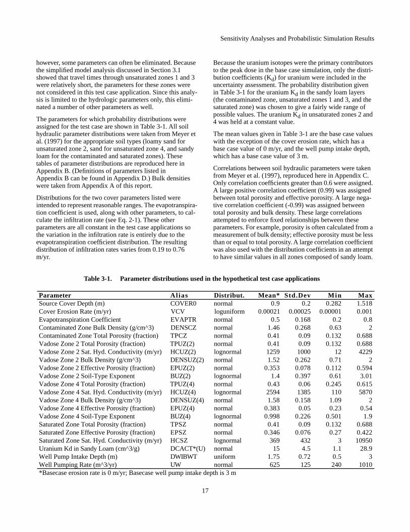
Sensitivity Analyses and Probabilistic Simulation Results
however, some parameters can often be eliminated. Because the simplified model analysis discussed in Section 3.1 showed that travel times through unsaturated zones 1 and 3 were relatively short, the parameters for these zones were not considered in this test case application. Since this analy-sis is limited to the hydrologic parameters only, this elimi-nated a number of other parameters as well.
The parameters for which probability distributions were assigned for the test case are shown in Table 3-1. All soil hydraulic parameter distributions were taken from Meyer et al. (1997) for the appropriate soil types (loamy sand for unsaturated zone 2, sand for unsaturated zone 4, and sandy loam for the contaminated and saturated zones). These tables of parameter distributions are reproduced here in Appendix B. (Definitions of parameters listed in Appendix B can be found in Appendix D.) Bulk densities were taken from Appendix A of this report.
Distributions for the two cover parameters listed were intended to represent reasonable ranges. The evapotranspira-tion coefficient is used, along with other parameters, to cal-culate the infiltration rate (see Eq. 2-1). These other parameters are all constant in the test case applications so the variation in the infiltration rate is entirely due to the evapotranspiration coefficient distribution. The resulting distribution of infiltration rates varies from 0.19 to 0.76 m/yr.
Because the uranium isotopes were the primary contributors to the peak dose in the base case simulation, only the distri-bution coefficients (Kd) for uranium were included in the uncertainty assessment. The probability distribution given in Table 3-1 for the uranium Kd in the sandy loam layers (the contaminated zone, unsaturated zones 1 and 3, and the saturated zone) was chosen to give a fairly wide range of possible values. The uranium Kd in unsaturated zones 2 and 4 was held at a constant value.
The mean values given in Table 3-1 are the base case values with the exception of the cover erosion rate, which has a base case value of 0 m/yr, and the well pump intake depth, which has a base case value of 3 m.
Correlations between soil hydraulic parameters were taken from Meyer et al. (1997), reproduced here in Appendix C. Only correlation coefficients greater than 0.6 were assigned. A large positive correlation coefficient (0.99) was assigned between total porosity and effective porosity. A large nega-tive correlation coefficient (-0.99) was assigned between total porosity and bulk density. These large correlations attempted to enforce fixed relationships between these parameters. For example, porosity is often calculated from a measurement of bulk density; effective porosity must be less than or equal to total porosity. A large correlation coefficient was also used with the distribution coefficients in an attempt to have similar values in all zones composed of sandy loam.
Table 3-1. Parameter distributions used in the hypothetical test case applications
Parameter Al ias Distribut. Mean* Std.Dev Min MaxSource Cover Depth (m) COVER0 normal 0.9 0.2 0.282 1.518Cover Erosion Rate (m/yr) VCV loguniform 0.00021 0.00025 0.00001 0.001Evapotranspiration Coefficient EVAPTR normal 0.5 0.168 0.2 0.8Contaminated Zone Bulk Density (g/cm^3) DENSCZ normal 1.46 0.268 0.63 2Contaminated Zone Total Porosity (fraction) TPCZ normal 0.41 0.09 0.132 0.688Vadose Zone 2 Total Porosity (fraction) TPUZ(2) normal 0.41 0.09 0.132 0.688Vadose Zone 2 Sat. Hyd. Conductivity (m/yr) HCUZ(2) lognormal 1259 1000 12 4229Vadose Zone 2 Bulk Density (g/cm^3) DENSUZ(2) normal 1.52 0.262 0.71 2Vadose Zone 2 Effective Porosity (fraction) EPUZ(2) normal 0.353 0.078 0.112 0.594Vadose Zone 2 Soil-Type Exponent BUZ(2) lognormal 1.4 0.397 0.61 3.01Vadose Zone 4 Total Porosity (fraction) TPUZ(4) normal 0.43 0.06 0.245 0.615Vadose Zone 4 Sat. Hyd. Conductivity (m/yr) HCUZ(4) lognormal 2594 1385 110 5870Vadose Zone 4 Bulk Density (g/cm^3) DENSUZ(4) normal 1.58 0.158 1.09 2Vadose Zone 4 Effective Porosity (fraction) EPUZ(4) normal 0.383 0.05 0.23 0.54Vadose Zone 4 Soil-Type Exponent BUZ(4) lognormal 0.998 0.226 0.501 1.9Saturated Zone Total Porosity (fraction) TPSZ normal 0.41 0.09 0.132 0.688Saturated Zone Effective Porosity (fraction) EPSZ normal 0.346 0.076 0.27 0.422Saturated Zone Sat. Hyd. Conductivity (m/yr) HCSZ lognormal 369 432 3 10950Uranium Kd in Sandy Loam (cm^3/g) DCACT*(U) normal 15 4.5 1.1 28.9Well Pump Intake Depth (m) DWIBWT uniform 1.75 0.72 0.5 3Well Pumping Rate (m^3/yr) UW normal 625 125 240 1010*Basecase erosion rate is 0 m/yr; Basecase well pump intake depth is 3 m
17

Sensitivity Analyses and Probabilistic Simulation Results
[Note, however, that the code used by RESRAD to generate realizations of parameter values (Iman and Shortencarier, 1984) may modify these correlations for computational rea-sons.]
3.3 Deterministic Sensitivity Measures
The simplest measure of the sensitivity of peak dose, D, to the value of a parameter, x, is
(3-1)
where A is the nominal set of parameters at which the sensi-tivities are evaluated. The partial derivative can be estimated from the nominal dose by modifying the value of x by a small amount and making a second calculation of dose. To make relative comparisons between parameters meaningful, the sensitivity is usually normalized,
(3-2)
where xA and DA are the nominal values of the parameter and the peak dose. An additional measure of sensitivity that includes the magnitude of the variation in the parameters is obtained by multiplying Eq. 3-1 by the standard deviation of the parameter.
(3-3)
Note that Eq. 3-3 was referred to in Meyer and Gee (1999) as a measure of the importance of the parameter to uncer-tainty in dose and can be used to define critical parameters.
3.3.1 Base Case Sensitivity Results
Sensitivity of the peak total dose evaluated at the base case parameter values was determined by slightly modifying the base case parameter values one at a time (for those parame-ters listed in Table 3-1) and running RESRAD to determine the resulting change in the dose. In most cases, the base case parameter values were modified by increasing them by approximately one-fourth of the difference between the base case and maximum values. Deterministic sensitivities were calculated for the in situ case only.
The base case sensitivities, calculated according to Eqs. 3-1 to 3-3, are listed in Table 3-2. The peak dose is most sensi-tive to the evapotranspiration coefficient, the uranium distri-bution coefficient in the sandy loam soils, and the well pumping rate. The peak dose is much less sensitive to the remaining parameters, although the cover erosion rate and the bulk density/total porosity/effective porosity of the unsaturated zones are more important than the remaining parameters. These results are consistent with the conclu-sions of Meyer and Gee (1999) in their general assessment
S D∂x∂
-------A
=
Sn
xA
DA------- D∂
x∂-------
A
⋅=
Sσ σxD∂x∂
-------A
⋅=
Table 3-2. Deterministic sensitivity results about the base case parameter values for the in situ case
Parameter S S n S ·σEvapotranspiration Coefficient -252.00 -1.10 -42.34Uranium Kd in Sandy Loam (cm^3/g) -5.70 -0.74 -25.65Well Pumping Rate (m^3/yr) -0.16 -0.86 -19.87Cover Erosion Rate (m/yr) 18000.00 0.00 4.50Vadose Zone 4 Effective Porosity (fraction) 50.96 0.17 2.55Vadose Zone 2 Bulk Density (g/cm^3) -7.50 -0.10 -1.97Vadose Zone 4 Total Porosity (fraction) 30.00 0.11 1.80Vadose Zone 4 Bulk Density (g/cm^3) 8.33 0.11 1.32Vadose Zone 2 Effective Porosity (fraction) 10.64 0.03 0.83Contaminated Zone Bulk Density (g/cm^3) 2.22 0.03 0.60Vadose Zone 4 Soil-Type Exponent 1.15 0.01 0.26Contaminated Zone Total Porosity (fraction) -2.88 -0.01 -0.26Vadose Zone 4 Sat. Hyd. Conductivity (m/yr) 0.00 0.00 -0.24Vadose Zone 2 Sat. Hyd. Conductivity (m/yr) 0.00 0.00 -0.22Vadose Zone 2 Soil-Type Exponent 0.34 0.00 0.13Source Cover Depth (m) -0.50 0.00 -0.10Vadose Zone 2 Total Porosity (fraction) 0.00 0.00 0.00Saturated Zone Total Porosity (fraction) 0.00 0.00 0.00Saturated Zone Effective Porosity (fraction) 0.00 0.00 0.00Saturated Zone Sat. Hyd. Conductivity (m/yr) 0.00 0.00 0.00Well Pump Intake Depth (m) 0.00 0.00 0.00
18

Sensitivity Analyses and Probabilistic Simulation Results
of the sensitivity of simplified dose assessment codes (such as DandD, RESRAD, and MEPAS). Note that dose is insen-sitive to the saturated zone parameters as a consequence of using the mass balance transport model of RESRAD.
The results in Table 3-2 show that Eqs. 3-2 and 3-3 provide similar estimates of the relative sensitivity of dose to the parameters. Eq. 3-3 may be preferred since it includes a measure of the magnitude of each parameter’s uncertainty and it avoids the situation that occurs here with the cover erosion rate. The sensitivity to the cover erosion rate is underestimated using Eq. 3-2 (because the nominal value is zero for this parameter). Nonetheless, the relative impor-tance of the parameters is consistent using Eqs. 3-2 and 3-3 for this application.
3.3.2 Conservative Case Sensitivity Results
As discussed in Meyer and Gee (1999) as well as other sources, one of the problems with a deterministic sensitivity analysis is it considers changes in only one parameter at a time and potentially evaluates the sensitivities about a sin-gle point (the base case in this application). In a study for the high-level radioactive waste repository performance assessment (NRC, 1999), these problems were addressed, in part, by performing a set of deterministic sensitivity analy-ses with the evaluation occurring about five points: a base case, a case with all parameters at their 90th percentile val-
ues, a case with all parameters at their 10th percentile val-ues, and two cases with parameter values chosen at random.
For the in situ test case application, a similar, but limited approach was taken. A second deterministic sensitivity anal-ysis was carried out with all parameters set to reasonably conservative values. For most parameters, the conservative values were (approximately) either the 25th or 75th percen-tiles of the distributions given in Table 3-1. Which of these two values was used was determined from physical under-standing of the models used in RESRAD or from the sensi-tivities evaluated at the base case parameter values (Table 3-2). A conservative set of parameters was chosen instead of, for example, a 90th percentile set because it was felt that evaluating the sensitivities with all parameters at conservative values would reveal any possible impact of parameter interactions in the region of concern (i.e., the region of large peak doses). Setting all parameters at large values (or small values) could result in a cancellation of sen-sitivities if one parameter has a negative effect on dose and another has a positive effect. Note that in choosing conser-vative values, physical conditions, such as the total porosity always being greater than or equal to the effective porosity, were maintained.
The results of the sensitivity measures evaluated at the con-servative parameter values are presented in Table 3-3. Note that the peak dose using the conservative parameter values was 398 mrem/yr and occurred at 516 years. As measured by Eq. 3-3, the largest sensitivity was to the uranium distri-
Table 3-3. Deterministic sensitivity results about the conservative parameter values for the in situ case
Parameter Basecase Conserv. S S n S ·σUranium Kd in Sandy Loam (cm^3/g) 15 9 -35.90 -0.81 -161.55Evapotranspiration Coefficient 0.5 0.28496 -470.61 -0.34 -79.06Well Pumping Rate (m^3/yr) 625 465 -0.46 -0.54 -57.50Vadose Zone 4 Bulk Density (g/cm^3) 1.58 1.78224 122.63 0.55 19.38Vadose Zone 2 Bulk Density (g/cm^3) 1.52 1.85536 63.22 0.29 16.56Vadose Zone 2 Effective Porosity (fraction) 0.353 0.45284 172.28 0.20 13.44Vadose Zone 4 Effective Porosity (fraction) 0.383 0.447 206.25 0.23 10.31Vadose Zone 4 Total Porosity (fraction) 0.43 0.45 -165.00 -0.19 -9.90Source Cover Depth (m) 0.9 0.1 -29.50 -0.01 -5.90Cover Erosion Rate (m/yr) 0 0.0005 21600.00 0.03 5.40Vadose Zone 4 Sat. Hyd. Conductivity (m/yr) 2594 1205.322 0.00 0.00 -2.18Contaminated Zone Bulk Density (g/cm^3) 1.46 1.80304 7.00 0.03 1.88Vadose Zone 4 Soil-Type Exponent 0.998 1.295941 7.32 0.02 1.66Vadose Zone 2 Sat. Hyd. Conductivity (m/yr) 1259 402.75 0.00 0.00 -1.51Contaminated Zone Total Porosity (fraction) 0.41 0.2948 -6.94 -0.01 -0.63Vadose Zone 2 Soil-Type Exponent 1.4 1.922789 1.36 0.01 0.54Vadose Zone 2 Total Porosity (fraction) 0.41 0.45 0.00 0.00 0.00Saturated Zone Total Porosity (fraction) 0.41 0.2948 0.00 0.00 0.00Saturated Zone Effective Porosity (fraction) 0.346 0.24872 0.00 0.00 0.00Saturated Zone Sat. Hyd. Conductivity (m/yr) 369 787.1481 0.00 0.00 0.00Well Pump Intake Depth (m) 3 3 0.00 0.00 0.00
19

Sensitivity Analyses and Probabilistic Simulation Results
bution coefficient value in the sandy loam soils. This sensi-tivity is due almost entirely to the distribution coefficient of the uranium isotopes in the contaminated zone only. The contaminated zone distribution coefficient determines the release of uranium from the source, which has a large impact on the peak dose for the test case application.
In addition to the distribution coefficient of uranium in the contaminated zone, the peak dose at the conservative parameter values is highly sensitive to the evapotranspira-tion coefficient and the well pumping rate. Peak dose is also sensitive to the porosities and bulk densities in the unsatur-ated zone layers, but to a lesser degree. These results are comparable to the sensitivities evaluated at the base case solution and indicate that the critical hydrologic parameters are consistent for both parameter sets.
3.4 Probabilistic Analyses
Probabilistic simulation of dose can be used to provide quantitative estimates of the uncertainty in dose due to parameter uncertainty. These estimates may be derived as a probability distribution of dose or as a mean and variance, depending on the method used. Probabilistic simulation
results can also be used to evaluate the sensitivity of dose to parameter values. The statistical sensitivity measures calcu-lated by RESRAD v. 6.0 are the partial (rank) correlation coefficients and partial (rank) regression coefficients. Multi-ple linear regression with stepwise addition or deletion of variables has also been used to determine parameter impor-tance (e.g., NRC, 1999), but is not implemented in RES-RAD.
For the hypothetical test cases, Monte Carlo simulation was used to derive the probability distribution of dose. The parameter distributions from Table 3-1 were input to the uncertainty analysis component of RESRAD v. 6.0 along with the parameter correlations discussed in Section 3.2. For the excavation case, the cover parameters were not used since there is no cover for this case. 100 realizations were used in each Monte Carlo simulation.
3.4.1 In Situ Case Results
The distributions of peak total dose from all pathways and the time of the peak dose for the Monte Carlo simulation of the in situ case are shown in Figure 3-2. The distributions are shown as a histogram and as an empirical cumulative
25
20
15
10
5
0
Num
ber
10
8
6
4
2
Num
ber
1.0
0.8
0.6
0.4
0.2
Em
piri
cal c
df
4003002001000Peak Dose (mrem/yr)
N = 100Min = 0Max = 488.7Mean = 120.48StDev = 78.317Median = 115.35
1.0
0.8
0.6
0.4
0.2
Em
piri
cal c
df
140012001000800600Time of Peak Dose (yr)
N = 100Min = 488.4Max = 1500Mean = 995.77StDev = 281.72Median = 950.7
Figure 3-2. Histogram (top) and empirical cdf (bottom) of peak dose (left) and the time of the peak dose (right) for the in situ test case Monte Carlo simulation
20

Sensitivity Analyses and Probabilistic Simulation Results
distribution function (cdf). Summary statistics are listed as well. The circular mark with error bars in the cdf plot indi-cates the mean dose/time plus and minus one standard devi-ations. The mean peak dose for this case (120 mrem/yr) is very similar to the base case peak dose (115 mrem/yr). This result cannot be expected in every case as the relationship between the peak dose and parameter values is often nonlin-ear and parameter distributions are frequently skewed. The standard deviation of peak dose (78 mrem/yr) is relatively large, resulting in a coefficient of variation of 0.65. The modeled parameter uncertainty thus is a significant contrib-utor to uncertainty in the peak dose for this case. Given the fact that the mean dose is almost five times the regulatory criterion, this level of uncertainty would deserve further investigation.
The histogram and cdf for the time to peak dose (shown in Figure 3-2) demonstrate that the uncertainty in this result is also significant. The mean time to peak (996 yr) is just under the regulatory criterion of 1000 yr. Since approxi-mately 10% of the 100 realizations had an actual peak dose that occurred later than 1500 years (the limit of this simula-tion), the mean time to peak (and the mean peak dose) would have been larger had the simulation been carried out for a sufficiently long time to reach each realization’s peak dose. Similarly, if this simulation had been limited to a 1000-year duration, the average peak dose would have been less than that given in Figure 3-2 since 40% of the parame-ter realizations resulted in a peak dose greater than 1000 years.
The deterministic analysis described in Section 3.3 evalu-ated sensitivities at a single point (the base case or conserva-tive case) and varied the parameters one at a time. Scatter plots of peak dose versus the parameter values used in the Monte Carlo simulation can reveal sensitivities over the entire range of parameter variation and can include the com-bined impact of multiple parameters on dose. A selection of scatter plots for the in situ case are shown in Figure 3-3. Of the parameters in the Monte Carlo simulation, the three that exhibited the most significant deterministic sensitivity were the evapotranspiration coefficient, the contaminated zone U-234 distribution coefficient, and the well pumping rate (see Tables 3-2 and 3-3). Relatively strong correlations with peak dose result from the Monte Carlo simulation results for these three parameters as well. Scatter plots for the cover erosion rate and bulk density of unsaturated zone 4 are also shown in Figure 3-3. These parameters had sensitivity coef-ficients that were small relative to the three dominant parameters, but were larger than for the other parameters. As seen in Figure 3-3, the cover erosion rate and the unsat-urated zone 4 bulk density do not produce a significant cor-relation with peak dose.
The statistical sensitivity measures calculated by RESRAD v.6.0 use the Monte Carlo results to estimate the impact on the dose of each individual parameter. These sensitivity
measures are reproduced in Table 3-4 for the peak total (all pathways) dose. The coefficient of determination for the partial correlation coefficient (PCC) and the standardized regression coefficient (SRC) was 0.79. For the measures using ranks (PRCC and SRRC), the coefficient of determi-nation was 0.84. The parameters are listed in Table 3-4 by rank according to the PRCC measure. The PRCC could rea-sonably be expected to best represent the importance of parameters because of the nonlinearities and parameter cor-relations in the simulation.
Three of the four statistical correlation measures show the evapotranspiration coefficient to be the most important parameter. There is little agreement between the various measures on the relative importance of the remaining parameters, however. The uranium distribution coefficients in the contaminated zone are ranked highly by the SRC measure, but not by the others (although the U-234 Kd in the contaminated zone is ranked third by the SRRC measure). The well pumping rate received a relatively low ranking from the regression coefficients. The cover depth is highly ranked by the PRCC measure only, but as shown in Figure 3-3 the peak dose does not appear to be strongly related to the cover depth. For this application it appears that, while the statistical correlation measures are useful in determining the relative importance of parameters, addi-tional analyses are required to be able to specify the critical parameters.
There are multiple measures of dose that could be used for comparison to the regulatory standard when probabilistic simulations are used in decommissioning analyses. One could use a statistic (such as the mean or the 50th percen-tile) of the distribution of peak dose. Peak dose as used here refers to the total (all pathways) dose occurring in the first 1000 years after decommissioning. This is the quantity used in Figures 3-2 and 3-3 (albeit without the 1000 year limit). An alternative measure of dose discussed in NRC (2000) is the peak of the mean dose, where the mean dose is calcu-lated as a function of time by averaging over all Monte Carlo realizations for each year of the simulation.
The mean total dose as a function of time is presented in Figure 3-4(A) for the in situ case. The median and 90th per-centile doses are shown in this figure as well. The base case dose as a function of time is presented for comparison. For the in situ test case, the mean dose at any time during the simulation is significantly less than the base case peak dose. This result occurs because of the sharp peak in the dose as a function of time and the fact that the parameter variation results in the time of the peak varying significantly. At any particular time, in fact, the fraction of realizations that have a dose greater than the 25 mrem/yr limit is quite small. Figure 3-4(B) illustrates this at times 500, 700, and 1000 years after decommissioning. At 1000 years, approximately 20% of the realizations result in a dose greater than 25 mrem. Figure 3-4(C) is a plot of peak dose versus the time
21

Sensitivity Analyses and Probabilistic Simulation Results
400
300
200
100
0
Peak
Dos
e (m
rem
/yr)
2 3 4 5 6 7
10-4
2 3 4 5 6 7
Cover Erosion Rate (m/yr)
400
300
200
100
0
Peak
Dos
e (m
rem
/yr)
0.70.60.50.40.3Evapotranspiration Coefficient
400
300
200
100
0
Peak
Dos
e (m
rem
/yr)
252015105Contaminated Zone U-234 Kd (cm
3/g)
400
300
200
100
0
Peak
Dos
e (m
rem
/yr)
1000900800700600500400Well Pumping Rate (m
3/yr)
400
300
200
100
0
Peak
Dos
e (m
rem
/yr)
1.21.00.80.6Cover Depth (m)
400
300
200
100
0
Peak
Dos
e (m
rem
/yr)
1.81.61.41.2Unsaturated Zone 4 Bulk Density (g/cm
3)
Figure 3-3. Scatter plots of peak dose versus parameter values for the in situ test case Monte Carlo simulation
22

Sensitivity Analyses and Probabilistic Simulation Results
Table 3-4. Statistical sensitivity measures for the in situ case (peak total dose) as calculated by RESRAD v. 6.0
Parameter Rank PCC Rank S R C Rank PRCC Rank S R R CEvapotranspiration coefficient 1 -0.8 4 -0.63 1 -0.87 1 -0.74Well pumping rate 2 -0.51 17 -0.29 2 -0.61 7 -0.32Cover depth 6 -0.24 24 -0.12 3 -0.39 11 -0.17Density of Unsaturated zone 4 21 -0.11 15 -0.31 4 -0.26 4 -0.4Effective Porosity of Unsaturated zone 4 28 0.08 19 0.21 5 0.24 5 0.38Cover erosion rate 27 0.08 30 0.04 6 0.24 17 0.1Total Porosity of Unsaturated zone 4 25 -0.09 10 -0.37 7 -0.23 2 -0.55Kd of U-234 in Contaminated Zone 8 -0.24 2 -0.86 8 -0.23 3 -0.46Well pump intake depth 29 -0.06 31 -0.03 9 -0.17 20 -0.07Kd of U-238 in Unsaturated Zone 1 16 -0.14 13 -0.34 10 0.11 13 0.14Saturated zone hydraulic conductivity 19 -0.12 28 -0.06 11 -0.11 25 -0.05Saturated zone effective porosity 15 -0.15 11 -0.35 12 -0.11 6 -0.32Density of Unsaturated zone 2 26 0.08 21 0.17 13 -0.1 12 -0.16Kd of U-238 in Saturated Zone 14 -0.15 9 -0.38 14 0.1 15 0.13Kd of U-238 in Contaminated Zone 11 0.17 3 0.83 15 -0.09 8 -0.21Kd of U-234 in Saturated Zone 22 0.11 18 0.21 16 0.07 18 0.08Density of contaminated zone 32 0.02 29 0.05 17 -0.06 9 -0.19Hydraulic Conductivity of Unsaturated zone 4 30 -0.04 32 -0.02 18 0.06 27 0.03Saturated zone total porosity 18 0.13 16 0.3 19 0.06 10 0.18Total Porosity of Unsaturated zone 2 23 0.11 12 0.34 20 -0.06 14 -0.14Kd of U-235 in Unsaturated Zone 3 7 -0.24 8 -0.46 21 -0.06 23 -0.05Kd of U-234 in Unsaturated Zone 3 24 0.1 22 0.17 22 -0.05 24 -0.05Kd of U-238 in Unsaturated Zone 3 10 -0.2 7 -0.5 23 0.05 22 0.06Effective Porosity of Unsaturated zone 2 13 -0.15 14 -0.33 24 0.05 19 0.07Kd of U-234 in Unsaturated Zone 1 20 0.11 20 0.21 25 0.05 26 0.05Kd of U-235 in Contaminated Zone 5 0.27 1 1.01* 26 0.04 21 0.07Contaminated zone total porosity 31 0.03 27 0.07 27 -0.04 16 -0.11Hydraulic Conductivity of Unsaturated zone 2 17 0.13 26 0.08 28 0.03 29 0.02b Parameter of Unsaturated zone 4 9 -0.21 23 -0.13 29 0.03 30 0.02Kd of U-235 in Saturated Zone 4 -0.28 5 -0.58 30 -0.03 28 -0.03b Parameter of Unsaturated zone 2 12 0.16 25 0.1 31 -0.03 31 -0.02Kd of U-235 in Unsaturated Zone 1 3 -0.3 6 -0.57 32 -0.01 32 -0.01P(R)CC: Partial (Rank) Correlation CoefficientS(R)RC: Standardized (Rank) Regression Coefficient
* Large, spurious SRC values will be generated by RESRAD v. 6.0 when strong correlations exist between input parameters (LePoire et al., 2000).
23

Sensitivity Analyses and Probabilistic Simulation Results
at which the peak occurs and illustrates the fact that the peak dose for the various realizations occurs over a broad range of times. (This result is also seen in Figure 3-2.)
3.4.2 Excavation Case Results
Probabilistic results for the excavation case are presented in a similar manner to those presented in the previous section for the in situ case. Figure 3-5 contains plots of the histo-grams and cumulative distribution functions for the peak
dose and the time of the peak dose. The distributions for this case are more highly skewed than for the in situ case, with a large number of realizations resulting in a peak dose near 11 mrem/yr that occurs at the beginning of the simulation. For these realizations, the peak dose is due to the external and water-independent pathways. Larger doses that occur later in time result from the transport of uranium isotopes through the groundwater. Approximately 20% of the realizations have a peak dose that occurs more than 1000 years after decommissioning. The mean dose is 15 mrem/yr with 13% of the realizations resulting in a peak dose greater than the
100
80
60
40
20
0
Tot
al D
ose
(mre
m/y
r)
1400120010008006004002000Time (yr)
Basecase 90th Percentile Mean Median
400
300
200
100
0
Peak
Dos
e (m
rem
/yr)
140012001000800600Time of Peak Dose (yr)
1.0
0.8
0.6
0.4
0.2
Em
piri
cal c
df
150100500Total Dose (mrem/yr)
Time = 500 yr Time = 700 yr Time = 1000 yr
Figure 3-4. (A) Total dose statistics as a function of time; (B) Total dose distributions at specified times; and (C) Peak dose vs. time of peak dose. All plots are for the in situ case.
(A)
(B) (C)
24

Sensitivity Analyses and Probabilistic Simulation Results
25 mrem/yr regulatory standard. The coefficient of variation for the peak dose is 51%. As with the in situ case, there is a significant amount of uncertainty in the peak dose and the time of the peak due to the modeled parameter uncertainty.
Statistical sensitivity measures as calculated by RESRAD v.6.0 are presented in Table 3-5 for the excavation case. These results were calculated using the peak total (all path-ways) dose. The coefficient of determination for the PCC and SRC measures was 0.80 and for the measures using ranks it was 0.81. As with the in situ case, the parameters are ordered in Table 3-5 by the magnitude of the partial rank correlation coefficient. The PRCC could reasonably be expected to best represent the importance of parameters because of the nonlinearities and parameter correlations in the simulation. As for the in situ case, however, the statisti-cal correlation measures do not provide a definitive ranking of the importance of parameters.
The saturated zone saturated hydraulic conductivity is highly ranked by each of the statistical correlation measures and appears to have the greatest impact on peak dose. The
evapotranspiration coefficient is highly ranked by the corre-lation coefficients, but not by the regression coefficients. The U-234 distribution coefficient in the contaminated zone is highly ranked by the regression coefficients. The impor-tance of the well pumping rate is estimated to be compara-tively low.
Scatter plots of peak dose as a function of parameter values are shown in Figure 3-6. The parameters chosen for plotting are the most sensitive parameters as measured by the statis-tical correlation measures. The dependence of peak dose on the saturated zone hydraulic conductivity is clear. A nonlin-ear relationship is implied. The scatter plots suggest a non-linear relationship between the peak dose and the U-234 distribution coefficient in the contaminated zone, although the relationship does not appear as strong, perhaps due to the confounding effect of other parameters (most notably the saturated zone hydraulic conductivity). From the remaining plots in Figure 3-6 it does not appear that the peak dose is very sensitive to the evapotranspiration coeffi-cient and the contaminated zone bulk density.
35
30
25
20
15
10
5
0
Num
ber
1.0
0.8
0.6
0.4
0.2
Em
piri
cal c
df
40302010Peak Dose (mrem/yr)
N = 100Min = 8.9Max = 49.07Mean = 15.467StDev = 7.9565Median = 11.755
40
30
20
10
0
Num
ber
1.0
0.8
0.6
0.4
0.2
Em
piri
cal c
df
12008004000Time of Peak Dose (yr)
N = 100Min = 0Max = 1500Mean = 574.11StDev = 528.77Median = 704.7
Figure 3-5. Histogram (top) and empirical cdf (bottom) of the peak dose (left) and the time of the peak dose (right) for the excavation test case Monte Carlo simulation
25

Sensitivity Analyses and Probabilistic Simulation Results
Scatter plots such as those in Figure 3-6 include the effect of varying multiple parameters at the same time. As a result, it is not easy to observe relatively weak relationships between peak dose and specific parameters. The saturated hydraulic conductivity in the saturated zone is the only parameter in this test case that has a sufficiently strong effect on peak dose to be obvious in the scatter plots. Statistical measures such as the partial (rank) correlation coefficient attempt to isolate the effect of individual parameters. As has been shown, however, these measures do not always agree and they may not make clear the relative importance of parame-ters. One additional analytical tool available is to examine the functional relationship between dose and a particular parameter using Monte Carlo simulation with a single
parameter varying. This can be conveniently accomplished using the built-in capabilities of RESRAD v. 6.0 (as well as other codes).
Examples of the results from single parameter Monte Carlo simulations are shown in Figure 3-7 for the saturated zone hydraulic conductivity, the evapotranspiration coefficient, and the U-234 distribution coefficient in the contaminated and saturated zones. These results were obtained with all parameters except for one at the excavation base case val-ues. These plots can be compared with those in Figure 3-6. The results provide additional evidence that the saturated zone hydraulic conductivity is much more important than the other parameters. In addition, it appears that the satu-
Table 3-5. Statistical sensitivity measures for the excavation case (peak total dose) as calculated by RESRAD v. 6.0
Parameter Rank PCC Rank S R C Rank PRCC Rank S R R CSaturated zone hydraulic conductivity 1 0.84 1 0.76 1 0.81 2 0.64Evapotranspiration coefficient 2 -0.38 17 -0.19 2 -0.27 13 -0.13Kd of U-234 in Unsaturated Zone 1 10 0.16 11 0.33 3 0.26 6 0.36Density of contaminated zone 7 0.19 5 0.56 4 0.25 1 0.74Kd of U-234 in Contaminated Zone 9 -0.17 2 -0.68 5 -0.22 3 -0.58Kd of U-238 in Saturated Zone 11 -0.16 12 -0.33 6 0.19 7 0.25Hydraulic Conductivity of Unsaturated zone 2 22 0.04 24 0.02 7 0.16 16 0.11Kd of U-234 in Unsaturated Zone 3 18 0.11 14 0.23 8 0.15 8 0.21Kd of U-238 in Contaminated Zone 8 0.17 3 0.67 9 -0.15 5 -0.39Kd of U-238 in Unsaturated Zone 1 15 -0.14 13 -0.28 10 0.14 9 0.2Contaminated zone total porosity 13 0.15 8 0.44 11 0.14 4 0.41Density of Unsaturated zone 4 30 0 30 0 12 -0.11 10 -0.18b Parameter of Unsaturated zone 2 28 0.01 29 0 13 0.11 19 0.09Well pumping rate 14 -0.15 19 -0.07 14 -0.1 27 -0.04Kd of U-234 in Saturated Zone 24 0.01 23 0.02 15 -0.08 18 -0.1Kd of U-235 in Unsaturated Zone 1 17 0.11 15 0.2 16 0.07 21 0.08Density of Unsaturated zone 2 26 -0.01 26 -0.01 17 0.07 15 0.11b Parameter of Unsaturated zone 4 25 -0.01 28 -0.01 18 0.07 23 0.06Kd of U-235 in Contaminated Zone 12 -0.15 6 -0.55 19 -0.07 11 -0.16Kd of U-238 in Unsaturated Zone 3 5 -0.2 9 -0.4 20 0.07 20 0.09Effective Porosity of Unsaturated zone 2 20 0.05 18 0.09 21 0.06 17 0.11Well pump intake depth 16 -0.14 20 -0.06 22 -0.05 28 -0.02Kd of U-235 in Saturated Zone 6 0.2 10 0.35 23 0.05 26 0.05Kd of U-235 in Unsaturated Zone 3 19 0.11 16 0.19 24 0.05 25 0.05Total Porosity of Unsaturated zone 4 29 0 27 0.01 25 -0.05 14 -0.11Saturated zone total porosity 3 0.25 4 0.59 26 0.04 12 0.14Effective Porosity of Unsaturated zone 4 27 0.01 25 0.02 27 0.04 22 0.06Hydraulic Conductivity of Unsaturated zone 4 21 -0.04 22 -0.02 28 0.03 29 0.02Total Porosity of Unsaturated zone 2 23 -0.02 21 -0.05 29 0.02 24 0.06Saturated zone effective porosity 4 -0.23 7 -0.55 30 0 30 -0.01P(R)CC: Partial (Rank) Correlation CoefficientS(R)RC: Standardized (Rank) Regression Coefficient
26

Sensitivity Analyses and Probabilistic Simulation Results
rated zone hydraulic conductivity has a threshold value, below which the dose is essentially constant and above which the dose is linearly related to the conductivity. With the remaining parameters at their base case values, that threshold is approximately 200 m/yr. This relationship com-pares well with the Monte Carlo results shown in Figure 3-6.
The evapotranspiration coefficient and the U-234 distribu-tion coefficient in the contaminated zone, two parameters that were highly ranked by the statistical measures, exhibit little influence on the peak dose with the remaining parame-ters at their base case values. In contrast, the U-234 distribu-tion coefficient in the saturated zone was not highly ranked by any of the statistical measures, but has a relatively large impact on peak dose according to Figure 3-7. It is possible that the combinations of parameter values used in the Monte Carlo simulation render this parameter less significant than
indicated here, but that determination would require addi-tional analyses.
Total dose statistics as a function of time are shown in Figure 3-8. The mean, median, and 90th percentile of total dose are shown along with the excavation base case dose as a function of time. As with the in situ case, the peak of the mean dose is less than the peak of the base case results, although for the excavation case they are both less than the regulatory standard. The interpretation of these results is similar to that for the in situ case. Peak doses for individual realizations that result from the transport of uranium iso-topes in groundwater are (1) larger than the mean dose at any particular time and (2) occur at different times for dif-ferent realizations [see Figures 3-8(B) and 3-8(C)].
40
30
20
10
Peak
Dos
e (m
rem
/yr)
252015105Contaminated Zone U-234 Kd (cm
3/g)
40
30
20
10
Peak
Dos
e (m
rem
/yr)
3 4 5 6100
2 3 4 5 61000
2
Saturated Zone Sat. Hydraulic Conductivity (m/yr)
40
30
20
10
Peak
Dos
e (m
rem
/yr)
0.70.60.50.40.3Evapotranspiration Coefficient
40
30
20
10
Peak
Dos
e (m
rem
/yr)
1.81.61.41.21.0Contaminated Zone Bulk Density (g/cm
3)
Figure 3-6. Scatter plots of peak dose versus parameter values for the excavation test case Monte Carlo simulation
27
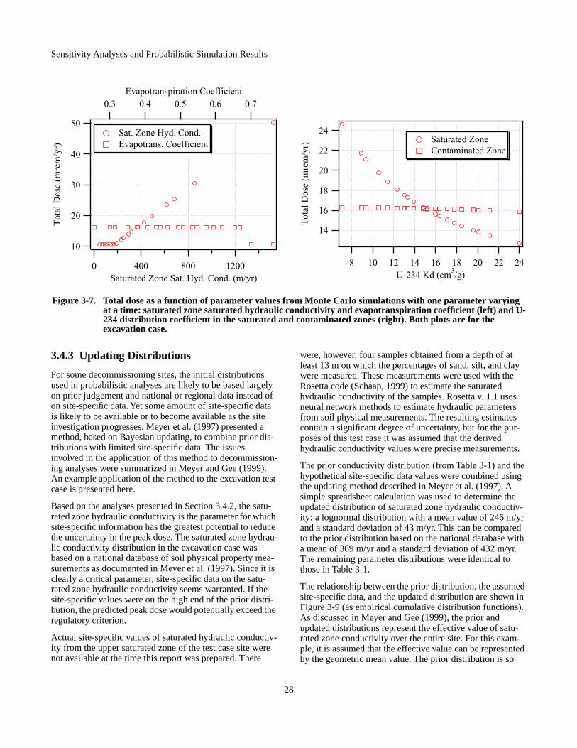
Sensitivity Analyses and Probabilistic Simulation Results
3.4.3 Updating Distributions
For some decommissioning sites, the initial distributions used in probabilistic analyses are likely to be based largely on prior judgement and national or regional data instead of on site-specific data. Yet some amount of site-specific data is likely to be available or to become available as the site investigation progresses. Meyer et al. (1997) presented a method, based on Bayesian updating, to combine prior dis-tributions with limited site-specific data. The issues involved in the application of this method to decommission-ing analyses were summarized in Meyer and Gee (1999). An example application of the method to the excavation test case is presented here.
Based on the analyses presented in Section 3.4.2, the satu-rated zone hydraulic conductivity is the parameter for which site-specific information has the greatest potential to reduce the uncertainty in the peak dose. The saturated zone hydrau-lic conductivity distribution in the excavation case was based on a national database of soil physical property mea-surements as documented in Meyer et al. (1997). Since it is clearly a critical parameter, site-specific data on the satu-rated zone hydraulic conductivity seems warranted. If the site-specific values were on the high end of the prior distri-bution, the predicted peak dose would potentially exceed the regulatory criterion.
Actual site-specific values of saturated hydraulic conductiv-ity from the upper saturated zone of the test case site were not available at the time this report was prepared. There
were, however, four samples obtained from a depth of at least 13 m on which the percentages of sand, silt, and clay were measured. These measurements were used with the Rosetta code (Schaap, 1999) to estimate the saturated hydraulic conductivity of the samples. Rosetta v. 1.1 uses neural network methods to estimate hydraulic parameters from soil physical measurements. The resulting estimates contain a significant degree of uncertainty, but for the pur-poses of this test case it was assumed that the derived hydraulic conductivity values were precise measurements.
The prior conductivity distribution (from Table 3-1) and the hypothetical site-specific data values were combined using the updating method described in Meyer et al. (1997). A simple spreadsheet calculation was used to determine the updated distribution of saturated zone hydraulic conductiv-ity: a lognormal distribution with a mean value of 246 m/yr and a standard deviation of 43 m/yr. This can be compared to the prior distribution based on the national database with a mean of 369 m/yr and a standard deviation of 432 m/yr. The remaining parameter distributions were identical to those in Table 3-1.
The relationship between the prior distribution, the assumed site-specific data, and the updated distribution are shown in Figure 3-9 (as empirical cumulative distribution functions). As discussed in Meyer and Gee (1999), the prior and updated distributions represent the effective value of satu-rated zone conductivity over the entire site. For this exam-ple, it is assumed that the effective value can be represented by the geometric mean value. The prior distribution is so
50
40
30
20
10
Tot
al D
ose
(mre
m/y
r)
12008004000Saturated Zone Sat. Hyd. Cond. (m/yr)
0.70.60.50.40.3Evapotranspiration Coefficient
Sat. Zone Hyd. Cond. Evapotrans. Coefficient
24
22
20
18
16
14
Tot
al D
ose
(mre
m/y
r)
24222018161412108U-234 Kd (cm
3/g)
Saturated Zone Contaminated Zone
Figure 3-7. Total dose as a function of parameter values from Monte Carlo simulations with one parameter varying at a time: saturated zone saturated hydraulic conductivity and evapotranspiration coefficient (left) and U-234 distribution coefficient in the saturated and contaminated zones (right). Both plots are for the excavation case.
28

Sensitivity Analyses and Probabilistic Simulation Results
much broader than the updated distribution because it assumes that there is no information at the site about the sat-urated zone hydraulic conductivity other than the textural characterization. As shown by the error bars in Figure 3-9 (representing plus or minus one standard deviation about the arithmetic mean value), the presence of actual site-specific measurements significantly reduces the uncertainty in the mean (effective) hydraulic conductivity. As a result of the reduction of the standard deviation, the arithmetic mean of the updated conductivity distribution is significantly smaller. The updated geometric mean, however, is little changed.
The effect of the updated saturated zone hydraulic conduc-tivity on the peak dose was determined by repeating the Monte Carlo simulation with the new (updated) hydraulic conductivity distribution. The resulting cumulative distribu-tion functions for the peak dose are shown in Figure 3-10. As a result of the smaller average hydraulic conductivity, there is a small reduction in the mean of the updated peak dose. More significantly, the coefficient of variation of the peak dose is reduced from 51% to 33% and the percentage of realizations exceeding 25 mrem/yr is reduced from 13% to 2%. There were only minor changes in the distribution of the time of the peak dose.
16
14
12
10
8
6
4
Tot
al D
ose
(mre
m/y
r)
1400120010008006004002000Time (yr)
Basecase 90th Percentile Mean Median
1.0
0.8
0.6
0.4
0.2
Em
piri
cal c
df
40302010Total Dose (mrem/yr)
Time = 500 yr Time = 700 yr Time = 1000 yr
40
30
20
10
Peak
Dos
e (m
rem
/yr)
12008004000Time of Peak Dose (yr)
Figure 3-8. (A) Total dose statistics as a function of time; (B) Total dose distributions at specified times; and (C) Peak dose vs. time of peak dose. All plots are for the excavation case.
(A)
(B) (C)
29

Sensitivity Analyses and Probabilistic Simulation Results
The observed decrease in the variance of the peak dose as a result of updating the input parameter distribution(s) with site-specific data is a general result that can be expected to occur unless the updated parameter distribution has a larger variance than the prior distribution. The observed decrease in the mean of the updated peak dose distribution, on the
other hand, is a particular result of this test case application and should not be construed as a general conclusion. Had the site-specific hydraulic conductivity values used in the updating procedure been larger, the mean of the updated peak dose distribution could easily have been larger than the prior mean value.
1.0
0.8
0.6
0.4
0.2
0
Em
piri
cal c
df
2000150010005000Saturated Zone Hydraulic Conductivity (m/yr)
PriorN = 100Min = 22.422Max = 2227.3Mean = 361.32StDev = 373.03Median = 241.04
Prior Updated Site-Specific Data
UpdatedN = 100Min = 155.22Max = 368.19Mean = 245.86StDev = 42.673Median = 242.48
Figure 3-9. Prior and updated probability distributions of the saturated zone hydraulic conductivity for the excavation case. Site-specific data values used in the updating procedure are shown as well.
1.0
0.8
0.6
0.4
0.2
0
Em
piri
cal c
df
40302010Peak Dose (mrem/yr)
PriorN = 100Min = 8.9Max = 49.07Mean = 15.467StDev = 7.9565Median = 11.755
Prior Updated
UpdatedN = 100Min = 8.9Max = 37.3Mean = 13.077StDev = 4.265Median = 11.76
Figure 3-10. Prior and updated probability distributions of the peak dose for the excavation case. The updated distribution uses the updated saturated zone hydraulic conductivity distribution with the remaining parameter distributions taken from Table 3-1.
30

4 Conclusions
This report is a follow-on report to NUREG/CR-6656 (Meyer and Gee, 1999) and has illustrated the application of many of the methods discussed there using hypothetical decommissioning test cases. The source term and scenarios for the test cases were based on an actual decommissioning case and the physical setting was based on the site of a field experiment carried out in Arizona. Basic soil and climate information from the site were used in the application. The soil profile was simplified from the site-specific information to reduce the computational requirements of the simulations and to fit the simplified conceptual models of the codes used.
A series of deterministic simulations were carried out using the codes DandD v. 1.0 and RESRAD v. 6.0. DandD was executed with the test case source term and all default parameter values. This screening case resulted in a peak dose of 829 mrem/yr. The DandD code was also run with site-specific parameters. A peak dose of 285 mrem/yr was obtained with most of the physical hydrologic parameters modified to reflect site-specific conditions. With default hydrologic parameters and modified distribution coeffi-cients, the peak dose was 198 mrem/yr. With site-specific hydrologic parameters and modified distribution coeffi-cients, the peak dose from DandD was 70 mrem/yr.
Several deterministic simulations using RESRAD were car-ried out also using best-estimate (base case) parameter val-ues. The base case parameters were based on national databases and information from the site in Arizona. The in situ case modeled the waste in its original buried location and assumed that a cover was in place. The in situ case resulted in a peak dose of 115 mrem/yr. An excavation case was also simulated in which the waste was assumed to have been excavated and widely spread about in a surface soil mixture. This case more closely resembled the DandD con-ceptual model. The RESRAD excavation base case resulted in a peak dose of 16 mrem/yr.
A variety of deterministic sensitivity analyses were applied to the test cases, including a simplified model implemented in a spreadsheet, standard sensitivity measures, and applica-tion of sensitivity analysis to the base case and a conserva-tive parameter case. For the in situ test case, these analyses indicated that the evapotranspiration coefficient and the ura-nium distribution coefficients were the most important parameters contributing to the uncertainty in peak dose. The well pumping rate was also important. Soil hydraulic parameters were much less important. Deterministic sensi-tivity analyses were not carried out for the excavation case.
Probabilistic analyses were carried out for the in situ and excavation test cases using the Monte Carlo simulation
capability of RESRAD. Results were presented as distribu-tions for the peak total dose and the time of the peak dose. Statistics for the total dose as a function of time were also presented. Uncertainties in the peak dose and the time of the peak dose were significant with the coefficient of variation for the peak dose exceeding 50% in both cases. Several measures of sensitivity based on the probabilistic results were also discussed. These included scatter plots of peak dose versus parameter values, statistical sensitivity mea-sures calculated by RESRAD, and single-parameter Monte Carlo simulations to clarify the relationship between dose and critical parameter values. No single measure was a reli-able indicator of the relative importance of the parameters. The greatest value from an uncertainty analysis can be obtained by using multiple analytical methods and graphical presentations.
The Monte Carlo simulation results were also used to obtain the mean total dose as a function of time. The peak of this mean is an alternative comparative measure being consid-ered for decommissioning analyses. For the test cases con-sidered here, the mean dose at any time during the simulation was significantly less than the base case peak doses (and significantly less than the mean of the peak dose distributions). This result occurred because of the sharp peak in the dose as a function of time and the fact that the parameter variation resulted in the time of the peak varying significantly.
A method to update parameter probability distributions was applied to the excavation test case. Based on the statistical sensitivity analyses, the saturated zone hydraulic conductiv-ity was the most critical parameter for this case. Because site-specific measurements were not available for this parameter, data was generated using four measurements of physical properties from the deepest samples available at the test case site. The standard deviation of the saturated zone hydraulic conductivity was significantly reduced by including the site-specific values. When the updated satu-rated zone hydraulic conductivity distribution was applied to the excavation case, the geometric mean of the peak dose was little changed, but the coefficient of variation of the peak dose was reduced from 51% to 33% and the percent-age of realizations exceeding 25 mrem/yr was reduced from 13% to 2%. It was noted that the updating procedure makes a number of assumptions about the distributions involved and also assumes that the site-specific data is error-free, an assumption that underestimates parameter uncertainty. Additional research is needed to establish general guidance for application of the updating method to decommissioning analyses.
31


5 References
Beyeler, W. E., W. A. Hareland, F. A Duran, T. J. Brown, E. Kalinina, D. P. Gallegos, and P. A. Davis, “Residual Radio-active Contamination from Decommissioning: Parameter Analysis,” Draft Report for Comment, NUREG/CR-5512, Vol. 3, October, 1999, Sandia National Laboratories, Albu-querque, NM, 1999.
Campbell, G. S., “A simple method for determining unsatur-ated conductivity from moisture retention data,” Soil Sci., 117:311-314, 1974.
Cole, C. R., M. D. Williams, W. A. Perkins, M. D. White, and P. D. Meyer, “Groundwater Models in Support of NUREG/CR-5512,” NUREG/CR-5621, U.S. Nuclear Regu-latory Commission, Washington, DC, 1998.
Kennedy, J.D., and D.L. Strenge, “Residual Radioactive Contamination from Decommissioning: Technical Basis for Translating Contamination Levels to Annual Total Effective Dose Equivalent,” NUREG/CR-5512, (PNL-7994), U.S. Nuclear Regulatory Commission, Washington, D.C., 1992.
Federal Register, “10 CFR Part 20 et al., Radiological Crite-ria for License Termination; Final Rule,” Vol. 62, No. 139, Monday, July 21, pp. 39058-39092, 1997.
Helton, J. C., “Uncertainty and Sensitivity Analysis Tech-niques for Use in Performance Assessment for Radioactive Waste Disposal,” Reliability Engineering and System Safety, 42:327-367, 1993.
Iman, R. L. and M. J. Shortencarier, “A FORTRAN 77 Pro-gram and User’s Guide for the Generation of Latin Hyper-cube and Random Samples for Use with Computer Models,” NUREG/CR-3624, SAND83-2365, U.S. Nuclear Regulatory Commission, Washington, D.C., 1984
Kennedy, J.D., and D.L. Strenge, “Residual Radioactive Contamination from Decommissioning: Technical Basis for Translating Contamination Levels to Annual Total Effective Dose Equivalent,” NUREG/CR-5512, (PNL-7994), U.S. Nuclear Regulatory Commission, Washington, D.C., 1992.
Kozak, M. W., N.E. Olague, R. R. Rao, and J. T. McCord, “Evaluation of a Performance Assessment Methodology for Low-Level Radioactive Waste Disposal Facilities,” NUREG/CR-5927, Vol. 1, U. S. Nuclear Regulatory Com-mission, Washington, D.C., 1993.
LePoire, D., J. Arnish, E. Gnanapragasam, S. Kamboj, B. M. Biwer, J.-J. Cheng, C. Yu, and S. Y. Chen, “Probabilistic Modules for the RESRAD and RESRAD-BUILD Computer Codes,” NUREG/CR-6692, U.S. Nuclear Regulatory Com-mission, Washington, D.C., 2000.
Meyer, P. D. and G. W. Gee, “Information on Hydrologic Conceptual Models, Parameters, Uncertainty Analysis, and Data Sources for Dose Assessments at Decommissioning Sites,” NUREG/CR-6656, U.S. Nuclear Regulatory Com-mission, Washington, D.C., 1999.
Meyer, P.D., M.L. Rockhold, and G.W. Gee, “Uncertainty Analyses of Infiltration and Subsurface Flow and Transport for SDMP Sites,” NUREG/CR-6565, U.S. Nuclear Regula-tory Commission, Washington, DC, 1997.
Morgan, M. G. and M. Henrion, Uncertainty: A Guide to Dealing with Uncertainty in Quantitative Risk and Policy Analysis, Cambridge University Press, New York, 332 pp., 1990.
NRC, “Standard Review Plan for Decommissioning,” NUREG-1727, U.S. Nuclear Regulatory Commission, Washington, D.C., 2000.
NRC, “NRC Sensitivity and Uncertainty Analyses for a Pro-posed HLW Repository at Yucca Mountain, Nevada, Using TPA 3.1,” NUREG-1668, Vol. 2, U.S. Nuclear Regulatory Commission, Washington, D.C., 1999.
NRC, “Decision Methods for Dose Assessments to Comply with Radiological Criteria for License Termination,” Draft NUREG-1549, U.S. Nuclear Regulatory Commission, Washington, D.C., February 3, 1998.
Robson, S. G. and E. R. Banta, “Groundwater Atlas of the United States, Segment 2: Arizona, Colorado, New Mexico, Utah,” Hydrologic Investigations Atlas 730-C, U.S. Geolog-ical Survey, 1995.
Schaap, M., Rosetta Version 1.1, 1999. Available at http://www.ussl.ars.usda.gov.
Sheppard, M. I. and D. H. Thibault, “Default Soil Solid/Liq-uid Partition Coefficients, Kds, for Four Major Soil Types: A Compendium,” Health Physics, 59(4):471-482, 1990.
Soil Survey Staff, National Characterization Data, Soil Sur-vey Laboratory, National Soil Survey Center, Natural Resources Conservation Service, Lincoln, NE, 1994.
Streile, G. P., K.D. Shields, J. L. Stroh, L. M. Bagaasen, G. Whelan, J. P. McDonald, J. G. Droppo, and J. W. Buck, “The Multimedia Environmental Pollutant Assessment Sys-tem (MEPAS): Source-Term Release Formulations,” PNNL-11248, Pacific Northwest National Laboratory, Richland, WA, 1996.
Wernig, M. A., A. M. Tomasi, F. A Duran, and C. D. Upde-graff, “Residual Radioactive Contamination from Decom-missioning, User’s Manual, Draft Report,” NUREG/CR-5512, Volume 2 (Draft), Sandia National Laboratories, May, 1999.
Whelan, G., J. P. McDonald, and C. Sato, “Multimedia Environmental Pollutant Assessment System (MEPAS): Groundwater Pathway Formulations,” PNNL-10907, Pacific Northwest National Laboratory, Richland, WA, 1996.
Young, M. H., P. J. Wierenga, A. W. Warrick, L. L. Hof-mann, S. A. Musil, M. Yao, C. J. Mai, Z. Zou, and B. R. Scanlon, “Results of Field Studies at the Maricopa Environ-
33

References
mental Monitoring Site, Arizona,” NUREG/CR-5694, U.S. Nuclear Regulatory Commission, Washington, D.C., 1999.
Yu, C., A. J. Zielen, J.-J. Cheng, Y. C. Yuan, L. G. Jones, D. J. LePoire, Y.Y Wang, C. O. Loureiro, E. Gnanapragasam, E. Faillace, A. Wallo III, W. A. Williams, and H. Peterson, “Manual for Implementing Residual Radioactive Material Guidelines Using RESRAD, Version 5.0,” ANL/EAD/LD-2, Argonne National Laboratory, Argonne, IL, 1993.
34

Appendix A: Recommended Soil Bulk Density Distributions
Dry soil bulk density data were obtained from the U.S. Nat-ural Resources Conservation Service Soil Characterization Database, dated May 1994. The data were divided accord-ing to USDA soil textural class based on the sand, silt, and clay percentages. The distribution of these data over textural classes can be seen in Figure 5-5 of NUREG/CR-6656 (Meyer and Gee, 1999).
For each textural class, the Kolmogorov-Smirnov D-statistic was calculated using hypothetical normal and lognormal distributions. The parameters for the hypothetical normal and lognormal distributions were based on the data. In all cases the D-statistic from the normal distribution was smaller than that from the lognormal distribution. In addi-tion, plots of the bulk density histogram for each soil texture were examined and appeared to better fit a normal distribu-tion. For these reasons, the normal distribution is recom-mended for modeling bulk density.
The mean and standard deviation of the bulk density data are given in the table below. These values reflect the elimi-nation of outliers from the dataset for each textural class. Outliers were defined as those points outside the mean plus
or minus four times the standard deviation, where the mean and standard deviation were calculated as the sample mean and sample standard deviation with the potential outliers eliminated. The upper and lower limits given in the table are the actual limits of the data extracted from the Soil Charac-terization Database. Samples with a bulk density less than 0.5 g/cm3 or greater than 2.0 g/cm3 were not included in the analysis.
Bulk density is highly correlated to saturated water content and effective porosity with correlations generally between -0.95 and -0.99.
A.1 ReferencesMeyer, P.D. and G.W. Gee, “Information on Hydrologic Conceptual Models, Parameters, Uncertainty Analysis, and Data Sources for Dose Assessments at Decommissioning Sites,” NUREG/CR-6656, U.S. Nuclear Regulatory Com-mission, Washington, DC, 1999.
Table A-1. Recommended parameters of normal distributions for bulk density
Soil Texture Number of Samples Mean Std. Deviation Lower Limit Upper Limit
Sand 811 1.578 0.158 1.0 1.99
Loamy Sand 1889 1.515 0.262 0.5 2.0
Sandy Loam 7195 1.461 0.268 0.5 2.0
Sandy Clay Loam 2189 1.518 0.186 0.76 2.0
Loam 5198 1.418 0.240 0.54 1.99
Silt Loam 6411 1.366 0.227 0.5 1.99
Silt 195 1.330 0.202 0.63 1.74
Clay Loam 3396 1.410 0.197 0.63 2.0
Silty Clay Loam 3139 1.405 0.148 0.8 1.91
Sandy Clay 386 1.491 0.177 0.87 1.94
Silty Clay 2165 1.37 0.154 0.73 1.82
Clay 4539 1.292 0.177 0.58 1.9
A-1


Appendix B: Recommended Soil Parameter Distributions
Probability distributions of three types (normal, lognormal, and beta) were used to approximate the soil hydraulic param-eter distributions generated from the Carsel and Parrish (1988) statistics. This appendix provides a summary of these distributions and presents tables of recommended dis-tributions for selected soil hydraulic parameters. The infor-mation provided in Sections B.1 – B.3 can be found in many good probability or statistics textbooks (e.g., Ang and Tang, 1975). Definitions of parameters can be found in Appendix D.
This appendix was originally presented in NUREG/CR-6565 (Meyer et al., 1997).
B.1 The Normal Distribution
The normal distribution has a density function given by
(B-1)
where x is the soil parameter being modeled and and are the parameters of the distribution. The mean, µ, and the variance, σ2, are related to the parameters of the normal dis-tribution as follows.
(B-2)
(B-3)
Although the normal distribution is unbounded, soil param-eters modeled by a normal distribution often have physical limits. These limits can be enforced by specifying that the soil parameter values fall between given quantiles of the normal distribution. In the tables below, the lower (A) and upper (B) limits of each normal distribution are the 0.001 and 0.999 quantiles calculated as follows.
(B-4)
B.2 The Lognormal distribution
The lognormal distribution has a density function given by
(B-5)
where γ and ζ are the parameters of the distribution. The mean and variance of the lognormal distribution are related to the parameters as follows.
(B-6)
(B-7)
These relationships can also be inverted.
(B-8)
(B-9)
The lognormal distribution is thus completely specified by either its parameters or its mean and variance.
The lognormal distribution is bounded below by zero, but has no upper bound. In the tables below, the lower and upper bound for the lognormal distributions are the 0.001 and 0.999 quantiles calculated as follows.
(B-10)
B.3 The Beta Distribution
The beta distribution has a density function given by
(B-11)
where q and r are parameters controlling the shape of the dis-tribution and A and B are the lower and upper limits of the distribution. β(q,r) is the beta function, calculated through its relationship to the gamma function.
(B-12)
where Γ( ) indicates the gamma function.
The mean and variance of the beta distribution are related to the parameters as follows.
(B-13)
(B-14)
With some algebraic manipulation, these relationships can be inverted to provide the shape parameters as a function of the mean, variance, and limits.
(B-15)
(B-16)
The beta distribution can thus be completed specified by its lower and upper limits and either its mean and variance or its shape parameters.
In the tables below, the lower and upper limits for the beta distributions are the actual limits, A and B.
f x( ) 1
2πσ'--------------- 1
2--- x µ'–
σ'-------------
2exp=
µ' σ'
µ µ'=
σ2 σ'2=
A µ' 3.09σ'–= B µ' 3.09σ'+=
f x( ) 1
2πζx----------------- 1
2--- x( )ln γ–
ζ----------------------
2exp=
µ γ 12---ζ2+( )exp=
σ2 µ2 ζ2( )exp 1–[ ]=
γ µln 12---ζ2–=
ζ σ2
µ2----- 1+
ln=
A γ 3.09ζ–( )exp= B γ 3.09ζ+( )exp=
f x( ) 1β q r,( )---------------- x A–( )q 1– B x–( )r 1–
B A–( )q r 1–+---------------------------------------------------=
β q r,( ) Γ q( )Γ r( )Γ q r+( )-----------------------=
µ Aq
q r+----------- B A–( )+=
σ2 qr
q r+( )2 q r 1+ +( )--------------------------------------------- B A–( )2=
q B µ–( ) µ A–( )σ2
------------------------------------ 1– µ A–
B A–-------------
=
r qB µ–µ A–-------------
=
B-1

Recommended Soil Parameter Distributions
B.4 Recommended Probability Distributions for Soil Hydraulic Parameters by Soil Texture
Tables B-1 to B-12 contain the recommended distributions for the selected soil hydraulic parameters. Each table repre-sents a particular USDA soil textural classification. Observed correlations between parameters are given in Appendix B.
Table B-1. Recommended distributions for Sand
Parameter Distribution1 Mean Std. Deviation Lower Limit2 Upper Limit2
θs Normal 0.430 0.0600 0.245 0.615
θr LN(-3.09,0.224)* 0.0466 0.0106 0.0228 0.0907
pe Normal 0.383 0.0610 0.195 0.572
fc LN(-2.83,0.241) 0.0607 0.0150 0.0280 0.124
wp LN(-3.09,0.224) 0.0466 0.0106 0.0227 0.0907
awc LN(-4.34,0.387) 0.0141 6.12E-03 3.95E-03 0.0431
α [cm-1] Normal 0.147 0.0255 0.0687 0.226
n LN(0.978,0.0998)* 2.67 0.267 1.95 3.62
hb LN(1.93,0.183) 7.02 1.38 3.92 12.1
λ LN(0.502,0.161) 1.67 0.267 1.00 2.72
b LN(-0.0253,0.216) 0.998 0.226 0.501 1.90
Ks [cm/s] Beta(1.398,1.842) 8.22E-03 4.39E-03 3.50E-04 0.0186
Table B-2. Recommended distributions for Loamy Sand
Parameter Distribution1 Mean Std. Deviation Lower Limit2 Upper Limit2
θs Normal 0.410 0.0900 0.132 0.688
θr Normal 0.0569 0.0145 0.0121 0.102
pe Normal 0.353 0.0913 0.0711 0.635
fc LN(-2.55,0.281) 0.0809 0.0224 0.0327 0.186
wp Normal 0.0570 0.0146 0.0119 0.102
awc LN(-3.85,0.491) 0.0239 0.0125 4.65E-03 0.0966
α [cm-1] Normal* 0.125 0.0404 2.03E-04 0.250
n LN(0.816,0.0910) 2.27 0.209 1.71 3.00
hb LN(2.15,0.401) 9.58 8.59 2.48 29.5
λ LN(0.226,0.164) 1.27 0.209 0.756 2.08
b LN(0.305,0.258) 1.40 0.397 0.610 3.01
Ks [cm/s] Beta(0.7992,1.910) 3.99E-03 3.17E-03 3.90E-05 0.0134
B-2
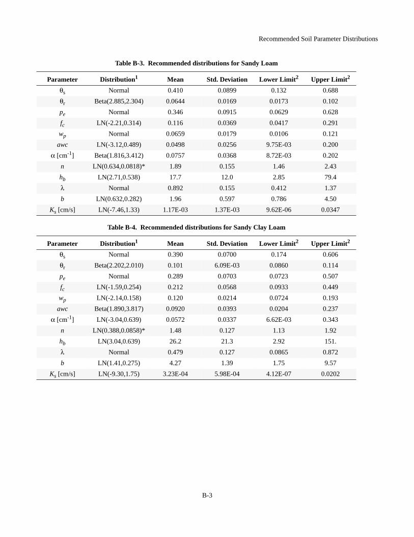
Recommended Soil Parameter Distributions
imit2
8
2
8
1
1
0
2
3
4
7
0
47
imit2
6
4
7
9
3
7
3
2
.
2
7
02
Table B-3. Recommended distributions for Sandy Loam
Parameter Distribution1 Mean Std. Deviation Lower Limit2 Upper L
θs Normal 0.410 0.0899 0.132 0.68
θr Beta(2.885,2.304) 0.0644 0.0169 0.0173 0.10
pe Normal 0.346 0.0915 0.0629 0.62
fc LN(-2.21,0.314) 0.116 0.0369 0.0417 0.29
wp Normal 0.0659 0.0179 0.0106 0.12
awc LN(-3.12,0.489) 0.0498 0.0256 9.75E-03 0.20
α [cm-1] Beta(1.816,3.412) 0.0757 0.0368 8.72E-03 0.20
n LN(0.634,0.0818)* 1.89 0.155 1.46 2.4
hb LN(2.71,0.538) 17.7 12.0 2.85 79.
λ Normal 0.892 0.155 0.412 1.3
b LN(0.632,0.282) 1.96 0.597 0.786 4.5
Ks [cm/s] LN(-7.46,1.33) 1.17E-03 1.37E-03 9.62E-06 0.03
Table B-4. Recommended distributions for Sandy Clay Loam
Parameter Distribution1 Mean Std. Deviation Lower Limit2 Upper L
θs Normal 0.390 0.0700 0.174 0.60
θr Beta(2.202,2.010) 0.101 6.09E-03 0.0860 0.11
pe Normal 0.289 0.0703 0.0723 0.50
fc LN(-1.59,0.254) 0.212 0.0568 0.0933 0.44
wp LN(-2.14,0.158) 0.120 0.0214 0.0724 0.19
awc Beta(1.890,3.817) 0.0920 0.0393 0.0204 0.23
α [cm-1] LN(-3.04,0.639) 0.0572 0.0337 6.62E-03 0.34
n LN(0.388,0.0858)* 1.48 0.127 1.13 1.9
hb LN(3.04,0.639) 26.2 21.3 2.92 151
λ Normal 0.479 0.127 0.0865 0.87
b LN(1.41,0.275) 4.27 1.39 1.75 9.5
Ks [cm/s] LN(-9.30,1.75) 3.23E-04 5.98E-04 4.12E-07 0.02
B-3
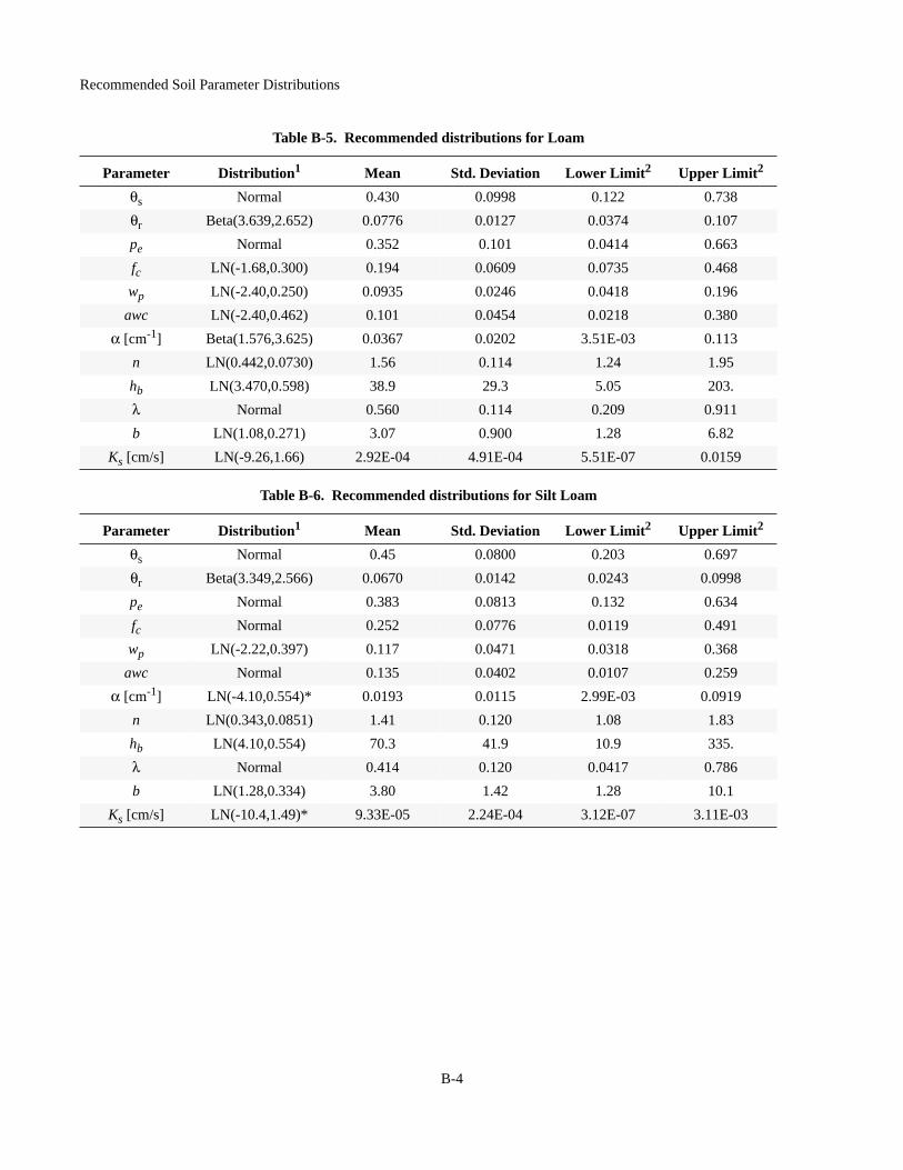
Recommended Soil Parameter Distributions
m
ower Limit2 Upper Limit2
0.122 0.738
0.0374 0.107
0.0414 0.663
0.0735 0.468
0.0418 0.196
0.0218 0.380
3.51E-03 0.113
1.24 1.95
5.05 203.
0.209 0.911
1.28 6.82
5.51E-07 0.0159
am
ower Limit2 Upper Limit2
0.203 0.697
0.0243 0.0998
0.132 0.634
0.0119 0.491
0.0318 0.368
0.0107 0.259
2.99E-03 0.0919
1.08 1.83
10.9 335.
0.0417 0.786
1.28 10.1
3.12E-07 3.11E-03
Table B-5. Recommended distributions for Loa
Parameter Distribution1 Mean Std. Deviation L
θs Normal 0.430 0.0998
θr Beta(3.639,2.652) 0.0776 0.0127
pe Normal 0.352 0.101
fc LN(-1.68,0.300) 0.194 0.0609
wp LN(-2.40,0.250) 0.0935 0.0246
awc LN(-2.40,0.462) 0.101 0.0454
α [cm-1] Beta(1.576,3.625) 0.0367 0.0202
n LN(0.442,0.0730) 1.56 0.114
hb LN(3.470,0.598) 38.9 29.3
λ Normal 0.560 0.114
b LN(1.08,0.271) 3.07 0.900
Ks [cm/s] LN(-9.26,1.66) 2.92E-04 4.91E-04
Table B-6. Recommended distributions for Silt Lo
Parameter Distribution1 Mean Std. Deviation L
θs Normal 0.45 0.0800
θr Beta(3.349,2.566) 0.0670 0.0142
pe Normal 0.383 0.0813
fc Normal 0.252 0.0776
wp LN(-2.22,0.397) 0.117 0.0471
awc Normal 0.135 0.0402
α [cm-1] LN(-4.10,0.554)* 0.0193 0.0115
n LN(0.343,0.0851) 1.41 0.120
hb LN(4.10,0.554) 70.3 41.9
λ Normal 0.414 0.120
b LN(1.28,0.334) 3.80 1.42
Ks [cm/s] LN(-10.4,1.49)* 9.33E-05 2.24E-04
B-4

Recommended Soil Parameter Distributions
Table B-7. Recommended distributions for Silt
Parameter Distribution1 Mean Std. Deviation Lower Limit2 Upper Limit2
θs Normal 0.456 0.110 0.1206 0.799
θr Beta(1.717,1.072) 0.0352 8.97E-03 0.0131 0.0490
pe Normal 0.425 0.110 0.0839 0.766
fc Normal 0.236 0.0578 0.0575 0.415
wp LN(-2.46,0.295) 0.0890 0.0268 0.0342 0.212
awc Normal 0.147 0.0395 0.0252 0.269
α [cm-1] Normal* 0.0178 5.73E-03 3.91E-05 0.0355
n Normal* 1.38 0.0369 1.27 1.49
hb LN(4.10,0.403) 68.1 74.8 17.3 209.
λ Normal 0.380 0.0369 0.266 0.494
b LN(1.16,0.140) 3.21 0.465 2.06 4.89
Ks [cm/s] LN(-10.0,0.475)* 4.89E-05 2.76E-05 9.95E-06 1.87E-04
Table B-8. Recommended distributions for Clay Loam
Parameter Distribution1 Mean Std. Deviation Lower Limit2 Upper Limit2
θs Normal 0.410 0.0900 0.132 0.688
θr Normal 0.0954 9.68E-03 0.0655 0.125
pe Normal 0.315 0.0905 0.0349 0.594
fc LN(-1.27,0.297) 0.292 0.0862 0.112 0.700
wp LN(-1.84,0.257) 0.164 0.0468 0.0714 0.350
awc Beta(2.986,4.318) 0.128 0.0497 9.34E-03 0.301
α [cm-1] LN(-4.22,0.719)* 0.0190 0.0153 1.59E-03 0.136
n Normal 1.32 0.0973 1.02 1.62
hb LN(4.22,0.719) 88.0 71.3 7.37 628.
λ Normal 0.318 0.0973 0.0170 0.618
b LN(1.73,0.323) 5.97 2.37 2.08 15.3
Ks [cm/s] LN(-11.3,2.17) 9.93E-05 2.51E-04 1.42E-08 9.76E-03
B-5
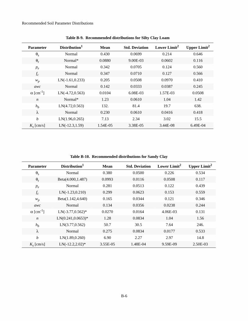
Recommended Soil Parameter Distributions
Table B-9. Recommended distributions for Silty Clay Loam
Parameter Distribution1 Mean Std. Deviation Lower Limit2 Upper Limit2
θs Normal 0.430 0.0699 0.214 0.646
θr Normal* 0.0880 9.00E-03 0.0602 0.116
pe Normal 0.342 0.0705 0.124 0.560
fc Normal 0.347 0.0710 0.127 0.566
wp LN(-1.61,0.233) 0.205 0.0508 0.0970 0.410
awc Normal 0.142 0.0333 0.0387 0.245
α [cm-1] LN(-4.72,0.563) 0.0104 6.08E-03 1.57E-03 0.0508
n Normal* 1.23 0.0610 1.04 1.42
hb LN(4.72,0.563) 132. 81.4 19.7 638.
λ Normal 0.230 0.0610 0.0416 0.418
b LN(1.96,0.265) 7.13 2.34 3.02 15.5
Ks [cm/s] LN(-12.3,1.59) 1.54E-05 3.38E-05 3.44E-08 6.49E-04
Table B-10. Recommended distributions for Sandy Clay
Std. Deviation Lower Limit2 Upper Limit2
0.0500 0.226 0.534
0.0116 0.0508 0.117
0.0513 0.122 0.439
0.0623 0.153 0.559
0.0344 0.121 0.346
0.0356 0.0238 0.244
0.0164 4.06E-03 0.131
0.0834 1.04 1.56
30.5 7.64 246.
0.0834 0.0177 0.533
2.27 2.97 14.8
1.48E-04 9.59E-09 2.50E-03
Parameter Distribution1 Mean
θs Normal 0.380
θr Beta(4.000,1.487) 0.0993
pe Normal 0.281
fc LN(-1.23,0.210) 0.299
wp Beta(1.142,4.640) 0.165
awc Normal 0.134
α [cm-1] LN(-3.77,0.562)* 0.0270
n LN(0.241,0.0653)* 1.28
hb LN(3.77,0.562) 50.7
λ Normal 0.275
b LN(1.89,0.260) 6.90
Ks [cm/s] LN(-12.2,2.02)* 3.55E-05
B-6

Recommended Soil Parameter Distributions
Table B-11. Recommended distributions for Silty Clay
Parameter Distribution1 Mean Std. Deviation Lower Limit2 Upper Limit2
θs Normal 0.360 0.0698 0.144 0.576
θr Normal* 0.0706 0.0228 1.47E-04 0.141
pe Normal 0.289 0.0735 0.0623 0.517
fc Normal 0.334 0.0678 0.124 0.543
wp LN(-1.49,0.220) 0.230 0.0512 0.114 0.444
awc Normal 0.103 0.0303 9.63E-03 0.197
α [cm-1] LN(-5.66,0.584)* 4.13E-03 2.60E-03 5.73E-04 0.0211
n LN(0.145,0.0430) 1.16 0.0499 1.01 1.32
hb LN(5.66,0.584) 340. 216. 47.3 1743.
λ Beta(2.591,3.268) 0.157 0.0499 0.0404 0.304
b LN(2.29,0.259) 10.2 2.96 4.43 22.0
Ks [cm/s] LN(-13.9,1.31)* 2.19E-06 4.08E-06 1.64E-08 5.37E-05
Table B-12. Recommended distributions for Clay
Parameter Distribution1 Mean Std. Deviation Lower Limit2 Upper Limit2
θs Normal 0.380 0.0900 0.102 0.658
θr Beta(1.501,1.580) 0.0685 0.0344 8.36E-04 0.140
pe Normal 0.311 0.0963 0.0138 0.609
fc Normal 0.340 0.0893 0.0638 0.615
wp Beta(2.751,4.921) 0.263 0.0770 0.0939 0.567
awc LN(-2.66,0.429) 0.0761 0.0299 0.0186 0.263
α [cm-1] LN(-5.54,0.893) 6.18E-03 7.59E-03 2.50E-04 0.0621
n Beta(0.8857,2.400) 1.13 0.0697 1.04 1.36
hb Beta(0.8002,1.546) 353. 257. 14.1 1007
λ Beta(0.8854,2.399) 0.127 0.0697 0.0397 0.365
b Beta(1.751,11.61) 14.1 6.24 4.93 75.0
Ks [cm/s] LN(-12.36,2.269) 3.65E-05 1.08E-04 3.87E-09 4.76E-03
1. LN(,) = Lognormal(γ,ζ); see Section B.2. Beta(,) =Beta(q,r); see Section B.3.
2. Lower Limit and Upper Limit are 0.001 and 0.999 quantiles for Normal and Lognormal distributions.
* Indicates that the recommended distribution is the same type as used by Carsel and Parrish (1988). This applies to the parameters θr, α, n, and Ks only.
B-7

Recommended Soil Parameter Distributions
B.5 References
Ang, A. H-S. and W. H. Tang, Probability Concepts in Engineering Planning and Design, Volume 1, Basic Princi-ples, John Wiley & Sons, New York, 409 pp., 1975.
Carsel, R. F., and R. S. Parrish, “Developing joint probabil-ity distributions of soil water retention characteristics,” Water Resources Research, 24(5):755-770, 1988.
Meyer, P.D., M.L. Rockhold, and G.W. Gee, “Uncertainty Analyses of Infiltration and Subsurface Flow and Transport for SDMP Sites,” NUREG/CR-6565, U.S. Nuclear Regula-tory Commission, Washington, DC, 1997.
B-8

Appendix C: Soil Parameter Correlation Coefficients
The correlation coefficient is a measure of the strength of a linear relationship between two random variables (i.e., soil parameters), X and Y. Sample correlation coefficients were calculated as follows [e.g., Ang and Tang (1975)].
(C-1)
where
= sample correlation coefficient
xi, yi = sample values for parameters X and Y
= sample mean values calculated as
(C-2)
sx, sy = sample standard deviations calculated as
(C-3)
N = the number of sample values
Correlations between parameters were induced by applying the correlations between θr, α, n, and Ks given in Carsel and Parrish (1988). The rank correlation method of Iman and Conover (1982) as embodied in the Latin hypercube sam-pling code of Iman and Shortencarier (1984) was used. Note that the correlations given in the tables below do not neces-sarily appear to be the same as those of Carsel and Parrish (1988) since their correlations were calculated after the parameters were transformed to normal distributions. The correlations given below were calculated on the untrans-formed parameters. Definitions of parameters in the tables can be found in Appendix D.
This appendix was originally presented in NUREG/CR-6565 (Meyer et al., 1997).
ρ̂ 1N 1–-------------
xiyi
i 1=
N
∑ Nxy–
sxsy---------------------------------=
ρ̂
x y,
x1N---- xi
i 1=
N
∑=
sx2 1
N 1–------------- xi x–( )
2
i 1=
N
∑=
Table C-1. Correlation coefficients for Sand
θs θr pe fc wp awc α n hb λ b Ks
θs 1 -0.01 0.99 0.15 -0.01 0.38 0.00 0.00 -0.02 0.00 -0.29 0.00
θr 1 -0.18 0.94 1 0.59 0.12 -0.84 -0.12 -0.84 0.91 -0.50
pe 1 -0.02 -0.18 0.27 -0.02 0.15 0.01 0.15 -0.44 0.08
fc 1 0.94 0.82 -0.11 -0.91 0.11 -0.91 0.89 -0.67
wp 1 0.59 0.12 -0.84 -0.12 -0.84 0.91 -0.50
awc 1 -0.49 -0.79 0.49 -0.79 0.59 -0.78
α 1 0.29 -0.97 0.29 -0.09 0.73
n 1 -0.28 1 -0.88 0.84
hb 1 -0.28 0.09 -0.68
λ 1 -0.88 0.84
b 1 -0.65
Ks 1
C-1

Soil Parameter Correlation Coefficients
Table C-2. Correlation coefficients for Loamy Sand
θs θr pe fc wp awc α n hb λ b Ks
θs 1 -0.01 0.99 0.27 0.00 0.49 0.00 0.01 -0.03 0.01 -0.50 0.01
θr 1 -0.16 0.85 1 0.34 -0.29 -0.58 0.16 -0.58 0.71 -0.34
pe 1 0.13 -0.16 0.42 0.05 0.10 -0.05 0.10 -0.60 0.07
fc 1 0.85 0.79 -0.53 -0.76 0.33 -0.76 0.57 -0.58
wp 1 0.35 -0.30 -0.58 0.17 -0.58 0.72 -0.35
awc 1 -0.60 -0.68 0.39 -0.68 0.19 -0.63
α 1 0.38 -0.57 0.38 -0.29 0.88
n 1 -0.22 1 -0.64 0.65
hb 1 -0.22 0.17 -0.38
λ 1 -0.64 0.65
b 1 -0.41
Ks 1
Table C-3. Correlation coefficients for Sandy Loam
θs θr pe fc wp awc α n hb λ b Ks
θs 1 0.00 0.98 0.38 0.03 0.54 0.01 0.00 0.01 0.00 -0.44 0.01
θr 1 -0.19 0.72 1 0.34 0.14 -0.79 -0.17 -0.79 0.77 -0.22
pe 1 0.24 -0.16 0.46 -0.02 0.15 0.04 0.15 -0.57 0.05
fc 1 0.78 0.90 -0.35 -0.85 0.35 -0.85 0.51 -0.51
wp 1 0.42 0.08 -0.82 -0.10 -0.82 0.77 -0.25
awc 1 -0.56 -0.65 0.57 -0.65 0.20 -0.56
α 1 0.36 -0.77 0.36 -0.11 0.82
n 1 -0.28 1 -0.78 0.60
hb 1 -0.28 0.05 -0.51
λ 1 -0.78 0.60
b 1 -0.33
Ks 1
C-2

Soil Parameter Correlation Coefficients
Table C-4. Correlation coefficients for Sandy Clay Loam
θs θr pe fc wp awc α n hb λ b Ks
θs 1 0.00 1 0.48 0.21 0.58 -0.01 0.00 -0.02 0.00 -0.43 -0.01
θr 1 -0.09 -0.02 0.23 -0.16 0.37 -0.11 -0.36 -0.11 0.21 0.16
pe 1 0.48 0.19 0.59 -0.04 0.01 0.01 0.01 -0.45 -0.03
fc 1 0.88 0.97 -0.67 -0.81 0.66 -0.81 0.42 -0.50
wp 1 0.73 -0.51 -0.81 0.68 -0.81 0.65 -0.33
awc 1 -0.69 -0.73 0.58 -0.73 0.24 -0.54
α 1 0.77 -0.70 0.77 -0.49 0.82
n 1 -0.65 1 -0.76 0.71
hb 1 -0.65 0.57 -0.39
λ 1 -0.76 0.71
b 1 -0.38
Ks 1
Table C-5. Correlation coefficients for Loam
θs θr pe fc wp awc α n hb λ b Ks
θs 1 0.00 0.99 0.55 0.18 0.63 0.03 0.00 0.04 0.00 -0.46 0.03
θr 1 -0.13 0.29 0.79 -0.03 -0.04 -0.70 0.07 -0.70 0.67 0.14
pe 1 0.50 0.08 0.63 0.03 0.09 0.03 0.09 -0.54 0.01
fc 1 0.75 0.93 -0.63 -0.71 0.70 -0.71 0.28 -0.41
wp 1 0.47 -0.42 -0.87 0.56 -0.87 0.69 -0.16
awc 1 -0.62 -0.49 0.63 -0.49 0.00 -0.46
α 1 0.60 -0.73 0.60 -0.37 0.82
n 1 -0.55 1 -0.79 0.41
hb 1 -0.55 0.39 -0.42
λ 1 -0.79 0.41
b 1 -0.21
Ks 1
C-3

Soil Parameter Correlation Coefficients
Table C-6. Correlation coefficients for Silt Loam
θs θr pe fc wp awc α n hb λ b Ks
θs 1 -0.01 0.98 0.48 0.20 0.70 -0.02 -0.01 -0.02 -0.01 -0.20 -0.02
θr 1 -0.18 0.50 0.66 0.18 -0.29 -0.59 0.27 -0.59 0.63 -0.25
pe 1 0.39 0.08 0.66 0.03 0.10 -0.06 0.10 -0.31 0.03
fc 1 0.91 0.87 -0.72 -0.80 0.73 -0.80 0.63 -0.45
wp 1 0.58 -0.63 -0.89 0.73 -0.89 0.86 -0.36
awc 1 -0.65 -0.50 0.54 -0.50 0.20 -0.44
α 1 0.74 -0.75 0.74 -0.56 0.80
n 1 -0.69 1 -0.88 0.48
hb 1 -0.69 0.68 -0.39
λ 1 -0.88 0.48
b 1 -0.31
Ks 1
Table C-7. Correlation coefficients for Silt
θs θr pe fc wp awc α n hb λ b Ks
θs 1 -0.02 1 0.90 0.52 0.97 0.00 0.00 0.03 0.00 -0.39 0.02
θr 1 -0.10 0.25 0.57 -0.02 -0.19 -0.60 0.04 -0.60 0.70 -0.21
pe 1 0.88 0.48 0.96 0.01 0.05 0.03 0.05 -0.44 0.04
fc 1 0.81 0.92 -0.35 -0.37 0.16 -0.37 -0.03 -0.30
wp 1 0.51 -0.60 -0.72 0.48 -0.72 0.44 -0.45
awc 1 -0.10 -0.06 -0.09 -0.06 -0.35 -0.14
α 1 0.55 -0.49 0.55 -0.41 0.89
n 1 -0.20 1 -0.84 0.44
hb 1 -0.20 0.13 -0.29
λ 1 -0.84 0.44
b 1 -0.34
Ks 1
C-4

Soil Parameter Correlation Coefficients
Table C-8. Correlation coefficients for Clay Loam
θs θr pe fc wp awc α n hb λ b Ks
θs 1 0.00 0.99 0.65 0.38 0.76 -0.02 0.00 -0.04 0.00 -0.40 0.01
θr 1 -0.11 -0.50 -0.46 -0.43 0.73 0.58 -0.74 0.58 -0.35 0.51
pe 1 0.69 0.43 0.80 -0.10 -0.06 0.04 -0.06 -0.36 -0.04
fc 1 0.89 0.90 -0.60 -0.71 0.55 -0.71 0.23 -0.42
wp 1 0.60 -0.55 -0.84 0.75 -0.84 0.57 -0.33
awc 1 -0.52 -0.45 0.26 -0.45 -0.13 -0.42
α 1 0.79 -0.62 0.79 -0.42 0.89
n 1 -0.80 1 -0.73 0.58
hb 1 -0.80 0.70 -0.36
λ 1 -0.73 0.58
b 1 -0.26
Ks 1
Table C-9. Correlation coefficients for Silty Clay Loam
θs θr pe fc wp awc α n hb λ b Ks
θs 1 0.00 0.99 0.73 0.46 0.85 -0.01 0.00 0.00 0.00 -0.19 -0.03
θr 1 -0.13 -0.42 -0.46 -0.21 0.72 0.55 -0.71 0.55 -0.37 0.47
pe 1 0.77 0.51 0.87 -0.10 -0.07 0.10 -0.07 -0.15 -0.09
fc 1 0.90 0.75 -0.62 -0.65 0.58 -0.65 0.35 -0.45
wp 1 0.40 -0.68 -0.84 0.79 -0.84 0.69 -0.42
awc 1 -0.29 -0.11 0.02 -0.11 -0.30 -0.32
α 1 0.86 -0.75 0.86 -0.57 0.83
n 1 -0.84 1 -0.82 0.60
hb 1 -0.84 0.80 -0.41
λ 1 -0.82 0.60
b 1 -0.32
Ks 1
C-5

Soil Parameter Correlation Coefficients
Table C-10. Correlation coefficients for Sandy Clay
θs θr pe fc wp awc α n hb λ b Ks
θs 1 0.00 0.97 0.58 0.35 0.68 0.02 0.00 0.01 0.00 -0.23 0.05
θr 1 -0.23 -0.70 -0.82 -0.42 0.75 0.88 -0.92 0.88 -0.78 0.28
pe 1 0.72 0.53 0.75 -0.15 -0.20 0.22 -0.20 -0.05 -0.02
fc 1 0.89 0.89 -0.70 -0.78 0.68 -0.78 0.44 -0.33
wp 1 0.58 -0.67 -0.85 0.87 -0.85 0.74 -0.24
awc 1 -0.58 -0.55 0.35 -0.55 0.05 -0.35
α 1 0.87 -0.74 0.87 -0.59 0.58
n 1 -0.86 1 -0.79 0.44
hb 1 -0.86 0.83 -0.26
λ 1 -0.79 0.44
b 1 -0.23
Ks 1
Table C-11. Correlation coefficients for Silty Clay
θs θr pe fc wp awc α n hb λ b Ks
θs 1 0.00 0.95 0.94 0.74 0.84 -0.01 -0.01 -0.01 -0.01 -0.31 0.02
θr 1 -0.31 -0.29 -0.49 0.19 0.89 0.79 -0.88 0.79 -0.46 0.64
pe 1 0.98 0.86 0.74 -0.28 -0.25 0.26 -0.25 -0.15 -0.18
fc 1 0.91 0.70 -0.32 -0.33 0.24 -0.33 -0.07 -0.24
wp 1 0.34 -0.50 -0.64 0.52 -0.64 0.32 -0.34
awc 1 0.14 0.33 -0.36 0.33 -0.70 0.03
α 1 0.84 -0.72 0.84 -0.47 0.86
n 1 -0.78 1 -0.77 0.64
hb 1 -0.78 0.63 -0.44
λ 1 -0.77 0.64
b 1 -0.31
Ks 1
C-6
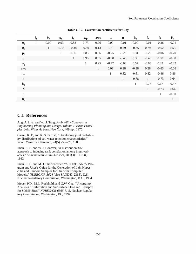
Soil Parameter Correlation Coefficients
C.1 References
Ang, A. H-S. and W. H. Tang, Probability Concepts in Engineering Planning and Design, Volume 1, Basic Princi-ples, John Wiley & Sons, New York, 409 pp., 1975.
Carsel, R. F., and R. S. Parrish, “Developing joint probabil-ity distributions of soil water retention characteristics,” Water Resources Research, 24(5):755-770, 1988.
Iman, R. L. and W. J. Conover, “A distribution-free approach to inducing rank correlation among input vari-ables,” Communications in Statistics, B11(3):311-334, 1982.
Iman, R. L. and M. J. Shortencarier, “A FORTRAN 77 Pro-gram and User’s Guide for the Generation of Lain Hyper-cube and Random Samples for Use with Computer Models,” NUREG/CR-3624 (also SAND83-2365), U.S. Nuclear Regulatory Commission, Washington, D.C., 1984.
Meyer, P.D., M.L. Rockhold, and G.W. Gee, “Uncertainty Analyses of Infiltration and Subsurface Flow and Transport for SDMP Sites,” NUREG/CR-6565, U.S. Nuclear Regula-tory Commission, Washington, DC, 1997.
Table C-12. Correlation coefficients for Clay
θs θr pe fc wp awc α n hb λ b Ks
θs 1 0.00 0.93 0.88 0.73 0.76 0.00 -0.01 0.00 -0.01 -0.26 -0.01
θr 1 -0.36 -0.38 -0.50 0.13 0.70 0.79 -0.85 0.79 -0.52 0.53
pe 1 0.96 0.85 0.66 -0.25 -0.29 0.31 -0.29 -0.06 -0.20
fc 1 0.95 0.55 -0.38 -0.45 0.36 -0.45 0.08 -0.30
wp 1 0.25 -0.47 -0.63 0.57 -0.63 0.33 -0.32
awc 1 0.09 0.28 -0.38 0.28 -0.63 -0.06
α 1 0.82 -0.61 0.82 -0.46 0.86
n 1 -0.78 1 -0.73 0.64
hb 1 -0.78 0.67 -0.37
λ 1 -0.73 0.64
b 1 -0.30
Ks 1
C-7


Appendix D: Summary of Water Retention and Conductivity Models
This appendix defines the parameters appearing in the tables of Appendices B and C. The information in this appendix was taken from NUREG/CR-6565 (Meyer et al., 1997).
Richards equation (Richards, 1931) forms the basis for most process-based descriptions of water movement in the unsat-urated zone. Richards equation can be expressed as
(D-1)
where
θ = volumetric water content, or volume of water per unit bulk volume of soil,
h = soil water tension, h ≥ 0
z = depth, measured positive downward from the soil surface,
t = time,
K(h) = hydraulic conductivity, and
u = a source or sink term used to account for water uptake by plant roots.
To solve Richards equation, constitutive functions relating the unsaturated hydraulic conductivity and the water content to the pressure head are needed. The most commonly used relationships are those of van Genuchten (1980), Brooks and Corey (1964), and Campbell (1974), although other expres-sions are available (Mualem, 1992; Rossi and Nimmo, 1994; Fayer and Simmons, 1995).
D.1 Van Genuchten Model
The van Genuchten water retention relationship is
(D-2)
where
Se = effective saturation = , 0 ≤Se ≤ 1
α = curve fitting parameter related to air entry pressure
n, m = curve fitting parameters related to pore size distribution; the relationship, m=1-1/n, is often assumed
θr = residual water content
θs = saturated water content
The van Genuchten hydraulic conductivity relationship, based on the hydraulic conductivity model of Mualem (1976) is
. (D-3)
or
(D-4)
where
Ks = saturated hydraulic conductivity
D.2 Brooks-Corey ModelThe Brooks-Corey water retention relationship is
for h ≥ hb (D-5)
otherwise. (D-6)
When combined with the relative permeability model of Burdine (1953), Brooks and Corey derived the following hydraulic conductivity relationship.
(D-7)
or
for h ≥ hb (D-8)
and otherwise. (D-9)
where
hb = curve fitting parameter related to air entry pressure
λ = curve fitting parameter related to pore size dis-tribution.
Carsel and Parrish (1988) used the following equivalence between the Brooks-Corey and van Genuchten parameters:
hb = α-1 and λ = n - 1.
D.3 Campbell ModelCampbell (1974) adopted a water retention relationship sim-ilar to Brooks and Corey’s, but with θr = 0.
for h ≥ hb (D-10)
otherwise. (D-11)
Note that because θr = 0, b ≠ 1/λ. Campbell (1974) derived a corresponding hydraulic conductivity relationship.
t∂∂θ
z∂∂ K– h( )
z∂∂h
K h( )– u+=
Se h( ) 1 αh( )n+[ ] m–=
θ θr–
θs θr–----------------
K Se( ) Ks Se 1 1 Se1 m⁄–( )
m–[ ]
2=
K h( ) Ks1 αh( )n 1– 1 αh( )n+[ ]
m––{ }
2
1 αh( )n+[ ]0.5m
-------------------------------------------------------------------------=
Se h( )hb
h-----
λ
=
Se h( ) 1=
K Se( ) Ks Se( )3 2 λ⁄+=
K h( ) Ks
hb
h-----
2 3λ+
=
K h( ) Ks=
θθs----
hb
h-----
1 b⁄
=
θθs---- 1=
D-1

Summary of Water Retention and Conductivity Models
(D-12)
or
for h ≥ hb (D-13)
and otherwise. (D-14)
where
b = curve fitting parameter related to pore size distribution.
Note that all of these single-valued relationships (Equations D-2 through D-14) assume that hysteresis is not important.
D.3.1 Calculation of Campbell’s b Parameter
An expression for b in terms of θs, θr, and λ is derived by assuming that the Brooks-Corey model (Equation D-7) and the Campbell model (Equation D-12) predict the same hydraulic conductivity for a given value of water content. In this case, the water content used is that corresponding to an effective saturation of 0.5. Assuming Se = 0.5 and using the definition of effective saturation given above, it follows that
(D-15)
Substituting this expression in Equation D-12 and equating this with Equation D-7 leads to
(D-16)
Equation D-16 can be solved for b,
(D-17)
D.4 Additional Parameters
Several additional soil hydraulic parameters may be required by dose assessment codes. These parameters and the methods by which they were calculated are discussed here.
• Effective porosity, pe = θs - θr• Field capacity, fc = θ(K = 10-8 cm/s)
Field capacity is generally interpreted as the water con-tent at which drainage from a field soil becomes negligi-ble (see the discussion by Hillel, 1980). Field capacity is often calculated as the water content at a specified ten-sion, usually taken to be 340 cm (1/3 bar). Hillel (1980) argues, however, that the field capacity should be based on the drainage rate considered negligible (which is a
K θ( ) Ksθθs----
2b 3+=
K h( ) Ks
hb
h-----
2 3 b⁄+
=
K h( ) Ks=
θθs----
0.5 θs θr–( ) θr+
θs---------------------------------------- 0.5 1 θr θs⁄+( )= =
0.5 1 θr θs⁄+( )( )3 2b+ 0.53 2 λ⁄+=
b 0.5 0.5( ) 3 2 λ⁄+( )ln0.5 1 θr θs⁄+( )[ ]ln
---------------------------------------------- 3–
=
D-2
function of the intended application). Field capacity was calculated here as the water content at which the unsat-urated hydraulic conductivity equals 10-8 cm/s using the van Genuchten model (10-8 cm/s ≅ 3 mm/yr).The value of 10-8 cm/s was chosen because it represents a water flux at which contaminant transport is likely to be insig-nificant. This value also results in somewhat larger field capacity values and a more realistic available water capacity for very coarse textured soils than using the water content at 1/3 bar soil pressure. See Meyer and Gee (1999) for a more detailed discussion of field capac-ity.
• Wilting point, wp = θ(h = 15,300 cm)Wilting point is the minimum water content (or maxi-mum tension) at which plants can extract water from the soil. Wilting point was calculated as the water content at a tension of 15,300 cm (15 bars).
• Available water capacity, awc = fc - wpAvailable water capacity represents the amount of water available for plant uptake.
D.5 ReferencesBrooks, R. H., and A. T. Corey, “Hydraulic Properties of Porous Media,” Hydrology Paper 3, Colorado State Univ., Ft. Collins, CO, 1964.
Burdine, N. T. “Relative permeability calculations from pore-size distribution data.” Petr. Trans., Am. Inst. Mining Metall. Eng., 198:71-77, 1953.
Campbell, G. S., “A simple method for determining unsatur-ated conductivity from moisture retention data,” Soil Sci., 117:311-314, 1974.
Fayer, M. J., and C. S. Simmons, “Modified soil water retention functions for all matric suctions,” Water Resources Research, 31:1233-1238, 1995.
Meyer, P.D., M.L. Rockhold, and G.W. Gee, “Uncertainty Analyses of Infiltration and Subsurface Flow and Transport for SDMP Sites,” NUREG/CR-6565, U.S. Nuclear Regula-tory Commission, Washington, DC, 1997.
Meyer, P. D. and G. W. Gee, “Flux-based estimation of field capacity,” Journal of Geotechnical and Geoenvironmental Engineering, 125(7):595-599, 1999.
Mualem, Y., “A new model for predicting the hydraulic con-ductivity of unsaturated porous media,” Water Resources Research, 12(3):513-522, 1976.
Mualem, Y., “Modeling the Hydraulic Conductivity of Unsaturated Porous Media,” in Indirect Methods for Esti-mating the Hydraulic Properties of Unsaturated Soils, M. Th. van Genuchten, F. J. Leij, and L. J. Lund (eds.), Univer-sity of California, Riverside, CA, pp. 15-36, 1992.

Summary of Water Retention and Conductivity Models
Rossi, C. and J. R. Nimmo, “Modeling of soil water reten-tion from saturation to oven dryness,” Water Resources Research, 30(3):701-708, 1994.
van Genuchten, M. Th., “A closed-form equation for predict-ing the hydraulic conductivity of unsaturated soils,” Soil Sci. Soc. Am. J., 44:892-898, 1980.
D-3