Embed Size (px)
Citation preview

HYDRODYNAMIC CHARACTERISTIC STUDY OF A THREE
PHASE CO-CURRENT TRICKLE-BED REACTOR: CFD ANALYSIS
A thesis submitted in partial fulfillment of the requirements for the degree of Bachelor of Technology
In
Chemical Engineering
By
Bidhu Bhusan Meher Roll No. 107CH032
Under the guidance of
Dr. H. M. Jena
DEPARTMENT OF CHEMICAL ENGINEERING NATIONAL INSTITUTE OF TECHNOLOGY, ROURKELA
ORISSA -769 008, INDIA 2011

i
CERTIFICATE
This is to certify that the thesis entitled “Hydrodynamic Characteristic Study of
a Three Phase Co-current Trickle-Bed Reactor: CFD analysis” being submitted
by Bidhu Bhusan Meher (107CH032) as an academic project in the Department of
Chemical Engineering, National Institute of Technology, Rourkela is a record of bonafide
work carried out by him under my guidance and supervision.
Place: Dr. H. M. Jena
Date: Department of Chemical Engineering
National Institute of Technology
Rourkela - 769008
INDIA

ii
ACKNOWLEDGEMENT
I wish to express my sincere thanks and gratitude to Prof. Dr. H. M. Jena (Project Guide) for
suggesting me the topic and providing me the guidance, motivation and constructive criticism
throughout the course of the project.
I also express my sincere gratitude to Prof. Dr. K. C. Biswal (HOD) and Prof. Dr. R. K. Singh
(Project Coordinator), of Department of Chemical Engineering, National Institute of
Technology, Rourkela, for their valuable guidance and timely suggestions during the entire
duration of my project work, without which this work would not have been possible. I am
also grateful to Department, Chemical Engineering for providing me the necessary
opportunities for the completion of my project.
Bidhu Bhusan Meher
107CH032

iii
ABSTRACT
Trickle-bed has been extensively used in chemical process industries mainly in petrochemical
and refinery process since it provide flexibility and simplicity of operation as well as high
throughputs. The basic parameter for design, scale-up and operations of a trickle bed reactor
are the pressure gradient and liquid saturation. Knowledge of these hydrodynamics
parameters and prevailing flow regime is essential for design and performance evaluation of
the reactor. But hydrodynamics of trickle bed reactor involve complex interaction of gas and
liquid phase with packed solid which is very difficult to understand. Many computational
models have been developed and extensive CFD study of hydrodynamics parameters has
been done is last few decades to understand the behaviour of trickle bed reactor.
In the present work an attempt has been made to study the hydrodynamics of a co-current
gas-liquid-solid trickle bed reactor using FLUENT 6.3.26. CFD simulations has been done
using Eulerian-Eulerian approach for a trickle bed system with column of height 1 m and
diameter 0.194 m containing glass beads of diameter 6mm as solid packing. GAMBIT 2.3.16
has been used to generate a 2D coarse grid. The phase holdup and pressure drop behaviours
have been studied and their axial and radial distributions have been illustrated. The results
show that liquid holdup increases with increase in liquid velocity and decrease with increase
in gas velocity. The trend is reverse for gas holdup i.e. it increases with increase in gas
velocity and decrease with increase in liquid velocity. Pressure drop increases with increase
in both gas and liquid velocity. Quantification of this behaviour has been done. The results
have been compared with previous literature data available and found to agree well.
Keywords: Hydrodynamics, Trickle-bed reactor, Liquid holdup, Pressure Drop, CFD
iv
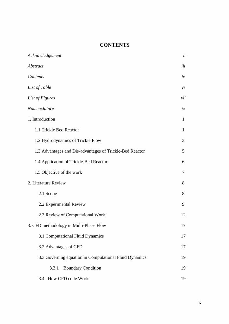
CONTENTS
Acknowledgement ii
Abstract iii
Contents iv
List of Table vi
List of Figures
Nomenclature
vii
ix
1. Introduction
1.1 Trickle Bed Reactor
1.2 Hydrodynamics of Trickle Flow
1.3 Advantages and Dis-advantages of Trickle-Bed Reactor
1.4 Application of Trickle-Bed Reactor
1.5 Objective of the work
1
1
3
5
6
7
2. Literature Review
2.1 Scope
2.2 Experimental Review
2.3 Review of Computational Work
8
8
9
12
3. CFD methodology in Multi-Phase Flow
3.1 Computational Fluid Dynamics
3.2 Advantages of CFD
3.3 Governing equation in Computational Fluid Dynamics
3.3.1 Boundary Condition
3.4 How CFD code Works
17
17
17
19
19
19

v
3.4.1 pre-processing
3.4.2 solver
3.4.3 Post-Processing
3.5 CFD approach in Multiphase Flow
3.5.1 The Euler-Lagrange Approach
3.5.2 The Euler-Euler Approach
3.6 Some multiphase system
3.7 Choosing a multiphase model
19
20
22
23
23
23
25
25
4. CFD simulation of three phase co-current trickle-bed
4.1 Computational Flow Model
4.1.1 Equation Reformulation
4.1.2 Turbulence Modelling
4.2 Problem Description for simulation
4.3 Geometry and Mesh
4.4 Assumptions
4.5 Solution
26
26
26
27
28
28
29
29
5. Results and discussion
5.1 Phase Dynamics
5.1.1 Liquid Holdup
5.1.2 Gas Holdup
5.1.3 Pressure Drop
5.2 Comparison with Literature Data
31
32
34
37
40
42
6. Conclusions 44
References 46

vi
LIST OF TABLES
Table no Caption Page no
Table 2.1 Various Models Proposed for Trickle-bed Reactor 15
Table 4.1 The model constants used for turbulence modeling 27
Table 4.2 Properties of Air and Water 28
Table 4.3 Models used for considering interactions among phases. 30
Table 4.4 Solution Control Parameters 30
Table 5.1 Experimental set-up parameters of various work in literature. 42

vii
LIST OF FIGURES
Figure no Caption Page no
Figure 1.1 Co-current down flow regime in a trickle bed 4
Figure 1.2 Gas and liquid flow pattern in a Trickle-Flow 4
Figure 3.1 Flowchart showing the general procedure for the simulation
using Fluent
22
Figure 4.1 The unstructured grid developed for the simulation 28
Figure 5.1 Contour of volume fraction of air for air velocity 0.14 m/s and
liquid velocity 0.009 m/s.
31
Figure 5.2 Contour of volume fraction of liquid, gas and solid phase at
gas velocity of 0.11m/s and liquid velocity of 0.005m/s.
32
Figure 5.3 Velocity vector of water and air 33
Figure 5.4 Radial variation of velocity of liquid at a height of Z=0.5 m at
gas velocity of 0.2m/s
34
Figure 5.5 liquid holdup for different liquid velocity 34
Figure 5.6 liquid holdup for different gas velocity 34
Figure 5.7 Liquid Holdup variation with Height of the column at liquid
velocity of 0.003m/s and 0.011m/s.(gas velocity= 0.2m/s)
35
Figure 5.8(a) Radial Averaged Liquid Holdup variation along the diameter
of the column at different height at gas velocity of 0.11m/s
and liquid velocity 0.009 m/s
36
Figure 5.8(b) Radial Averaged Liquid Holdup variation along the diameter
of the column at different height at gas velocity of 0.20m/s
and liquid velocity 0.009 m/s
36
Figure 5.9 Gas holdup for different liquid velocity 37

viii
Figure 5.10 Gas holdup for different gas velocity 37
Figure 5.10 Gas Holdup variation with Height of the column at liquid
velocity of 0.003m/s and 0.011m/s. (gas velocity= 0.2m/s)
38
Figure 5.11(a) Gas Holdup variation along the diameter of the column at
different height at gas velocity of 0.20m/s and liquid velocity
0.003 m/s
39
Figure 5.11(a) Gas Holdup variation along the diameter of the column at
different height at gas velocity of 0.20m/s and liquid velocity
0.009 m/s
39
Figure 5.12 Pressure drop per unit length with different liquid and gas
flow velocity.
40
Figure 5.13 Pressure drop along axial length of the bed. 40
Figure 5.14 Radial-Averaged Pressure drop along the diameter of the
column at different height at gas velocity of 0.2m/s and liquid
velocity 0.003 m/s
41
Figure 5.15 Pressure drop Comparison with previous work 42
Figure 5.16 comparison of liquid holdup of along the diameter of the
column at a height 0.879 Z at gas velocity of 0.11m/s with
previous work
43

ix
NOMENCLATURE
g= Acceleration due to gravity, m/s2
ρk = Density of phase k= g (gas), l (liquid), kg/m3
ε= Dissipation rate of turbulent kinetic energy, m2s
-3
μeff= Effective viscosity, kg/m-s
Mi,g= Interphase force term for gas phase
Mi,l= Interphase force term for liquid phase
P= Pressure, Pa
t= Time, s
k= Turbulent kinetic energy, J
Uk= Velocity of phase k= g (gas), l (liquid), s (solid), m/s
αk= Volume fraction of phase k= g (gas), l (liquid), such that αL+αG=1
D = Diameter of the column, m
x = Radial Position in the column, m
Z= Height of the column, m
1
CHAPTER 1
INTRODUCTION
1.1 Trickle Bed Reactor:
Trickle bed reactor is a packed bed of stationary particle that are subjected to co-current gas
and liquid flow at relatively low fluid superficial velocities. It is considered to be the simplest
reactor type for performing catalytic reactions. TBRs find widespread use in petroleum
refining, chemical and process industries, pollution treatment and biochemical industries.
Design and scale up of TBRs continues to be a major challenge for chemical engineers. A
rigorous and fundamentally exhaustive mathematical description of trickle flow dynamics has
not been achieved. The design and scale-up of trickle bed reactors depend on key
hydrodynamic variables such as liquid volume fraction (liquid saturation), particle scale
wetting and overall gas–liquid distribution. Some of the important chemical engineering
aspects for design of Trickle-bed reactor are: (Sie and Krishna, 1998)
1. Pressure Drop
2. Liquid and Gas Holdups
3. Catalyst Contacting
4. Axial and Radial Dispersion of liquid and gas
5. Mass Transfer
6. Heat Transfer
7. Thermal stability
These variables are difficult to determine experimentally and interactions between these are
as yet poorly understood. Even though numerous experimental studies have been reported in
measurement of these variables, predicting them from first principle hydrodynamic
2
simulations is difficult as yet and no coherent and conclusive methodology for doing so has
yet been espoused. In order to explain the hydrodynamics of trickle bed reactor many models
and approaches has been proposed by the authors.
In trickle bed reactor Hydrodynamics is quantified in terms of hydrodynamics parameter like
pressure drop, liquid holdup, gas holdup, liquid mal-distribution which are related in some
way to the gas-liquid-solid contacting effectiveness and operational efficiency of the reactor
column. A phenomenon that greatly complicates the mathematical description of trickle bed
reactor is that these hydrodynamic variables are path variable, which depend on the history of
the operation. This phenomenon manifests itself in the form of hysteresis loops or multiple
hydrodynamics state.
Factors that affect the performance of a trickle bed reactor are:
Porosity: increase in porosity decreases liquid and gas holdup, pressure drop, wetting
deficiency and mal-distribution factor, however it increases gas-liquid mass transfer
rate, liquid solid mass transfer rate and axial dispersion of fluid.(Kundu et al, 2001)
Particle size: increase in particle size decreases liquid and gas holdup, pressure drop,
mass transfer rate and wetting efficiency but increases axial dispersion and mal-
distribution factor. .(Kundu et al, 2001)
Liquid density: increase in liquid density increases pressure drop and give poor
performance in mass transfer and wetting efficiency.
Liquid viscosity: it promotes holdup, pressure drop, gas-liquid mass transfer and
wetting efficiency but decrease axial dispersion of liquid.
Surface tension: increase in surface tension of liquid increases pressure drop but
decreases gas-liquid mass transfer and wetting efficiency.( Saroha et al, 2008)
Liquid superficial velocity: this promotes liquid holdup, pressure drop, mass-transfer,
wetting efficiency and axial dispersion and decreases mal-distribution of liquid.

3
Gas superficial velocity: this decreases the liquid holdup and mal-distribution but
increases pressure drop, mass transfer and wetting efficiency.
Gas viscosity: increase in gas viscosity promotes holdup, pressure drop, liquid-gas
mass transfer rate.( Wang et al, 1997)
Pressure (gas density) : increase in pressure decrease liquid holdup, liquid-solid mass
transfer rate and liquid mass transfer rate but increases pressure drop, gas-solid mass
transfer rate and wetting efficiency.( Al-Dahhan et al 1997)
1.2 Hydrodynamics of trickle flow:
The hydrodynamics of trickle flow are related someway to the performance of the trickle
flow column. We will come across some frequently used parameters like liquid holdup (αL)
and pressure drop (ΔP/Z), the liquid holdup is a roughly indicative of liquid-solid contact
efficiency. High holdup also indicates good radial spreading of liquid and large mass transfer
areas. Pressure drop is an indicative of the overall operating cost, sometimes it is an
indication of degree of gas-solid interaction. Wetting efficiency is also proportional to the
external liquid-solid mass transfer area (Satterfield, 1975)
1.2.1 Flow Regimes
Co-current gas-liquid flow in packed beds adopts a variety of flow morphologies depending
on the bed properties and operating conditions. The normal regime of trickle flow is mainly
determined by superficial velocities of liquid and gas. For co-current downward flow of
liquid and gas through a bed of solid particles flowing four types of regime can be
distinguished (Sie & Krishna, 1998).
1. Trickle flow (gas continuous)
2. Pulse flow (unstable regime with partly gas continuous and partly liquid continuous)
3. Dispersed bubble flow
4. Spray flow (gas continuous, highly dispersed liquid)

4
The precise location of boundary is dependent upon the properties of the fluids and operating
conditions. Shift between the trickle-flow and pulse-flow regime caused by increase of
operating pressure (Wammes et al, 1990). The region of stable trickle flow also extends to
higher velocity as the pressure increases. In trickle flow the catalyst particle tends to be
covered by a film of liquid of varying thickness, whereas gas tends to flow through interstitial
space which is not occupied by liquid. In the figure 1.2. It demonstrates the tendency of fluid
flow in a catalyst bed, where the contact point between the adjacent catalyst particles form
pocket for stagnant liquid.
Gas
Figure 1.1 Co-current down flow regime in a trickle bed
reactor
Figure 1.2. Gas and liquid flow pattern in a Trickle-Flow
5
1.3 Advantages and Dis-advantages of Trickle-Bed Reactor:
The main advantages of trickle-bed reactors are as follows:
The flow inside a trickle-bed reactor is close to plug flow of gas and liquid phase.
Small liquid phase holdup compared to slurry or ebulliating-bed reactor; thus suitable
for minimizing homogenous liquid phase reactions. (Sie & Krishna, 1998)
Because of co-current flow of gas and liquid there is no problem of flooding as occurs
in counter-current flow.
The construction of Trickle bed is simple and easy to operate with fixed adiabatic
beds. In case of exothermic reaction, the excessive rise in temperature can be limited
by liquid or gas recycle.
The main Dis-advantages of trickle-bed reactors are as follows:
At low liquid velocities mal-distribution, channelling and incomplete catalyst wetting
occurs.
Particle diameter cannot usually be smaller than 1mm because of pressure drop
considerations; (Sie & Krishna, 1998)
Counter-current operation is a preferred mode of operation for high gas-liquid
interaction, but not possible at practical velocities due to flooding.
In trickle-bed, the radial dispersion of heat and mass is a problem. For highly
exothermic or endothermic reactions multi-tubular or internally cooled fixed beds are
necessary
1.4 Application of Trickle-Bed Reactor:
TBRs have been commonly used in the petroleum industry for many years and are now
gaining widespread use in several other fields from bio and electrochemical industries to the
remediation of surface and underground water resources, being also recognized for its
applications in advanced wastewaters treatments (Rodrigo et al, 2009). Packed bed reactors

6
with multiphase flow have been used in a large number of processes in refinery, fine
chemicals and biochemical operations. Effective scale up of bench-scale packed bed reactors
in the development of new processes and scale down of the commercial units in the
improvement of existing processes have become predominant tasks in the research and
development divisions of many companies ( Sie & Krishna, 1998). Various processes using
trickle bed reactor are:
Hydro-desulfurization of gas-oil, vacuum gas-oil and residues.
Hydro-de-nitrogenation of gas-oil and Vacuum gas-oil.
Hydrocracking of cat-cracked gas-oil and vacuum gas-oil.
FCC feed Hydro-treating.
Hydro-metallization of residual oil.
Hydro-cracking of residual oil.
Hydro-cracking/Hydro-fining of lubeoils
Hydro-processing of shale oils
Paraffin Synthesis by Fischer-Tropsch.
Oxidative Treatment of Waste water.
Synthesis of diols.

7
1.5 Objective of the work:
The aim of the present work could be summarized as follows:
Study of complex hydrodynamics of Three phase co-current Trickle bed.
Determining the individual phase holdup in a gas-liquid-solid Trickle bed.
Analysis of the phase holdup behaviour and various parameters that affect it.
Examining the effect of superficial gas and liquid velocity on the individual phase
holdup.
The present work is concentrated on understanding the phase holdup and pressure drop
behaviours in a three phase Co-current Trickle bed. Trickle bed of height 1 m with diameter
of 0.194 m has been simulated. Glass beads of diameter 6 mm are used as the solid packing.
Gas (Air) is taken as the continuous phase. Liquid (water) and Gas (air) has been injected at
the top with different superficial velocities. In all the cases the Solid (Glass bead) volume
fraction is taken to be 0.63 with the superficial velocity of gas varying from 0.11-0.22 m/s
and that of liquid ranging from 0.003-0.011 m/s. CFD simulations have been carried out
using FLUENT 6.3, CFD Software. GAMBIT 2.3.16 has been used to design the Mesh.
8
CHAPTER 2
LITERATURE REVIEW
2.1 Scope:
A fundamental understanding of the hydrodynamics of trickle-bed reactors is indispensable in
their design scale-up and performance. The hydrodynamics are affected differently in each
flow regime Three-phase reactors (G-L-S) comprising a fixed bed of catalyst with flowing
liquid and gaseous phases have various applications, particularly in the petroleum industry
for hydro-processing of oils (e.g. hydro-treating, hydrocracking). Trickle-bed reactors (TBR)
are one of the most extensively used three-phase reactors. With a view towards developing
more efficient TBR units in the future, for meeting stringent environmental and profitability
targets, it is crucial that we develop the know-how for tailoring the flow patterns in them to
optimally match the demands made by the kinetics of these reaction processes. One of the
critical issues in the efficient use of TBRs is the understanding and prediction of liquid mal-
distribution. With current interest in technologies of „deep‟ processing, such as Deep-
hydrodesulphurization, the need to be able to predict liquid misdistribution accurately is even
more important, since small variations in liquid distribution can cause significant loss in
activity in trickle-bed reactors operating close to 100% conversion.
In this chapter we will have a comprehensive review of literature related to the various
characteristics and factors affecting them in gas-liquid-solid trickle-bed. An overview of the
literature relevant to this study is presented next. The first section deals with the experimental
works done and the succeeding section deals with the CFD predictions.

9
2.2 Experimental Review:
Most of the experimental studies on Trickle-bed hydrodynamics were restricted to trickle and
pulse flow regimes.
Several aspects of hydrodynamics including flow pattern, gas and liquid holdup, wetting
efficiency etc. were thoroughly studied by Satterfield and co-workers.(Satterfield, 1975).
Sundaresan et al (1991) studied the effect of boundary on trickle bed reactor hydrodynamics.
They examined the effect of boundaries effect on the hysteresis by taking four different beds
with different packing. He studied the effect of superficial liquid and gas velocities on the
pressure drop of the column.
Wammes et al (1991) studied the influence of the gas density on the liquid holdup, the
pressure drop, and the transition between trickle and pulse flow has been investigated in a
trickle-bed reactor at high pressure with nitrogen or helium as the gas phase. Gas-liquid
interfacial areas were determined by means of CO, absorption from C02/N2 gas mixtures into
amine solutions. The gas-liquid interfacial area increases when operating at higher gas
densities. They showed that the gas density has a strong influence on the liquid holdup.
Latifi et al (1992) used micro-electrode in a non-conducting wall to determine the flow
regime in a trickle bed reactor and analysed the wall wetting by Probability Density Function.
He also identified the trickling-pulsing, trickling-dispersed and dispersed-pulsing regime
transition.
Wang et al (1995) performed Extensive experimental work with three different gas-liquid
systems and three kinds of pickings to examine the influence of various parameters on
pressure drop hysteresis, Gas and liquid flow rates, physical properties of liquid and
operation modes that influence the behavior of hysteresis in the packed reactor, and liquid
flow rate is the most important factor. They found that the hysteresis is not so pronounced for
columns packed with large particles and it disappears in the pulsing flow regime and the
10
mechanism responsible for hysteretic behavior resides in the variable uniformity of gas-liquid
flow in the packed section. A parallel zone model for pressure drop in the trickling flow
regime was established on the basis of experimental facts and analysis of flow structure.
Mao et al (2001) did Extensive experimental work on hysteresis in a concurrent gas–liquid up
flow packed bed was carried out with three kinds of packing and the air–water system. Two
more liquids with different liquid properties were employed to further examine the influence
of parameters on pressure drop hysteresis.
Kundu et al (2001) studied the radial distribution in a trickle bed reactor with five different
size of catalytic packing with uniformly distributed liquid inlet.
Trivizadakis et al (2004) worked on two types of catalytic particle packing i. e. spherical and
cylindrical extrudes to study co-current down flow in steady state trickling and induced
liquid-pulsing mode operation and predicted the mechanical characteristics of trickle bed
reactor.
Lange et al (2004) performed experimental and theoretical study of forced unsteady-state
operation of trickle-bed reactors in comparison to the steady-state operation. In their study a
forced periodic operation of a trickle-bed reactor an unsteady-state technique was used in
which the catalyst bed was contacted periodically with different liquid flow rates. The
unsteady-state operation was considered as square-waves cycling liquid flow rate at the
reactor inlet. They demonstrated that the liquid flow variation has a strong influence on the
liquid hold-up oscillation and on the catalyst wetting efficiency.
Gunjal et al (2005) used wall pressure fluctuation measurements to identify prevailing flow
regime in trickle beds. Experiments were carried out on two scales of columns (of diameter
10 cm and 20 cm) with two sets of particles (3 mm and 6 mm diameter spherical particles).
Effects of pre-wetted and un-wetted bed conditions on pressure drop and liquid holdup were
reported for a range of operating conditions.

11
Maiti et al (2006) made a concise review of the hysteresis in co-current down-flow trickle-
bed reactors (TBRs). The effects of several factors on the hysteresis, such as the type of
particles (porous/nonporous), the size of the particles, the operating flow ranges, and the
start-up conditions (wet/dry) were studied. Also effects of other factors, such as addition of
wetting agents (surfactants) and inlet liquid distribution, are also determined. Empirical and
theoretical models were developed to predict hysteresis. An attempt was made to understand
the comprehensive hysteretic behavior of both porous and nonporous particles with the
conceptual framework of hysteresis.
Saroha & Nandi (2008) performed experiment to study the effect of liquid and gas velocity,
liquid surface tension, liquid viscosity and particle diameter of the packing in two phase
pressure drop hysteresis. An understanding of the hydrodynamics of trickle bed reactors
(TBR) is essential for their design and prediction of their performance was made by Saroha et
al (2008) on Flow variables, packing characteristics, physical properties of fluids and
operation modes influence the behavior of the TBR. The existence of multiple hydrodynamic
states or hysteresis (pressure drop, liquid holdup, catalyst wetting, gas--liquid mass transfer)
due to the different flow structures in the packed bed was studied. Experiments were
performed to study the effect of liquid and gas velocity, liquid surface tension, liquid
viscosity and the particle diameter of the packing on two-phase pressure drop hysteresis. He
developed the parallel zone model for pressure drop hysteresis in the trickling flow was for
analysis of experimental data and flow structure.

12
2.3 Review of Computational Work
Ellman et al(1988) proposed a new improved correlation for the pressure drop in a trickle-
bed reactor derived from fundamental considerations and a wide-ranging data base of some
4600 hydrodynamic experimental results, which can be applicable to industrial trickle-bed
reactors since it was based on wide variations of all the important variables, including
measurements at high pressures. No other previously derived correlations are applicable to
high pressure operations.
Holub et al (1992) developed a phenomenological, pore-scale, hydrodynamic model for
representation of the uniform, two-phase, gas-liquid co-current flow in the low interaction
regime in trickle bed reactors. The model provided improved predictions for both the pressure
drop and liquid holdup using the parameters obtained exclusively for single phase flow data.
In addition, a new criterion for prediction of trickle to pulsing flow regime transition was
developed based on laminar film stability.
Al-Dahhan et al (1997) reviewed concisely of relevant experimental observations and
modeling of high-pressure trickle-bed reactors. He studied flow regime transitions, pressure
drop, liquid holdup, gas-liquid interfacial area and mass-transfer coefficient, catalyst wetting
efficiency, catalyst dilution with inert fines, and evaluated of trickle bed models for liquid-
limited and gas-limited reactions. He discussed the effects of high-pressure operation, which
is of industrial relevance, on the physicochemical and fluid dynamic parameters. He
developed Empirical and theoretical models to account for the effect of high pressure on the
various parameters and phenomena.
Al-Dahhan et al (1998) studied the phenomenological model for pressure drop and liquid
holdup at high pressure. They extended the Holub et al (1992) model at atmospheric pressure
to under-predict pressure-drop and holdup at high operating pressure.

13
Attaou and Ferschneider et al. (1999) developed a physical model based on the basic
principle to predict the hydrodynamic parameter of steady state trickle-bed reactor operating
in trickle flow regime.
Richard et al (2000) worked on equations of flow in porous media such as Darcy‟s law and
the conservation of mass. Their numerical method for solving these equations was based on a
total-velocity splitting, sequential formulation which led to an implicit pressure equation and
a semi-implicit mass conservation equation. They used high-resolution finite-difference
methods to discretize those equations. The solution scheme extended previous work in
modeling porous media flows in two ways. First, it incorporate physical effects due to
capillary pressure, a nonlinear inlet boundary condition, spatial porosity variations, and
inertial effects on phase mobility. They presented a numerical algorithm for accommodating
these difficulties, shown the algorithm is second-order accurate, and demonstrated its
performance on a number of simplified problems relevant to trickle bed reactor modeling.
Souadnia et al (2001) presented a phenomenological one-dimensional model of a two-phase
gas and liquid and gas flow in a trickle bed reactor. Based on some realistic assumptions
specific to tickling flow regime, the original equations of continuity and momentum were
reformulated in terms of liquid saturation and gas pressure equations. The computational
method used was the finite volume technique combined with Godunov‟s method.
Jiang et al (2001) studied CFD modelling of multiphase flow distribution in packed bed
reactor by implementing pseudo-randomly assigned cell porosity within certain constraints.
Gunjal et al (2005) developed a comprehensive CFD model to predict measured
hydrodynamic parameters. The model was evaluated by comparing predictions with the
experimental data from their previous experiment. The CFD model was then extended to
predict the fraction of liquid holdup suspended in the form of drops in the bed. At the end, the
CFD model was used to understand hydrodynamics of trickle beds with periodic operation.

14
Rodrigo et al (2007) has worked on various computational models to describe the
hydrodynamics behavior of trickle-bed reactor. Their study incorporate most recent
multiphase model in order to investigate the hydrodynamics behavior of a TBR in terms of
pressure drop and liquid holdup.
Boyer & Ferschneider (2007) validated the mechanistic model of Attou et al (1999) and
improved it with a new formulation for liquid film.
Lappalainen et al (2008) tried to develop a improved hydrodynamic model based on earlier
work by Alopaeus et al (2006) for estimating wetting efficiency, pressure drop and liquid
holdup in trickle- bed reactor.
Ookawara et al (2007) proposed a high-fidelity DEM-CFD model for process intensification
of packed bed reactors. The discrete element method (DEM) was employed for simulating
random packing under gravity with hundreds of spheres in a cylindrical tube. It was verified
that the DEM is capable of constituting a packed bed according to particle-to-tube diameter
ratio. It was shown that the pressure loss through the bed sufficiently agrees with a
correlation that was taken into account the particle-to-tube diameter ratio. Subsequently to the
validation, the model capability for process intensification was conceptually demonstrated by
specifying arbitrary boundary condition on each particle. Particles simulating inert are mixed
among hot catalytic particles in laminar and random blending manners. It was confirmed that
the blending style significantly affects the temperature distribution in the bed. it was a design
to optimize by the high-fidelity DEM-CFD model.
Arnab et al (2007) modelled a three dimensional CFD simulation for two-phase flow in
trickle-bed reactor based on porous media concept by describing the flow domain as a porous
media to understand the liquid mal-distribution.
Using 3-D Eulerian k-fluid model.(Rodrigo et al, 2007). developed multiphase volume of
fluid (VOF) model to provide a more detailed understanding of transient behavior of a
15
laboratory scale trickle bed reactor. (Rodrigo et al, 2010). They also studied the transition
from trickle flow regime to pulse flow regime and several parameters that characterize the
pulse flow regime by means of a Eulerian CFD method.
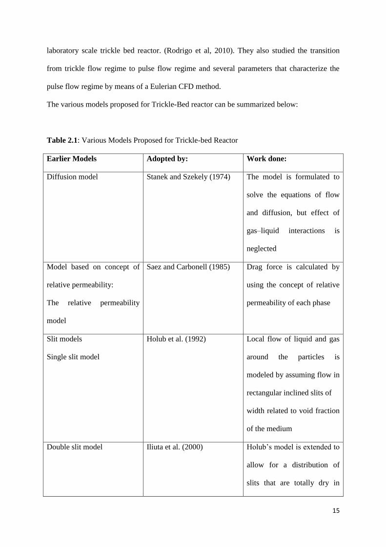
The various models proposed for Trickle-Bed reactor can be summarized below:
Table 2.1: Various Models Proposed for Trickle-bed Reactor
Earlier Models Adopted by: Work done:
Diffusion model Stanek and Szekely (1974) The model is formulated to
solve the equations of flow
and diffusion, but effect of
gas–liquid interactions is
neglected
Model based on concept of
relative permeability:
The relative permeability
model
Saez and Carbonell (1985) Drag force is calculated by
using the concept of relative
permeability of each phase
Slit models
Single slit model
Holub et al. (1992) Local flow of liquid and gas
around the particles is
modeled by assuming flow in
rectangular inclined slits of
width related to void fraction
of the medium
Double slit model Iliuta et al. (2000) Holub‟s model is extended to
allow for a distribution of
slits that are totally dry in

16
addition to slits that have
liquid flow along the wall
The interfacial force model
The fluid–fluid interfacial
force model
Attou et al. (1999) The drag force on each phase
has contribution from the
particle–fluid interaction as
well as from the fluid–fluid
interaction
Recent „CFD-based‟ models
Porous media model
(1) Anderson and Sapre
(1991)
(2) Souadnia and Latifi
(2001)
(3) Atta et al. (2007)
The drag exchange
coefficients are obtained
from the relative
permeability concept
developed by Saez and
Carbonell (1985)
k-fluid model (1) Jiang et al. (2002)
(2) Gunjal et al. (2003, 2005)
The drag exchange
coefficients are obtained
from the fluid–fluid
interfacial force model

17
CHAPTER 3
CFD METHODOLOGY IN MULTIPHASE FLOW
3.1 Computational Fluid Dynamics
CFD is a branch of fluid mechanics that deals with the study of fluid flow problems by
analysing the problem using Numerical methods and Algorithms. Navier–Stokes equations
form the fundamental basis of almost all CFD problems which define any single-phase fluid
flow. These equations can be simplified by removing terms describing viscosity to yield the
Euler equations. Further simplification, by removing terms describing vorticity yields the full
potential equations. They can be linearized to yield the linearized potential equations.
Computers are used to perform numerous calculations involved using softwares such as
Fluent, CFX. Even with simplified equations and high speed supercomputers, in many cases
only approximate solutions can be achieved. More accurate codes are written that can
accurately and quickly simulate even complex scenarios such as supersonic or turbulent
flows.
3.2 Advantages of CFD
CFD has been used extensively in last few decades because of development of fast processors
and memory storage capability of computers. This technology has widely been applied to
various engineering applications such as automobile and aircraft design, weather science,
civil engineering process engineering, and oceanography. It allows us to design and simulate
any real systems without having to design it practically. CFD analysis enables us to virtually
sneak inside the design and see how it performs. CFD gives a deep perception into the
designs hence it reduces the time of prototype production and testing, leading to a successful
glitch free design. Using CFD we can built our own desired design and have a closed look
18
inside it. A key advantage of CFD is that researchers can evaluate the performance of any
practical system on the computer without the time, expense, and they can make necessary
changes onsite. After our required design is built, we apply the fluid flow physics and
chemistry to this virtual model and correspondingly the software will output a prediction of
fluid dynamics and related physical phenomena (Kumar., 2009). Once the simulation is done
then various parameters like temperature, pressure, mass fraction etc. can be analysed. Some
of the main advantages of CFD can be summarized as:
1. It is always not possible to design a working model and test its performance and
glitches. CFD is very much helpful in this regard.
2. CFD simulation doesn‟t have a size and scale restriction. It can simulate large
capacity plant. So it avoids pilot scale simulation and the difficulties of upgrading
pilot scale plant to large scale plant.
3. It provides the much needed flexibility in changing design parameters without the
expense of onsite changes. It therefore costs less than laboratory or field experiments,
thereby allowing engineers to try and develop something alternate which will be
feasible.
4. It gives the results in a very short time as compared to the practical experiment.
5. It reduces the cost of experiment very effectively by allowing changes to variable
parameter such as flow rates, temperature

19
3.3 Governing Equations in Computational Fluid Dynamics
For all flows, conservation equations for mass and momentum are to be solved. For flows
involving heat transfer or compressibility, an additional equation for energy conservation is
solved. They are the mathematical statements of three fundamental physical principles upon
which all of fluid dynamics is based (Anderson J. D., 2009):
(1) Mass is conserved;
(2) F = ma (Newton‟s second law);
(3) Energy is conserved.
3.3.3 Boundary Conditions
For most of the fluid flow problem the basic governing equations remain the same but
boundary conditions differs according to the situations and gives shape to the solutions. The
boundary conditions as well as the initial conditions set by the user decided the fate of the
solution obtained from the governing equations.
3.4 How CFD Code Works
There are three steps for solving a CFD problem:
1. Pre-processing
2. Solver
3. Post-processing
3.4.1 Pre-processing
This is the first step in solving any CFD problem. It basically involves designing and building
the domain. It involves the following steps (Bakker. 2002):
Definition of the geometry of the region: The computational domain.
Grid generation the subdivision of the domain into a number of smaller, non-overlapping
sub domains (or control volumes or elements Selection of physical or chemical
phenomena that need to be modelled).
20
Definition of fluid properties.
Specification of appropriate boundary conditions at cells, which coincide with or touch
the boundary. The solution to a flow problem (velocity, pressure, temperature etc.) is
defined at nodes inside each cell. The accuracy of a CFD solution is governed by the
number of cells in the grid. Optimal meshes are often non-uniform: finer in areas
where large variations occur from point to point and coarser in regions with relatively
little change. Over 50% of the time spent in industry on a CFD project is devoted to
the definition of the domain geometry and grid generation. GAMBIT, T-GRID is
some of the software used in pre-processing.
3.4.2 Solver
After the geometry has been made then the next step is to do the flow calculations. CFD
solver does the flow calculations and displays the results obtained. FLUENT, FloWizard,
FIDAP, CFX and POLYFLOW are some of the types of solvers. Numerous iterations are
performed till the solution converges and the results obtained. The first step is the setting of
the under relaxation factors which are essential for the solution convergence as wrong or
improper under relaxation factors can hamper the convergence. Initialization of the solution
is also as important as setting under relaxation factors because it helps the solver to assume
some initial values required to solve the governing equations involved.
ANSYS has developed two solvers namely FLUENT and CFX. They are high precision
solvers and rely heavily on a pressure-based solution technique for broad applicability. The
CFX solver uses finite elements (cell vertex numeric), similar to those used in mechanical
analysis, to discretize the domain. In contrast, the FLUENT solver uses finite volumes (cell
cantered numeric). CFX software focuses on one approach to solve the governing equations
of motion (coupled algebraic multigrid), while the FLUENT product offers several solution
approaches (density-, segregated- and coupled-pressure-based methods) (Kumar., 2009).
21
Navier–Stokes equations form the backbone in CFD codes and its solution usually relies on a
discretization method: it means that derivatives in partial differential equations are
approximated by algebraic expressions which can be alternatively obtained by means of the
finite-difference or the finite-element method. Fluent mainly uses finite volume method for
discretization. The governing equations predicted at discrete points in the domain and several
iterations are carried till convergence as follows (Ravelli et al., 2008):
(1) Fluid properties are updated in relation to the current solution; if the calculation is at the
first iteration, the fluid properties are updated consistent with the initialized solution.
(2) The three momentum equations are solved consecutively using the current value for
pressure so as to update the velocity field.
(3) Since the velocities obtained in the previous step may not satisfy the continuity equation,
one more equation for the pressure correction is derived from the continuity equation and the
linearized momentum equations: once solved, it gives the correct pressure so that continuity
is satisfied. The pressure–velocity coupling is made by the SIMPLE algorithm, as in
FLUENT default options.
(4) Other equations for scalar quantities such as turbulence, chemical species and radiation
are solved using the previously updated value of the other variables; when inter-phase
coupling is to be considered, the source terms in the appropriate continuous phase equations
have to be updated with a discrete phase trajectory calculation.
(5) Finally, the convergence of the equations set is checked and all the procedure is repeated
until convergence criteria are met.

22
Fig. 3.1 Flowchart showing the general procedure for the simulation using Fluent (Kumar, 2009)
3.4.3 Post- processing
This is the last step and it consists of analysing the data obtained. FLUENT provides all sorts
of post processing tools and the simulation results can be interpreted and analysed using
various plots and tools. It includes:
Domain geometry and grid display
Vector plots
Line and shaded contour plots
2D and 3D surface plots
Particle tracking
Animation for dynamic result

23
3.5 CFD Approaches in Multiphase Flows
Currently there are two approaches for the numerical calculation of multiphase flows: the
Euler-Lagrange approach and the Euler-Euler approach.
1. The Euler-Lagrange Approach
2. The Euler-Euler approach
3.5.1 The Euler-Lagrange Approach
The Lagrangian discrete phases model in FLUENT follows the Euler-Lagrange approach.
The fluid phase is treated as a continuum by solving the time-averaged Navier-Stokes
equations, while the dispersed phase is solved by tracking a large number of particles,
bubbles, or droplets through the calculated flow field. The dispersed phase can exchange
momentum, mass, and energy with the fluid phase. A fundamental assumption made in this
model is that the dispersed second phase occupies a low volume fraction, even though high
mass loading (m particles ≥ m fluid) is acceptable. The particle or droplet trajectories are
computed individually at specified intervals during the fluid phase calculation. This makes
the model appropriate for the modelling of spray dryers, coal and liquid fuel combustion, and
some particle-laden flows, but inappropriate for the modelling of liquid-liquid mixtures,
fluidized beds, or any application where the volume fraction of the second phase is not
negligible (Fluent. 2006).
3.5.2 The Euler-Euler Approach
In the Euler-Euler approach, the different phases are treated mathematically as
interpenetrating continua. Since the volume of a phase cannot be occupied by the other
phases, the concept of phase volume fraction is introduced. These volume fractions are
assumed to be continuous functions of space and time and their sum is equal to one.
Conservation equations for each phase are derived to obtain a set of equations, which have
similar structure for all phases. These equations are closed by providing constitutive relations

24
that are obtained from empirical information, or, in the case of granular flows, by application
of kinetic theory. In FLUENT, three different Euler-Euler multiphase models are available:
the volume of fluid (VOF) model, the mixture model, and the Eulerian model (Fluent. 2006).
1. The VOF Model
The VOF model is a surface-tracking technique applied to a fixed Eulerian mesh. It is
designed for two or more immiscible fluids where the position of the interface between the
fluids is of interest. In the VOF model, a single set of momentum equations is shared by the
fluids, and the volume fraction of each of the fluids in each computational cell is tracked
throughout the domain. Applications of the VOF model include stratified flows, free-surface
flows, filling, sloshing, the motion of large bubbles in a liquid, the motion of liquid after a
dam break, the prediction of jet breakup (surface tension), and the steady or transient tracking
of any liquid-gas interface.
2. The Mixture Model
The mixture model is designed for two or more phases (fluid or particulate). As in the
Eulerian model, the phases are treated as interpenetrating continua. The mixture model solves
for the mixture momentum equation and prescribes relative velocities to describe the
dispersed phases. Applications of the mixture model include particle-laden flows with low
loading, bubbly flows, sedimentation, and cyclone separators. The mixture model can also be
used without relative velocities for the dispersed phases to model homogeneous multiphase
flow.
3. The Eulerian Model
It is the most complex of the multiphase models in FLUENT. It solves a set of n momentum
and continuity equations for each phase. Coupling is achieved through the pressure and
interphase exchange coefficients. The manner in which this coupling is handled depends
upon the type of phases involved; granular (fluid-solid) flows are handled differently than

25
non-granular (fluid-fluid) flows. For granular flows, the properties are obtained from
application of kinetic theory. Momentum exchange between the phases is also dependent
upon the type of mixture being modelled. FLUENT's user-defined functions allow you to
customize the calculation of the momentum exchange. Applications of the Eulerian
multiphase model include bubble columns, risers, particle suspension, and fluidized beds.
3.6 Some Multiphase Systems
Some examples of multiphase flow systems are as follows:
Fluidized bed examples: fluidized bed reactors, circulating fluidized beds.
Trickle-bed Reactor
Slurry flow examples: slurry transport, mineral processing.
Particle-laden flow examples: cyclone separators, air classifiers, dust collectors, and
dust-laden environmental flows.
Stratified/free-surface flow examples: sloshing in offshore separator devices, boiling
and condensation in nuclear reactors.
Pneumatic transport examples: transport of cement, grains, and metal powders.
3.7 Choosing a Multiphase Model
The multiphase models vary for variety of the problems. Some guidelines for deciding the
multiphase models are (Fluent., 2006):
Discrete phase model is used for bubbly, droplet, and particle-laden flows in which
the dispersed-phase volume fractions are less than or equal to 10%.
Mixture model or the Eulerian model is used for bubbly, droplet, and particle-laden
flows in which the phases mix and/or dispersed-phase volume fractions exceed 10%.
For slug flows VOF model is used.
For stratified/free-surface flows VOF model is used.
For pneumatic transport, use the mixture model for homogeneous flow or the Eulerian
model for granular flow.
26
CHAPTER 4
CFD SIMULATION OF THREE PHASE CO-CURRENT
TRICKLE-BED
4.1 Computational Flow Model
A two–dimensional Eulerian three phase model is implemented in the present work where
gas phase is treated as continuous, inter-penetrating and interacting everywhere within the
computational domain. The pressure field is assumed to be shared predominantly by air as the
liquid flow velocity is in trickle flow regime and it flow under the influence of gravity and
shear force exerted by the flowing gas. The motion of liquid and gas phase is governed by the
respective mass and momentum equations. The momentum equation for the solid phase is not
solved as it is a packed bed and each particle in the bed is assumed to be stationary. The
velocity of solid phase fixed to zero via a user interface command.
4.1.1 Equation Reformulation:
4.4.1.1 The Mass Conservation Equation
The equation for conservation of mass, or continuity equation, can be written as follows:
(αk ρk) + ∇( αk ρkUk) = 0
Where ρk is the density and αk is the volume fraction of phase k=g, l
and the volume fraction of the two phases satisfy the following condition:
αg + αl =1
4.4.1.2 Momentum Equations
For liquid phase
l αl l) + ∇ l αl lul)=- αl + ∇ αl μeff,l ∇Ul+ UlT))+ l αlg +Mi,l

27
For gas phase
g αgUg) +∇ g αgUgUg)=- αg + ∇(αg μeff,g (∇Ug+ Ug
T)) + ρg αgg +Mi,g
P is the pressure and μeff is the effective viscosity. The terms Mi,l and Mi,g of the above
momentum equations represent the interphase force term for liquid, gas and solid phase,
respectively.
4.1.2 Turbulence Modeling:
Standard k-ε model is used which include standard version of two equation model that
involves transport equations for the Turbulent Kinetic Energy k, and its dissipation rate ε.
The exact turbulence modeling equation can be derived by simplifying Navier- Stokes
equation. The k - epsilon model consists of the turbulent kinetic energy equation. Its
popularity in industrial flow and heat transfer simulations is because of robustness, economy,
and reasonable accuracy for a wide range of turbulent flows. It is a semi-empirical model,
and the derivation of the model equations relies on phenomenological considerations and
empiricism (Fluent. 2006).
Table 4.1: The model constants used for turbulence modeling
Cmu
0.09
C1- ε
1.44
C2- ε 1.92
C3- ε 1.3
TKE Prandtl Number
1
TDR Prandtl Number
1.3
Dispersion Prandtl Number
0.75

28
4.2 Problem description for the Simulation:
The problem is based on a three phase solid-liquid-gas Trickle Bed in which both liquid and
gas are flowing co-currently downward. Solid phase consists of glass bead of uniform
diameter of 6 mm in this case. The gas and liquid are sent co-currently downward from the
top with different superficial velocities. The gas velocities vary from 0.11m/s to 0.22 m/s and
liquid velocities varies from 0.003 m/s to 0.011 m/s. The velocity of both the phases lies in
the trickle flow regime.
Table 4.2 Properties of air and Water
Phases Density, Kg/m3
Viscosity, kg/m-s
Air 1.225 1.789*10-05
Water 998.2 0.001003
4.3 Geometry and Mesh
.
Figure 4.1 The unstructured grid developed for the simulation
Air, Water inlet.
1 Meter
0.194 Meter
29
GAMBIT 2.2.30 was used for making 2D rectangular geometry of width of 0.194m and
height 1m. Coarse triangular unstructured mesh size is used for the whole geometry for
better adoptability to the geometry. It consists of 3258 triangular cells, 100 -2D wall faces,
4787 -2D interior faces with 1730 nodes.
4.4 Assumptions:
Both the fluids are incompressible
The trickling flow regime is considered, i.e. the gas-liquid interaction are low, so
capillary pressure force can be neglected. We assume same pressure for both phases at
any time and space.
There is no inter-phase mass transfer
The pressure drop across the bed is due to gas phase only, as liquid undergo trickle
flow and play a little role here.
The inertial, viscous and pseudo-turbulence terms are neglected compared to the drag
force terms.
The porosity is uniform and constant.
4.5 Solution:
The above sets of equations were solved using commercial software FLUENT 6.3.26 (of
ANSYS Inc., USA) with a two-dimensional Eularian three-phase model considering the flow
domain as granular. The gas phase was treated as primary phase and liquid phase was
considered as secondary phase. At the inlet, flat velocity profile for gas and liquid phases was
assumed and implemented. No slip boundary condition was set for all the impermeable
reactor walls. At the bottom of the column, an outlet boundary condition was specified. With
mixture gauge pressure at 0 Pascal and back flow volume fraction for air is 0.Unsteady state
simulations were carried out with the time step of 0.001 s. Many workers adopted different

30
models and drag force formulation mentioned in table 2.1. In the present work Granular
multiphase flow is adopted and the drag force adopted between the three phases are
mentioned in table 4.2 (Fluent, 2006).
Table 4.3: Models used for considering Force interactions among phases.
Interactions
Model
Solid-Air
Gidaspow
Solid-Water
Gidaspow
Air- Water
Schiller-Naumann
Table 4.4 Solution Control Parameters:
Discretization Scheme First Order UPWIND
Pressure-Velocity coupling SIMPLE algorithm
Relaxation Parameters:
Pressure
Density
Momentum
Volume fraction
Body force
Turbulent Kinetic Energy
Turbulent Dissipationa Rate
0.6
1
0.2
0.2
1
0.2
0.2

31
CHAPTER 5
RESULTS & DISCUSSION
Simulation has been carried out for three-phase Trickle Bed Reactor of 1 m height and 0.194
m diameter as described in chapter-4. 6 mm glass beads have been used as the packing
material. At the top of the column uniform fluid distribution was taken considering an ideal
distributor. The simulations were performed until a quasi-steady state is reached and no
further change in the bed was observed.
.
0 sec 5 sec 10 sec 20 sec 30 sec 40 sec 50 sec 60 sec 70 sec 80 sec
Figure 5.1: Contour of volume fraction of air for air velocity 0.14 m/s and liquid velocity
0.009 m/s.
Figure 5.1 shows the change in gas phase volume fraction with time until quasi steady state is
reached. Initially an abrupt change in the volume fraction of all the gas and liquid phase were
observed. The quasi steady state was reached after 60 sec and no further change in the
contour were observed in the bed
32
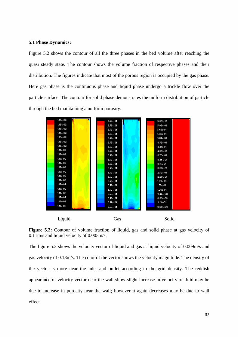
5.1 Phase Dynamics:
Figure 5.2 shows the contour of all the three phases in the bed volume after reaching the
quasi steady state. The contour shows the volume fraction of respective phases and their
distribution. The figures indicate that most of the porous region is occupied by the gas phase.
Here gas phase is the continuous phase and liquid phase undergo a trickle flow over the
particle surface. The contour for solid phase demonstrates the uniform distribution of particle
through the bed maintaining a uniform porosity.
Liquid Gas Solid
Figure 5.2: Contour of volume fraction of liquid, gas and solid phase at gas velocity of
0.11m/s and liquid velocity of 0.005m/s.
The figure 5.3 shows the velocity vector of liquid and gas at liquid velocity of 0.009m/s and
gas velocity of 0.18m/s. The color of the vector shows the velocity magnitude. The density of
the vector is more near the inlet and outlet according to the grid density. The reddish
appearance of velocity vector near the wall show slight increase in velocity of fluid may be
due to increase in porosity near the wall; however it again decreases may be due to wall
effect.

33
Water Air
Figure 5.3: velocity vector of water and Air
Figure 5.4 Radial variation of velocity of liquid at a height of Z=0.5 m at gas velocity of
0.2m/s
Radial Position, m
34
The plot in figure 5.4 shows the velocity profile of liquid along the radial direction at gas
velocity of 0.2m/s. Although uniform porosity is assumed throughout the bed still porosity
near the wall is always higher than the bulk porosity. For the same reason fluid velocity tends
to increase in that region.
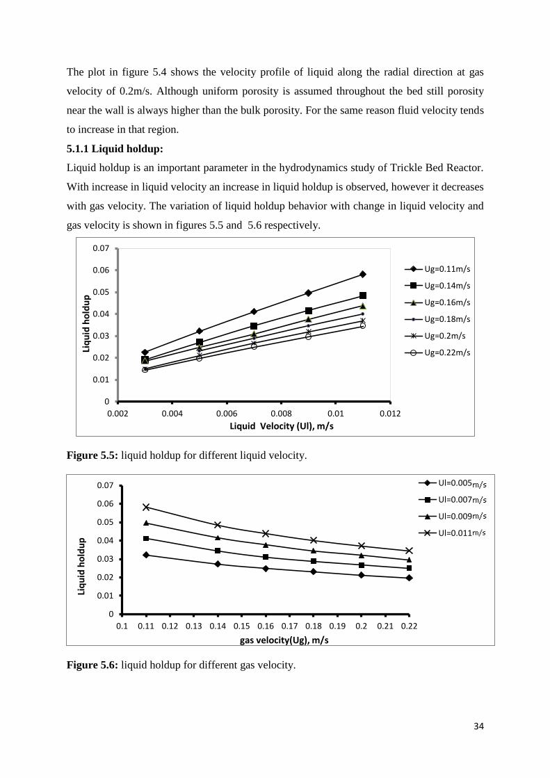
5.1.1 Liquid holdup:
Liquid holdup is an important parameter in the hydrodynamics study of Trickle Bed Reactor.
With increase in liquid velocity an increase in liquid holdup is observed, however it decreases
with gas velocity. The variation of liquid holdup behavior with change in liquid velocity and
gas velocity is shown in figures 5.5 and 5.6 respectively.
Figure 5.5: liquid holdup for different liquid velocity.
Figure 5.6: liquid holdup for different gas velocity.
0
0.01
0.02
0.03
0.04
0.05
0.06
0.07
0.002 0.004 0.006 0.008 0.01 0.012
Ug=0.11m/s
Ug=0.14m/s
Ug=0.16m/s
Ug=0.18m/s
Ug=0.2m/s
Ug=0.22m/s
Liquid Velocity (Ul), m/s
Liq
uid
ho
ldu
p
0
0.01
0.02
0.03
0.04
0.05
0.06
0.07
0.1 0.11 0.12 0.13 0.14 0.15 0.16 0.17 0.18 0.19 0.2 0.21 0.22
Ul=0.005
Ul=0.007
Ul=0.009
Ul=0.011
Liq
uid
ho
ldu
p
gas velocity(Ug), m/s

35
Radial averaged liquid holdup was calculated at ten different heights across the bed and their
cumulative averages were plotted with various flow conditions. It is an obvious observation
that liquid holdup increases with increase in liquid velocity, but it decrease with increase in
gas velocity, which is clearly observed in the figure 5.6.
The Figure 5.7 shows the liquid saturation along the length of the column. Radial averaged
liquid holdup were calculated at each 0.1 meter interval of height and plotted in the graph.
The variation of liquid holdup behavior along the height of the column for two different
liquid velocities was shown in the figure 5.7.
Figure 5.7: Liquid Holdup variation with Height of the column at liquid velocity of 0.003m/s
and 0.011m/s.(gas velocity= 0.2m/s)
In both cases the liquid holdup is more at the bottom part of the column. The gradient is more
prominent for lower liquid velocities and almost equal distribution is observed at higher
liquid velocities. The liquid saturation shows a gradient when operated at lower liquid
velocity of 0.003m/s however it shows a flat profile along the length of the column when the
velocity is increased to 0.011m/s.
0.0149
0.01491
0.01492
0.01493
0.01494
0.01495
0.01496
0 0.2 0.4 0.6 0.8 1
Liq
uid
Ho
ldu
p, α
L
Height of The column(Z), m
Ul=0.003m/s
0.03638
0.03639
0.0364
0.03641
0.03642
0.03643
0.03644
0.03645
0.03646
0 0.2 0.4 0.6 0.8 1
Liq
uid
Ho
ldu
p, α
L
Height of The column(Z), m
Ul=0.011m/s

36
figures 5.8(a) and 5.8 (b) show the radial distribution of liquid at different height of the
column. Liquid holdup along the cross section were observed at three different height i.e
0.25m, 0.5m, 0.75m for two different gas velocities. In both the cases the liquid saturation is
uniform at the distributor and gradually the liquid saturation increases at the center and tends
to decrease near the wall.
Comparison of the two sets of figure revels that the variation in liquid saturation along the
diameter is more in case of lower gas velocity i.e. 0.11m/s but the variation is not so
prominent at higher gas velocity i.e. 0.20 m/s.
Figure 5.8 (a) Radial Averaged Liquid Holdup variation along the diameter of the column at
different height at gas velocity of 0.11m/s and liquid velocity 0.009 m/s
Figure 5.8(b) Radial Averaged Liquid Holdup variation along the diameter of the column at
different height at gas velocity of 0.20m/s and liquid velocity 0.009 m/s.
0.04833
0.048335
0.04834
0.048345
0.04835
0.048355
0.04836
0 0.02 0.04 0.06 0.08 0.1 0.12 0.14 0.16 0.18 0.2
Height Z=0.25
Height Z=0.5
Heght z=0.75
Radial Position, m
Liq
uid
Ho
ldu
p
Height Z=0.25m
Height Z=0.5m
Height Z=0.75m
0.03155
0.031555
0.03156
0.031565
0.03157
0.031575
0.03158
0 0.02 0.04 0.06 0.08 0.1 0.12 0.14 0.16 0.18 0.2
Heigt Z=0.25
Height Z=0.5
Height Z=0.75
Height Z=0.5m
Height Z=0.75m
Height Z=0.25m
Radial Position, m
Liq
uid
Ho
ldu
p

37
5.1.2 Gas Holdup
Gas holdup is obtained as mean area-weight average of volume fraction of the gas phase at
sufficient number of axial positions in the Trickle bed reactor. The variation of gas holdup
with superficial liquid velocity obtained from CFD simulation is shown in figure 5.9. The
Graph shows a decrease in gas holdup with liquid velocity. The experimental data form
Gunjal et al (2005) and other workers also shows the similar tendency of the gas holdup in
literature
Figure 5.9: Gas holdup for different liquid velocity
Figure 5.9: Gas holdup for different gas velocity
0.935
0.94
0.945
0.95
0.955
0.96
0.965
0.97
0.975
0.98
0.985
0.99
0.002 0.004 0.006 0.008 0.01 0.012
Ug=0.11m/s
Ug=0.14m/s
Ug=0.16m/s
Ug=0.18m/s
Ug=0.2
Ug=0.22m/s
Gas
Ho
ldu
p
Liquid velocity (Ul), m/s
0.9350.94
0.9450.95
0.9550.96
0.9650.97
0.9750.98
0.985
0.1 0.12 0.14 0.16 0.18 0.2 0.22
Ul=0.005m/s
Ul=0.007m/s
Ul=0.009m/s
Ul=0.011m/sGas
Ho
ldu
p
Gas Velocity (Ug) m/s
38
When gas velocity is increased the gas holdup in the trickle bed reactor increases. This
tendency is shown in figure 5.9; it may be because more amount of volumetric gas is flowing
when gas velocity is increased. Since the flow domain has a constant porosity, the phase
holdup of gas and solid are inter-dependent.
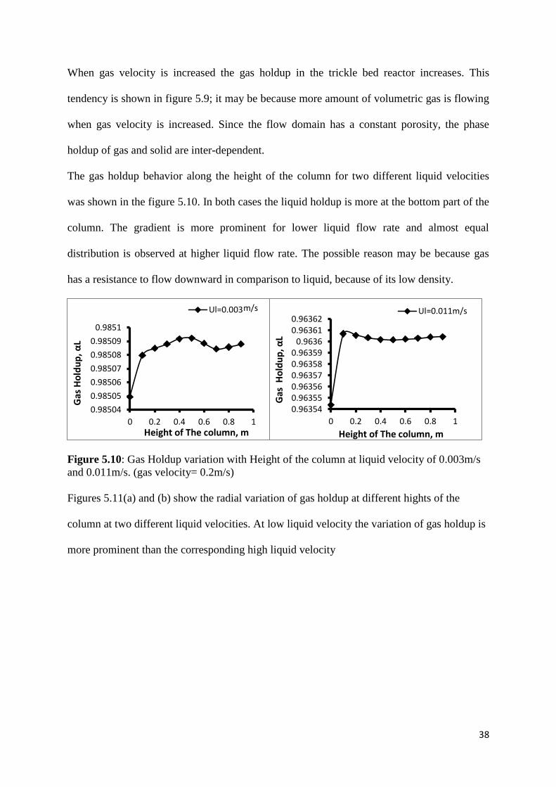
The gas holdup behavior along the height of the column for two different liquid velocities
was shown in the figure 5.10. In both cases the liquid holdup is more at the bottom part of the
column. The gradient is more prominent for lower liquid flow rate and almost equal
distribution is observed at higher liquid flow rate. The possible reason may be because gas
has a resistance to flow downward in comparison to liquid, because of its low density.
Figure 5.10: Gas Holdup variation with Height of the column at liquid velocity of 0.003m/s
and 0.011m/s. (gas velocity= 0.2m/s)
Figures 5.11(a) and (b) show the radial variation of gas holdup at different hights of the
column at two different liquid velocities. At low liquid velocity the variation of gas holdup is
more prominent than the corresponding high liquid velocity
0.98504
0.98505
0.98506
0.98507
0.98508
0.98509
0.9851
0 0.2 0.4 0.6 0.8 1
Ul=0.003
Gas
Ho
ldu
p, α
L
Height of The column, m
0.963540.963550.963560.963570.963580.96359
0.96360.963610.96362
0 0.2 0.4 0.6 0.8 1
Ul=0.011m/s
Gas
Ho
ldu
p, α
L
Height of The column, m
m/s

39
Figure 5.11(a) Gas Holdup variation along the diameter of the column at different height at
gas velocity of 0.20m/s and liquid velocity 0.003 m/s
Figure 5.11(b) Gas Holdup variation along the diameter of the column at different height at
gas velocity of 0.20m/s and liquid velocity 0.009 m/s
But in both the cases it is observed that the gas tend to accumulate at the center as well as
near to the wall leaving a annular region for liquid. This kind of liquid-gas mal-distribution is
a problem in industrial Trickle bed reactor, which reduces the efficiency of the reactor.
0.98507
0.985075
0.98508
0.985085
0.98509
0.985095
0.9851
0 0.02 0.04 0.06 0.08 0.1 0.12 0.14 0.16 0.18 0.2
Radial Position, m
Gas
Ho
ldu
p
0.96842
0.968425
0.96843
0.968435
0.96844
0.968445
0.96845
0 0.02 0.04 0.06 0.08 0.1 0.12 0.14 0.16 0.18 0.2
Radial Position, m
Gas
Ho
ldu
p
Height Z=0.25m
Height Z=0.5m
Height Z=0.75m
Height Z=0.25m
Height Z=0.5m
Height Z=0.75m

40
5.1.3 Pressure Drop:
Pressure drop is another important hydrodynamics property of a trickle bed-reactor. Pressure
drop in the bed were predicted by taking different flow conditions and have been represented
graphically in the following figures.
Figure 5.12: Variation of Pressure drop per unit length with liquid velocity at different
superficial gas velocities.
Pressure drop in a trickle bed will be different in pre-wetted and non-pre-wetted bed
condition. For an ideal assumption pre-wetted bed condition is assumed where capillary force
is neglected.
Figure 5.13: Graph showing Pressure drop along axial length of the bed.
5000
7000
9000
11000
13000
15000
17000
19000
21000
23000
25000
0.002 0.004 0.006 0.008 0.01 0.012
Ug=0.11 m/s
Ug=0.14m/s
Ug=0.16m/s
Ug=0.18 m/s
Ug=0.2m/s
Ug=0.22 m/s
PR
ESSU
RE,
Pa
LIQUID SUPERFICIAL VELOCITY, m/s
y = 16798x + 8.2175
0
5000
10000
15000
20000
0 0.2 0.4 0.6 0.8 1
Pre
ssu
re D
rop
, Pa
Height of the column, m
VG=0.18m/s,VL=0.007m/s

41
Figure 5.10 shows the pressure gradient across the bed. Radial averaged pressure drop were
predicted at different places in the column and plotted against height. The slope of the linear
variation can be represented as pressure drop per unit length. Similarly pressure drop for all
the flow conditions in the experiment were predicted and they were plotted in figure 5.9.
Sauadnia et al (2001) also predicted the axial pressure drop variation for gas and found the
same profile at different liquid and gas flow velocities.
Figure 5.14: Radial-Averaged Pressure drop along the diameter of the column at different
height at gas velocity of 0.2m/s and liquid velocity 0.003 m/s
The Figure 5.11 shows the radial pressure drop variation at three different heights. The radial
pressure variation is not of much concern until the operating condition of the reactor is not at
the boiling condition of the fluid. Such an oscillating profile for pressure drop along the radial
direction was also predicted by Rodrigo et al (2009).
2000
3000
4000
5000
6000
7000
8000
0 0.02 0.04 0.06 0.08 0.1 0.12 0.14 0.16 0.18 0.2
Radial Position, m
Pre
ssu
re D
rop
, Pa
Height Z=0.25m
Height Z=0.5m
Height Z=0.75m

42
5.2 Comparison with the literature data:
Many scholars have studied trickle bed under different operating conditions. The present
work is compared with the work of Sunderesan et al (1991), Gunjal et al (2005) and
Atta et al (2007).
Table 5.1 The different experimental setup for the data compared.
Source Bed
Diameter
Bed
Length,
m
Particle
Diameter,
Dp
D/Dp
ratio
Bed
porosity
Gas
velocity,
m/s
Liquid
velocity, m/s
Sunderesan et
al, 1991
0.1650 1.49 0.003 55 0.37 0.22 0.002 -
0.008
Gunjal et al
2005
0.114 1 0.006 19 0.37 0.22 0.0017-
0.0092
Atta et al, 2007 0.2 1 -------- ------ 0.37 0.22 0-0.008,,
Present work 0.194 1 0.006 32.33 0.37 0.22 0.003-
0.011
Figure 5.15: The Pressure drop Comparison with Previous works
0
5000
10000
15000
20000
25000
30000
0 0.002 0.004 0.006 0.008 0.01 0.012
arnab atta et al
Sundaresan et al
gunjal et al
Present work
Liquid Velocity, m/s
Pre
ssu
re D
rop
, Pa/
m

43
Gunjal et al (2005) obtained the drag exchange coefficients from the interfacial force model
developed by Attou et al (1999). Atta et al (2007) obtained the drag exchange coefficients
from relative permeability concept developed by Saez and Carbonell (1985). In the present
work Multiphase granular flow model has been adopted and the corresponding drag force
model has been mentioned in table 4.2.
The results have a fair agreement with the work of Arnab Atta et al (2007). The deviation
occurs because of idealistic assumption and negligence of capillary force and porosity
distribution. Equations for capillary force can be modeled and implemented for greater
accuracy.
The liquid holdup at different radial positions at gas velocity 0.11m/s and liquid velocity
0.003m/s has been compared with that of Jiang et al (2001) at same gas velocity and liquid
velocity 0.001m/s and found to be agreeing well. variation of liquid holdup in radial direction
is more in Jiang et al, because of his defined radial porosity profile.
Figure 5.16: comparison of liquid holdup of along the diameter of the column at a height
0.879 Z at gas velocity of 0.11m/s with previous work
0.020.0205
0.0210.0215
0.0220.0225
0.0230.0235
0.024
0 0.2 0.4 0.6 0.8 1
Jiang et al
Present work
Radial Position, (x/D)
Liq
uid
Ho
ldu
p
44
CHAPTER 6
CONCLUSIONS
CFD simulations of three phase trickle-bed reactor were carried out by employing Eulerian-
Eularian approach for different operating conditions and flow conditions (Gas velocity
0.11m/s to 0.22m/s and liquid velocity of 0.003m/s to 0.011m/s). Liquid holdups, Gas
holdups and Pressure drop which are important hydrodynamics parameter were studied. The
results have been represented in graphical form and analysed.
The main conclusions that can be drawn are:
Liquid holdup increases with increase in liquid velocity and decrease with gas
velocity. When liquid velocity was increased from 0.003 to 0.011 m/s the liquid
holdup increased from 0.021 to 0.006 for gas velocity 0.11m/s. But on increasing the
gas velocity from 0.11m/s to 0.22m/s liquid holdup decreased from 0.06 to 0.03.
Gas holdup increases with increase in gas superficial velocity and decreases with
increase in liquid superficial velocity. On increasing the gas velocity from 0.11m/s to
0.2 m/s gas holdup increased from 0.94 to 0.96 at liquid velocity of 0.011m/s. when
liquid velocity is increased from 0.003m/s to0.011m/s gas holdup decreased to 0.94
from 0.978 at gas velocity of 0.11m/s.
Radial distribution of liquid is found to be better at higher gas velocity in compared to
lower gas velocity. At higher gas velocity of 0.2m/s the radial variation of liquid
holdup is nearly flat, but at lower gas velocity of 0.11m/s the radial liquid holdup
variation is almost hyperbolic.

45
The liquid saturation is not uniform throughout the length of the column. The
saturation is more at the bottom of the column. However the gradient of saturation of
liquid along the height decreases with increase in liquid velocity. A reverse behaviour
is observed in case of Gas holdup.
Pressure drop across the bed increases with increase in both gas and liquid velocities.
Increase in liquid velocity from 0.003m/s to 0.011m/s increases pressure drop from
7 KPa to 15 KPa at gas velocity of 0.11m/s. Similarly when gas velocity is increases
from 0.11m/s to 0.22m/s pressure increases from 15KPa to 25KPa at liquid velocity
of 0.011m/s. Increase in gas velocity has a greater impact on pressure drop.
The pressure gradient along the bed height is almost linear. At gas velocity of 0.18m/s
and liquid velocity of 0.007 m/s the pressure gradient along the axial direction of bed
was determined to be linear with 16798 Pa/m. Radial pressure variation is not
prominent.
The results have been compared with the work of Atta et al and Jiang et al and found
to be agreed well.
46
REFERENCES
Al-Dahhan, M. H., Khadilkar, M. R., Wu, Y., and Dudukovic, M. P., 1998. Prediction of
Pressure Drop and Liquid Holdup in High-Pressure Trickle-Bed Reactors. Ind. Eng. Chem.
Res., 37, 793-798.,
Al-Dahhan, Muthanna, H., Larachi, F., Dudukovic, M. P., and Laurent, A., 1997. High-
Pressure Trickle-Bed Reactors: A Review. Ind. Eng. Chem. Res. 36, 3292-3314.
Anderson, D.H., Sapre, A.V. Trickle-bed reactors flow simulation, 1991. A.I.Ch.E. Journal.
37, 377–382.
Anderson, J. D., Computational Fluid Dynamics- An Introduction, Third Edition.
Attou, A , Boyer, C., Ferschneider, G., 1999.Modelling of the hydrodynamics of the co-
current gas-liquid trickle flow through a trickle-bed reactor. Chemical Engineering Science,
54, 785-802
Atta, A., Roy, S., Nigam, Krishna, D.P.,2007. Investigation of liquid mal-distribution in
trickle-bed reactors using porous media concept in CFD. Chemical Engineering Science. 62,
7033–7044.
Bakker, A, 2002. Fluent introductory notes, Fluent Inc., Lebanon
Boyer, C., Volpi, C., Ferschneider, G., 2007. Models for pressure drop and liquid holdup,
formulation and experimental Validation. Chemical Engineering Science, 62, 7026 – 7032.
Ellman, M.J.,Midoux, N., Laurent, A., and Charpentier, J. C.,1988. A new, improved
pressure drop correlation for trickle-bed Reactors. Chemical Engineering Science, 43, 2201-
2206.
Fluent 6.3 Documentation, 2006. Fluent Inc., Lebanon

47
Gianetto, A., Baldi, G., Specchia, V., Sicardi, S., 1978. Hydrodynamics and solid-liquid
contacting effectiveness in trickle-bed reactor. A.I.Ch.E. Journal, 24, 1087-1104.
Gunjal, Prashant, R., Kashid, M. N., Ranade, V. V., and Chaudhari, R. V., 2005.
Hydrodynamics of Trickle-Bed Reactors: Experiments and CFD Modelling. Ind. Eng. Chem.
Res., 44, 6278-6294.
Holub, R. A., Dudukovic, M. P. And Ramachandran, P.A., 1992. A phenomenological model
for pressure drop, liquid holdup, and flow regime transition in gas-liquid trickle flow.
Chemical Engineering Science, 47, 2343-2348.
Iliuta, I., Larachi, F., Al-Dahhan, M.H., 2006. Double-slit model for partially wetted trickle
flow hydrodynamics. A.I.Ch.E. Journal. 46, 597–609.
Jiang, Y., Khadilkar, M. R., Al-Dahhan, M. H., Dudukovic M. P., 2001. CFD modelling of
multiphase flow distribution in catalytic packed bed reactors: scale down issues. Catalysis
Today 66, 209–218
Kumar, A., 2009. CFD Modelling of Gas-Liquid-Solid Fluidized Bed. B. Tech. Thesis,
NIT,Rourkela, India.
Kundu, A., Saroha, A. K., Nigam, K. D. P, 2001. Liquid distribution studies in trickle-bed
reactors, Chemical Engineering Science. 56, 5963–5967.
Langea, R., Schuberta, M., Dietrichb, W., Grünewaldb, M., Unsteady-state operation of
trickle-bed reactors, 2004. Chemical Engineering Science. 59, 5355 – 5361
Lappalainen, K., Alopaeus, V., Manninen, M. and Aittamaa, J, 2008. Improved
Hydrodynamic Model for Wetting Efficiency, Pressure Drop, and Liquid Holdup in Trickle-
Bed Reactors, Ind. Eng. Chem. Res., 47, 8436–8444.
Latifi, M. A., Midoux, N. and Storck, A.,1992. Hydrodynamic study of a trickle-bed reactor
By means of micro-electrodes: Analysis of the probability densities, Chemical Engineering
Science. 47, 2331-2336.

48
Maiti, R., Khanna, R., and Nigam, K. D. P., 2006. Hysteresis in Trickle-Bed Reactors: A
Review. Ind. Eng. Chem. Res., 45, 5185-5198.
Mao, Z., Hong-bin, X. H., 2001. Experimental Investigation of Pressure Drop Hysteresis in a
Concurrent Gas–Liquid Up flow Packed Bed. The Chinese Journal of Process
Muthanna, H. Al-Dahhan, Larachi, F., Dudukovic, M. P., and Laurent, A., 1997. High-
Pressure Trickle-Bed Reactors: A Review. Ind. Eng. Chem. Res. 36, 3292-3314.
for process intensification, Proceedings of European Congress of Chemical Engineering
(ECCE-6) Copenhagen.
Ravelli, S.,Perdichizzi, A., Barigozzi, G., 2008. Description, applications and numerical
modeling of bubbling fluidized bed combustion in waste-to-energy plants, Progress in Energy
and Combustion Science 34, 224–253.
Richard, M. P., Phillip, C., William, Y. C., and Marcus, S. D., 2000. A Numerical Model for
Trickle Bed Reactors. Journal of Computational Physics. 165, 311–333
Rodrigo, Lopes, J. G., Quinta-Ferreira, R. M., 2010. Assessment of CFD-VOF Method for
Trickle-Bed Reactor Modeling in the Catalytic Wet Oxidation of Phenolic Wastewaters, Ind.
Eng. Chem. Res., 49, 2638–2648
Rodrigo, Lopes, J. G. and Quinta-Ferreira, M. R., 2007. Multiphase CFD Modelling of
Trickle-Bed Reactor Hydrodynamics, Proceedings of the World Congress on Engineering
and Computer Science.
Saroha, A. K., Nandi, I., 2008.Pressure drop hysteresis in trickle bed reactors. Chemical
Engineering Science, 63, 3114 – 3119.
Satterfield C.N., 1975. Trickle-bed reactors. A.I.Ch.E. Journal. 21, 209–228.
Ookawara, A. S., Kuroki, A., 2007. High-fidelity DEM-CFD modelling of packed bed reactors
Engineering.1,1476-8186.

49
Sie, S.T., Krishna R., 1998. Process Development and Scale Up: III. Scale-up and scale-down
of trickle-bed process. Rev. Chem. Eng. 14(3), 203-252.
Souadnia, A., Latifi, M. A., 2001. Analysis of two-phase flow distribution in trickle-bed
reactors. Chemical Engineering Science 56, 5977–5985.
Stanek, V., Szekely, J. Three-dimensional flow of fluids through non-uniform packed beds.
A.I.Ch.E. Journal. 1974. 20, 974–980.
Sundaresan, S. Michael, J. S., 1991. Effect of boundaries on trickle bed hydrodynamic.
A.I.Ch.E. journal. 37, 1237-1241.
Trivizadakis, M., Giakoumakis, D. and Karabelas, A., 2004. The effect of packing particle
type on fluid mechanical characteristics of trickle bed reactors. Workshop of CPERI.
Wammes, W. J. A, Middelkamp, J., Huisman, W. J., and Westerterp, K. R., 1991.
Hydrodynamics in a Cocurrent Gas-Liquid Trickle Bed at Elevated Pressures. A.I.Ch.E
Journal. 37, 1849–1862.
Wammes, W. J. A., Mechielsen, S. J., and Westerterf, K. R., 1990. The transition between
trickle flow and pulse Flow in a cocurrent gas-liquid trickle-bed Reactor at elevated
pressures, Chemical Engineering Science, 45, 3149-3158.
Wang, R., Mao, Z. and Chen, J., 1995. Experimental and theoretical studies of pressure drop
hysteresis in trickle bed reactors., chemical engineering science, 50, 2321-2328,
www.wikipedia.org/trickle-bed_reactor