5th High Performance Yacht Design Conference Auckland, 10-12 March, 2015

HYDRODYNAMIC ASPECTS OF TRANSOM STERN OPTIMIZATION

Michal Orych1, michal@flowtech.se Lars Larsson2, lars.larsson@chalmers.se

Abstract. In this work an explanation for an optimum transom size is proposed which takes into account the hull shape between the midship and the transom. A systematic stern modification is performed to study the influence of the shape of waterlines and buttocks on the resistance components. The aft body of a hull is designed in a way that gives a possibility to separate the effects of waterline and buttock curvature and to study their effect on the flow. The Froude numbers are chosen to provide information for wetted- as well as dry-transom conditions. To evaluate the performance of the hulls the SHIPFLOW steady state Reynolds Averaged Navier-Stokes (RANS) code with a Volume of Fluid (VOF) surface capturing method is used in combination with the k-ω SST turbulence model. The code was first thoroughly validated for a transom stern hull. The paper focuses on hydrodynamic and hydrostatic resistance components of the transom and of the rest of the hull. Physical explanations are given for the effects of the aft body hull lines. The transom size, waterline curvature and rocker effects are analysed. The results show that the optimum transom size depends on the balance between the hydrostatic and hydrodynamic force components and the explanation for this is also given.

1 FLOWTECH International AB, Gothenburg, Sweden 2 Professor, Department of Shipping and Marine Technology, Chalmers University of Technology, Gothenburg, Sweden

NOMENCLATURE At/Ax Transom area divided by maximum section

area Rt/W Total resistance divided by weight

displacement, referred in the paper as a total resistance

Rp_hd/W Hydrodynamic pressure resistance divided by weight displacement, referred in the paper as a hydrodynamic resistance

Rp_hs/W Hydrostatic pressure resistance divided by weight displacement, referred in the paper as a hydrostatic resistance

Tt/Tc Transom submergence divided by hull draft

tz Transom centroid submergence

1. INTRODUCTION

This work is a development of a study on sailing yacht transom sterns carried out at Chalmers University of Technology [1] and later described in the paper proposed for the 5th High Performance Yacht Design conference [2] where the influence of a transom size and shape on a yacht performance was investigated using Computational Fluid Dynamics (CFD) and a Velocity Prediction Program (VPP). The need for a better understanding of the physics of the stern flow is the primary reason to extend the work and deepen the subject.

Modern sailing yachts easily reach high displacement and semi-displacement speeds, thus may benefit from larger transoms. In a hull design process the transom size is most often based on general guidelines and experience of the individual design office. There is very little explanation in the literature as to the reasons why the optima exist and why the transom should be larger for faster vessels. The works of [3] and [4] discuss the formation of the hollow behind the transom which

virtually extends the hull length and in this way creates a favourable change in the Froude number.

In this work the focus is put on the analysis of the resistance components and their physical explanation. An idea that the optimum transom size is directly linked to a balance between the base drag, transom hydrostatic resistance and aft body waterline and buttock curvatures and their effect on hydrodynamic drag is explored. A special purpose hull was designed with section shapes which help to differentiate the effects of buttocks and waterlines. The transom width and draught was then systematically varied and the changes in the flow and resulting forces acting on the hull were analysed.

2. NUMERICAL METHOD

The solver is based on the steady RANS equations. The closure terms are modeled with the Menter k-ω SST turbulence model. The model is valid all the way to the solid walls, so there is no need for wall functions. Also no special treatment for the turbulence modeling was applied near the free surface interface. More details on the solver and the turbulence model can be found in [5] and [6].

In addition to the RANS and turbulence model equations, a water fraction transport equation is introduced. A scalar function describes the amount of water in each cell of the computational domain and takes values from 0 in the air to 1 in the water. The intermediate values indicate the location of the free surface. For detailed free surface solution the transition band has to be thin, which usually means around 3 cells. Therefore, the discretization scheme needs to be able to represent a step discontinuity in the best possible manner.

The partial differential equations are discretized to algebraic equations with the Finite Volume Method (FVM). The averaged values in each cell volume surrounding the centers are calculated from face fluxes. The variations of the flow properties between the cells

247

are approximated with appropriate differencing schemes which are chosen to support the physical behavior of the flow. The convective flux discretization is based on the first order Roe type flux difference splitting algorithm, [7]. Higher order accuracy is achieved by the explicit defect correction with flux extrapolation based on the work presented by [8], which stems from the [9] formulation. High resolution schemes are composed by applying limiters to the correction terms and blending of basic schemes. The limiter functions select an appropriate correction term based on the relations of flux differences in the computational stencil. High resolution composite schemes have been developed to overcome problems with non-physical oscillations and overshoots of a solution.

All convective terms use the Monotonic Upwind Scheme for Conservation Law (MUSCLE) scheme, except the water fraction equation for which Switching Techniques for Advection and Capturing (STACS) [10] was applied. This blended scheme is switching, between the STOIC, high resolution scheme and the SuperBee, compressive scheme [11]. The blending depends on the angle between the normal to the interface and the normal to the cell face. When the interface is parallel to the face the compressive scheme is used. The blending function allows for rapid changes away from the compressive to the high-resolution scheme when the interface is not along the grid direction.

A source balancing method is used to introduce gravity, [12], [13]. The body forces that arise from the gravity are incorporated into the approximate Riemann solver and the Roe type discretization. The pressure gradient due to gravity is subtracted from the input states for the solver. Thus, only the perturbations from the steady state are seen, not the large hydrostatic pressure gradient that would otherwise create spurious accelerations of the fluid particles due to strong coupling of pressure and velocity. The boundary conditions are implemented using two layers of ghost cells [7]. The initial conditions are specified as uniform flow with an undisturbed free surface and an approximate boundary layer profile. The hydrostatic pressure and void fraction fields are prescribed accordingly.

A local artificial time-step is added to the equations and the discrete coupled equations are solved with the Alternating Direction Implicit (ADI) method. For each sweep a local artificial time-step is calculated based on the CFL and von Neumann numbers.

3. VALIDATION

3.1 Test case

For the validation a planing hull designed by SSPA Sweden AB was selected. The choice was dictated by the availability of the experimental data for a wide range of speeds. The main particulars of the hull are given in Table 1. Figure 1 shows a general perspective view of the shape.

Table 1. Main particulars of validation case.

Length LOA [m] 2.475

Length LWL [m] 2.264

Draft Tc [m] 0.131

Beam B [m] 0.620

LCB position [% of LPP aft of midship] 9.680

Figure 1. Perspective view of planing hull.

3.2 Computational setup and results

H-O multi-block, structured grids were generated for one side of the hull. The cell density in the longitudinal direction was increased close to the transom and bow as large pressure gradients can be expected in these regions. There is also a refinement in the girthwise direction in the vicinity of the free surface, see Figure 2. In the normal direction the grid is highly stretched towards the hull to satisfy the turbulence model requirement for y+ which should be around 1. In total, the flow domain contains about 4M cells.

The computations were performed for a range of Fn between 0.2 and 1.6. This in model scale corresponds to Rn from 1.9*106 to 15.0*106. The hull sinkage and trim is prescribed and corresponds to the towing tank measurements.

The resistance predictions agree very well with the measurements. The average error in the range from Fn 0.3 – 0.6, which is used in the further investigations is about 2%, Figure 3. A very characteristic peak in the Ct curve at a speed when the transom clears is also accurately captured, Figure 4.

Figure 2. Surface mesh.

248

Figure 3. Comparison of computed and measured resistance curves

Figure 4. Comparison of computed and measured resistance coefficient (Ct) curves

4. TEST HULL

4.1 Hull design

In this work an explanation for an optimum transom size is proposed which takes into account the hull shape between the midship and the transom. A systematic stern modification is performed to study the influence of the shape of waterlines and buttocks on the resistance components.

Figure 5. Profile and half-breadth plan of test hull. Base hull (black, 1), example of narrow and deep transom variant (blue, 2).

Figure 6. Body plan of base hull

Figure 7. Example transom variants; base (1, black), wide and deep (2, green), narrow and deep (3, blue), narrow and shallow(4, red).

The aft body of a hull was designed in a way that gave the possibility to separate the effects of waterline and buttock curvature and to study their effect on the flow, see Figure 5. A rectangular section shape with a relatively small bilge radius was used, Figure 6. For a specific parameter combination, the shape of the waterline and keel line can be varied simultaneously without changing the volume distribution to decouple the effects of the longitudinal centre of buoyancy and prismatic coefficient. In order to simplify the hull generation procedure only two parameters were used which control the transom width and the transom immersion respectively, Figure 7. The Froude numbers are chosen to provide information for wetted- as well as dry-transom conditions.

4.2 Grids and computational setup

The knowledge gained during the validation process as well as previously performed verification exercises [14] was applied throughout the investigation of the transom size. The same grids and solver settings were used to get reliable results. The trim and sinkage were computed using a potential flow method. The accuracy of the code was earlier investigated on a R/V Athena [15] with good results up to Fn of 0.5 but with a slight under prediction of the sinkage and trim at 0.6.

4.3 Investigated cases

For this study a 4x4 matrix of systematically varied aft body lines was generated. The transom submergence, Ttr, ranges from 0.125 to 0.5 Tc and the width Btr is from 0.5 to 1.0 B. The consistency of the hull lines is prioritized over the LCB, CP and CB to avoid unrealistic forms. These form parameters are considered to be a result of desired hull lines and transom size. The hull parameters are given in Table 2. Table 2. Parameters of test hulls.

LWL/BWL 4.80 BWL/Tc 6.25

LWL/∇c1/3 5.8 – 6.1

LCB [%] 2.7 – 6.8

LCF [%] 6.7 – 9.0 CB 0.73 – 0.81

CP 0.72 – 0.82

CFD simulations for all hull variants are performed for Fn from 0.25 to 0.70 at a model scale Rn. To get a better understanding of the flow and to be able to separate the

1 4

2 3

2 1

249

effects of hull attitude both fixed hull and free sinkage and trim cases are investigated.

5. RESULTS AND DISCUSSION

The analysis of the results is split into two major parts. The first one focuses on the effects of the aft body shape on the resistance for a fixed hull where the trim and sinkage are fixed. The second part deals with the additional consequences of the trim and sinkage. In each of these parts flow regimes with wet and dry transom are distinguished.

5.1 Resistance decomposition of hull with fixed attitude

In this part of the work the differences between the hulls originate solely from the aft body shape. There is no influence of trim and sinkage as the hull attitude is fixed. The pressure distribution and wave elevation in the forebody part are confirmed to be identical for individual Froude numbers. Therefore the effects of aft body shape are isolated and suitable for detailed analysis.

5.1.1 Low Froude number – wet transom

At Fn of 0.30 the transom is wet. The hydrostatic pressure resistance increases with increased transom depth. A larger streamline curvature at the transom edge for deeper submergence leads to a lower pressure on the transom surface and consequently lowered water level behind it, see Figure 8. This gives rise to a larger hydrostatic imbalance.

Figure 8. Free surface elevations behind the transom with different submergence viewed from aft. Transom edges are shown in colored solid lines and dashed lines correspond to free surface elevations. The black dashed line indicates undisturbed free surface level.

The hydrodynamic pressure resistance increases with increased depth as well. The larger streamline curvature at the transom edge for a deeper submergence leads to lower pressure on the wet part of the transom and therefore, to an increase in the hydrodynamic transom resistance, corresponding to the base drag in aerodynamic literature. The lower pressure is combined with a larger area which amplifies the effect. This is partially offset by the lower buttock curvature for larger transoms creating a less negative pressure that acts on a surface with a normal pointing less aft.

The hydrostatic pressure resistance increases with width. There is an increased transom drag due to a larger area of lost wetted transom part, see Figure 9. This

originates from the lowered pressure on a wide bottom edge and more curved streamlines leaving the transom along the waterlines, Figure 10. Additionally at this Froude number the narrower transoms show higher water level at the transom due to the wave formation at the aft shoulder as a result of curved waterlines, Figure 10.

Figure 9. Free surface elevations behind the transom with different widths viewed from aft. Transom edges are shown in colored solid lines and dashed lines correspond to free surface elevations. The black dashed line indicates undisturbed free surface level.

Figure 10. Schematic representation of flow around two different transom designs; top view of aft part.

The hydrodynamic pressure resistance has a maximum for medium width. There seems to be a trade-off between pressure resistance changes due to waterline curvature, flow around the bilge (with high curvature) and the hydrostatic and hydrodynamic resistance of the transom. Additionally there is a contradictory effect from the smaller area of the bottom for a narrow transom and the suction effect created by the sides with a normal pointing aft. The waterline curvature at the aft shoulder generates a pronounced wave system, see Figure 10.

5.1.2 Intermediate and High Froude number – dry transom

For the investigated hull the transom becomes dry to a large extent at a Fn of 0.40. The hydrostatic resistance replaces the hydrodynamic component on the transom surface. The wide transoms are more beneficial partly since the area centroid is closer to the undisturbed water level which lowers the hydrostatic resistance. From this

wide

narrow

250

Fn upwards the optimum transom size depends on the balance between benefits of straighter waterlines and buttocks and the penalty that comes with it when the transom area is larger and the loss of hydrostatic pressure increases.

At Fn of 0.50 a dry transom condition is fully developed.

The hydrostatic pressure resistance increases with increased transom depth and width. When the transom is dry and the hull sides are parallel the hydrostatic resistance of the aft body is equal to the hydrostatic pressure loss at the ventilated transom and is equal to

tt Azg . This means that we can expect a constant

hydrostatic resistance for a given transom size even when the speed of the vessel increases. This indicates that the transom resistance penalty for larger transom area might be balanced out by the decrease in hydrodynamic resistance component for aft bodies with less curved buttocks and waterlines.

At higher Fn the advantage of having straighter waterlines and buttocks is very clear. The hydrodynamic pressure resistance decreases with increased transom depth and width. The pressure coefficient is higher when the curvature is decreased and at the same time the surface normal is pointing less aft.

The optimum depends on the balance between the increase in the hydrostatic transom resistance which increases with the transom area and depth and the decrease in hydrodynamic resistance that decreases when the transom is larger due to the lines curvature when the transom is larger, see Figure 11.

Figure 11. Illustration of transom draught effect. Small transom hull has larger projected wetted part of hull and higher buttock curvature generating lower pressure while the large transom variant will have increased hydrostatic transom resistance.

For a Fn of 0.60 the hydrostatic pressure resistance has a trend similar to that of Fn 0.50. The resistance due to the lost hydrostatic effect of the ventilated transom is constant with speed since it depends only on the area and its centroid. Therefore the importance of the hydrostatic resistance of the hull decreases.

The advantage and influence of straighter lines on hydrodynamic component is even more evident at this speed. The hydrodynamic pressure resistance decreases rapidly with increased transom depth and width. At the higher speed the relative differences between the hull alternatives are larger and increase with the speed squared. The rate of increase of the hydrostatic resistance with transom size increase is outpaced by the rate of decrease of the hydrodynamic resistance. Therefore the optimum transom becomes larger. See the trends for the widest transom designs with variable submergence at different Fn in Figure 12 (a)-(c). The Rp_hs/W slope is positive and is the same across the speed range. However the slope Rp_hd/W is negative and the magnitude increases with speed.

In all cases the effect of the frictional resistance component has a minor effect on the changes in the total resistance and was omitted in the figures.

Figure 12. Trends of Rp_hs/W, Rp_hd/W and their influence on Rt/W

Shallow Deep

Cp = -0.15 Cp = -0.10

Smaller projected area

Larger projected area

Smaller transom area Larger transom area

(a)

(b)

(c)

251

0.002

0.004

0.006

0.008

0.010

0.012

0 0.1 0.2 0.3 0.4 0.5 0.6

Rt/W

At/Ax

Fn = 0.30, fixed

0.125

0.202

0.310

0.500

Tt/Tc

0.002

0.004

0.006

0.008

0.010

0.012

0 0.1 0.2 0.3 0.4 0.5 0.6

Rt/W

At/Ax

Fn = 0.30, free

0.125

0.202

0.310

0.500

Tt/Tc

0.000

0.002

0.004

0.006

0.008

0.010

0 0.1 0.2 0.3 0.4 0.5 0.6

Rp_hd/W

At/Ax

Fn = 0.30, fixed

0.125

0.202

0.310

0.500

Tt/Tc

0.000

0.002

0.004

0.006

0.008

0.010

0 0.1 0.2 0.3 0.4 0.5 0.6

Rp_hd/W

At/Ax

Fn = 0.30, free

0.125

0.202

0.310

0.500

Tt/Tc

‐0.005

‐0.003

0.000

0.003

0.005

0 0.1 0.2 0.3 0.4 0.5 0.6Rp_hs/W

At/Ax

Fn = 0.30, fixed

0.125

0.202

0.310

0.500

Tt/Tc

‐0.005

‐0.001

0.003

0 0.1 0.2 0.3 0.4 0.5 0.6Rp_hs/W

At/Ax

Fn = 0.30, free

0.125

0.202

0.310

0.500

Tt/Tc

5.2 Resistance decomposition of hull with free sinkage and trim

The dynamic sinkage and trim influence the forces acting on a hull significantly. In Figure 14 the sinkage and trim are plotted for all hull variants, and those with the best transom are indicated with solid lines. In the case when the hull is not fixed the resistance changes are much more difficult to analyse since not only the aft body contribution will change but also the flow in the bow region will be affected. However, the special bow design with flat sides and no flare helps to reduce the flow changes in the bow region.

5.2.1 Low Froude number – wet transom

At Fn of 0.3 the effects of sinkage and trim are very limited. Average trim is -0.2º (bow down) and sinkage is -2.5·10-3 Lwl (negative sinkage means increase in draught, measured at Lwl/2). The trends for fixed and free cases look practically the same, see Figure 13. There is only a small increase in the resistance that comes mainly from the hydrodynamic component.

Figure 14. Trim and sinkage changes for all variants (markers) and best resistance cases (solid line).

Figure 13. Total, hydrodynamic and hydrostatic resistance components for fixed (left column) and free (right column) conditions at Fn of 0.30.

252

0.010

0.015

0.020

0.025

0 0.1 0.2 0.3 0.4 0.5 0.6

Rt/W

At/Ax

Fn = 0.40, fixed

0.125

0.202

0.310

0.500

Tt/Tc

0.020

0.023

0.026

0.029

0.032

0.035

0 0.1 0.2 0.3 0.4 0.5 0.6

Rt/W

At/Ax

Fn = 0.40, free

0.125

0.202

0.310

0.500

Tt/Tc

0.005

0.010

0.015

0.020

0 0.1 0.2 0.3 0.4 0.5 0.6

Rp_hd/W

At/Ax

Fn = 0.40, fixed

0.125

0.202

0.310

0.500

Tt/Tc

0.010

0.013

0.016

0.019

0.022

0.025

0 0.1 0.2 0.3 0.4 0.5 0.6

Rp_h

d/W

At/Ax

Fn = 0.40, free

0.125

0.202

0.310

0.500

Tt/Tc

‐0.010

‐0.005

0.000

0.005

0 0.1 0.2 0.3 0.4 0.5 0.6

Rp_h

s/W

At/Ax

Fn = 0.40, fixed

0.125

0.202

0.310

0.500

Tt/Tc

‐0.007

‐0.004

‐0.001

0.002

0.005

0.008

0 0.1 0.2 0.3 0.4 0.5 0.6Rp_h

s/W

At/Ax

Fn = 0.40, free

0.125

0.202

0.310

0.500

Tt/Tc

5.2.2 Intermediate and High Froude number – dry transom Just after the transom ventilates the curvature of streamlines at the edge is very large [16]. Therefore the local hydrodynamic pressure coefficient is very low there. Further upstream the convex buttocks create a large area of low pressure. These effects result in a rapidly increasing positive trim, i.e. bow up. At around Fn of 0.4 – 0.5 the sinkage reaches its lowest value.

The transom size has a significant influence on the hull attitude. The trim changes substantially with the width while the draught has a limited effect. Even though there is a large change in the negative pressure on the bottom due to the buttock curvature, which decreases when the transom becomes deeper, this effect is cancelled to a certain extent by the local pressure variation close to the transom edge. The deeper transom has highly curved streamlines leaving the hull that create an area of a very low pressure that cancels out the positive effect of the straighter buttocks, Figure 16. The trim angle in the end changes very little with increased Tt/Tc,

Figure 16. Hydrodynamic pressure coefficient (red) and streamline curvature (green) distributions at center line.

Figure 15. Total, hydrodynamic and hydrostatic resistance components for fixed (left column) and free (right column) conditions at Fn of 0.40.

Shallow transom

Deep transom

Larger streamline curvature

Amplified local peak in Cphd (more negative)

Larger buttock and streamline curvature

Lower Cphd

Streamline at CL

253

0.030

0.035

0.040

0.045

0.050

0 0.1 0.2 0.3 0.4 0.5 0.6

Rt/W

At/Ax

Fn = 0.50, fixed

0.125

0.202

0.310

0.500

Tt/Tc

0.045

0.050

0.055

0.060

0.065

0 0.1 0.2 0.3 0.4 0.5 0.6

Rt/W

At/Ax

Fn = 0.50, free

0.125

0.202

0.310

0.500

Tt/Tc

0.035

0.040

0.045

0.050

0.055

0 0.1 0.2 0.3 0.4 0.5 0.6

Rp_hd/W

At/Ax

Fn = 0.50, fixed

0.125

0.202

0.310

0.500

Tt/Tc

0.030

0.035

0.040

0.045

0.050

0 0.1 0.2 0.3 0.4 0.5 0.6

Rp_hd/W

At/Ax

Fn = 0.5, free

0.125

0.202

0.310

0.500

Tt/Tc

‐0.020

‐0.016

‐0.012

‐0.008

‐0.004

0.000

0 0.1 0.2 0.3 0.4 0.5 0.6

Rp_hs/W

At/Ax

Fn = 0.50, fixed

0.125

0.202

0.310

0.500

Tt/Tc

‐0.010

‐0.005

0.000

0.005

0.010

0 0.1 0.2 0.3 0.4 0.5 0.6Rp_h

s/W

At/Ax

Fn = 0.5, free

0.125

0.202

0.310

0.500

Tt/Tc

0.000

0.200

0.400

0.600

0.800

1.000

0 0.1 0.2 0.3 0.4 0.5 0.6

Trim

At/Ax

Fn = 0.40

0.125

0.202

0.310

0.500

Tt/Tc

Figure 17. Trim changes for all variants at Fn of 0.4.

see Figure 17. Analysing the impact of the transom width one can notice that the trim increases drastically for the narrower transoms. This is a result of both static and dynamic effects. The moment to trim is reduced by about 15% and the curvature of the waterlines creates a region of a lowered pressure that is located at the aft shoulder and extends to the bottom. Both effects increase the trim. By comparing plots in Figure 15 the hull attitude effect can be noticed especially for the hydrostatic resistance component. As discussed in

the previous sections the hydrostatic drag will have the largest effect just after the transom is ventilated.

With increased speed for a free hull not only the magnitude of resistance increases as compared to the fixed attitude but also an increase in the differences is noticeable. This is the case for the hydrostatic resistance component especially. At Fn of 0.5 – 0.6 the differences in Rp_hs/W between the shallowest and deepest transoms is about twice as large for the free conditions, see Figure 18 and Figure 20. Disregarding the bow effects, which are limited in this investigation, the major part of the difference can be found in the transom resistance. In Figure 19 a comparison of lost transom hydrostatic pressure areas are illustrated for the free and fixed hull. The difference in areas between the shallow and deep hulls actually decreases due to the hydrodynamic pressure changes. The magnitude of the negative pressure on the bottom originating from the buttock curvature is larger for the shallow and smaller for the deep transoms. This brings the bottom edges closer together.

Figure 18. Total, hydrodynamic and hydrostatic resistance components for fixed (left column) and free (right column) conditions at Fn of 0.50.

254

0.050

0.055

0.060

0.065

0.070

0 0.1 0.2 0.3 0.4 0.5 0.6

Rt/W

At/Ax

Fn = 0.60, fixed

0.125

0.202

0.310

0.500

Tt/Tc

0.060

0.065

0.070

0.075

0.080

0 0.1 0.2 0.3 0.4 0.5 0.6

Rt/W

At/Ax

Fn = 0.60, free

0.125

0.202

0.310

0.500

Tt/Tc

0.050

0.055

0.060

0.065

0.070

0 0.1 0.2 0.3 0.4 0.5 0.6

Rp_h

d/W

At/Ax

Fn = 0.60, fixed

0.125

0.202

0.310

0.500

Tt/Tc

0.040

0.045

0.050

0.055

0.060

0 0.1 0.2 0.3 0.4 0.5 0.6

Rp_h

d/W

At/Ax

Fn = 0.60, free

0.125

0.202

0.310

0.500

Tt/Tc

‐0.025

‐0.020

‐0.015

‐0.010

‐0.005

0 0.1 0.2 0.3 0.4 0.5 0.6

Rp_hs/W

At/Ax

Fn = 0.60, fixed

0.125

0.202

0.310

0.500

Tt/Tc

‐0.012

‐0.008

‐0.004

0.000

0.004

0.008

0 0.1 0.2 0.3 0.4 0.5 0.6

Rp_h

s/W

At/Ax

Fn = 0.60, free

0.125

0.202

0.310

0.500

Tt/Tc

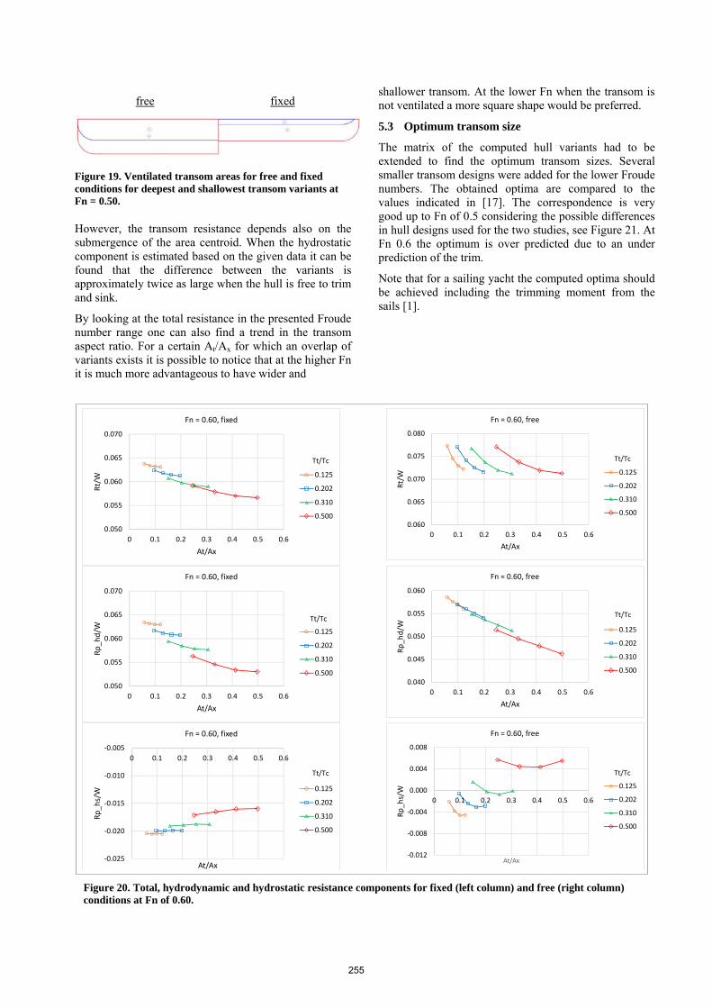
Figure 19. Ventilated transom areas for free and fixed conditions for deepest and shallowest transom variants at Fn = 0.50.

However, the transom resistance depends also on the submergence of the area centroid. When the hydrostatic component is estimated based on the given data it can be found that the difference between the variants is approximately twice as large when the hull is free to trim and sink.

By looking at the total resistance in the presented Froude number range one can also find a trend in the transom aspect ratio. For a certain At/Ax for which an overlap of variants exists it is possible to notice that at the higher Fn it is much more advantageous to have wider and

shallower transom. At the lower Fn when the transom is not ventilated a more square shape would be preferred.

5.3 Optimum transom size

The matrix of the computed hull variants had to be extended to find the optimum transom sizes. Several smaller transom designs were added for the lower Froude numbers. The obtained optima are compared to the values indicated in [17]. The correspondence is very good up to Fn of 0.5 considering the possible differences in hull designs used for the two studies, see Figure 21. At Fn 0.6 the optimum is over predicted due to an under prediction of the trim.

Note that for a sailing yacht the computed optima should be achieved including the trimming moment from the sails [1].

Figure 20. Total, hydrodynamic and hydrostatic resistance components for fixed (left column) and free (right column) conditions at Fn of 0.60.

free fixed

255

0

0.05

0.1

0.15

0.2

0.25

0.3

0.35

0.4

0.3 0.35 0.4 0.45 0.5 0.55 0.6 0.65

At/Ax 

Fn

CFD

PNA

Figure 21. Best At/Ax from the calculations (blue) compared to optima from Principles of Naval Architecture (red)

6. CONCLUSIONS

For the wet transom its area should be as small as possible within the extended size range that was indicated in Section 5.3. Both hydrodynamic and hydrostatic pressure resistance components have their minima for narrow and shallow transoms.

When the transom is ventilated the optimum size depends on the balance between the hydrostatic and hydrodynamic force components. The hydrostatic transom resistance increases with the transom size. However, it is constant with speed. On the other hand the hydrodynamic resistance decreases when the buttock and waterline curvature is reduced which can be achieved by increasing the transom size. Since the hydrodynamic component increases with speed squared it balances out the negative effect of the hydrostatic transom resistance at certain point, thus the optimum size can be found at each Froude number.

The transom width has much larger effect on resistance and trim than the draught. Both hydrostatic properties of the hull and flow pattern improve with wider transom at higher speeds. The lower waterline curvatures of the aft body additionally reduce wave generation downstream of maximum waterline beam.

Acknowledgements The authors would like to thank the Department of Shipping and Marine Technology at Chalmers University of Technology for providing necessary computational resources to perform the work.

References 1. Allroth, J. and Wu, T.-H. (2013), “A CFD

Investigation of Sailing Yacht Transom Sterns”, MSc Thesis, Dept. Shipping and Marine Technology, Chalmers University of Technology, Gothenburg, Sweden

2. Allroth, J., Wu, T.-H., Orych, M., Larsson, L. (2015), “Sailing Yacht Transom Sterns – A

Systematic CFD Investigation”, 5th High Performance Yacht Design, Auckland, New Zealand

3. Doctors, L., J., Macfarlane, G., J., Young, R., (2007) “A Study of Transom-Stern Ventilation”, International Shipbuilding Progress, Volume 54, Number 2-3 / 2007, pages 145-163

4. Toby, S., A., (2002) “To the Edge of the Possible: U.S. High Speed Destroyers, 1919–1942 Part 2: Secondary Hull Form Parameters”, Naval Engineers Journal, Volume 114, Issue 4, pages 55–76, October 2002

5. Broberg, L., Regnström, B., Östberg, M. (2007) “XCHAP – Theoretical Manual”, FLOWTECH International AB.

6. Menter, F.R. (1993) “Zonal Two Equation k-w Turbulence Models for Aerodynamic Flows”, 24th Fluid Dynamics Conference, Orlando, AIAA paper-93-2906.

7. Roe, P. L. (1981) “Approximate Riemann Solvers, Parameter Vectors, and Difference Schemes”, Journal of Computational Physics, Vol. 43, 357

8. Dick, E., Linden, J. (1992) “A Multigrid Method for Steady Incompressible Navier-Stokes Equations Based on Flux Difference Splitting”, International Journal for Numerical Methods in Fluids, Vol.14, 1311-1323

9. Chakravarthy, S. & Osher, S. (1985) “A New Class of High Accuracy TVD Schemes for Hyperbolic Conservation Laws”, AIAA paper-85-0363 .

10. Darwish, M., Moukalled, F. (2006) “Convective Schemes for Capturing Interfaces of Free-Surface Flows on Unstructured Grids”, Numerical Heat Transfer, Part B, 49: 19–42

11. Leonard, B. P. (1991) “The ULTIMATE conservative difference scheme applied to unsteady one-dimensional advection” Computer Methods in Applied Mechanics and Engineering, 88, 17-74.

12. Leveque, R. J. (1998) “Balancing Source Terms and Flux Gradients in High-Resolution Godunov Methods: The Quasi-Steady Wave-Propagation Algorithm” Journal of Computational Physics, 146, 346-365.

13. Hubbard, M. E., Garcia-Navarro, P. (2000) “Flux Difference Splitting and the Balancing of Source Terms and Flux Gradients” Journal of Computational Physics, Vol. 165(1), pp. 89-125

14. Orych, M., (2013) “Development of a Free Surface Capability in a RANS Solver with Coupled Equations and Overset Grids”, Lic. Eng. Thesis, Dept. Shipping and Marine Technology, Chalmers University of Technology, Gothenburg, Sweden

15. Eslamdoost, A., Larsson, L. and Bensow, R., (2014) “A pressure jump method for modeling waterjet/hull interaction”, Ocean Engineering (0029-8018). Vol. 88 (2014), p. 120–130.

16. Eslamdoost, A., Larsson, L. and Bensow, R., (2015) “On Transom Clearance”, Submitted to Ocean Engineering

17. Larsson, L. and Raven, H., (2010), “Ship Resistance and Flow”, PNA Series, SNAME, USA

256