Hydro-meteorological hazards assessment: practices in … · Gumbel 1960, Statistics of extremes Miquel (EDF) 1984, Guide d’estimation des débits de crue ... La Rochelle (Xynthia)

Claire-Marie DulucIRSN/SCAN/BEHRIG

Hydro-meteorological hazards assessment: practices in nuclear safety field and

scientific challenges

Symposium on Uncertainty Quantification in Computational Geosciences

january 15-17, 2018

http://www.brgm.eu/

Symposium on Uncertainty Quantification in Computational Geosciences – january 15-17, 2018

▌ IRSN: National expert for research and technical support on nuclear safety risk

▌ Site and Natural Hazards Department (SCAN)

▌ Hydrogeological, geotechnical, meteorological and flood hazards assessment section (BEHRIG)

Technical support to the French nuclear safety authority (ASN)

Research on meteorological and flood hazards

IRSN, Public assessment

Researchinto risks

Stakeholders (CLIs)

THE PUBLIC

Operator

Designers and constructors

Public authorities

Parliament

ASN, ASND

2


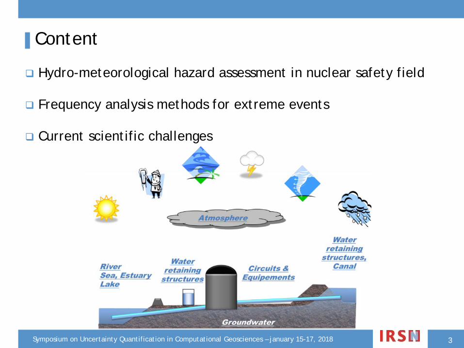
▌Content

Hydro-meteorological hazard assessment in nuclear safety field

Frequency analysis methods for extreme events

Current scientific challenges

3


▌General approach for external hazards

Event usually defined by 3 typical parameters Intensity Duration Frequency

Main steps : Characterization of an extreme hazard/event Hazard characterization at location(s) of interest Effects on structures/equipments

I. Hydro-meteorological hazard assessment in nuclear safety field

A very low target value of frequency“A common target value of frequency, not higherthan 10–4 per annum, shall be used for each designbasis event.” according to Safety reference level forexisting reactors (Wenra report, 2014)

4


International Atomic Energy Agency

Statement from the IAEA safety guides (IAEA Safety Standards - Specific Safety Guide No. SSG-18):

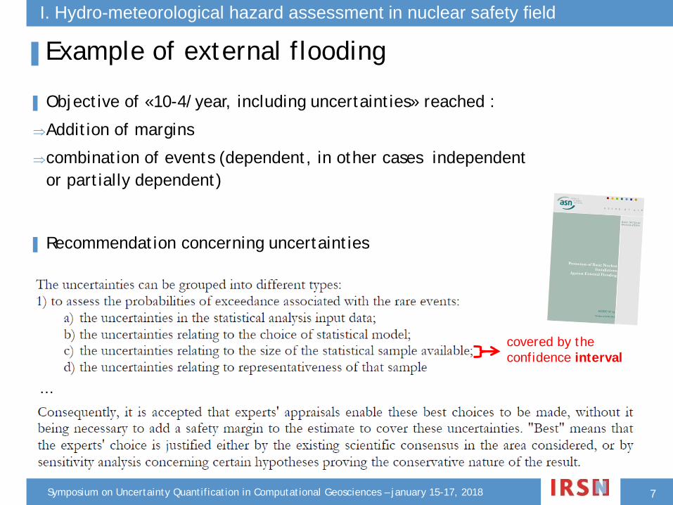
«The assessment of the hazards implies the need for treatment of the uncertainties in the process… »

▌Uncertainties …I. Hydro-meteorological hazard assessment in nuclear safety field

5


▌Reference Flood Situations (RFS) defined in the flooding guide (2013)

Deterministic approach with statistics of extremes used in several situations

▌Exemple of external floodingI. Hydro-meteorological hazard assessment in nuclear safety field

6

The target value frequency : «10-4/year » is lower than the state of art available with statistics of extremes (excepted for small watershed flooding)


▌Example of external flooding

covered by the confidence interval

7

…

▌ Objective of «10-4/year, including uncertainties» reached :

⇒Addition of margins

⇒combination of events (dependent, in other cases independent or partially dependent)

▌ Recommendation concerning uncertainties



▌Fields of application for statistics of extremes

Flood hazards :RainfallRiver flowSea surgesLocal wind waves (statistics on wind speed)Ocean waves

Extreme temperatures (max and min)

Extreme winds

Extreme snows


8


▌Frequency Analysis (FA) for extreme events

Non exceedance probability0 0.5 1

0

2

4

6

8

Empirical probabilities

Mag

nitu

de

0

2

4

6

1980 1995 2010 years

Data sample

p=0,999T=1000 years

1000 years Return level estimation

II. Frequency analysis methods

Mains stepsRaw data & Hypothesis testingFrequency model selectionDistribution selection and fittingAdequacy criterion & testsUncertainty estimationExtrapolation

9

Gumbel 1960, Statistics of extremes

Miquel (EDF) 1984, Guide d’estimationdes débits de crue

Coles 2001…


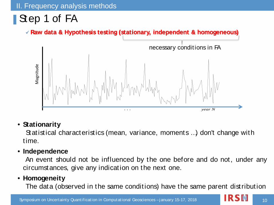
Raw data & Hypothesis testing (stationary, independent & homogeneous)

election;

Empirical probability compute;

A distribution selection and fitting (theoretical probabilities)

Adequacy criterion & tests;

Uncertainty estimation (confidence intervals);

Extrapolation (1000-year return level for example).. . . year N

Mag

nitu

de

• StationarityStatistical characteristics (mean, variance, moments …) don't change with

time.• Independence

An event should not be influenced by the one before and do not, under anycircumstances, give any indication on the next one.

• HomogeneityThe data (observed in the same conditions) have the same parent distribution

necessary conditions in FA

▌Step 1 of FAII. Frequency analysis methods

10



A frequency model selection

Empirical probability compute;

A distribution selection and fitting (theoretical probabilities)

Adequacy criterion & tests;

Uncertainty estimation (confidence intervals);

Extrapolation (1000-year return level for example).

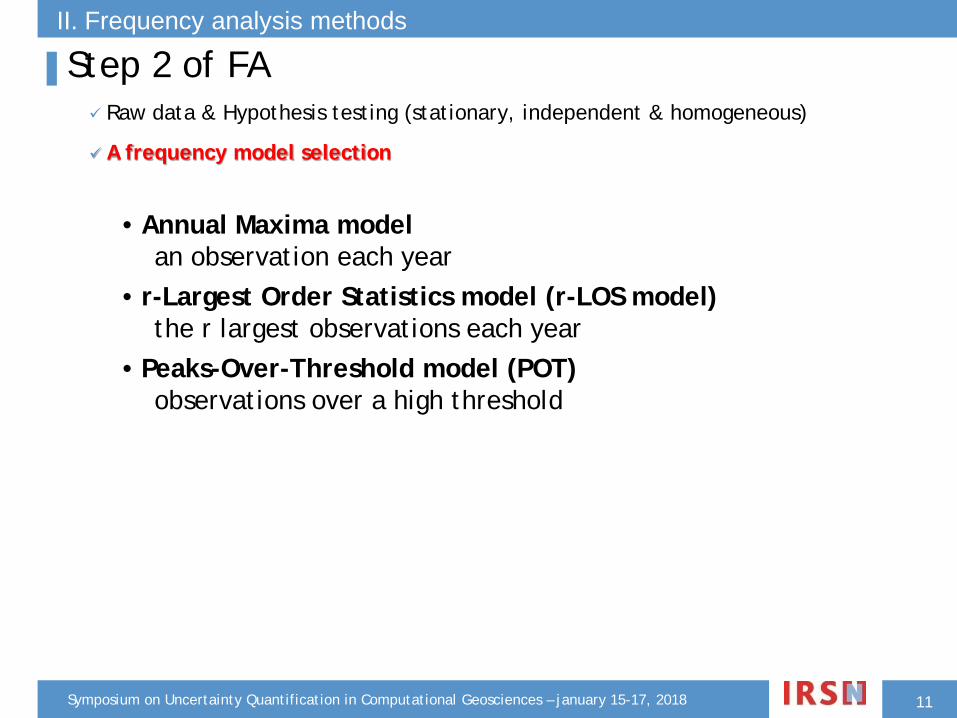
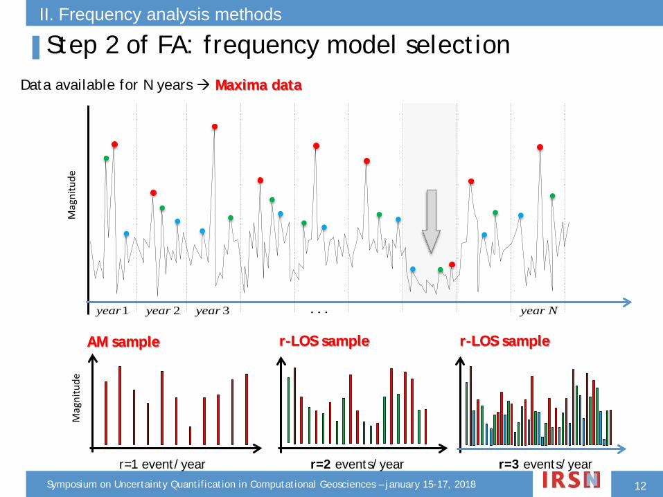
• Annual Maxima modelan observation each year

• r-Largest Order Statistics model (r-LOS model)the r largest observations each year

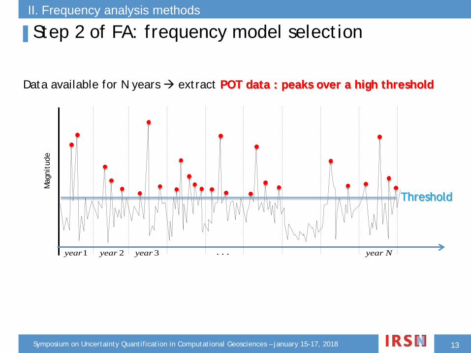
• Peaks-Over-Threshold model (POT) observations over a high threshold


11


1year . . .2year 3year year N

Mag

nitu

deData available for N years Maxima data

r-LOS sample r-LOS sample

Mag

nitu

de

r=1 event/year

AM sample

r=2 events/year r=3 events/year

▌Step 2 of FA: frequency model selectionII. Frequency analysis methods

12


1year . . .2year 3year year N

Mag

nitu

de

Threshold

Data available for N years extract POT data : peaks over a high threshold


13


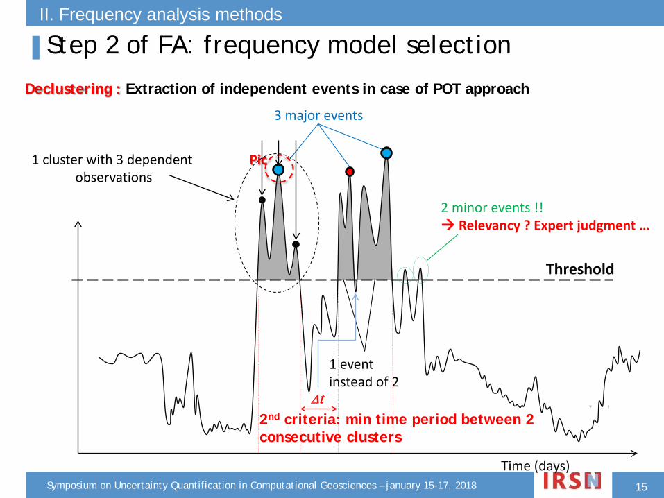
Declustering : Extraction of independent events in case of POT approach

Threshold

Time (days)


How many independent peaks in this case ?

14


Declustering : Extraction of independent events in case of POT approach

Threshold

Time (days)

1 eventinstead of 2

∆t2nd criteria: min time period between 2 consecutive clusters

2 minor events !! Relevancy ? Expert judgment …

3 major events

Pic1 cluster with 3 dependentobservations


15



Frequency model selection

Distribution selection and fitting (theoretical probabilities)

( ) ( )( )

1

1 : location parameter0/ , , : scale parameter

: shape parameter0x

x

e

er LOS GEV F xe

ξ

µ σ

µξσ

µξµ σ ξ σ

ξξ

−

− −

− − +

−

≠− ← = =

( ) ( ) ( )1

1 1 0

1 0/ , ,

xu

xG x

ePOT GPD

σ

ξ

µ

ξ ξσ

ξµ σ ξ

−=

− − ≠=

− =

←

▌Step 3 of FA

• Distribution of r-LOS extremes converges to a GEV ;

• Distribution of POT extremes converges to a GP ;

• Other distributions

(weibull, log normal, etc.)


16




Distribution selection and fitting

Adequacy criteria & tests

• Pearson test (Chi-2)• Kolmogorov-Smirnov test• …

Numerical check

( )22 ; 1i i

value pk i

np k n

νχ

ν−

= = − −∑

Chi2 : Check if a given sample comes from apriori distribution. This test focuses on thetheoretical and experimental numbers per class.

Kolmogorov-Smirnov: Same principle asChi2. But this test is interested in maxdistance between the observed andtheoretical distributions

( ) ( )sup nD F x F x= −

Visual check

2

4

6

8

2 4 6 8 computed

obse

rved

Q-Q plot


0 2 4 6 8


17




Distribution selection and fitting (theoretical probabilities)

Adequacy criteria & tests

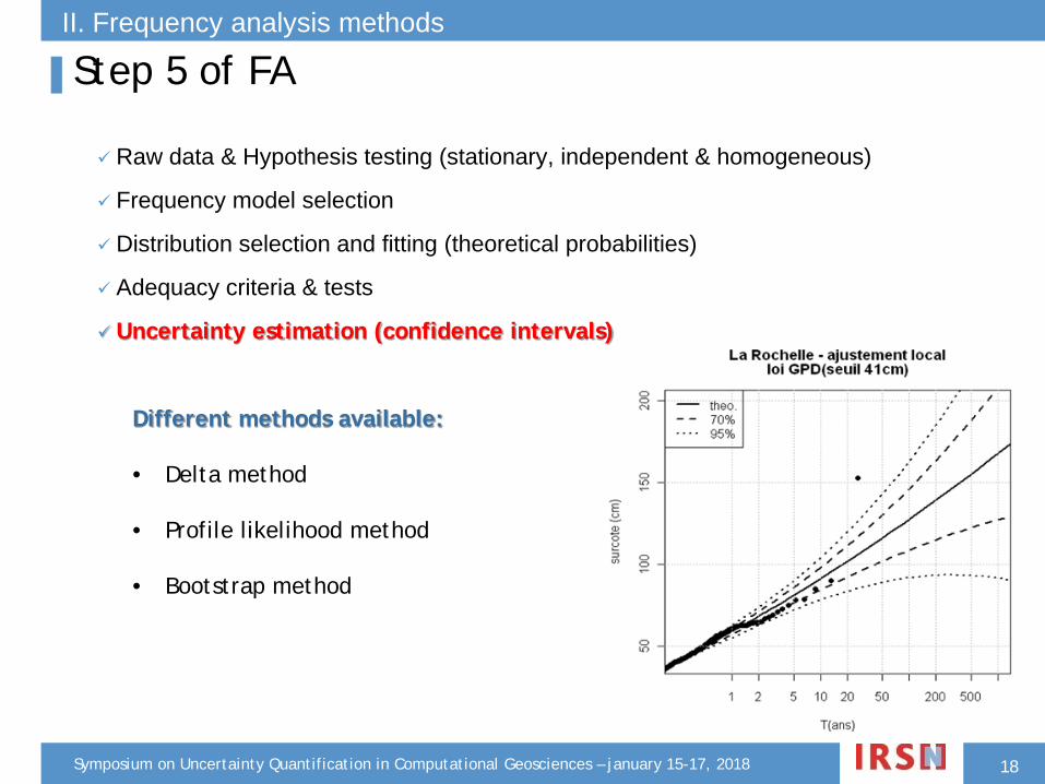
Uncertainty estimation (confidence intervals)

▌Step 5 of FA

Different methods available:

• Delta method

• Profile likelihood method

• Bootstrap method


18


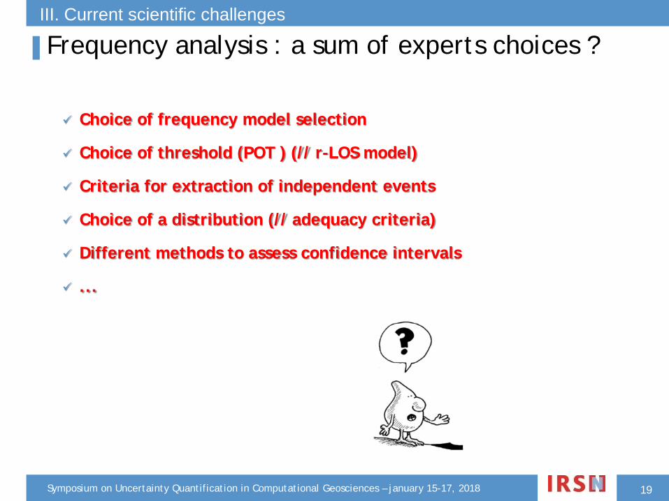
Choice of frequency model selection

Choice of threshold (POT ) (// r-LOS model)

Criteria for extraction of independent events

Choice of a distribution (// adequacy criteria)

Different methods to assess confidence intervals

...

▌Frequency analysis : a sum of experts choices ?III. Current scientific challenges

19


Logic tree combining various experts’ opinions & explore uncertainties on

parameters (PSHA framework)

▌Scientific challenge n°1 How to integrate knowledge / opinion of different experts ?

Roles and Interactions between experts in a SSHAC Level 3

⇒ Feedback: some relevant aspects to keep, simplification needed…

III. Current scientific challenges

20

⇒ SSHAC (Senior Seismic Hazard Analysis Committee) : a complete andrigorous method defined in the framework of PSHA (Probabilistic SeismicHazard Analysis)


Mag

nitu

de

0

2

4

6

8

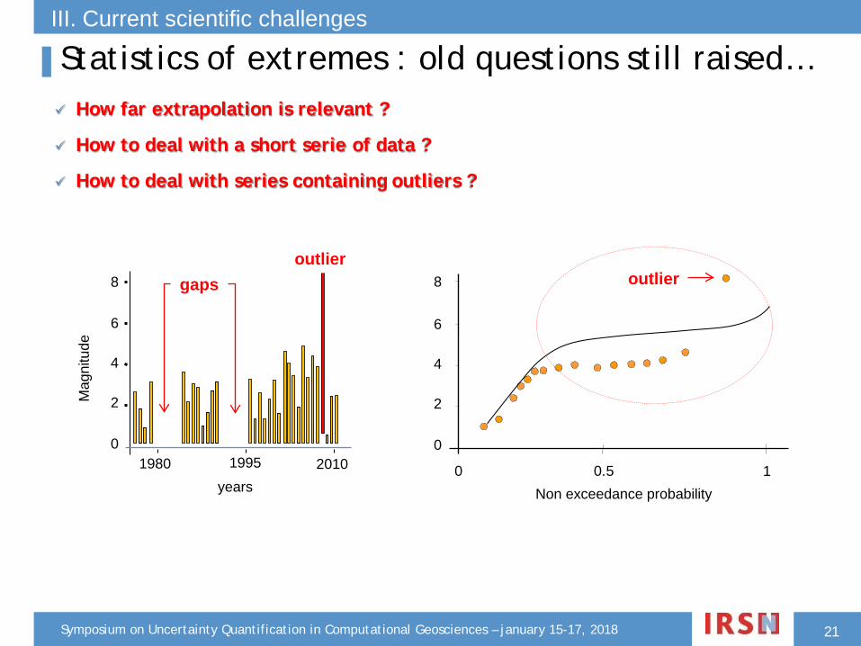
1980 1995 2010 years

gaps


0

2

4

6

8 outlier

outlier

▌Statistics of extremes : old questions still raised… How far extrapolation is relevant ?

How to deal with a short serie of data ?

How to deal with series containing outliers ?


21


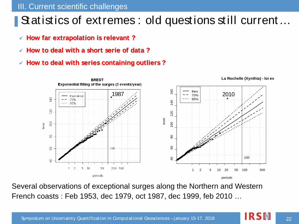
1987

4060

8010

012

014

016

0

La Rochelle (Xynthia) - loi ex

periods

leve

l

1 2 5 10 20 50 100 500

theo.70%95%

100

2010

Several observations of exceptional surges along the Northern and Western French coasts : Feb 1953, dec 1979, oct 1987, dec 1999, feb 2010 …


▌Statistics of extremes : old questions still current…

22

How far extrapolation is relevant ?

How to deal with a short serie of data ?

How to deal with series containing outliers ?


Météo-France (local data 2010)http://climatheque.meteo.fr

Programme « Renext » de l’IRSN https://gforge.irsn.fr/gf/project/renext/

⇒ Strong impact of a single value…

Rainfall


▌Outliers, an issue for various hazards…

23

http://climatheque.meteo.fr/

https://gforge.irsn.fr/gf/project/renext/


snow



24


snow

Try anyway ?...

• Log exp distribution ?• Change of variable ?



25


snow

Eurocode :

The approach is to not take into consideration outliers and complete the safety approach through a margin (accidental design)


26



Non exceedance probability0 1

outlier

surg

es



Integration of additional information

the Netherlands, 17e century

Historical information

Regional information

27



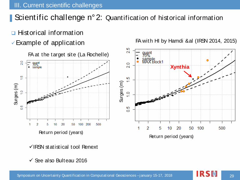
▌Scientific challenge n°2: Quantification of historical information

Historical informationMiquel 1984, Hosking &Wallis 1987, Coles 2001, Payrastre 2005, Neppel

2010…Methods and operational tools are available (with both frequentist or

Bayesian methods)

Known value

Lower Bound Range

Threshold of perception

years

Surg

es(c

m)

0

50

100

150

200

1800 2000 1700 1900

Syst. periodHistorical period

28




Historical informationExample of application

IRSN statistical tool Renext

See also Bulteau 2016

29

FA with HI by Hamdi &al (IRSN 2014, 2015)

Xynthia

Surg

es (

m)

Return period (years)

FA at the target site (La Rochelle)

Surg

es (

m)

Return period (years)



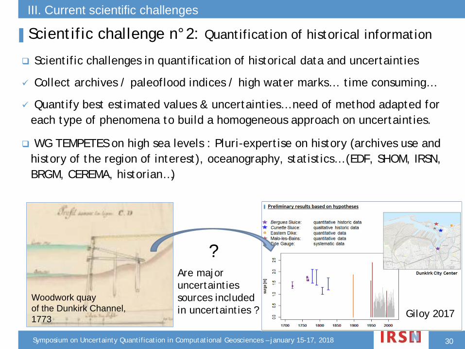
Scientific challenges in quantification of historical data and uncertainties

Collect archives / paleoflood indices / high water marks… time consuming…

Quantify best estimated values & uncertainties… need of method adapted for each type of phenomena to build a homogeneous approach on uncertainties.

WG TEMPETES on high sea levels : Pluri-expertise on history (archives use and history of the region of interest), oceanography, statistics… (EDF, SHOM, IRSN, BRGM, CEREMA, historian…)

Woodwork quay of the Dunkirk Channel,1773


?

Giloy 2017

30

Are major uncertainties sources included in uncertainties ?



Regional information Hosking et Wallis (1997)

Use for river flow (gauged vs ungauged sites) for many years

Important work concerning rainfalls, and more recently sea surges …

Principle : Merging data from a homogeneous region in a common dataset

Local effects taken through a local index

Key question of the spatial & temporal dependency between data

Concept of “equivalent station years” or “regional effective duration” to characterize the dependency between data at different locations of the homogeneous region

Regional approach more and more broadly used Results from regional approaches now published by Meteo-France for rainfall :

Shyreg, local-regional distribution, local distr.(GEV)

31

▌Scientific challenge n°3: practice & upgrade regional approaches


Typical storms footprints used in a spatiotemporal declustering procedure(J. Weiss thesis 2014)

Use of the spatial extremogram to form a homogeneous region centrered on a target site for the regional frequency analysis (Hamdi 2016)

Recent work on extreme storm surgesin the nuclear safety field

EDF: J. Weiss PhD in 2014 Regional frequency analysis of extreme marine hazards + on going doctoral thesis by R. Frau

IRSN: Bardet 2011, Hamdi 2016

On going research to combine historical and regional information Still a lot to do to adapt/upgrade regional methods coming from river flow and rainfall to other natural hazards

32


▌Scientific challenge n°3: practice & upgrade regional approaches


What can we learn from past events in a context of climate change ?

What is the importance of this “new” epistemic uncertainty compared to otheruncertainties ?


▌Non stationarity & Climate change

33



Methods and operational tools available in nuclear safety field

EDF : publications by Parey & LSCE

IRSN : NSGEV tool developed to test various hypothesis of non stationarity

Time-varying GEV distribution In practice : up to quadratic dependence on time for μ and σ Model the time series with multiple linear trends and locate the times of

significant changes (Break dates) Use of AIC, BIC and likelihood ratio to select the best time-varying model Calculation of the CI: delta, profile likelihood and bootstrap but does not

include uncertainty on the choice of time varying model…

Adaptation of the classic definition of the return period

Return period conditional to a fixed date Return period integrated over a future period: RL corresponds to an

expected number of exceedances equal to 1 over this period (Parey 2007)

▌Scientific challenge n°4: uncertainties due to climate change

34


Maximize likelihood to identify a breaking point

▌Scientific challenge n°5: uncertainties due to climate change

Choice of a time varying model…


35



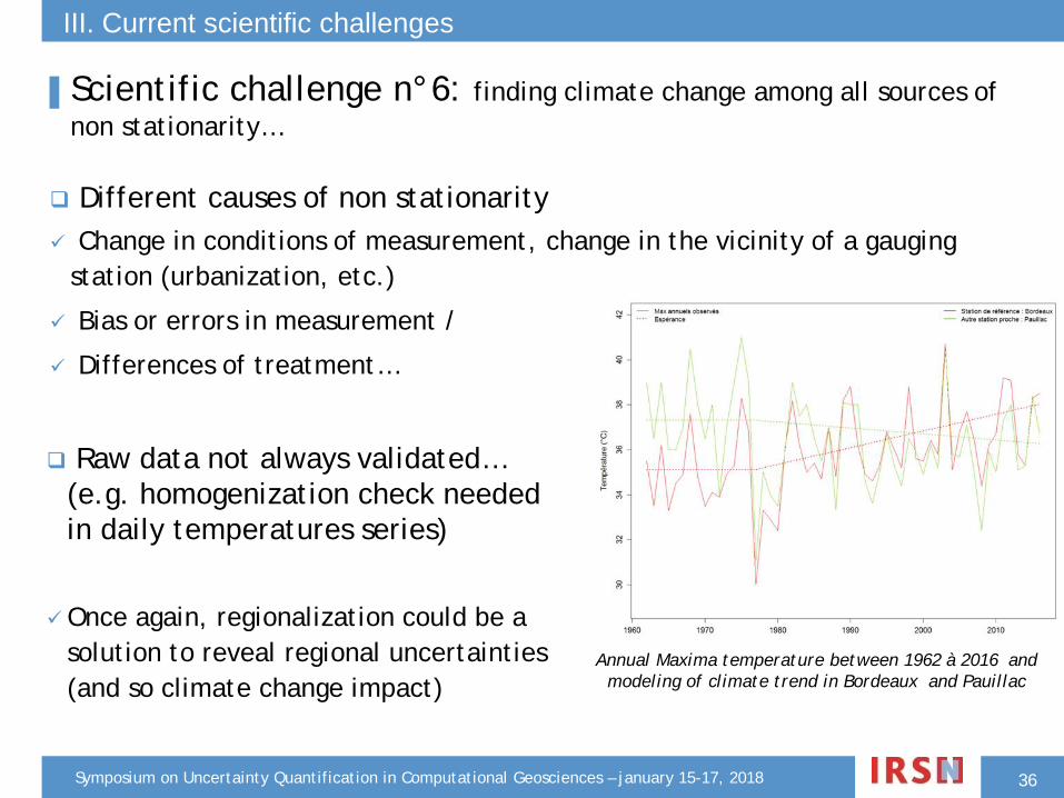
Different causes of non stationarity Change in conditions of measurement, change in the vicinity of a gauging

station (urbanization, etc.)

Bias or errors in measurement /

Differences of treatment…

Annual Maxima temperature between 1962 à 2016 and modeling of climate trend in Bordeaux and Pauillac

▌Scientific challenge n°6: finding climate change among all sources of non stationarity…

Raw data not always validated… (e.g. homogenization check needed in daily temperatures series)

Once again, regionalization could be a solution to reveal regional uncertainties (and so climate change impact)

36


▌Combining hazards..

Dependent / independent events… ?

Dealing with “correlated hazards”, “coexistent hazards”, “combined effects”, “associated effects” …

Multivariate statistical approach

Joint Probability method

Variable A

Variable B

?

A challenge is the characterization of dependency between extremes hazards (lack of observations and expertise)


37

Combining hazards (dependent an independent) & build a complete probabilistic approach, including uncertainty propagation (e.g. Probabilistic Flood Hazard Assessment)


▌Conclusion – challenges in research and practices

Work on data collect additional information (historical, regional) and quantify uncertainties

Consolidate homogeneous series (especially when time-varying models are used)

Identify and assess impact of climate change uncertainties among all sources of uncertainties…

Develop, adapt and spread the practice of statistics models dealing with both historic information (sometimes imprecise) and regional information (in particular Bayesian approaches)

Investigate methods to combine hazards (dependent and independent) and build a complete probabilistic approach, including uncertainty propagation (e.g. Probabilist Flood Hazard Assesment)

Define new approaches to better take into account the amount of knowledge (and sometimes of disagreements) coming from experts

38


Thank you


III. Reference Flood Situations (RFS)Probabilistic objective: 10-4 / year, with uncertainties

RFS Basis Hazard Increase / combination of events

PLU: Local rainfall 100-yr rainfall events (taking the Upper Bound – UB – of the 95% Confidence Interval – CI)

Surface water runoff situation + local stormwater drainage system completely blocked

CPB: Small watershledflooding

10,000 yrs instantaneous peak flow floodOR (10 < watershed < 100 km² only)

100-yr rainfalls event (UB of the 95% CI) + multiplying the resulting flow by a factor of 2

CGB: Large watershed flooding

1,000-yr flood (UB of the 70% CI) + influencing parameter + 15%

DDOCE: Malfunctioning of structures, circuits or

equipment

Deterministic simple failure or multiple common failures according to the scenario (earthquake…)

INT: Mechanically induced wave

Deterministic approach according to the initiator event

+ worst-case water level scenario

RNP: High groundwater level

Rise effect caused by an initiating event Initial level: 10-yr flood

Or

100-yr Groundwater level (UB of the 95% CI) Penalising hydrogeological hypotheses

ROR: Failure of a water-retaining structure

Deterministic failure of the dam +15 % + influencing parameter

CLA: Local wind waves 100-yr chop (UB of the 70% CI) Propagated over the 1,000-yr flood (UB of the 70% CI)

NMA: Sea level maximum level of the theoretical tide+ expectable climatic evolution

1,000-yr storm surge

(UB of the 70% CI)

+ 1 meter (to take account the “outliers”)

Or statistic model for “outliers” (extreme event)

VAG: Ocean waves 100 yrs wave swell (UB of the 70% CI) Propagated over the reference sea level (NMA)

SEI: Seiche Height of annual seiche Propagated over the reference sea level (NMA)

Documents

Hydro-meteorological hazards assessment: practices in … · Gumbel 1960, Statistics of extremes Miquel (EDF) 1984, Guide d’estimation des débits de crue ... La Rochelle (Xynthia)