Hydraulics and mixing in the Hudson River estuary: A numerical

model study of tidal variations during neap tide conditions

Petter StenstromDepartment of Land and Water Resources Engineering, Royal Institute of Technology, Stockholm, Sweden

Received 19 May 2003; revised 16 February 2004; accepted 27 February 2004; published 21 April 2004.

[1] Three-dimensional numerical modeling is performed to study intratidal and along-channel variability in stratification and mixing in the Hudson River estuary. The modeledfields show good agreement with observations, both qualitatively and quantitatively.Estuarine circulation dominates the mean fields, and intratidal variability is dominated bytidal straining that acts to strengthen the stratification during ebb and weaken it duringflood. Mixing is mainly confined to a bottom layer during flood but occurs higher up inthe water column during ebb. Mixing across the halocline shows marked along-channelvariability due to bathymetric effects. During ebb, mixing occurs preferentially at anabrupt channel expansion seaward of a channel constriction at the George WashingtonBridge, as predicted by Chant and Wilson [2000]. The salt flux across the halocline in thisregion, averaged over ebb, exceeds 5 � 10�4 kg m�2 s�1, a factor of 3 greater than thealong-channel average. Increased residence time of tracers should be expected in thisregion due to the strong mixing but also due to observed secondary circulation [Chant andWilson, 1997]. Mixing across the halocline during flood is small, except for earlyflood, before the well-mixed bottom layer is developed. Mixing is then localized to thelandward slope of sills. INDEX TERMS: 4235 Oceanography: General: Estuarine processes; 4255

Oceanography: General: Numerical modeling; 4568 Oceanography: Physical: Turbulence, diffusion, and

mixing processes; KEYWORDS: estuarine circulation, stratification, turbulent mixing, salt flux, tide, numerical

modeling

Citation: Stenstrom, P. (2004), Hydraulics and mixing in the Hudson River estuary: A numerical model study of tidal variations

during neap tide conditions, J. Geophys. Res., 109, C04019, doi:10.1029/2003JC001954.

1. Introduction

[2] The temporal variation of the stratification in estuariesreflects the competition between mean advective processesthat act to increase the stratification and stabilize the watercolumn, and turbulent mixing that acts in the oppositedirection. The mean advection, the so-called estuarinecirculation, is due to the longitudinal density gradient thatis the main characteristic of an estuary, with lighter water atthe head and denser water seaward. This longitudinaldensity gradient, together with the surface setup at the headdue to the freshwater discharge, drives a circulation wherelighter water is carried seaward on top of a return current ofheavier seawater. Tidal forcing interacts with this circulationin various ways. During ebb when the tidal wave withdrawsseaward, the bed shear acts together with the estuarinecirculation to promote stratification; with weak mixing,maximum stratification is reached near low water. Con-versely, during flood, the bed shear counteracts the estuarinecirculation to reduce stratification, which reaches a mini-mum near high water. This process is known as tidalstraining of the density field [Simpson et al., 1990]. Thetide also supplies mixing energy so that topography-inducedturbulence (tidal stirring), shear instabilities and breaking

internal waves all contribute to vertical exchange of mo-mentum and tracers. Further, Nepf and Geyer [1996] usedthe term overstraining to denote conditions at the end offlood under which tidal straining may overturn parts of thedensity field, producing regions of hydrostatic instabilityand subsequent convective mixing.[3] The interaction between the estuarine circulation and

turbulent mixing is nonlinear in the sense that the stablestratification produced by the advection of lighter fluid overheavier in the estuarine circulation inhibits turbulent mix-ing, while at the same time turbulent mixing diffuses themomentum of the estuarine circulation vertically, therebyreducing the horizontal advection. Owing to this feedback,small changes in the turbulent mixing energy supplied bythe tide or other sources may lead to large changes in thecirculation [Jay and Smith, 1990]. Particularly when thevelocities associated with the river discharge, tidal velocitiesand density-driven shear velocities are all of the samemagnitude, a strong interaction and a strong variability overa tidal cycle should be expected.[4] From an ecological perspective, the balance between

advective and turbulent processes is important because theestuarine circulation is the most efficient mechanism forflushing river-borne pollutants out to the open sea; thegreatest horizontal mass flux occurs at maximum stratifica-tion and minimum turbulent mixing [Nunes Vaz et al.,1989]. Turbulent mixing increases the tracer residence time

JOURNAL OF GEOPHYSICAL RESEARCH, VOL. 109, C04019, doi:10.1029/2003JC001954, 2004

Copyright 2004 by the American Geophysical Union.0148-0227/04/2003JC001954$09.00

C04019 1 of 12

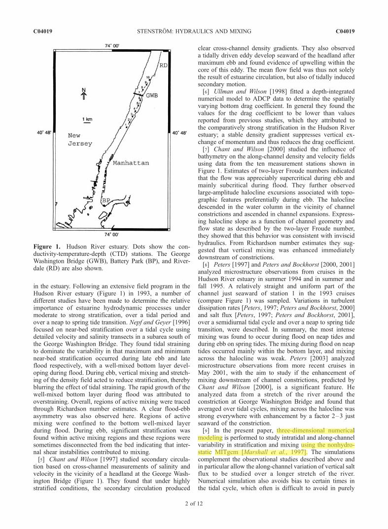
in the estuary. Following an extensive field program in theHudson River estuary (Figure 1) in 1993, a number ofdifferent studies have been made to determine the relativeimportance of estuarine hydrodynamic processes undermoderate to strong stratification, over a tidal period andover a neap to spring tide transition. Nepf and Geyer [1996]focused on near-bed stratification over a tidal cycle usingdetailed velocity and salinity transects in a subarea south ofthe George Washington Bridge. They found tidal strainingto dominate the variability in that maximum and minimumnear-bed stratification occurred during late ebb and lateflood respectively, with a well-mixed bottom layer devel-oping during flood. During ebb, vertical mixing and stretch-ing of the density field acted to reduce stratification, therebyblurring the effect of tidal straining. The rapid growth of thewell-mixed bottom layer during flood was attributed tooverstraining. Overall, regions of active mixing were tracedthrough Richardson number estimates. A clear flood-ebbasymmetry was also observed here. Regions of activemixing were confined to the bottom well-mixed layerduring flood. During ebb, significant stratification wasfound within active mixing regions and these regions weresometimes disconnected from the bed indicating that inter-nal shear instabilities contributed to mixing.[5] Chant and Wilson [1997] studied secondary circula-

tion based on cross-channel measurements of salinity andvelocity in the vicinity of a headland at the George Wash-ington Bridge (Figure 1). They found that under highlystratified conditions, the secondary circulation produced

clear cross-channel density gradients. They also observeda tidally driven eddy develop seaward of the headland aftermaximum ebb and found evidence of upwelling within thecore of this eddy. The mean flow field was thus not solelythe result of estuarine circulation, but also of tidally inducedsecondary motion.[6] Ullman and Wilson [1998] fitted a depth-integrated

numerical model to ADCP data to determine the spatiallyvarying bottom drag coefficient. In general they found thevalues for the drag coefficient to be lower than valuesreported from previous studies, which they attributed tothe comparatively strong stratification in the Hudson Riverestuary; a stable density gradient suppresses vertical ex-change of momentum and thus reduces the drag coefficient.[7] Chant and Wilson [2000] studied the influence of

bathymetry on the along-channel density and velocity fieldsusing data from the ten measurement stations shown inFigure 1. Estimates of two-layer Froude numbers indicatedthat the flow was appreciably supercritical during ebb andmainly subcritical during flood. They further observedlarge-amplitude halocline excursions associated with topo-graphic features preferentially during ebb. The haloclinedescended in the water column in the vicinity of channelconstrictions and ascended in channel expansions. Express-ing halocline slope as a function of channel geometry andflow state as described by the two-layer Froude number,they showed that this behavior was consistent with inviscidhydraulics. From Richardson number estimates they sug-gested that vertical mixing was enhanced immediatelydownstream of constrictions.[8] Peters [1997] and Peters and Bockhorst [2000, 2001]

analyzed microstructure observations from cruises in theHudson River estuary in summer 1994 and in summer andfall 1995. A relatively straight and uniform part of thechannel just seaward of station 1 in the 1993 cruises(compare Figure 1) was sampled. Variations in turbulentdissipation rates [Peters, 1997; Peters and Bockhorst, 2000]and salt flux [Peters, 1997; Peters and Bockhorst, 2001],over a semidiurnal tidal cycle and over a neap to spring tidetransition, were described. In summary, the most intensemixing was found to occur during flood on neap tides andduring ebb on spring tides. The mixing during flood on neaptides occurred mainly within the bottom layer, and mixingacross the halocline was weak. Peters [2003] analyzedmicrostructure observations from more recent cruises inMay 2001, with the aim to study if the enhancement ofmixing downstream of channel constrictions, predicted byChant and Wilson [2000], is a significant feature. Heanalyzed data from a stretch of the river around theconstriction at George Washington Bridge and found thataveraged over tidal cycles, mixing across the halocline wasstrong everywhere with enhancement by a factor 2–3 justseaward of the constriction.[9] In the present paper, three-dimensional numerical

modeling is performed to study intratidal and along-channelvariability in stratification and mixing using the nonhydro-static MITgcm [Marshall et al., 1997]. The simulationscomplement the observational studies described above andin particular allow the along-channel variation of vertical saltflux to be studied over a longer stretch of the river.Numerical simulation also avoids bias to certain times inthe tidal cycle, which often is difficult to avoid in purely

Figure 1. Hudson River estuary. Dots show the con-ductivity-temperature-depth (CTD) stations. The GeorgeWashington Bridge (GWB), Battery Park (BP), and River-dale (RD) are also shown.

C04019 STENSTROM: HYDRAULICS AND MIXING

2 of 12

C04019

observational studies. The results are compared to the overallbehavior described by Nepf and Geyer [1996] and Chant andWilson [2000]. Modeled vertical salt fluxes are compared tothe estimates of Nepf and Geyer [1996], Peters [1997, 2003],and Peters and Bockhorst [2001]. The forcing is chosento represent a semidiurnal tidal cycle during neap tideconditions. Results are presented for an 8 km stretch of theriverwith comparatively large changes in cross-sectional area.[10] Below, the measurements are first briefly described

in section 2, followed by a description of the numericalmodel and the numerical simulations in section 3. Insection 4, the modeled fields are analyzed with regard tohydraulics and mixing. The results are then discussed insection 5.

2. Data

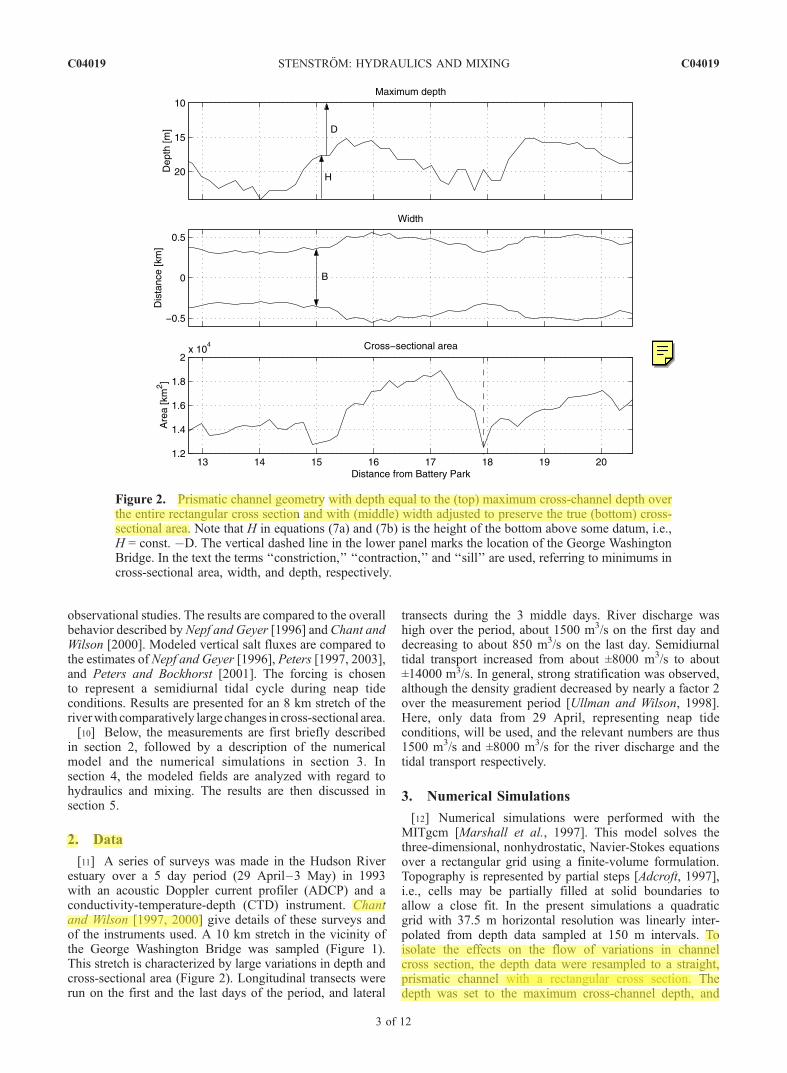
[11] A series of surveys was made in the Hudson Riverestuary over a 5 day period (29 April–3 May) in 1993with an acoustic Doppler current profiler (ADCP) and aconductivity-temperature-depth (CTD) instrument. Chantand Wilson [1997, 2000] give details of these surveys andof the instruments used. A 10 km stretch in the vicinity ofthe George Washington Bridge was sampled (Figure 1).This stretch is characterized by large variations in depth andcross-sectional area (Figure 2). Longitudinal transects wererun on the first and the last days of the period, and lateral

transects during the 3 middle days. River discharge washigh over the period, about 1500 m3/s on the first day anddecreasing to about 850 m3/s on the last day. Semidiurnaltidal transport increased from about ±8000 m3/s to about±14000 m3/s. In general, strong stratification was observed,although the density gradient decreased by nearly a factor 2over the measurement period [Ullman and Wilson, 1998].Here, only data from 29 April, representing neap tideconditions, will be used, and the relevant numbers are thus1500 m3/s and ±8000 m3/s for the river discharge and thetidal transport respectively.

3. Numerical Simulations

[12] Numerical simulations were performed with theMITgcm [Marshall et al., 1997]. This model solves thethree-dimensional, nonhydrostatic, Navier-Stokes equationsover a rectangular grid using a finite-volume formulation.Topography is represented by partial steps [Adcroft, 1997],i.e., cells may be partially filled at solid boundaries toallow a close fit. In the present simulations a quadraticgrid with 37.5 m horizontal resolution was linearly inter-polated from depth data sampled at 150 m intervals. Toisolate the effects on the flow of variations in channelcross section, the depth data were resampled to a straight,prismatic channel with a rectangular cross section. Thedepth was set to the maximum cross-channel depth, and

Figure 2. Prismatic channel geometry with depth equal to the (top) maximum cross-channel depth overthe entire rectangular cross section and with (middle) width adjusted to preserve the true (bottom) cross-sectional area. Note that H in equations (7a) and (7b) is the height of the bottom above some datum, i.e.,H = const. �D. The vertical dashed line in the lower panel marks the location of the George WashingtonBridge. In the text the terms ‘‘constriction,’’ ‘‘contraction,’’ and ‘‘sill’’ are used, referring to minimums incross-sectional area, width, and depth, respectively.

C04019 STENSTROM: HYDRAULICS AND MIXING

3 of 12

C04019

the width was adjusted to preserve the true cross-sectionalarea (Figure 2).

3.1. Subgrid Parameterization

[13] Given a flux-gradient form for turbulent correlations[e.g., Rodi, 1987] and further assuming that the time-dependent, advective and diffusive terms can be neglected[Peters and Bockhorst, 2001], the balance for turbulentkinetic energy can be written

e ¼ P þ B ¼ Km

@u

@z

� �2

þ @v

@z

� �2 !

þ Krg

r0

@r@z

; ð1Þ

that is, a steady local balance is assumed between shearproduction, P, buoyancy production, B, and viscousdissipation, e. The coefficients of eddy viscosity and eddydiffusivity are denoted Km and Kr. Following Smagorinsky[1963], the eddy viscosity coefficient is expressed as

Km ¼ CSDð Þ4=3e1=3; ð2Þ

where CS is a constant and D is the nominal grid spacing.Inserting equation (1) into equation (2) gives

Km ¼ CSDð Þ2ffiffiffiffiffiffiffiffiffiffiffiffiffiffiffiffiffiffiffiffiffiffiffiffiffiffiffiffiffiffiffiffiffiffiffiffiffiffiffiffiffiffiffiffiffiffiffiffiffiffiffiffiffiffi@u

@z

� �2

þ @v

@z

� �2

þ Kr

Km

g

r0

@r@z

s: ð3Þ

A scheme was implemented in the model that calculates the(vertical) eddy coefficients from equation (3) locally atevery time step. Following Winters and Seim [2000], Km =Kr was assumed, i.e., a turbulent Prandtl number of unity.When the square root argument in equation (3) is negative,Km and Kr are set to the background values 10�4 m2/s and10�6 m2/s respectively. The larger value for Km is neededfor numerical stability. The horizontal eddy coefficientswere held constant. The values for the Smagorinskyconstant, CS, and for the horizontal eddy coefficients aregiven in Table 1, together with other parameters for thesimulations. The vertical grid resolution was set to 0.2 m,which is in the lower part of the range of turbulentoverturning scales found during ebb by Peters [1997] andPeters and Bockhorst [2000]. During flood, the overturningscales are larger. Most of these overturning scales are thusexplicitly simulated.

3.2. Boundary Conditions

[14] At the upper boundary the model has an implicitfree surface formulation and at solid boundaries a no-slip

condition was used. At the lateral open boundaries (notethat these are located at Battery Park and Riverdale (com-pare Figure 1), i.e., far from the region of interest aroundGeorge Washington Bridge), a modification of the conditionproposed by Khatiwala [2003] was used. This is a two-partcondition that decomposes the total velocity at the boundaryinto a depth-independent (vertically averaged) part and aperturbation part and treats them separately. The perturba-tion velocity is radiated out of the domain using a variantof the Orlanski [1976] implementation of the classicalSommerfeld radiation condition. The depth-independentpart, U, is also radiated, using a simple integrated condition[cf. Nycander and Doos, 2003; Stenstrom, 2003]:

U � chD¼ 0; ð4Þ

where h is the sea level perturbation and D is depth. Thephase velocity was set to the speed of a long gravity wave,i.e., c = ±

ffiffiffiffiffiffigD

p, with the negative (positive) sign at the left

(right) boundary. To force a net flow through the domain, aforcing term was added to the right hand side of equation (4)at the seaward boundary:

FU ¼ UR þ U0 sin 2pt

T

� �; ð5Þ

where UR is the river discharge, U0 is the amplitude of thetidal wave, t is time, and T is the period.[15] Data were available neither for the seaward bound-

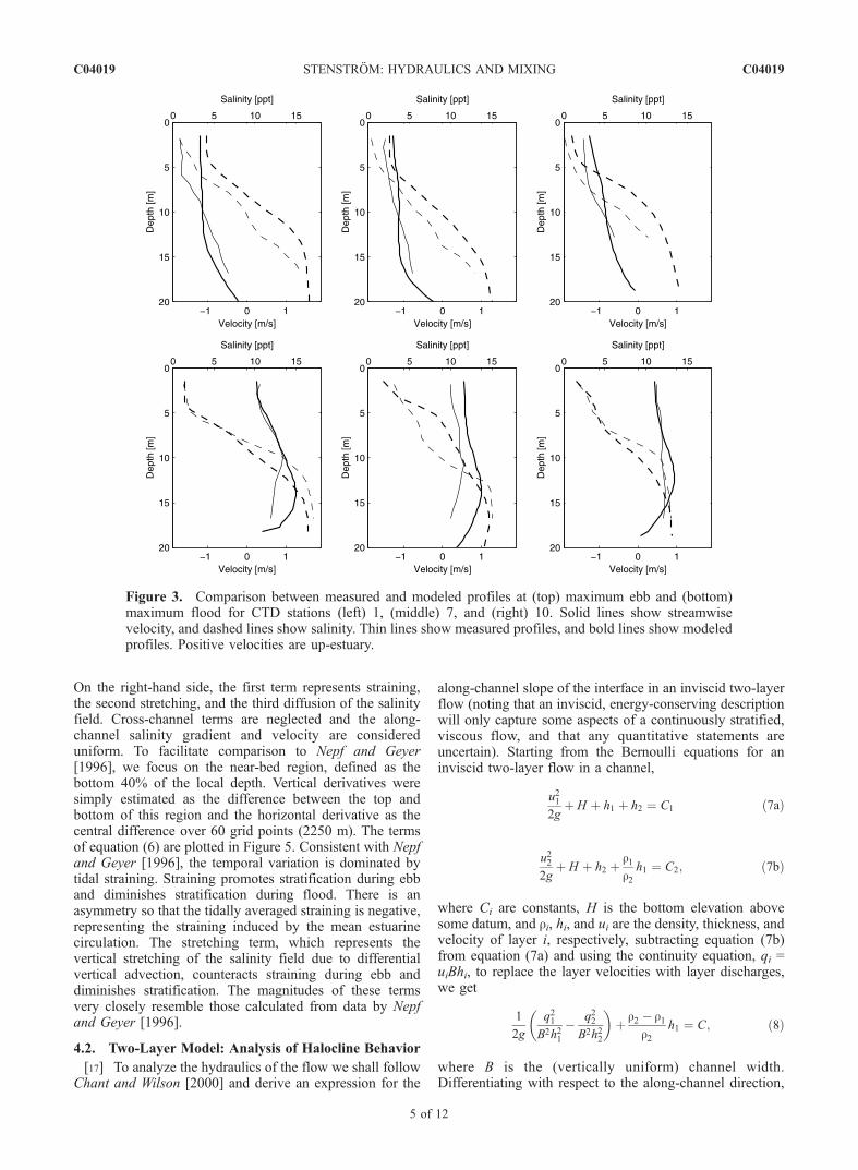
ary at Battery Park nor for the landward boundary atRiverdale. Instead a uniform time-dependent velocity wasforced at the seaward boundary, consistent with the mea-sured time-dependent net flow due the tide and the riverdischarge. Salinity profiles at the boundaries were adjustediteratively by simple trial and error to fit data at CTDstations in the interior. Figure 3 shows a comparisonbetween modeled and measured profiles at CTD stations1, 7 and 10, i.e., at the boundaries of the central reach thatwas in focus during the field program and at the headland atthe George Washington Bridge. While the fit could beimproved, this was not considered vital for the purpose ofthe present study; of most importance for an assessment ofthe dynamics is that the magnitude of the different flowcomponents, the river discharge and the barotropic tide, andthe salinity range agree well with the measured conditions.

4. Results

4.1. Temporal Variation in Stratification

[16] The modeled salinity field at four points over thetidal cycle is shown in Figure 4. Consistent with themeasurements, the stratification is nearly linear from max-imum ebb to late ebb. During flood a well-mixed bottomlayer propagates landward through the domain and lifts thesalinity field to create a sharper halocline above. For closerassessment of the temporal variation in stratification, theadvection-diffusion equation for salt is vertically differenti-ated, following Nepf and Geyer [1996]:

@

@t

@S

@z¼ � @u

@z

@S

@x� @w

@z

@S

@zþ @

@z

@

@zKr

@S

@z

� �: ð6Þ

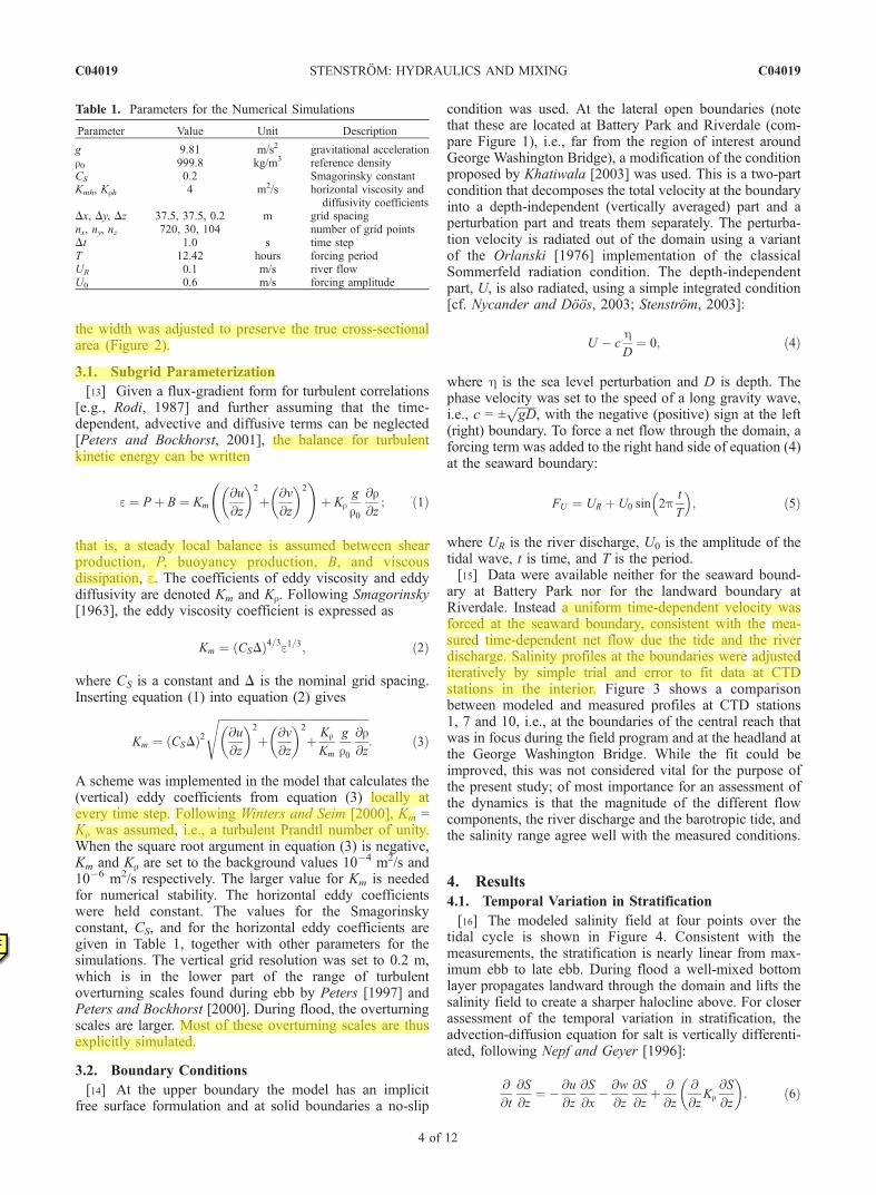
Table 1. Parameters for the Numerical Simulations

Parameter Value Unit Description

g 9.81 m/s2 gravitational accelerationr0 999.8 kg/m3 reference densityCS 0.2 Smagorinsky constantKmh, Krh 4 m2/s horizontal viscosity and

diffusivity coefficientsDx, Dy, Dz 37.5, 37.5, 0.2 m grid spacingnx, ny, nz 720, 30, 104 number of grid pointsDt 1.0 s time stepT 12.42 hours forcing periodUR 0.1 m/s river flowU0 0.6 m/s forcing amplitude

C04019 STENSTROM: HYDRAULICS AND MIXING

4 of 12

C04019

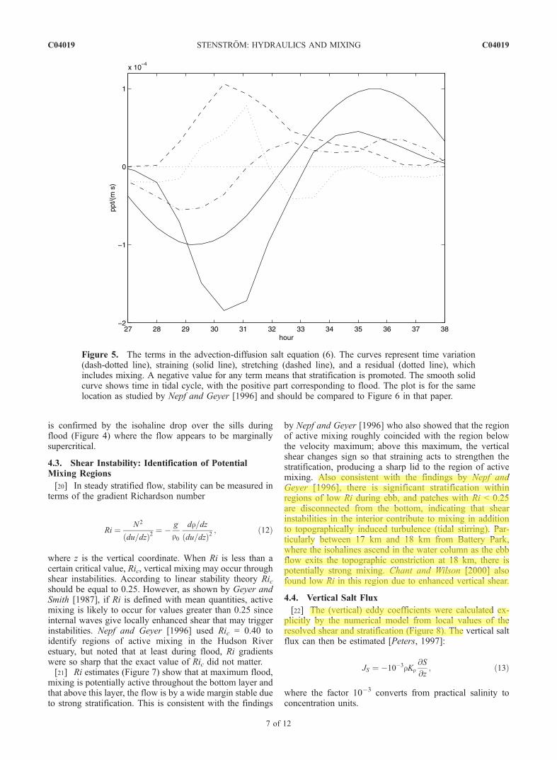
On the right-hand side, the first term represents straining,the second stretching, and the third diffusion of the salinityfield. Cross-channel terms are neglected and the along-channel salinity gradient and velocity are considereduniform. To facilitate comparison to Nepf and Geyer[1996], we focus on the near-bed region, defined as thebottom 40% of the local depth. Vertical derivatives weresimply estimated as the difference between the top andbottom of this region and the horizontal derivative as thecentral difference over 60 grid points (2250 m). The termsof equation (6) are plotted in Figure 5. Consistent with Nepfand Geyer [1996], the temporal variation is dominated bytidal straining. Straining promotes stratification during ebband diminishes stratification during flood. There is anasymmetry so that the tidally averaged straining is negative,representing the straining induced by the mean estuarinecirculation. The stretching term, which represents thevertical stretching of the salinity field due to differentialvertical advection, counteracts straining during ebb anddiminishes stratification. The magnitudes of these termsvery closely resemble those calculated from data by Nepfand Geyer [1996].

4.2. Two-Layer Model: Analysis of Halocline Behavior

[17] To analyze the hydraulics of the flow we shall followChant and Wilson [2000] and derive an expression for the

along-channel slope of the interface in an inviscid two-layerflow (noting that an inviscid, energy-conserving descriptionwill only capture some aspects of a continuously stratified,viscous flow, and that any quantitative statements areuncertain). Starting from the Bernoulli equations for aninviscid two-layer flow in a channel,

u212g

þ H þ h1 þ h2 ¼ C1 ð7aÞ

u222g

þ H þ h2 þr1r2h1 ¼ C2; ð7bÞ

where Ci are constants, H is the bottom elevation abovesome datum, and ri, hi, and ui are the density, thickness, andvelocity of layer i, respectively, subtracting equation (7b)from equation (7a) and using the continuity equation, qi =uiBhi, to replace the layer velocities with layer discharges,we get

1

2g

q21B2h21

� q22B2h22

� �þ r2 � r1

r2h1 ¼ C; ð8Þ

where B is the (vertically uniform) channel width.Differentiating with respect to the along-channel direction,

Figure 3. Comparison between measured and modeled profiles at (top) maximum ebb and (bottom)maximum flood for CTD stations (left) 1, (middle) 7, and (right) 10. Solid lines show streamwisevelocity, and dashed lines show salinity. Thin lines show measured profiles, and bold lines show modeledprofiles. Positive velocities are up-estuary.

C04019 STENSTROM: HYDRAULICS AND MIXING

5 of 12

C04019

x (positive up-estuary), and again using the continuityequation to make the layer velocities explicit variables,gives

� u21h1g

@h1@x

� u21Bg

@B

@xþ u22h2g

@h2@x

þ u22Bg

@B

@xþ r2 � r1

r2

@h1@x

¼ 0:

ð9Þ

Substituting the layer Froude number Fi2 = ui

2/(g0hi) andmultiplying by g/g0, equation (9) can be written as

�F21

@h1@x

þ F22

@h2@x

þ 1

Bg0@B

@xu22 � u21

þ @h1@x

¼ 0: ð10Þ

Substituting @h2/@x = �(@H/@x + @h1/@x), we get anexpression for the along-channel rate of change of upperlayer thickness (indirectly slope of the interface):

@h1@x

¼F22

@H

@xþ 1

Bg0@B

@xu21 � u22

1� G2ð Þ : ð11Þ

[18] The subdivision of the simulated (continuous) flowinto two discrete layers for estimation of layer velocitiesand Froude numbers can be made in several ways. First,isotachs and isohalines do not coincide when mixing isactive, and therefore a choice has to be made whether tobase the subdivision on the velocity field or the salinity

field. Second, the halocline is not sharp over the entiretidal cycle; rather, the stratification is almost linear duringebb. It was chosen here to use the 9 ppt isohaline toapproximate the interface. This is a somewhat arbitrarychoice, but the estimation of Froude numbers was foundnot to be very sensitive to the choice of subdivision. Thereduced gravity, g0, was calculated at every point along thechannel from the difference between the average densitiesof the layers at that point. The Froude numbers are plottedin Figure 6.[19] The isohalines make large vertical excursions pri-

marily at maximum ebb and maximum flood (compareFigure 4). At maximum ebb, the isohalines drop sharplyas the flow enters the lateral contractions just downstream ofthe two sills (compare Figure 2). Returning to equation (11)and Figure 2, we note that @H/@x and @B/@x tend to havethe same sign. Therefore when the surface layer velocitiesexceed the bottom layer velocities, as is the case during ebb,the two terms are of the same sign. If the flow is supercrit-ical (G2 > 1), then when the channel deepens (@H/@x < 0)and contracts (@B/@x < 0), the two terms will both act toincrease the thickness of the surface layer. Conversely,when the channel shoals and expands, the two terms willact to decrease the thickness of the surface layer. Duringflood, bottom layer velocities exceed or equal surface layervelocities and the two terms will be of opposite signs andthus act in conflict on the surface layer. However, thesecond term will in general be small since the differencebetween surface and bottom layer velocities is small duringflood, and the first term is thus expected to dominate. This

Figure 4. Modeled salinity contours.

C04019 STENSTROM: HYDRAULICS AND MIXING

6 of 12

C04019

is confirmed by the isohaline drop over the sills duringflood (Figure 4) where the flow appears to be marginallysupercritical.

4.3. Shear Instability: Identification of PotentialMixing Regions

[20] In steady stratified flow, stability can be measured interms of the gradient Richardson number

Ri ¼ N2

du=dzð Þ2¼ � g

r0

dr=dz

du=dzð Þ2; ð12Þ

where z is the vertical coordinate. When Ri is less than acertain critical value, Ric, vertical mixing may occur throughshear instabilities. According to linear stability theory Ricshould be equal to 0.25. However, as shown by Geyer andSmith [1987], if Ri is defined with mean quantities, activemixing is likely to occur for values greater than 0.25 sinceinternal waves give locally enhanced shear that may triggerinstabilities. Nepf and Geyer [1996] used Ric = 0.40 toidentify regions of active mixing in the Hudson Riverestuary, but noted that at least during flood, Ri gradientswere so sharp that the exact value of Ric did not matter.[21] Ri estimates (Figure 7) show that at maximum flood,

mixing is potentially active throughout the bottom layer andthat above this layer, the flow is by a wide margin stable dueto strong stratification. This is consistent with the findings

by Nepf and Geyer [1996] who also showed that the regionof active mixing roughly coincided with the region belowthe velocity maximum; above this maximum, the verticalshear changes sign so that straining acts to strengthen thestratification, producing a sharp lid to the region of activemixing. Also consistent with the findings by Nepf andGeyer [1996], there is significant stratification withinregions of low Ri during ebb, and patches with Ri < 0.25are disconnected from the bottom, indicating that shearinstabilities in the interior contribute to mixing in additionto topographically induced turbulence (tidal stirring). Par-ticularly between 17 km and 18 km from Battery Park,where the isohalines ascend in the water column as the ebbflow exits the topographic constriction at 18 km, there ispotentially strong mixing. Chant and Wilson [2000] alsofound low Ri in this region due to enhanced vertical shear.

4.4. Vertical Salt Flux

[22] The (vertical) eddy coefficients were calculated ex-plicitly by the numerical model from local values of theresolved shear and stratification (Figure 8). The vertical saltflux can then be estimated [Peters, 1997]:

JS ¼ �10�3rKr@S

@z; ð13Þ

where the factor 10�3 converts from practical salinity toconcentration units.

Figure 5. The terms in the advection-diffusion salt equation (6). The curves represent time variation(dash-dotted line), straining (solid line), stretching (dashed line), and a residual (dotted line), whichincludes mixing. A negative value for any term means that stratification is promoted. The smooth solidcurve shows time in tidal cycle, with the positive part corresponding to flood. The plot is for the samelocation as studied by Nepf and Geyer [1996] and should be compared to Figure 6 in that paper.

C04019 STENSTROM: HYDRAULICS AND MIXING

7 of 12

C04019

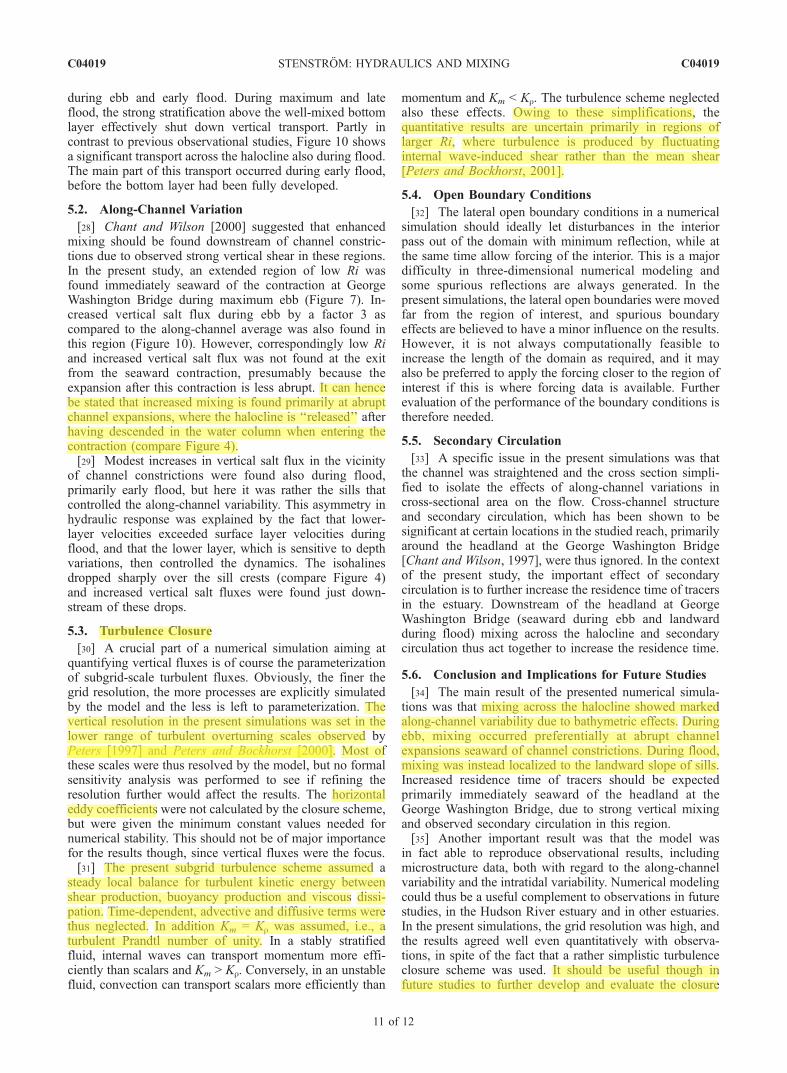
[23] Figure 9 shows modeled profiles of vertical salt flux,averaged over flood and ebb respectively, for the samelocation in the vicinity of station 1 (compare Figure 1)where Peters and Bockhorst [2001] estimated salt flux frommicrostructure data (compare Figure 7a in their paper)and where Nepf and Geyer [1996] estimated salt flux based

on a Munk-Anderson parameterization of Kr and observedsalinity gradients (compare Figure 10 in their paper).Consistent with their estimates, the maximum values arefound close to the bottom where vertical shear is strong. Themaximum modeled values are in the same order of magni-tude as the estimates of Peters and Bockhorst [2001], but

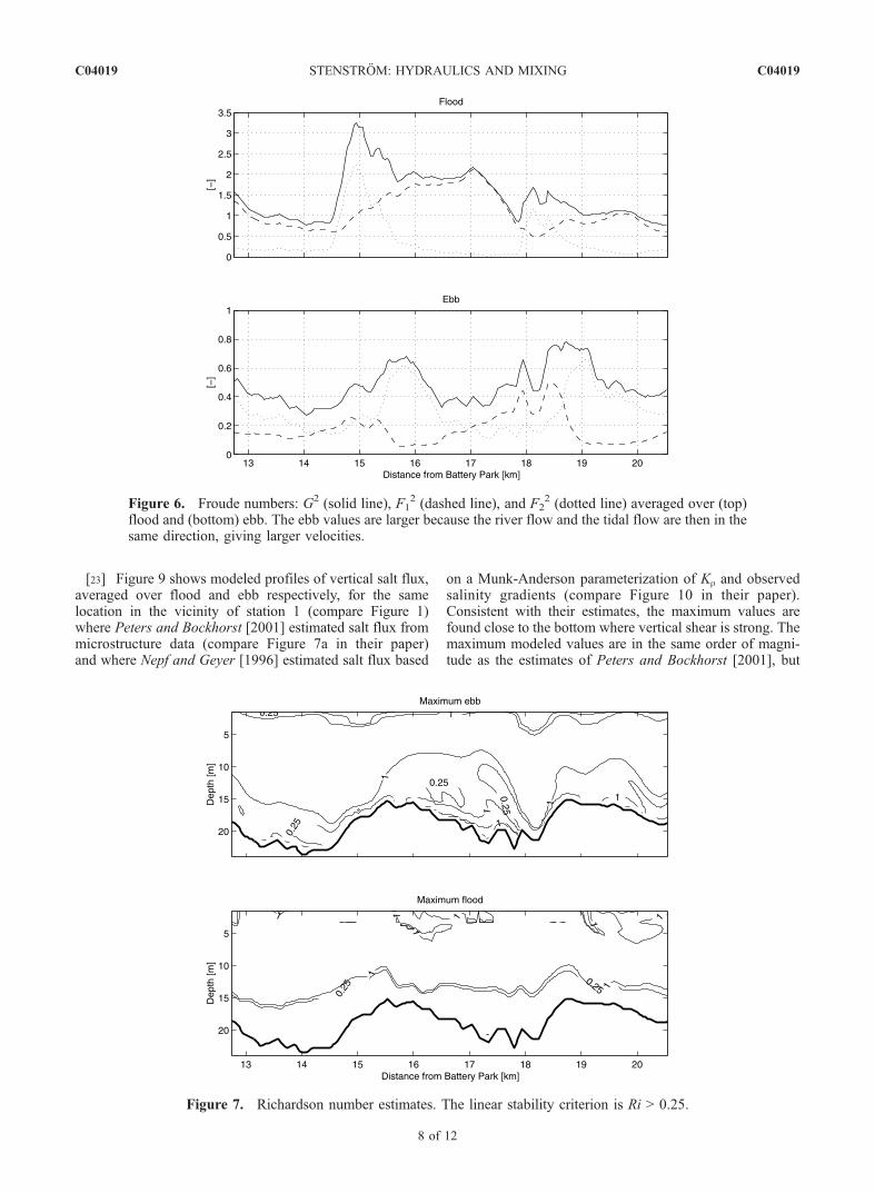
Figure 7. Richardson number estimates. The linear stability criterion is Ri > 0.25.

Figure 6. Froude numbers: G2 (solid line), F12 (dashed line), and F2

2 (dotted line) averaged over (top)flood and (bottom) ebb. The ebb values are larger because the river flow and the tidal flow are then in thesame direction, giving larger velocities.

C04019 STENSTROM: HYDRAULICS AND MIXING

8 of 12

C04019

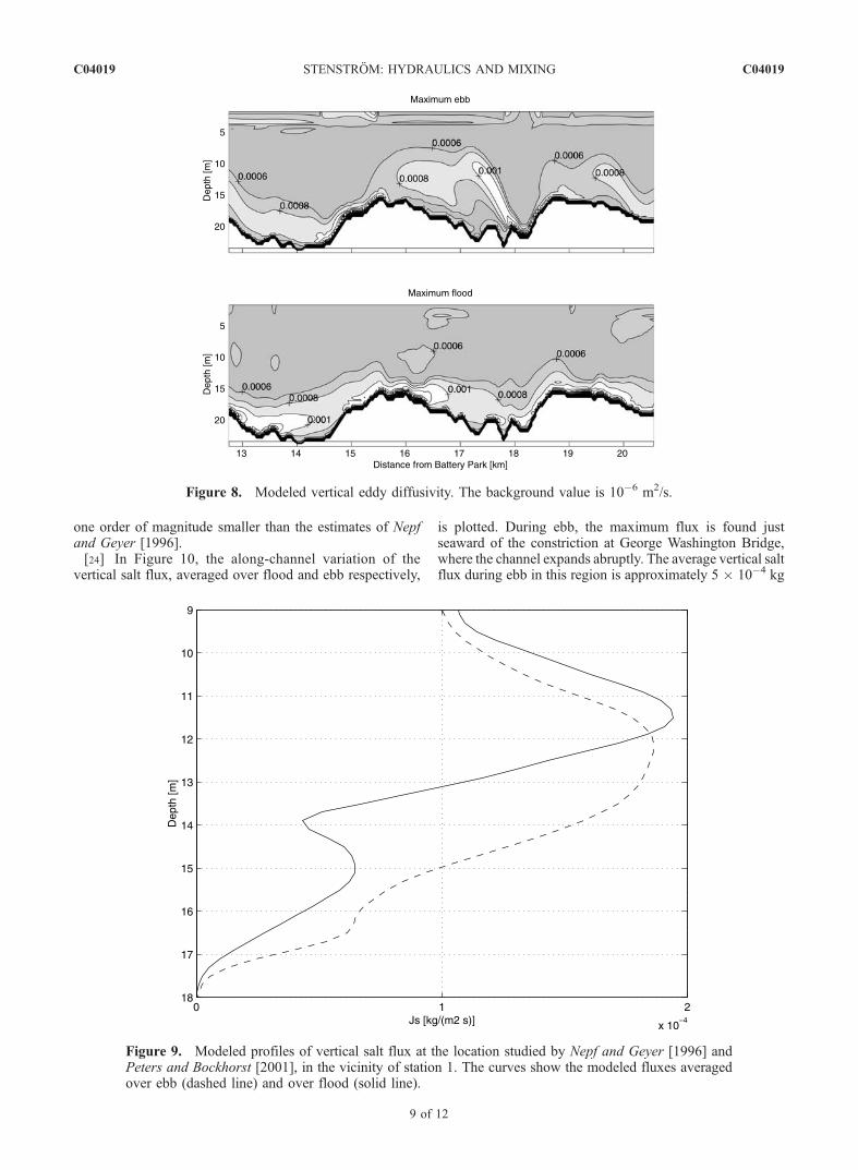
one order of magnitude smaller than the estimates of Nepfand Geyer [1996].[24] In Figure 10, the along-channel variation of the

vertical salt flux, averaged over flood and ebb respectively,

is plotted. During ebb, the maximum flux is found justseaward of the constriction at George Washington Bridge,where the channel expands abruptly. The average vertical saltflux during ebb in this region is approximately 5 � 10�4 kg

Figure 9. Modeled profiles of vertical salt flux at the location studied by Nepf and Geyer [1996] andPeters and Bockhorst [2001], in the vicinity of station 1. The curves show the modeled fluxes averagedover ebb (dashed line) and over flood (solid line).

Figure 8. Modeled vertical eddy diffusivity. The background value is 10�6 m2/s.

C04019 STENSTROM: HYDRAULICS AND MIXING

9 of 12

C04019

m�2 s�1, corresponding to an increase by a factor 3 ascompared to the along-channel average. No increase in saltflux is seen downstream of the seaward constriction, pre-sumably because the expansion after this constriction is lessabrupt. During flood, regions with moderately enhancedvertical fluxes are found on the landward side of the twosills. The sills are more important during flood since lowerlayer velocities then exceed surface layer velocities. Thelower layer, which is sensitive to depth variations, thencontrols the dynamics. Conversely, during ebb, surface layervelocities are greater and the dynamics are controlled by thesurface layer, which feels only width variations.

5. Discussion

[25] A nonhydrostatic three-dimensional numerical modelwas set up to study intratidal and along-channel variabilityin stratification and mixing during neap tide conditions inthe Hudson River estuary. Three-dimensional modeling of afull tidal cycle has to the author’s knowledge not been triedbefore for this estuary. The modeled fields showed goodagreement with data, although the fit could most likely beimproved by more systematic data assimilation and withbetter information about velocity and salinity distribution atthe upstream and downstream boundaries. The simulationsconfirmed many of the results from earlier, purely observa-tional studies in the Hudson River estuary and in additionallowed the along-channel variation in vertical salt flux tobe explored over the tidal cycle. Numerical modeling hasthe advantage that the results cover the dynamics withoutbias to particular sampling times in the tidal cycle. Numer-ical modeling also allows the relative magnitude of differentforcing components to be systematically varied and theestuary response to be studied. The latter was however

beyond the scope of the present paper. The results arediscussed below, followed by a discussion of a few impor-tant issues that need to be further explored in order toincrease the quantitative confidence in numerical results.

5.1. Intratidal Variation

[26] The simulated fields were found to be clearly domi-nated by estuarine circulation, with maintained stratificationover the entire tidal cycle. Tidal straining was found todominate the intratidal variability in that maximum andminimum near-bed stratification occurred during late ebband late flood respectively. Regions with potentially activemixing, identified by lowRi, were confined to the well-mixedbottom layer during maximum and late flood, whereas duringebb and early flood, patches of low Ri and potentially activemixing were found also in the stratified interior of the fluid.These patches indicate that shear instabilities in the interiorcontributed to mixing in addition to topography-inducedturbulence.[27] The expression for the vertical eddy coefficients,

equation (3), can be rewritten in terms of Ri:

Km;r ¼ CSDð Þ2Tffiffiffiffiffiffiffiffiffiffiffiffiffi1� Ri

p; T ¼

ffiffiffiffiffiffiffiffiffiffiffiffiffiffiffiffiffiffiffiffiffiffiffiffiffiffiffiffiffiffiffiffiffiffiffiffiffiffiffi@v=@zð Þ2þ @v=@zð Þ2

q: ð14Þ

When Ri > 1, the square root argument is negative and theviscosity is set to the background viscosity. It is clear fromequation (14) and from Figures 7 and 8 that Ri and Km,rfollow each other closely; low Ri corresponds to high Km,rand vice versa. The expression for the vertical salt flux, JS,contains the product of Kr and the salinity gradient, but thevariability of Kr was much larger, so increased vertical saltflux was found only in areas of high Kr and low Ri. Verticalsalt flux above the bottom layer was hence significant only

Figure 10. Along-channel variation in vertical salt flux equation (13), averaged over (top) ebb and(bottom) flood and for the 8 and 10 ppt isohalines. The dashed lines show the along-channel averages.

C04019 STENSTROM: HYDRAULICS AND MIXING

10 of 12

C04019

during ebb and early flood. During maximum and lateflood, the strong stratification above the well-mixed bottomlayer effectively shut down vertical transport. Partly incontrast to previous observational studies, Figure 10 showsa significant transport across the halocline also during flood.The main part of this transport occurred during early flood,before the bottom layer had been fully developed.

5.2. Along-Channel Variation

[28] Chant and Wilson [2000] suggested that enhancedmixing should be found downstream of channel constric-tions due to observed strong vertical shear in these regions.In the present study, an extended region of low Ri wasfound immediately seaward of the contraction at GeorgeWashington Bridge during maximum ebb (Figure 7). In-creased vertical salt flux during ebb by a factor 3 ascompared to the along-channel average was also found inthis region (Figure 10). However, correspondingly low Riand increased vertical salt flux was not found at the exitfrom the seaward contraction, presumably because theexpansion after this contraction is less abrupt. It can hencebe stated that increased mixing is found primarily at abruptchannel expansions, where the halocline is ‘‘released’’ afterhaving descended in the water column when entering thecontraction (compare Figure 4).[29] Modest increases in vertical salt flux in the vicinity

of channel constrictions were found also during flood,primarily early flood, but here it was rather the sills thatcontrolled the along-channel variability. This asymmetry inhydraulic response was explained by the fact that lower-layer velocities exceeded surface layer velocities duringflood, and that the lower layer, which is sensitive to depthvariations, then controlled the dynamics. The isohalinesdropped sharply over the sill crests (compare Figure 4)and increased vertical salt fluxes were found just down-stream of these drops.

5.3. Turbulence Closure

[30] A crucial part of a numerical simulation aiming atquantifying vertical fluxes is of course the parameterizationof subgrid-scale turbulent fluxes. Obviously, the finer thegrid resolution, the more processes are explicitly simulatedby the model and the less is left to parameterization. Thevertical resolution in the present simulations was set in thelower range of turbulent overturning scales observed byPeters [1997] and Peters and Bockhorst [2000]. Most ofthese scales were thus resolved by the model, but no formalsensitivity analysis was performed to see if refining theresolution further would affect the results. The horizontaleddy coefficients were not calculated by the closure scheme,but were given the minimum constant values needed fornumerical stability. This should not be of major importancefor the results though, since vertical fluxes were the focus.[31] The present subgrid turbulence scheme assumed a

steady local balance for turbulent kinetic energy betweenshear production, buoyancy production and viscous dissi-pation. Time-dependent, advective and diffusive terms werethus neglected. In addition Km = Kr was assumed, i.e., aturbulent Prandtl number of unity. In a stably stratifiedfluid, internal waves can transport momentum more effi-ciently than scalars and Km > Kr. Conversely, in an unstablefluid, convection can transport scalars more efficiently than

momentum and Km < Kr. The turbulence scheme neglectedalso these effects. Owing to these simplifications, thequantitative results are uncertain primarily in regions oflarger Ri, where turbulence is produced by fluctuatinginternal wave-induced shear rather than the mean shear[Peters and Bockhorst, 2001].

5.4. Open Boundary Conditions

[32] The lateral open boundary conditions in a numericalsimulation should ideally let disturbances in the interiorpass out of the domain with minimum reflection, while atthe same time allow forcing of the interior. This is a majordifficulty in three-dimensional numerical modeling andsome spurious reflections are always generated. In thepresent simulations, the lateral open boundaries were movedfar from the region of interest, and spurious boundaryeffects are believed to have a minor influence on the results.However, it is not always computationally feasible toincrease the length of the domain as required, and it mayalso be preferred to apply the forcing closer to the region ofinterest if this is where forcing data is available. Furtherevaluation of the performance of the boundary conditions istherefore needed.

5.5. Secondary Circulation

[33] A specific issue in the present simulations was thatthe channel was straightened and the cross section simpli-fied to isolate the effects of along-channel variations incross-sectional area on the flow. Cross-channel structureand secondary circulation, which has been shown to besignificant at certain locations in the studied reach, primarilyaround the headland at the George Washington Bridge[Chant and Wilson, 1997], were thus ignored. In the contextof the present study, the important effect of secondarycirculation is to further increase the residence time of tracersin the estuary. Downstream of the headland at GeorgeWashington Bridge (seaward during ebb and landwardduring flood) mixing across the halocline and secondarycirculation thus act together to increase the residence time.

5.6. Conclusion and Implications for Future Studies

[34] The main result of the presented numerical simula-tions was that mixing across the halocline showed markedalong-channel variability due to bathymetric effects. Duringebb, mixing occurred preferentially at abrupt channelexpansions seaward of channel constrictions. During flood,mixing was instead localized to the landward slope of sills.Increased residence time of tracers should be expectedprimarily immediately seaward of the headland at theGeorge Washington Bridge, due to strong vertical mixingand observed secondary circulation in this region.[35] Another important result was that the model was

in fact able to reproduce observational results, includingmicrostructure data, both with regard to the along-channelvariability and the intratidal variability. Numerical modelingcould thus be a useful complement to observations in futurestudies, in the Hudson River estuary and in other estuaries.In the present simulations, the grid resolution was high, andthe results agreed well even quantitatively with observa-tions, in spite of the fact that a rather simplistic turbulenceclosure scheme was used. It should be useful though infuture studies to further develop and evaluate the closure

C04019 STENSTROM: HYDRAULICS AND MIXING

11 of 12

C04019

scheme [e.g., Nunes Vaz and Simpson, 1994], particularlyfor studies where a coarser grid resolution has to be used forcomputational feasibility. The extensive data sets from theHudson River estuary, covering along-channel variability aswell as intratidal and neap to spring variability, provide agood basis for such an evaluation.

[36] Acknowledgments. These studies were started when I was on a3 month visit at the Marine Sciences Research Center, State University ofNew York at Stony Brook, October–December 2000. I would like to thankRobert E. Wilson for introducing me to this subject and for giving meaccess to data from the field measurements. I would also like to thankAnders Engqvist for helpful comments on the manuscript and GoranBrostrom for assistance when setting up the numerical experiment on the48-processor Linux cluster that he built. Thanks also to two anonymousreviewers, who contributed to major improvements of the manuscript.

ReferencesAdcroft, A. (1997), Representation of topography by shaved cells in aheight coordinate ocean model, Mon. Weather Rev., 125, 2293–2315.

Chant, R. J., and R. E. Wilson (1997), Secondary circulation in a highlystratified estuary, J. Geophys. Res., 102, 23,207–23,215.

Chant, R. J., and R. E. Wilson (2000), Internal hydraulics and mixing in ahighly stratified estuary, J. Geophys. Res., 105, 14,215–14,222.

Geyer, W. R., and J. D. Smith (1987), Shear instability in a highly stratifiedestuary, J. Phys. Oceanogr., 17, 1668–1679.

Jay, D. A., and J. D. Smith (1990), Residual circulation in shallow estuaries:1. Highly stratified, narrow estuaries, J. Geophys. Res., 95, 711–731.

Khatiwala, S. (2003), Generation of internal tides in an ocean of finitedepth: Analytical and numerical calculations, Deep Sea Res., Part I,50, 3–21.

Marshall, J., A. Adcroft, C. Hill, L. Perelman, and C. Heisey (1997), Afinite-volume, incompressible Navier Stokes model for studies of theocean on parallel computers, J. Geophys. Res., 102, 5753–5766.

Nepf, H. M., and W. R. Geyer (1996), Intratidal variations in stratificationand mixing in the Hudson estuary, J. Geophys. Res., 101, 12,079–12,086.

Nunes Vaz, R. A., and J. H. Simpson (1994), Turbulence closure modelingof estuarine stratification, J. Geophys. Res., 99, 16,143–16,160.

Nunes Vaz, R. A., G. W. Lennon, and J. R. de Silva Samarasinghe (1989),The negative role of turbulence in estuarine mass transport, EstuarineCoastal Shelf Sci., 28, 361–377.

Nycander, J., and K. Doos (2003), Open boundary conditions for barotropicwaves, J. Geophys. Res., 108(C5), 3168, doi:10.1029/2002JC001529.

Orlanski, I. (1976), A simple boundary condition for unbounded hyperbolicflows, J. Comput. Phys., 21, 251–269.

Peters, H. (1997), Observations of stratified turbulent mixing in an estuary:Neap-to-spring variations during high river flow, Estuarine Coastal ShelfSci., 45, 69–88.

Peters, H. (2003), Broadly distributed and locally enhanced turbulentmixing in a tidal estuary, J. Phys. Oceanogr., 33, 1967–1977.

Peters, H., and R. Bockhorst (2000), Microstructure observations of turbu-lent mixing in a partially mixed estuary: 1. Dissipation rate, J. Phys.Oceanogr., 30, 1232–1244.

Peters, H., and R. Bockhorst (2001), Microstructure observations of turbu-lent mixing in a partially mixed estuary: 2. Salt flux and stress, J. Phys.Oceanogr., 31, 1105–1119.

Rodi, W. (1987), Examples of calculation methods for flow and mixing instratified fluids, J. Geophys. Res., 92, 5305–5328.

Simpson, J. H., J. Brown, J. P. Matthews, and G. Allen (1990), Tidalstraining, density currents and stirring in the control of estuarine stratifi-cation, Estuaries, 13, 125–132.

Smagorinsky, J. (1963), General circulation experiments with the primitiveequations, Mon. Weather Rev., 91, 99–164.

Stenstrom, P. (2003), Mixing and recirculation in two-layer exchange flows,J. Geophys. Res., 108(C8), 3256, doi:10.1029/2002JC001696.

Ullman, D. S., and R. E. Wilson (1998), Model parameter estimation fromdata assimilation modeling: Temporal and spatial variability of thebottom drag coefficient, J. Geophys. Res., 103, 5531–5549.

Winters, K. B., and H. E. Seim (2000), The role of dissipation and mixingin exchange flow through a contracting channel, J. Fluid Mech., 407,265–290.

�����������������������P. Stenstrom, Department of Land and Water Resources Engineering,

Royal Institute of Technology, SE-10044 Stockholm, Sweden. (petters@kth.se)

C04019 STENSTROM: HYDRAULICS AND MIXING

12 of 12

C04019