Hybrid Tracking using Dempster-Shafer Data Fusion in Real-Time Augmented Reality Applications

for Man-Made Environments

Betül AYDIN

Advisor: Prof. Bruno TELLEZ

LIRIS (Laboratoire d‟InfoRmatique en Image et Systèmes d‟information)

UMR 5205 CNRS/Université Claude Bernard Lyon 1

43, Boulevard du 11 novembre 1918, 69622 Villeurbanne Cedex - France

betul.aydin@insa-lyon.fr, bruno.tellez@liris.cnrs.fr

Abstract. In this report, we present a real-time hybrid tracking system for

augmented reality applications in urban environments. In our framework, the

augmented model aligns itself on the building planar surfaces by using several

vision based tracking information, such as corner points, vanishing points and

homography between images. In addition to the vision based alignment, the

method uses the inner sensor data of the mobile phone as a feedback. We

estimate the search space of the feature locations for the next frames using the

history of previous states with the help of gyroscope and accelerometer data and

as well as the vision tracking information. We combine these data by using a

probabilistic approach defined by Dempster-Shafer. The different stages of the

approach are demonstrated on various examples of building images.

Keywords: augmented reality, architectural environment, man-made structures,

vanishing point detection, homography between images, dempster-shafer data

fusion

Résumé. Dans ce rapport, nous proposons un système de suivi hybride en

temps réel pour des applications de réalité augmentée dans les environnements

urbains. Dans ce cadre, le modèle de réalité augmenté s'aligne sur les surfaces

planaires de bâtiment en s‟appuyant sur le suivi d‟information basées sur la

vision, telles que les coins d‟angle, les points de fuite et l‟homographie entre les

images. En plus de l'alignement basé sur la vision, la méthode utilise les

données des capteurs internes du téléphone mobile pour améliorer la qualité de

l‟alignement. Nous estimons l'espace de point d‟intérêts dans les images

suivantes en établissant l‟historique des états précédents grâce aux données du

gyroscope et de l‟accéléromètre ainsi que les informations issu du suivi visuel

de ce point dans la théorie de Dempster-Shafer. Les différentes étapes de notre

approche seront détaillées sur divers exemples d‟images urbains.

Mots clé: réalité augmentée, l'environnement architectural, structures

artificielles les points de fuite, homographie entre les images, Dempster-Shafer

fusion de données

2

1 Introduction ................................................................................................. 2

2 State of Art .................................................................................................. 3

2.1 Knowledge of position and orientation of the camera ........................... 3

2.2 Tracking features/objects/surfaces in the image .................................... 5

2.3 Defining 3D camera motion based on the tracked features .................... 7

2.4 Vanishing Point Detection ................................................................... 9

2.5 Data Fusion by Using Dempster-Shafer Theory .................................. 10

3 Description of the work .............................................................................. 12

3.1 Vanishing Point Detection ................................................................. 13

3.2 Corner Detection and Tracking .......................................................... 20

3.3 Homography between images ............................................................ 21

3.3.1 Computation of ..................................................................... 23

3.4 Inner sensors contribution .................................................................. 24

3.5 Overall Scenario ................................................................................ 26

3.5.1 Algorithm Summary ...................................................................... 26

3.5.2 Contributions to the scenario: ........................................................ 27

3.6 Data fusion with Dempster-Shafer Theory.......................................... 27

4 Conclusion ................................................................................................ 29

References ......................................................................................................... 30

1 Introduction

The aim of this report is to review the state of art of the augmented reality

applications related with images/videos taken by mobile phones in urban areas by

referring to their current capabilities and limitations. The report is based on review of

the current literature, the description of the project that built on this review and the

detailed explanation of the proposed solution. The project itself consists of the

contributions of different methods frequently used in augmented reality applications

such as finding homographies between images or tracking feature points in videos.

With the increasing demand and supply of mobile phones, several mobile

application scenarios have arisen. Today, high resolution built-in cameras, inner

sensors and Global Positioning System (GPS) are indispensible within mobile phones.

3

Our work focuses on the real-time analysis of architectural environments in mobile

applications. Urban areas can be characterized by many parallel lines and orthogonal

edges. For building recognition and detection, this information has been the key-point

for researchers while they were treating urban data.

2 State of Art

The advances in computer vision and mobile computing have let the augmented

reality systems to emerge from indoor applications to outdoor applications [1]. The

purpose of an outdoor augmented reality application is to allow the user to freely

interact with the surrounding environment in real-time with digital cameras or mobile

phones which could possibly have accelerometers, GPS, gyroscopes or wireless

sensors. The application areas of augmented reality may vary from tourism,

entertainment, leisure, architecture, construction industry, navigation, education etc…

However, the position and orientation of the camera are challenging and essential

information to gather for the augmented reality applications. As well as being not so

accurate, current GPS technology is the prior knowledge to estimate the position of

the user. The second challenge is to track the camera position with the help of the

reference points from the scene (vision-based tracking), as well as maybe with the

help of GPS, digital compass and accelerometers. There are many geometric

approaches to define 3D camera motion based on mathematical constraints, which

calculate the fundamental matrix by using multiple images, in order to define the

motion between two frames of the same static scene [2]. There are also several ways

to define the reference points in the scene. Here, we will go over those aspects and

explain why every approach cannot be suitable for real-time mobile applications.

Tracking methods have broad application areas and it is one of the prior knowledge

in augmented reality to be able to locate the models in the images or videos. We will

examine the current state of art in five titles. First, we will explain how the camera

location and orientation can be estimated without using the vision-based data.

Secondly, we will give some examples to object tracking algorithms that are broadly

used for the alignment of the virtual model into the scene. Next, we will look at the

vision-based tracking methods that are used to model the camera motion in the scene,

as well as the methods that integrate the sensor data with the vision-based tracking.

Then, we will introduce a characteristic of urban environments that helps to

understand the geometry of the scene. Finally, we will explain a probabilistic method

to sum up those approaches in a way that the method will employ the most trustable

data (vision-based or sensor-based) according to the current state of the application.

2.1 Knowledge of position and orientation of the camera

Visualizing virtual models in real world locations in real-time has enabled mobile

augmented reality applications to broaden and become a promising area for research.

By using user‟s viewpoint, the virtual 3D objects (text, models, or images) appear as

if they are in the real environment and take place at the intended world positions [4],

4

[5]. Defining exact viewpoint position and orientation cannot be thought separately

from tracking technologies, since it highly depends on the qualities of the mobile

device (GPS, different sensors, wireless infrastructure) [4]. With the user‟s position

and orientation in space-time, it is possible to place the models in geo coordinates. At

this point, tracking feature points in the images have let more interaction with the

physical environment, such as locating the model on the correct geo coordinates as

well as with the correct altitude and orientation; we will return to these points later.

Visual tracking by sensors like gyroscopes, accelerometers and GPS modules is not

very accurate. However they have been used widely for first estimation of the camera

pose. B. Reitinger et al. propose combination of sensors for modeling urban sites [6].

They use on-line generation of 3D models with handheld ultra-mobile PCs. With GPS

information, the resulting models can be available in geographic coordinate systems.

The user then takes pictures of the buildings while exploring the environment and

those images are enriched by current positioning data (taken from a GPS receiver) and

then sent to the database for further processing. However, it is known that current

GPS information has a precision of up to 20-50 meters depending on the area and

weather conditions.

Another application, photo explorer, allows virtual tourism of the world‟s

interesting and important sites [7]. By using geo-location information, the photos can

be registered on the map correctly. Unordered set of photos are registered by the user

and the application is presented in an interactive 3D browser. This kind of photo

tourism applications are in demand and it enables users to make tours in scenic or

historic locations by viewing their locations on the map. In these kinds of

applications, the location of the camera is generally obtained from GPS or manually

specified by the user. Also, in some cases, like in their application there is no request

for the GPS since after the user uploads the photo to the server, the photo is compared

to an image database and location information is received from database. These kinds

of applications are mainly available for the touristic, well-known sites which photos

already exist in the database with the navigation information; so that newly taken

photos can be compared and located on the map. However, if it is not applicable for

the unknown scenes where GPS information is needed to locate the user, these

estimated camera locations are related to the absolute locations through a global

translation, rotation and uniform scale. To determine the correct transformation, the

user asked to rotate, translate and scale the image until it is aligned. This kind of

interaction is not applicable for the real-time video augmented reality applications.

Also, another disadvantage is that, if there is a need of tracking in the video, the

matching algorithms may slow down the application.

In a recent work [8], a multi-sensor fusion is proposed for the user‟s 3D position

estimation. As it is highlighted in the article, the precision and update rate of the

current GPS technologies are not sufficient for high quality of tracking. Therefore,

they develop a multi-sensor fusion to track the user‟s position in outdoor

environments. They employ Kalman filtering for fusion of Differential GPS and

inertial measurement units with gyroscopes, magnetometers and accelerometers for

improvements. In order to avoid distortion, they apply a visual orientation tracker

which increases the robustness and accuracy of the pose estimates. Dense building

5

blocks in urban environments degrade GPS accuracy and the roof structures may lead

to drop outs in position updates from GPS. In their work, they build a handheld

outdoor AR platform and include a magnetic compass which provides a convenient

absolute orientation with respect to earth‟s magnetic field. Also, they employ

gyroscopes to estimate the rotational velocity and linear accelerometers for the

estimation of gravity or vision-based tracking. However, for mobile applications,

since already implemented sensors are used, the applicability of the proposed methods

is limited and depends on the features of the sensors of the mobile. Smartphones are

rather delicate, miniature computers that have diverse functionalities; however they

cannot be as efficient and fast as handheld outdoor AR platforms that are made up of

the combinations of highly accurate sensors. Also, the visual tracking methods may

greatly influence the performance of the application which is not explained in detail

even if it is one of the methods used in their application.

As a mini-PC equipment implementation, [9] user puts an virtual 3D model in

video of a scene. They use Google Earth KML files as well as GPS. Keyhole Markup

Language (KML) is a file format to display geographic data in 2D maps or 3D Earth

browsers. According to that, while the person uses the camera, the position of the user

is detected by using GPS and then the object (ex: a 3D building) is located with a

knowledge of its global position on the map. The building, since its 3D position is

determined by the user before, stays on its position and while the user changes its

position, the distance and the compass direction are calculated. The direction of the

building is known since it is placed on the 3D global map. Then the relative position

of the building to the user is calculated, and the virtual building is placed on the right

distance and orientation. As it is pointed in this work, in video-based augmented

reality applications, the alignment of 3D (or 2D) model with the video of the real

scene is challenging. We have to know the camera position and orientation relative to

the scene. In their proposition, the user places the 3D model to the scene and it is

assumed that the user does not change his viewing location but just turns the camera.

So that, the tracking is simplified and they analyze the horizontal and vertical pixel

movements caused by the rotation of the camera. In this project, since they are

placing huge objects to the far points in the scene, the accuracy of the altitude of the

camera is not so important (they use 1.7m as default). However, in applications,

where small models are placed into the scene, (a sticker on a building) the precise

altitude information is important. Therefore, this method is not applicable for our

project, since accuracy has priority. The key requirement for our project is a tracking

system where the position and orientation are calculated in a way that it is enough to

make the illusion for the placement of the virtual model in the scene. Also, for the

purpose of our object, we are interested in making this illusion of locating the camera

viewpoint in architectural environments.

2.2 Tracking features/objects/surfaces in the image

In augmented reality applications, the tracking of interested regions is the

fundamental information to place the virtual model in the scene correctly since the

region imposes a reference for the placement and the alignment of the virtual object.

6

Also, tracking might be useful in some applications to detect the camera position,

orientation and motion that we will mention in the next section.

There are various augmented reality scenarios in which the camera is static and the

tracked object/region is moving in the scene; or the scene is static and the observer is

moving; or both are moving. Tracking feature points enables to estimate the pose of

the scene so that the model will be integrated correctly into the scene. In some

applications [10], [11], [12], where the scene is static and the camera is moving, they

place the model by tracking the fiducials (artificial markers) in the scene, also they

benefit from these features to estimate the camera motion in the scene. With the fact

that placing artificial markers is not available in unprepared outdoor environments, it

is still possible to extract the camera motion from feature-based (markerless) tracking

that we will mention in the following sections.

In object tracking, an object can be defined as anything that is of interest for further

analysis; such as points, primitive geometric shapes, object silhouettes and contours

[22]. The choice of object representation depends on the application domain. In our

project, we are working in outdoor environments where mostly geometric shapes

(buildings) take place in the images. Therefore, the motion will be in the form of

translation, rotation, affine or projective (homography) transformation.

One of the earliest markerless tracking in real-time tracking systems is RAPID

(Real-time Attitude and Position Determination) described by Harris [18]. He

proposed to track the easily observed object features such as corners and high-contrast

edges of a known 3D object which is moving through the video. He describes the

camera pose by six parameters: three for translation and three for rotation. These

parameters are updated by observing a few selected control points along the edge. The

difference of position between the observed features and the projection of its

estimated pose enables to correct the pose estimation. However, even if this

application needed pre-processing of the models, it initiated many tracking systems

which based on this idea.

The most popular markerless tracking algorithms are SIFT (Scale-Invariant Feature

Transform) [27] and SURF (Speeded Up Robust Features) [28]. First, they select the

interest points such as corners, blobs or T-junctions, and then they represent the

neighborhood of those points by a feature vector. Since these feature vectors are

invariant to different transformations, they are matched between different images by

using Euclidean distance. SURF descriptor is based on SIFT descriptor, but it

proposes to reduce the computation time by using a fast Hessian matrix. Both of these

descriptors are commonly used in object detection, 3D reconstruction and indoor

tracking applications, due to their robust matching capabilities. However, as Bres and

Tellez mentioned in their study [29], SIFT features extraction is computationally

heavy and demands frame rate restrictions in video applications. Since, for touristic

applications, the global position of the user is needed, and obtained by GPS for each

frame individually; it causes a jitter in the alignment of the model, since GPS

information and SIFT features extraction are not synchronized. Also, another

disadvantage of SIFT/SURF descriptors is that they are heavy algorithms for mobile

applications.

7

In a recent work, researchers are particularly focused on real-time apartment

building detecting and tracking [14]. They use Haar-like features (boxes of different

sizes and locations that used as the input to the basic classifier) to detect patterns

representing apartments. They get rid of the false feature points like trees, traffic

lights by thinking that these false points move relatively faster than true ones. These

kinds of applications are for guidance information for the users that travel in the city

with their cars. The camera is mounted on the car assuming that its position is upright.

The vertical position of camera serves to use less Haar-like features. Also, here, Haar-

like features is relevant because the user is far away from the building and the

windows of the buildings occupy few numbers of pixels in the image. Real-time video

is shot while the car is moving in the city. However, for the scenarios where the user

is in the city and shooting a video with his mobile while walking, using Haar-like

features might be computationally heavy because the building parts occupy large

amount of pixels that won‟t be the same during the video and Haar-like pattern

detection might take too much time. Also, since the angle of the mobile camera

cannot be predicted, all the Haar-like features should be used to detect all kinds of

edge and line features which leads again to long computation times. Therefore, as a

result, for real-time video augmented reality, we need reliable and faster solutions

with a lighter algorithm.

2.3 Defining 3D camera motion based on the tracked features

The camera tracking technologies open up further application scenarios for

augmented reality applications. With full awareness of the user‟s movement in time

and space, it will be possible to interact with the real world in augmented reality

applications [3]. Accurate camera pose estimation is a prerequisite for a variety of

applications including dynamic scene analysis and interpretation such as 3D scene

construction and image stabilization [5].

Several tracking methods of estimating camera motion exist in the literature.

However, most of them are designed for the known environments where, user has

control over the scene by locating some markers (fiducials). For example, in indoor

environments, a very well known method is to put a 2D image (generally square or

circular [10], [11], [13]) to the 3D world frame and find the correspondences between

2D image and their 3D coordinates in the scene.

In a recent work [10], they propose circular fiducial (artificial marker) detection to

compute 3D camera pose parameters. Also in [11], they use a tracking system that

fuses a marker-based and feature point-based cues. Feature based tracking is a visual

based tracking method when the environment is not controlled. For example, color,

texture, corner, motion properties of the objects can be selected as features for

tracking. In their work [11], the need of combination of two trackers is explained as,

while marker-based trackers provide recovering of camera position and orientation;

feature point tracking provides estimates when the visible features points are limited.

As feature points, corners of the markers are used in general case.

In those two researches, 3D position and 3D orientation (6 Degrees of Freedom-

DoF) estimates are obtained from low-level 2D features (with known size) and from

8

their 3D geometric relations. However, it is not possible to apply marker-based

feature tracking (fiducials) in outdoor applications because there will not be always

known size markers in the scene and it makes these methods almost impossible to

apply it in the urban environments. Also, the feature point tracking has some

deficiencies such as the feature points may be difficult to recognize after perspective

distortions. However, there are also other approaches combining camera inner sensors

(GPS, accelerometer, digital compass) and feature based tracking.

Outdoor tracking systems require powerful devices to detect the object locations

and orientations in the scene. Therefore, it stands as a biggest obstacle in outdoor

mobile augmented reality applications. Also, another challenge is the impossibility of

the marker-based tracking in outdoor. In order to overcome these problems,

researches are focused themselves on hybrid tracking methods. One of the earlier

works of hybrid tracking contains combination of gyroscope (for the rotation

measurements) and vision feature tracking [12]. They propose comparing the gyro

and/or accelerometer motion estimation with the observed feature motions in the

image. They integrate this approach in a closed-loop of 0D or 2D feature selection,

tracking and verification. However, in these kinds of applications, it should not be

forgotten that compass signals might be very noisy sometimes and are affected from

man-made environments such as from high buildings. Using feature motions for

verification might be computationally expensive since the results are refined until the

estimation error converges.

Another recent work [6] that we have mentioned before uses GPS data for the prior

estimation of the user and sends the images with this information to the data base and

receives the 3D reconstructed model from the server. In this application, they use

Harris corner points as feature points for comparison. They use five point

correspondences [15], in which they take many random samples containing five point

correspondences. Each sample has a number of hypotheses for their relative

orientation according to other images. They score these hypotheses by using robust

statistical measure (RANSAC). RANSAC (RANdom Sample And Consensus) is a

method to estimate the parameters of a model from a set of data which contains

outliers (distant observations from the rest of the data). As a result of RANSAC

method, a robust initial estimation of the relative pose between two views has been

done. With this knowledge, the orientations of all views are upgraded to a common

coordinate system. Then, in order to generate the depth map, they sweep the 3D space

with a plane, and when that plane is at a certain depth, the corresponding image points

are mapped onto this plane with their color values for 3D reconstruction. However, in

consequent video frames, the viewpoint does not change significantly; therefore, this

application will be computationally heavy for video application to score all the five

point correspondences. However it will be robust for the applications where the 3D

reconstruction takes place.

In another interesting application [16], they use aerial photographs to align the 3D

camera position. They use corners, edges and regions as features. By combining the

aerial photograph and the viewpoint of the person, they try to specify the 3D position

of the person. However, the user interaction takes up an important place in this

application, such that the user specifies the corner, edge and region in the images.

9

This may not be possible to apply in real-time videos since in each frame the user

might have changed his position.

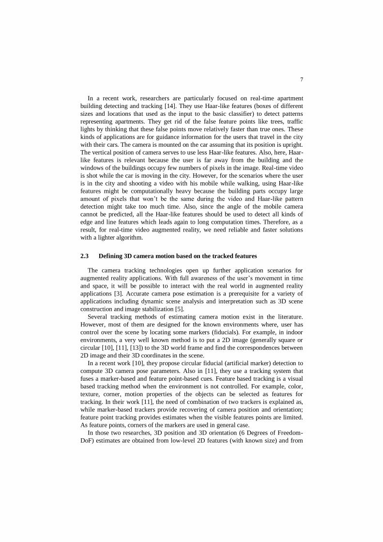
A similar application is getting closer to our purpose [17], in which, they first find

the matching line segments between aerial images. Since, the lines belong to images

of scenes containing planar surfaces (roofs); there should be a geometric relation

between corresponding lines. This geometry is called epipolar geometry. According

to epipolar constraint, there should be a point to point correspondence between

matching line segments with a fundamental matrix (Fig. 1).

Fig. 1. Image lines l and lʹ determine a line L in 3D space which is contained in family of

planes. This family of planes induces a family of homographies between the images.

They find the corresponding line in the second image by using that constraint

since epipolar geometry reduces the search space of the line segment. Then, for each

segment in the first image, they apply a correlation based algorithm for all the

segments in the second image. The algorithm is based on taking the average of the

individual correlation scores for all the pixels of the line and retain the highest score

pairs as correct matching pairs. The epipolar geometry and matched lines restrict the

possible homographies (projective transformations) between images. That means that

the correspondence of lines determines the homographies which map the line from

first image to the second one.

2.4 Vanishing Point Detection

Architectural environments consist of many parallel lines, however those lines do

not project parallel to image plane but they appear to converge to a point. Vanishing

point is a point that does not exist in real world but exist in image plane where those

lines meet.

Vanishing point concept was first used in the paintings of Renaissance Italian

painters. They tried to develop an artificial perspective in their architectural paintings

by using vanishing points. In computer vision, vanishing points are used to get the

camera geometry for calibration, depth of the scene, object dimensions, orientation of

the geometric shapes in the scene or reconstruction of the scene.

The majority of the vanishing point extraction methods use the line segments in the

image [23]. In order to detect the line segments, most of the algorithms use Hough

transform and a Gauss sphere to find the intersections whose center either located on

10

the image space or to the optical center of the camera. These methods are generally

achieved by two steps. First, they cluster the lines that possibly share the same

vanishing point which is called accumulator step. Second, they try to identify the

dominant cluster to determine vanishing points which is called search step. After

finding a vanishing point, the line segments corresponding to that vanishing point are

removed from the cluster. When there is no left dominant line cluster that exceeds a

certain threshold, the algorithm stops its search.

In order to reduce the computational time, van den Heuvel [24] used the

orthogonality information of the perpendicularity between three corresponding

orientations in the object space. In this approach, after finding the first vanishing

point, the search space for the second one is reduced. They achieve this by checking

the orthogonality of the contributed lines for each vanishing points such that the

directions of the vanishing points are orthogonal,. However, as van den Heuvel

mentioned in his paper [24] the real-time applications demand fast algorithms unlike

applications for scene reconstruction. Orthogonality check is one of the steps for the

exact estimation of the vanishing point, but also slowing down.

Rother [23] used that criteria of orthogonality and increased the computational

power by taking the midpoint of the line segments and voting the longer line

segments by giving them more weights. According to that, in the accumulator step,

the vanishing points are voted by using the relative distance between line segments

that contribute to that vanishing point, and by their lengths. Then, by using these

votes, in the search step, they check the orthogonality of the direction of vanishing

points by triangulating these three points and checking if each angle of this triangle is

less than 90°; or in two finite vanishing points case, by checking if the third vanishing

point direction is orthogonal to other two; or in one vanishing point case, if the

direction of two infinite vanishing points are orthogonal. However, even this

algorithm is faster than the previous one; it is not possible to apply it to real-time

video applications because of its computation time.

Cantoni et al. [25] compared the two Gauss-sphere approaches which differ in

parameter space and vote through the Hough transform (one operates in polar space

(ρ,θ) and the other in image space (x,y)). Here, it has been concluded that image space

approach is computationally lighter since it does not require solving a linear system

and gives higher precision results.

Besides their different extraction methods, vanishing points give significant

information about the orientation of a plane in the image [26]. For example, in the

case of a vanishing point at a far distance from the image itself, it means that the lines

are almost parallel and the viewpoint is at a perpendicular distance to that plane of

interest. This information may help to align or verify the alignment of the virtual

models correctly.

2.5 Data Fusion by Using Dempster-Shafer Theory

Data Fusion means combining the data coming from one or more sensors in a

manner that it gives the best estimation [19]. In computer vision, it is used to merge

the data coming from several sources in such a way that the knowledge of the

11

observed scene is improved. From the aspect of augmented reality applications, Data

Fusion methods are used for the combination of inertial and vision tracking systems to

satisfy the requirements of accuracy, robustness, low-jitter and ease of use [43].

Current data fusion ideas are focused on two approaches: Bayesian Theory and

Dempster-Shafer Theory. These theories are currently applied in the applications of

locating and tracking objects. In order to find the current location of the object, new

pose estimation is done by using the old state of the object. Both the Bayesian and

Dempster-Shafer approaches are based on assigning weights to the data which is used

to estimate the current state. Different than classical Bayesian Theory, Dempster-

Shafer Theory offers an alternative to traditional probabilistic theory using the

uncertainty of the state, which allows finer modelization of belief over a set of

hypothesis. As a matter of fact, a presentation of the differences of these two theories

and detailed mathematical explanation of Dempster-Shafer Theory is far beyond the

scope of this report. We will hereby explain Dempster-Shafer Theory and give

examples for its application areas.

There are three important functions in Dempster-Shafer Theory: the probability

mass function, the Belief function, and the Plausibility function [20]. Probability mass

function represents the proposition of all relevant and available evidence that supports

the claim by assigning a belief mass to that claim. Each mass is bounded by two

values called belief and plausibility. Belief is the amount that supports a given

hypothesis whereas plausibility is the amount that the hypothesis could possibly

happen up to a value. The combination of two masses is calculated by using

Dempster’s rule of combination.

According to Dempster-Shafer Theory, each sensor, Si for example, will contribute

to the probability mass function by assigning its beliefs. Therefore, according to one

of the sensor‟s observation denoted by mi, the probability of “A” to happen is

[Beliefi(A), Plausibilityi(A)].

Lower bound of the function is the sum of the evidences (Ek) that supports event

“A”: Beliefi(A) = and the upper bound is all the observations that does

not rule out the given event “A” to happen: Plausibilityi(A) =

Then, each sensor s observation, which contributes to event “A” to happen, is

combined by using Dempster-Shafer rule of combination:

The contribution of Dempster-Shafer combination algorithm to classical Bayesian

Theory is that it includes uncertainty which gives closer results to human perception.

Another contribution to Dempster-Shafer Theory is done by differentiating the

contributions of sensors in the combination algorithm [21]. The “equal trusting”

approach in the original algorithm is changed into a sensor fusion architecture in

which sensors have different accuracies which allows taking into account ignorance

estimation. The basic approach is that they use the historical performance of the

sensor to estimate the correctness rate of the sensor (whether it can make accurate

12

estimations) to decide how much the sensor‟s current estimation is trustable.

Therefore, the original changes into following, where wj is estimation correctness rate

in the history:

This model seems much more reasonable in mobile augmented reality applications

since it also takes into account the historical estimation of the sensor (and the relative

ignorance estimation) to make the current estimation. This approach might be useful

in tracking applications when there is unreliable sensor data, so that the current

estimation might be made according to previous position estimation of the object.

In outdoor-urban-environments, accurate augmented reality applications may be

used by using GPS, accelerometer, feature points and homography changes between

video frames. By defining their data as sensor information (masses) in belief function,

tracking might be more accurate by using the historical estimations when some of the

sensor data is not available or trustable.

3 Description of the work

At the beginning of the work, our main purpose was to be able to treat real-time

videos in a way that we can extract the plane information of the environment and also

the relative position of the viewer to that plane for augmented reality applications.

Plane information had a great importance since the application was due to be used in

urban environments. The scenario was that, while the user takes a video with his

smartphone, he puts some information on the buildings aligned with the planar

surface of the building. The information is supposed to be located on an intended

position like a specific window or a balcony and should keep its position on the planar

surface during the real-time video. Then, accordingly, we described the topics that we

should go through in depth.

Even if we were intending to work in unprepared outdoor environments, where it is

not possible to put markers in the scene for tracking purposes, the characteristic of

man-made environments can provide information about the scene. It is not a new idea

to use GPS and the inertial sensors of the mobile for position and orientation

measurements in an augmented reality system; however, it is also known that vision

tracking improves the robustness of the system. The initial position and orientation

information can be taken from the sensors of the mobile; however they are not

accurate to rely on totally in an augmented reality application. Nevertheless, GPS is

used to get the world coordinates, digital compass is for rotational velocity and

accelerometer is for linear acceleration of the user.

Architectural environments have parallel and orthogonal lines that can be exploited

to understand the orientation of the plane surfaces and relative position of the camera

and plane. However, it is not guarantee that the tracking of those surfaces and lines

can be accomplished in real-time. The GPS and inertial sensors of the mobile

13

provides information for each frame, separately then the tracking algorithm. However,

extraction of vision based information for each frame of the video is computationally

expensive. Therefore, we intended to use a probabilistic method for the frames that

we do not treat or cannot extract some of the information such as

line/corner/vanishing point detection or tracking.

The reason of our choice of Dempster-Shafer Data Fusion Theory is that it has

uncertainty management and the results are close to human perception. Weighted sum

of probabilities [21], as described previously, allows us to give more weight to the

more trusted sensors depending on the case. Such as, in the cases where the extraction

of the corner points are blocked by an object, the initial sensors could be given more

weight to estimate the relative position of the camera and the building; or if the

vanishing points and tracking and extraction of feature points are well established, the

inertial sensors can be given less trust since visual tracking gives more robust results.

Also, as we mentioned above, we are interested in real-time video, so the extraction

and tracking process should be fast enough. In order to achieve that, the extraction is

not done in all of the frames whereas the GPS and inertial sensors provide data

individually for each frame. Another reason of our choice of Dempster-Shafer is that

there is already a substantial amount of work that has been done on Dempster-Shafer

Theory (theory of evidence) in content based image retrieval with the contribution of

my advisor [29], [30] and that provided a valuable environment with discussions and

suggestions.

3.1 Vanishing Point Detection

Man-made environments heavily consist of regular parallel structures such as

repeating windows. When 3D edges in world coordinates transformed to 2D plane,

they carry the geometric information of the scene. Vanishing point (VP) is one of the

data that can be extracted from 2D images and can contribute to understand the

geometry of 3D world. Also, the camera intrinsic parameters can be extracted from

VPs but for the sake of simplicity, we assumed that we know the camera intrinsic

parameters of the mobile (the focal length of the lens, the size of the pixels and the

principal point coordinates in pixel coordinate system).

There are several methods for detecting vanishing points; we adopted the method

of Kalantari et al. [33], where we detect the segments, and then by using Gauss

sphere, we vote the VPs. The segments are detected by using classical method: first,

we apply Canny edge detector which convolves the image with a Gaussian filter [41].

The result is a blurred version of the image and the noise is reduced with that way.

Then, a hysteresis threshold is applied with two thresholds (upper and lower) such

that if the intensity gradient of a pixel is greater than the higher threshold, it is kept as

an edge pixel. If the intensity gradient is lower than the lower threshold, it is rejected.

For the values in between two thresholds, they are kept if there is a pixel above the

higher threshold around that pixel; otherwise they are rejected.

The distinctive characteristic of Canny edge detector is that, it tries to assemble

those candidate pixels into contours so that we can detect the line segments by using

14

Hough Transform as a next step (Fig. 2). In Canny edge detection method, the choice

of thresholds is important. If they are set too high, some of the edges cannot be

detected; on the other hand, with too low values, there will be noise remaining in the

resultant image. Although there is no generally accepted values for every image (since

intensity values may vary) Canny suggests a high to low ratio between 2:1 and 3:1

[41]. Therefore, we used TH1=15 for lower one, TH2=40 for the higher one.

For the next step, we applied Hough transform to detect the line segments from the

resultant contours (Fig. 2). There are two ways of Hough transform in general:

standard Hough Transform [32] and probabilistic Hough Transform [42].

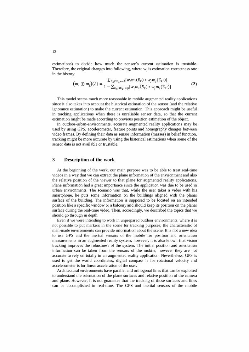
Fig. 2. On the left, Canny edge detection gives the contours of the building; on the right, Hough

transform detects the line segments that passes the canny edge

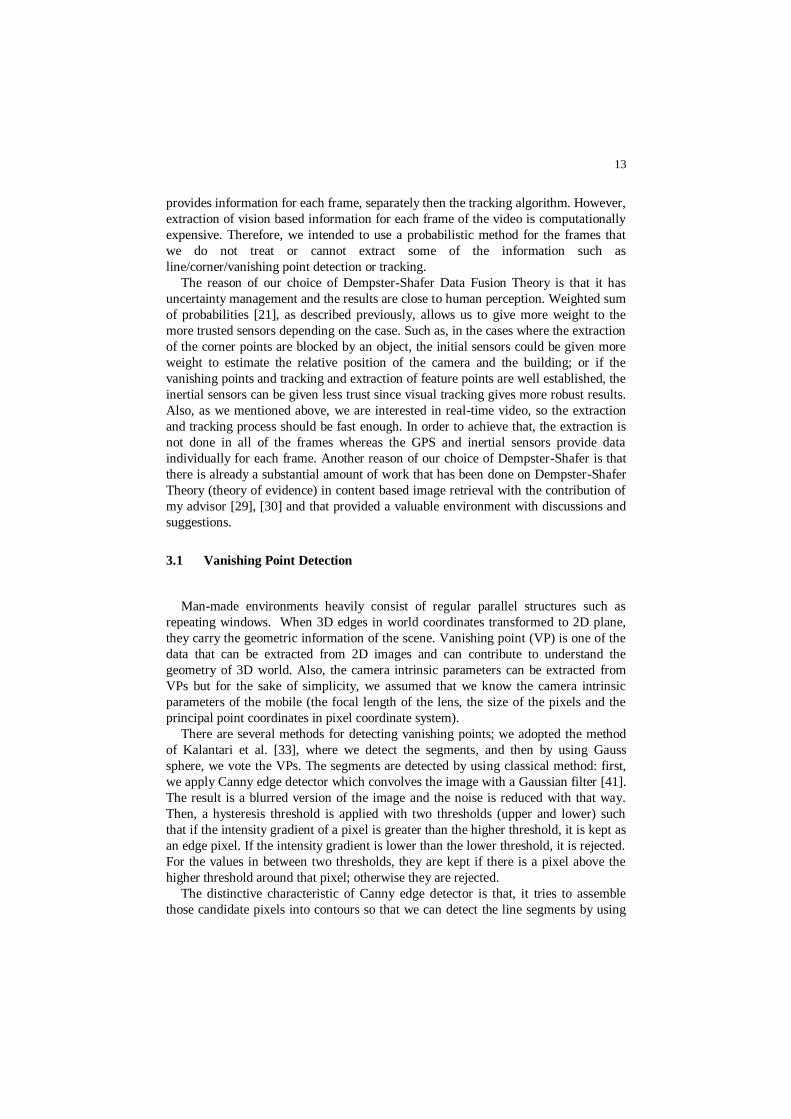
In Hough Line Transform, the lines in the image are identified by using a voting

procedure. All the lines are parameterized by the formula: . The

parameters specify a straight line by the angle θ of its normal and its distance ρ from

the origin of the image plane (Fig. 3).

Fig. 3. Parameters of a line ( )

The difference between two methods is that in the standard Hough Transform, the

algorithm performs for every point of the edges by voting them on the (ρ,θ) table (it

accumulates all the points in the (ρ,θ) plane) and then it searches through the table to

find the highest votes [32]. However, in the probabilistic method, it discards this

computational load by accumulating only a fraction of edge pixels. This approach is

known to accelerate the algorithm and reduces the computation time [42].

15

The execution time of our algorithm has as much importance as its accuracy since

we are dealing with real-time videos. Therefore, we used probabilistic Hough Line

Transform for our implementation.

One of the reasons of our choice of the method of Kalantari et al. [33] is that they

treat the image by using (x,y) image coordinates, instead of using (ρ,θ) polar

coordinates for the lines. As we declared in the State of Art, it has been proven by

Cantoni et al. [25] that image space approach is computationally lighter since it does

not require solving a linear system and gives higher precision results. The second

reason of our choice is that Kalantari et al. [33] proposed an efficient vanishing point

extraction method without any prior information of the scene. However, for the real-

time extraction purpose of our model, we made some changes on the approach.

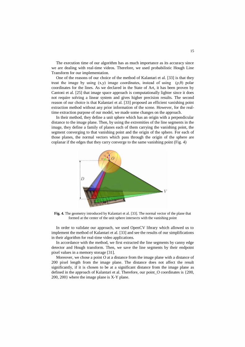
In their method, they define a unit sphere which has an origin with a perpendicular

distance to the image plane. Then, by using the extremities of the line segments in the

image, they define a family of planes each of them carrying the vanishing point, the

segment converging to that vanishing point and the origin of the sphere. For each of

those planes, the normal vectors which pass through the origin of the sphere are

coplanar if the edges that they carry converge to the same vanishing point (Fig. 4)

Fig. 4. The geometry introduced by Kalantari et al. [33]. The normal vector of the plane that

formed at the center of the unit sphere intersects with the vanishing point

In order to validate our approach, we used OpenCV library which allowed us to

implement the method of Kalantari et al. [33] and see the results of our simplifications

in their algorithm for real-time video applications.

In accordance with the method, we first extracted the line segments by canny edge

detector and Hough transform. Then, we save the line segments by their endpoint

pixel values in a memory storage [31].

Moreover, we chose a point O at a distance from the image plane with a distance of

200 pixel length from the image plane. The distance does not affect the result

significantly, if it is chosen to be at a significant distance from the image plane as

defined in the approach of Kalantari et al. Therefore, our point_O coordinates is {200,

200, 200} where the image plane is X-Y plane.

16

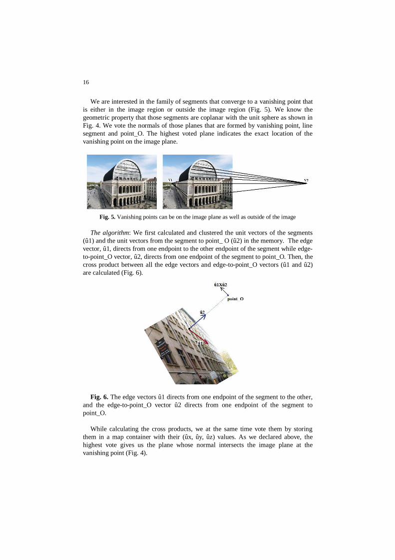
We are interested in the family of segments that converge to a vanishing point that

is either in the image region or outside the image region (Fig. 5). We know the

geometric property that those segments are coplanar with the unit sphere as shown in

Fig. 4. We vote the normals of those planes that are formed by vanishing point, line

segment and point_O. The highest voted plane indicates the exact location of the

vanishing point on the image plane.

Fig. 5. Vanishing points can be on the image plane as well as outside of the image

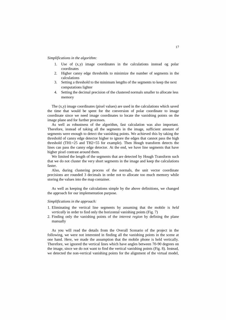
The algorithm: We first calculated and clustered the unit vectors of the segments

(û1) and the unit vectors from the segment to point_ O (û2) in the memory. The edge

vector, û1, directs from one endpoint to the other endpoint of the segment while edge-

to-point_O vector, û2, directs from one endpoint of the segment to point_O. Then, the

cross product between all the edge vectors and edge-to-point_O vectors (û1 and û2)

are calculated (Fig. 6).

Fig. 6. The edge vectors û1 directs from one endpoint of the segment to the other,

and the edge-to-point_O vector û2 directs from one endpoint of the segment to

point_O.

While calculating the cross products, we at the same time vote them by storing

them in a map container with their (ûx, ûy, ûz) values. As we declared above, the

highest vote gives us the plane whose normal intersects the image plane at the

vanishing point (Fig. 4).

17

Simplifications in the algorithm:

1. Use of (x,y) image coordinates in the calculations instead og polar

coordinates

2. Higher canny edge thresholds to minimize the number of segments in the

calculations

3. Setting a threshold to the minimum lengths of the segments to keep the next

computations lighter

4. Setting the decimal precision of the clustered normals smaller to allocate less

memory

The (x,y) image coordinates (pixel values) are used in the calculations which saved

the time that would be spent for the conversion of polar coordinate to image

coordinate since we need image coordinates to locate the vanishing points on the

image plane and for further processes.

As well as robustness of the algorithm, fast calculation was also important.

Therefore, instead of taking all the segments in the image, sufficient amount of

segments were enough to detect the vanishing points. We achieved this by taking the

threshold of canny edge detector higher to ignore the edges that cannot pass the high

threshold (TH1=25 and TH2=55 for example). Then Hough transform detects the

lines can pass the canny edge detector. At the end, we have line segments that have

higher pixel contrast around them.

We limited the length of the segments that are detected by Hough Transform such

that we do not cluster the very short segments in the image and keep the calculations

faster.

Also, during clustering process of the normals, the unit vector coordinate

precisions are rounded 3 decimals in order not to allocate too much memory while

storing the values into the map container.

As well as keeping the calculations simple by the above definitions, we changed

the approach for our implementation purpose.

Simplifications in the approach:

1. Eliminating the vertical line segments by assuming that the mobile is held

vertically in order to find only the horizontal vanishing points (Fig. 7)

2. Finding only the vanishing points of the interest region by defining the plane

manually

As you will read the details from the Overall Scenario of the project in the

following, we were not interested in finding all the vanishing points in the scene at

one hand. Here, we made the assumption that the mobile phone is held vertically.

Therefore, we ignored the vertical lines which have angles between 70-90 degrees on

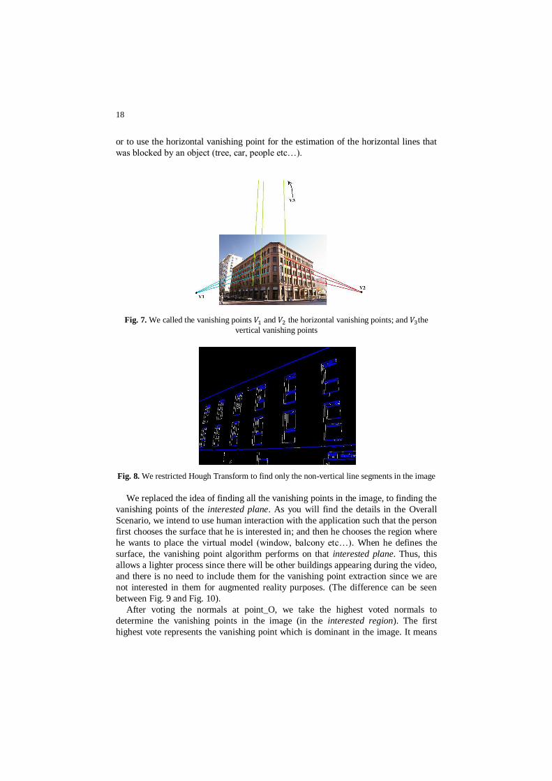
the image, since we do not want to find the vertical vanishing points (Fig. 8). Instead,

we detected the non-vertical vanishing points for the alignment of the virtual model,

18

or to use the horizontal vanishing point for the estimation of the horizontal lines that

was blocked by an object (tree, car, people etc…).

Fig. 7. We called the vanishing points and the horizontal vanishing points; and the

vertical vanishing points

Fig. 8. We restricted Hough Transform to find only the non-vertical line segments in the image

We replaced the idea of finding all the vanishing points in the image, to finding the

vanishing points of the interested plane. As you will find the details in the Overall

Scenario, we intend to use human interaction with the application such that the person

first chooses the surface that he is interested in; and then he chooses the region where

he wants to place the virtual model (window, balcony etc…). When he defines the

surface, the vanishing point algorithm performs on that interested plane. Thus, this

allows a lighter process since there will be other buildings appearing during the video,

and there is no need to include them for the vanishing point extraction since we are

not interested in them for augmented reality purposes. (The difference can be seen

between Fig. 9 and Fig. 10).

After voting the normals at point_O, we take the highest voted normals to

determine the vanishing points in the image (in the interested region). The first

highest vote represents the vanishing point which is dominant in the image. It means

19

that most of the segments in the image contribute to that vanishing point. After

finding that normal, we intersect it with the image plane and find the vanishing point

coordinates.

Fig. 9. All the horizontal vanishing points are found in the image in one iteration

Fig. 10. The region of interest is defined manually

Fig. 11. Two example images where we define the interest plane by choosing the plane

manually (by mouse)

Experimental Results: We are able to find more than one vanishing point in the

image by single iteration (Fig. 9). For our implementation purpose, we are not

extracting the vertical vanishing points. Therefore, we used the non-vertical lines to

extract the vanishing points. However, we are not interested to extract them through

20

the entire image. Therefore, we restricted our algorithm to finding the vanishing

points on the interested surfaces where we want to track some of its elements

(balcony, window etc…). You will see our resulting images on Fig. 10 and Fig. 11

where we define the interested surface plane manually. Vertical line elimination from

the calculations has increased the iteration time 10.7%. Moreover, by setting the

minimum length of a line segment that will be returned, the computation time

improves 8%.

3.2 Corner Detection and Tracking

In our implementation, a reliable tracking system is one of the most important

components for the accuracy. As we discussed in the state of art of this report, the

performance of the tracking algorithm is important since we intend to use it in real-

time application. In order to keep the calculations less, we used the property of video

frames in which the feature locations doesn‟t move significantly in the sequential

frames. Therefore, we restricted the search region of the feature points in the next

frame, instead of tracking all the features in the image. We called that window

―search window‖, whose dimensions are calculated by the interested window on the

building. First, the building window is chosen by the user on which he wants to locate

the virtual model, and then features are calculated. For the next frames, we predict the

expected location of the search window and track the features in that region. In the

cases of obstacle in the scene, where we cannot detect some of the features or miss all

of them, we intend to keep the virtual model and the search region in the correct

location by using Dempster-Shafer model. Then, we try to detect the building window

and features in the next frames, where there is no obstacle anymore, by using

Dempster-Shafer Theory.

A similar idea for real-time application is proposed by Park et al. [34]. In this

approach, once the feature positions are detected in the next frame, by using search

window, the current feature states are kept in a history buffer. We use that approach in

search window prediction by using inertial sensors and Dempster-Shafer Theory.

We should choose the features such that they are scale, translation and rotation

invariant. Features can be classified as region-based, edge-based and point-based

features. As Tissainayagam and Suter compared them for video tracking applications

in their research [35], since there are not many differences between consecutive

frames, tracking regions (blobs) is not easy in videos. Also, as it is referred in this

study, edge tracking lead to inaccuracies since during motion, the edge segments tend

to split and merge and also because only the perpendicular flow of the edge can be

tracked. However, point features are distinctive elements that can be located

accurately in successive images.

Corners refer to the points that have two dimensional intensity change and they

give more reliable results than edge tracking since flow changes are fully recoverable.

Since our application is based on tracking features on building structures where there

are many parallel lines that intersect, we chose corner points to track instead of edges

since tracking process is more reliable [35] and corner points are invariant to scale

[37]. As well as deciding the tracking method, choosing the convenient corner

21

tracking method is important. We did not focus ourselves on the point feature tracking

methods SIFT or SURF since they are heavy for real time applications as we declared

in the State of Art. For this reason, we consulted to framework of Tissainayagam and

Suter [35] where they assess four different corner tracking methods (Kitchen-

Rosenfield, Harris, KLT and Smith) for real-time video applications. After

performance measure analysis, the results show that the Harris and KLT corner

detection methods provide best quality corners and tracking performance. Harris

corner detector based on a smoothing function as a part of its formulation (intensity

gradients are calculated on a Gaussian smoothed region by 3x3 image pixel patch)

which makes it more robust to noise. It has been proven that it is highly reliable in

finding L-junctions [36] which suits to our project since many corner points on

buildings images are L-junctions. Therefore, we chose Harris corner detection method

for our implementation.

The performance of finding and matching corners in a video stream depends on if

the points are temporarily stable and can be detected in every frame and if their

position is close enough to the previous frame. As we declared in the description of

the work, we intend to skip a reasonable number of frames for the tracking since

extraction of vision based information for each frame might be computationally

expensive. However, the number of skipped frames should be chosen such that the

tracking will not fail. For the frames that we skipped and did not track the points we

use a probabilistic method with inertial sensors to determine the virtual model

position that is explained in the following.

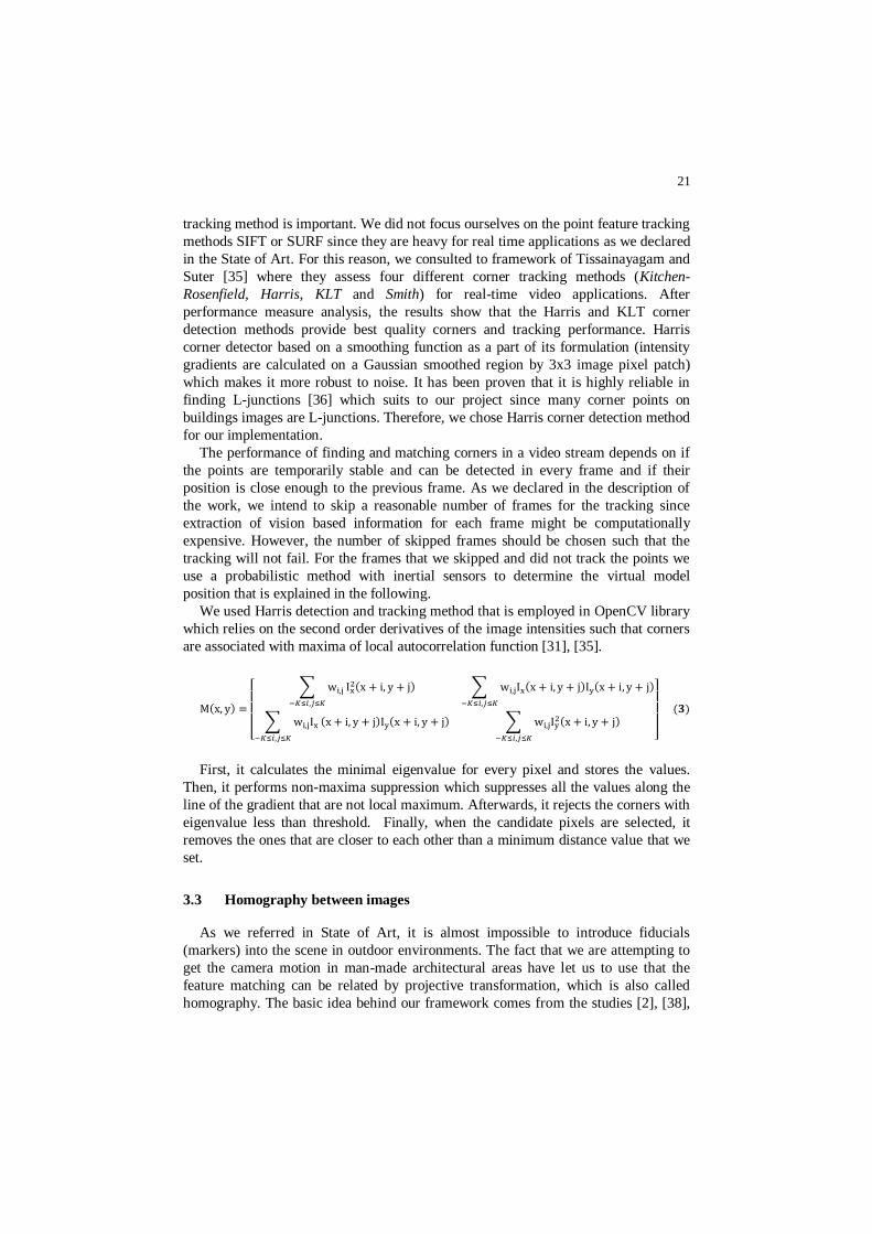
We used Harris detection and tracking method that is employed in OpenCV library

which relies on the second order derivatives of the image intensities such that corners

are associated with maxima of local autocorrelation function [31], [35].

First, it calculates the minimal eigenvalue for every pixel and stores the values.

Then, it performs non-maxima suppression which suppresses all the values along the

line of the gradient that are not local maximum. Afterwards, it rejects the corners with

eigenvalue less than threshold. Finally, when the candidate pixels are selected, it

removes the ones that are closer to each other than a minimum distance value that we

set.

3.3 Homography between images

As we referred in State of Art, it is almost impossible to introduce fiducials

(markers) into the scene in outdoor environments. The fact that we are attempting to

get the camera motion in man-made architectural areas have let us to use that the

feature matching can be related by projective transformation, which is also called

homography. The basic idea behind our framework comes from the studies [2], [38],

22

[39] and [40] where they described the geometry understandably. We used this

concept in understanding the camera movement in the scene and estimating the next

movement by using Dempster-Shafer model. The feature displacement between two

images depends both on the camera motion and the camera distance from the planar

surface. Homography helps us to understand this movement in the scene.

We used „points‟ for feature matching to extract the homography, (instead of

segments or pixel intensities etc…) since we already extract them for tracking.

Homography (plane projective transformation) is a mapping of points from one image

to another and describes the rotational and translational movement. Under perspective

transformation, the points are related by: where X is the world coordinates

and x is the image coordinates and H is the plane projective matrix (homography)

between world points and image points described by where K is intrinsic

camera matrix, R is the rotation matrix and t is the translation vector [40]. Intrinsic

camera matrix K contains the intrinsic parameters of camera:

where f is focal length, and are the horizontal and vertical pixel sizes on the

image plane and is the projection of the camera center (principal point) on

the image plane. The intrinsic parameters of the mobile camera are assumed to be

known for our framework in order to focus ourselves on homography extraction and

camera motion estimation. The describes the motion of the camera:

where R is a 3x3 rotation matrix and t is a 3x1 translation vector. Therefore H is a

3x3 matrix that maps coordinate x in one image to in another.

Although it contains nine elements, there are only eight independent elements.

Therefore, a homography can be described by using four point correspondences

between two images (Fig. 12) since each correspondence generates two linear

equations [2], [38]. However more points will define more accurate results. As we

described above in Corner Detection and Tracking part, we used a search window in

order to extract and track the feature points (corners). For homography calculations,

we are using the same search window by estimating its position for the following

frames and extracting the matching points. Four corner points of the interested

window on the building surface can be used for tracking and the calculation of the

homography. However, since our search window is small with respect to the image, it

will not change the computation time if we define higher points than „4‟. Therefore,

we defined the maximum tracking points as „10‟. Also, in order to get a good spread

23

of points in the search window, we kept the points which are closer to each other less

than five pixels. The best selection of corner points will be the corners of the

interested window of the building surface, however there will be cases when some of

the corners could not be tracked in some frames.

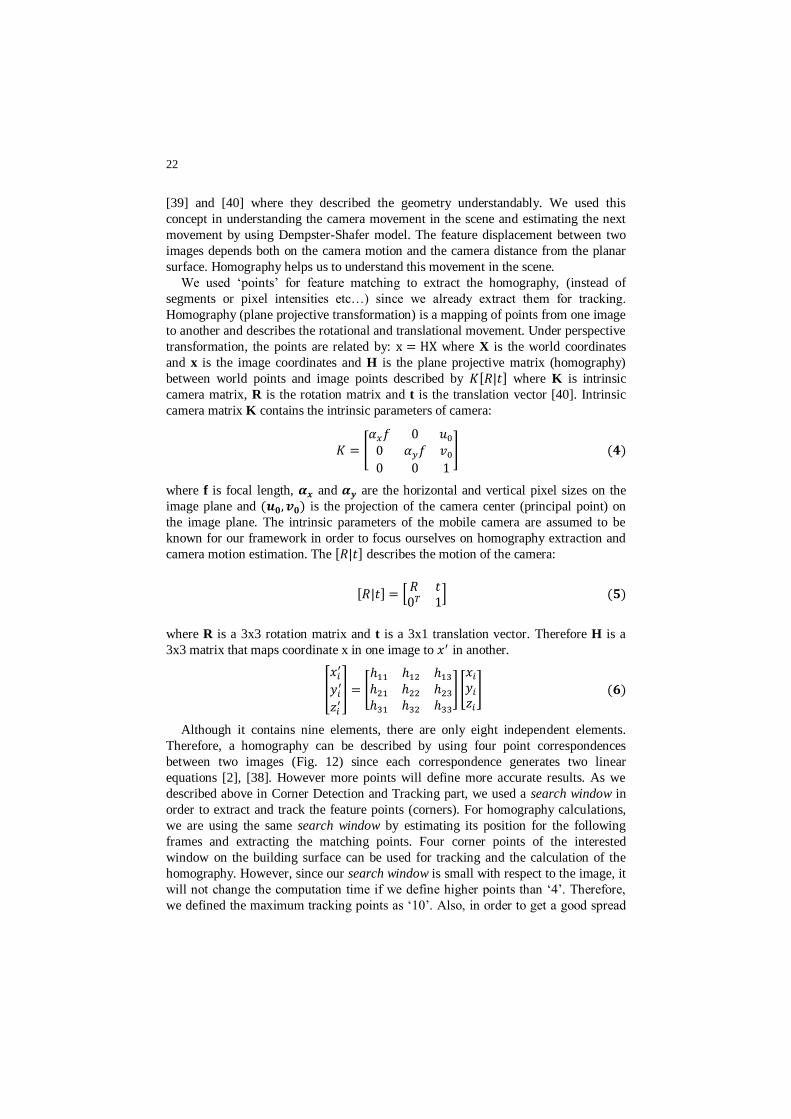
Fig. 12. Homography defines a map between a point in the first image and its

correspondence in image i

Overview of the homography calculation:

Detect the corner points in the first search window of the first frame.

Detect the corner points for the second frame assuming that the search

window remains the same.

Track the corners by choosing the candidate point in the next frame which

maximizes the cross-correlation

If there are at least 4 corresponding points in the search window of two

images, then calculate the homography between these images.

3.3.1 Computation of

If and are two image coordinates in the consecutive

frames belonging to the same 3D point in world coordinates, their coordinates can be

related by:

where λ is the homogeneous scale factor [40]. By cross multiplication, we obtain the

linear system of two equations:

24

such that given four correspondences, we can solve the equations [38], [40].

3.4 Inner sensors contribution

For the initial frames of the video, we are not using the inner sensors of the mobile

to estimate the search window position since we do not know the relative distance

between the camera and the plane. For example, if the camera is far away from the

building surface, the same angular movement will correspond to a big change in

search window position, and a small change if the camera is closer to the plane.

Therefore, the estimation will not be accurate by only using inner sensors; since we

do not know how many pixels we should slide the search window. However, after a

sufficient amount of homography calculation between frames, we can associate the

sensor data with search window.

The inner sensor data is obtained for each frame as a characteristic of mobile

phones. We can save the search window movements in a history buffer and by

comparing them with the sensor data; we can define the correspondent movement of

the search window with respect to the sensor data.

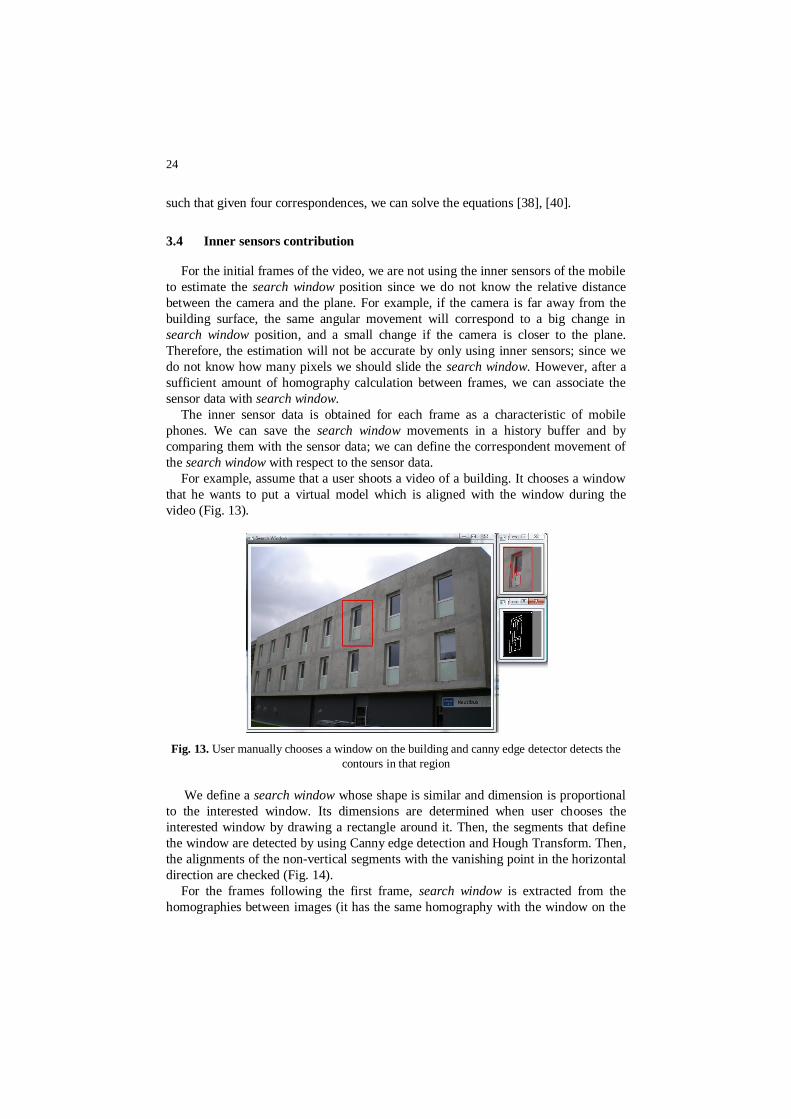
For example, assume that a user shoots a video of a building. It chooses a window

that he wants to put a virtual model which is aligned with the window during the

video (Fig. 13).

Fig. 13. User manually chooses a window on the building and canny edge detector detects the

contours in that region

We define a search window whose shape is similar and dimension is proportional

to the interested window. Its dimensions are determined when user chooses the

interested window by drawing a rectangle around it. Then, the segments that define

the window are detected by using Canny edge detection and Hough Transform. Then,

the alignments of the non-vertical segments with the vanishing point in the horizontal

direction are checked (Fig. 14).

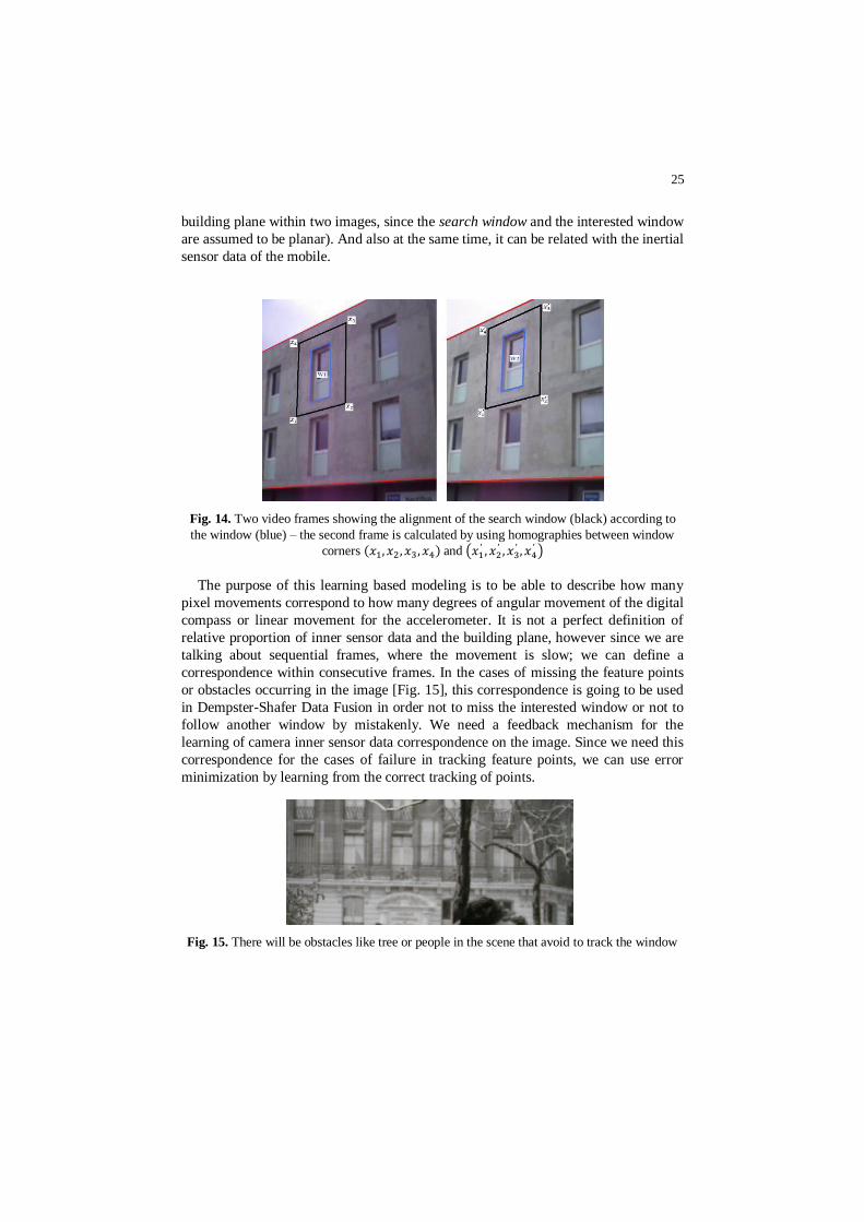
For the frames following the first frame, search window is extracted from the

homographies between images (it has the same homography with the window on the

25

building plane within two images, since the search window and the interested window

are assumed to be planar). And also at the same time, it can be related with the inertial

sensor data of the mobile.

Fig. 14. Two video frames showing the alignment of the search window (black) according to

the window (blue) – the second frame is calculated by using homographies between window

corners and

The purpose of this learning based modeling is to be able to describe how many

pixel movements correspond to how many degrees of angular movement of the digital

compass or linear movement for the accelerometer. It is not a perfect definition of

relative proportion of inner sensor data and the building plane, however since we are

talking about sequential frames, where the movement is slow; we can define a

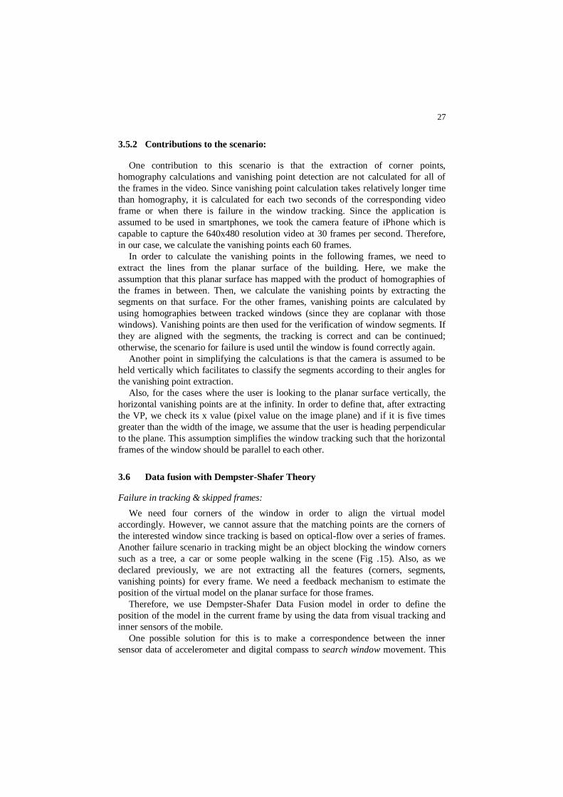
correspondence within consecutive frames. In the cases of missing the feature points

or obstacles occurring in the image [Fig. 15], this correspondence is going to be used

in Dempster-Shafer Data Fusion in order not to miss the interested window or not to

follow another window by mistakenly. We need a feedback mechanism for the

learning of camera inner sensor data correspondence on the image. Since we need this

correspondence for the cases of failure in tracking feature points, we can use error

minimization by learning from the correct tracking of points.

Fig. 15. There will be obstacles like tree or people in the scene that avoid to track the window

26

3.5 Overall Scenario

3.5.1 Algorithm Summary

Here we summarized our algorithm in two possible scenarios, one is when the

tracking achieved successfully, second is when there is failure in tracking. The second

scenario is where we use a probabilistic approach to get back the tracked window, or

not to lose it in the cases of obstacle.

For successful tracking:

1. Manually indicate the planar surface of the building

2. Find the non-vertical segments on that region and the vanishing point from that

segments

3. Choose the window where we want to hold the virtual model by manually

indicating a rectangular region on that surface of the building

4. Find the segments in that region

5. Find the largest quadrilateral region to define the window by checking the

alignment of non-vertical segments with the vanishing points

6. Align the rectangular region to a quadrilateral region proportional to the window

(Fig. 14)

7. Find maximum 10 corner points in the quadrilateral region in frame 0

8. Find maximum 10 corner points in the next frame (frame 1)

9. Match those points with the ones in the first frame

10. Check if 4 corner points of the interested window are matched

o If they are matched use these 4 points to define homography

o Otherwise use the matched ones from those corners and sum up to 4

by choosing the other matching points randomly

11. Define the homography between frame i to i+1 by using 4 corresponding

points

12. Define the new position of the vanishing point by multiplying it with the

homography matrix

13. Define the positions of the corner points in frame 1 by using matched corners

and homography for the not-matched ones

14. Check the alignments of the segments with the window in frame 1 and the

defined vanishing point by checking the corner points (if not, failure in tracking)

15. Define the new quadrilateral “search region” for image i+1 by multiplying

with the homography

16. Save the direction of movement of quadrilateral “search region” pixel wise in

the history buffer with the acceleration and digital compass data

17. Use this quadrilateral “search region” for tracking the corners in i+2 frame

18. Repeat the algorithm from 7 to 17 by using the consecutive frames.

27

3.5.2 Contributions to the scenario:

One contribution to this scenario is that the extraction of corner points,

homography calculations and vanishing point detection are not calculated for all of

the frames in the video. Since vanishing point calculation takes relatively longer time

than homography, it is calculated for each two seconds of the corresponding video

frame or when there is failure in the window tracking. Since the application is

assumed to be used in smartphones, we took the camera feature of iPhone which is

capable to capture the 640x480 resolution video at 30 frames per second. Therefore,

in our case, we calculate the vanishing points each 60 frames.

In order to calculate the vanishing points in the following frames, we need to

extract the lines from the planar surface of the building. Here, we make the

assumption that this planar surface has mapped with the product of homographies of

the frames in between. Then, we calculate the vanishing points by extracting the

segments on that surface. For the other frames, vanishing points are calculated by

using homographies between tracked windows (since they are coplanar with those

windows). Vanishing points are then used for the verification of window segments. If

they are aligned with the segments, the tracking is correct and can be continued;

otherwise, the scenario for failure is used until the window is found correctly again.

Another point in simplifying the calculations is that the camera is assumed to be

held vertically which facilitates to classify the segments according to their angles for

the vanishing point extraction.

Also, for the cases where the user is looking to the planar surface vertically, the

horizontal vanishing points are at the infinity. In order to define that, after extracting

the VP, we check its x value (pixel value on the image plane) and if it is five times

greater than the width of the image, we assume that the user is heading perpendicular

to the plane. This assumption simplifies the window tracking such that the horizontal

frames of the window should be parallel to each other.

3.6 Data fusion with Dempster-Shafer Theory

Failure in tracking & skipped frames:

We need four corners of the window in order to align the virtual model

accordingly. However, we cannot assure that the matching points are the corners of

the interested window since tracking is based on optical-flow over a series of frames.

Another failure scenario in tracking might be an object blocking the window corners

such as a tree, a car or some people walking in the scene (Fig .15). Also, as we

declared previously, we are not extracting all the features (corners, segments,

vanishing points) for every frame. We need a feedback mechanism to estimate the

position of the virtual model on the planar surface for those frames.

Therefore, we use Dempster-Shafer Data Fusion model in order to define the

position of the model in the current frame by using the data from visual tracking and

inner sensors of the mobile.

One possible solution for this is to make a correspondence between the inner

sensor data of accelerometer and digital compass to search window movement. This

28

correspondence can be used in the history buffer and for the cases of failure in

tracking; we can estimate the location of the search window until we get back to

successful tracking again. For example, imagine that a user makes a rotational

movements and there is a tree that window could not tracked. Then the

correspondence in the history buffer might be used to estimate how many degree of

angular movement of the mobile corresponds to how many pixel of movement of

search window in the image. However, it should not be forgotten that the nearer

correspondence in the history buffer should be used since the user might have

changed his position in the much previous frames and also the angle to the planar

surface might have been changed significantly.

However, for the initial frames (5-10 frames), it is expected to be that the window

is tracked correctly so that there is enough data to make this correspondence. If the

frames are not the initial frames of the video, (after 5 frames), we start to use the

estimation model, that we describe in the following, for the search window by using

accelerometer and digital compass.

To be more precise, we are assigning adaptable weights to the sensor data that

comes from the gyroscope and accelerometer of the smartphone. The weights are

assigned in such a way that when the vision tracking method is not reliable, we should

not miss the tracked features on the building surface. Therefore, for gyroscope

example, we keep the pixel wise movement of the search window with respect to

angular movement of the gyroscope in a history buffer (1 degree of angular

movement in vertical direction corresponds to 5 pixel slide of the search window for

example). This data helps us to estimate to make the correspondence between an

inertial sensor data and the distance to the plane as we explained above. Then by

using this data, if we miss some of the corner points of the window (Fig. 15), or the

detected segment cannot be aligned with the vanishing point, then we assign higher

belief value to the inertial sensor data until we recover the tracked features and

aligned segments with respect to vanishing points. We used the idea in [34] for the

basic pseudo-code of the algorithm:

o Step 1 (Initialization)

o Capture and load the first frame

o Extract 10 feature points from the first frame

o Track them in the following frame

o Save the sensor data with the tracking data to history buffer

o If the corner points could not tracked

increase the weight of the sensors for the prediction step

decrease the weight of the vision tracking (homographies, VP alignment)

o Step 2 (Prediction):

o Capture and load the next frame.

o Predict the feature state by using the correspondence from the recent history

o Set the search window location according to the prediction

o Loop in step 2 until the feature points are recovered (more trust to sensor data)

o Step 3 (Tracking features):

o Increase the weights of the vision tracking data

o Go to Step 1

29

This part of the implementation requires specific programming methods and a deeper,

oriented study with mobile sensor data treatment. We examined the use of the method

in several articles [8], [12], [13] and [21], and proposed a pseudo-code above by

adapting it to our implementation.

4 Conclusion

In this report, we proposed a hybrid approach for real-time augmented reality in

urban environments. We tried to handle the problem in several aspects. The difference

of our proposition from previous works is the utilization of the probabilistic fusion of

the vision-based data with the sensor-based data. While doing this data fusion, we

used the history of the feature locations in order to estimate the new locations for the

next frames which let us to reduce our search space and computation time. For the

extraction of the vision-based tracking information, we are using the properties of

man-made architectures such as parallel lines and planar surfaces.

In order to validate several aspects of our methodology, we employed OpenCV

computer vision library which allowed us to see that our approach is computationally

lighter.

The main limitation of our approach is that we assume that the window frames are

composed of parallel lines without including the possibility that they could rely on

other architectural shapes.

In the continuation of our study, the quantitative analysis of the sensitiveness of

sensor-based tracking could be done with a smartphone. Also, the possibility of

having distinctive architectures (artistic structures) could be studied. Another

possibility is that the approach could be merged with a touristic aspect, such that the

known historical buildings could be treated with their known distinctive design

properties recovered from the database saved images in the with some images saved

in the database (irregular window frames, gothic style buildings could be used as an

example).

Acknowledgements. I would first like to express my sincere appreciation to my

advisor, Prof. Bruno TELLEZ, for his wise guidance, witty suggestions and

interesting discussions during my internship. Without his enthusiasm, inspiration and

efforts to make things clear and understandable, this report would not have been

completed.

I also wish to thank my family for their emotional support and trust in me

throughout my life and for leaving me free for all my decisions.

My special thanks to Jun-Young BAE for his constant kindness and cheerful

support in every step of my studies. Without him and his generous gift (the coffee

machine) that accompanied me during my sleepless nights, the preparation of this

thesis would have been a lot more difficult.

I also gratefully salute my undergraduate faculty (EEE) members and university

(METU) for enriching me in such a way that I found enough courage and knowledge

to pursue a master in Image and Graphics.

30

Thanks are due also to the professors, my colleagues and the friendly environments

of interns in the LIRIS research laboratory.

References

[1] I.M. Zendjebil, F. Ababsa, J. Didier, J. Vairon, L. Frauciel, M. Hachet, P. Guitton, R.

Delmont. « Réalité Augmentée en extérieur: Enjeux et Etat de l‟Art ». 2èmes journées de

l'AFRV, Marseille, France, 25-26 Octobre, 2007

[2] S. Prince, K. Xu, A. Cheok. « Augmented reality camera tracking with homographies ».

IEEE Comput. Graph. Appl. 22 (6) (2002) 39–45. 2002

[3] C. Woodward, M. Hakkarainen, K. Rainio. « Mobile Augmented Reality for Building and

Construction » VTT Technical Research Centre of Finland. Mobile AR Summit MWC 2010.

February 2010

[4] M. Hakkarainen, C. Woodward, K. Rainio. « Software Architecture for Mobile Mixed

Reality and 4D BIM Interaction » in Proc. 25th CIB W78 Conference, 1-3 Oct 2009,

Istanbul, Turkey, 8, pp. 517-524. 2009

[5] B. Jiang, S. You U. Neumann. « Camera Tracking for Augmented Reality Media » IEEE

International Conference on Multimedia and Expo (III), pages 1637—1640. 2000.

[6] B. Reitinger, C. Zach, D. Schmalstieg « Augmented Reality Scouting for Interactive 3D

Reconstruction « in Proceedings of IEEE Virtua Reality, pages 219-222. 2007

[7] N. Snavely, S. M. Seitz, R. Szeliski « Photo Tourism: Exploring Photo Collections in 3D »

ACM Transactions on Graphics. August 2006

[8] G. Schall, D. Wagner, G. Reitmayr, E. Taichmann, M. Wieser, D. Schmalstieg, B.

Hofmann-Wellenhof. « Global Pose Estimation using Multi-Sensor Fusion for Outdoor

Augmented Reality » Proceedings of the 2009 8th IEEE International Symposium on Mixed

and Augmented Reality Pages: 153-162. 2009

[9] P. Honkamaa, S. Siltanen, J. Jäppinen, C. Woodward, O. Korkalo, « Interactive outdoor

mobile augmentation using markerless tracking and GPS » VTT Technical Research Centre

of Finland. Proc. Virtual Reality International Conference (VRIC), Laval, France, April

2007, pp. 285-288. 2007

[10] F. Ababsa, M. Mallem. « A Robust Circular Fiducial Detection Technique and Real Time

3D Camera Tracking » Journal of Multimedia Vol. 3, No. 4, October 2008. 2008

[11] D. Marimon, T. Ebrahimi « Combination of videobased camera trackers using a

dynamically adapted particle filter » Proc. 2nd International Conference on Computer

Vision Theory and Applications (VISAPP07), p. 363-370. 2007

[12] S. You, U. Neumann, R. Azuma « Hybrid inertial and vision tracking for augmented

reality registration » In IEEE Virtual Reality (VR), pages 260–267. 1999

[13] S. You, U. Neumann. « Fusion of Vision and Gyro Tracking for Robust Augmented

Reality Registration » In IEEE Virtual Reality (VR), page 71. 2001

[14] Y. Hu, D. S. Jang, J. H. Park, S. I. Cho, C. W. Lee « Real-Time Apartment Building

Detection and Tracking with AdaBoost Procedure and Motion-Adjusted Tracker » ETRI

Journal, vol.30, no.2, Apr. 2008, pp.338-340. 2008

[15] D. Nistér. « An efficient solution to the five-point relative pose problem » IEEE

Transactions on Pattern Analysis and Machine Intelligence (PAMI), 26(6):756-770. June

2004

[16] J. Wither, S. DiVerdi, T. Höllerer « Using aerial photographs for improved mobile AR

annotation » Proceedings of the 5th IEEE and ACM International Symposium on Mixed and

Augmented Reality, pages: 159-162. 2006

31

[17] C. Scmid, A. Zisserman. « Automatic Line Matching across Views » Proceedings of the

1997 Conference on Computer Vision and Pattern Recognition, p.666. 1997

[18] C. Harris, C. Stennett. « RAPID - a video rate object tracker » Proc. 1st British Machine

Vision Conference, pp. 73-77. Sep. 1990

[19] D. Koks, S. Challa. « An Introduction to Bayesian and Dempster-Shafer Data Fusion »

Australian Government Department of Defense. 2003

[20] K. Sentz, S. Ferson. « Combination of Evidence in Dempster-Shafer Theory » National

Laboratories SAND 2002-0835. 2002

[21] H. Wu, M. Siegel, R. Stiefelhagen, J. Yang. « Sensor Fusion Using Dempster-Shafer

Theory » IEEE International Measurement Technology Conference (IMTC). 2002

[22] A. Yilmaz, O. Javed, M. Shah. « Object tracking: A survey » ACM Comput. Surv. 38, 4,

Article 13, 45 pages. Dec. 2006

[23] C. Rother. « A new approach for vanishing point detection in architectural environments »

11th British Machine Vision Conference, Bristol, UK, pp 382-291. 2000

[24] F. A. van den Heuvel. « Vanishing point detection for architectural photogrammetry »

International Archives of Photogrammetry and Remote Sensing, Vol. XXXII part 5, pp. 652-

659. 1998

[25] V. Cantoni, L. Lombardi, M. Porta, N. Sicard. « Vanishing Point Detection:

Representation Analysis and New Approaches » Proceedings of ICIAP 2001, pp. 90-94.

2001.

[26] P. David. « Detecting planar surfaces in outdoor urban environments » (ebook) Adelphi,

MD, Army Research Laboratory. 2008

[27] D.G. Lowe. « Distinctive image features from scale-invariant keypoints » International

Journal of Computer Vision, 60(2):91-110. 2004

[28] H. Bay, T. Tuytelaars, L. Van Gool. « SURF: Speeded up robust features » ECCV. 2006

[29] S. Bres, B. Tellez. « Localisation and augmented reality for mobile applications in cultural

heritage » 3rd International Workshop 3D ARCH 2009. 25-28 February, 2009

[30] N. Zlatoff « Indexation d'images 2D Vers une reconnaissance d'objets multicritères »

Thèse préparé au sein du laboratoire LIRIS sous la direction de Atilla Baskurt et Bruno

Tellez, soutenu le 12 juillet 2006

[31] BOOK : G. Bradski, A. Kaehler « Learning OpenCV: Computer Vision with the OpenCV

Library » Publisher : O’Reilly Media, Released. September 2008

[32] R. O. Duda, P. E. Hart. « Use of the Hough Transformation to Detect Lines and Curves in

Pictures » Communication of the ACM, 15(1), 11-15. 1972

[33] M. Kalantari, F. Jung, N. Paparoditis, J.P. Guédon. « Robust and Automatic Vanishing

Points Detection with their Uncertainties from a Single Uncalibrated Image, by Planes

Extraction on the Unit Sphere » International Archives of Photogrammetry, Remote Sensing

and Spatial Information Sciences. Vol. 37 (Part 3A), pp.203-208, Beijing, China. July 2008

[34] J.-S. Park, J.-H. Yoon, C. Kim. « Stable 2D Feature Tracking for Long Video Sequences »

International Journal of Signal Processing, Image Processing and Pattern Recognition,

Vol.1, No.1, pp.39-46. Dec. 2008

[35] P. Tissainayagam, D. Suter. « Assessing the Performance of Corner Detectors for Point

Feature Tracking Applications » Image and Vision Computing, 22: 663-679. 2004

[36] J. A. Noble. « Finding Corners » Image and Vision Computing, Vol.6(2), pp.121-128. 1988

[37] F. Ababsa, M. Mallem. « Robust Camera Pose Estimation Using 2D Fiducials Tracking

for Real-Time Augmented Reality Systems » VRCAI 2004 pp. 431-435, Nanyang

(Singapore). December 2004

[38] J. Košecká, W. Zhang. « Extraction, matching and pose recovery based on dominant

rectangular structures » CVIU, 100(3):174–293. 2005

32

[39] R. Hartley, A. Zisserman « Multiple View Geometry» CVPR. June 1999

[40] G. Simon, A. W. Fitzgibbon, A. Zisserman. « Markerless tracking using planar structures

in the scene » ISAR. 2000

[41] J. Canny, « A computational approach to edge detection » IEEE Transactions on Pattern

Analysis and Machine Intelligence 8: 679–714. 1986

[42] N. Kiryati, Y. Eldar, A. M. Bruckshtein, « A probabilistic Hough transform » Pattern

Recognition 24: 303–316. 1991

[43] W. T. Fong, S.K. Ong, A. Y. C. Nee « Computer Vision Centric Hybrid Tracking for

Augmented Reality in Outdoor Urban Environments » VRCAI 2009: 185-190. 2009