ORI GIN AL PA PER

Hurricane winds over the North Atlantic: spatial analysisand sensitivity to ocean temperature

Jill C. Trepanier

Received: 25 July 2013 / Accepted: 26 November 2013 / Published online: 15 December 2013� Springer Science+Business Media Dordrecht 2013

Abstract Hurricanes pose serious threats to people and infrastructure along the United

States Gulf and Atlantic coasts. The risk of the strongest hurricane winds over the North

Atlantic basin is analyzed using a statistical model from extreme value theory and a

tessellation of the domain. The spatial variation in model parameters is shown, and an

estimate of the limiting strength of hurricanes at locations across the basin is provided.

Quantitative analysis of the variation is done using a geographically weighted regression

with regional sea surface temperature as a covariate. It is found that as sea surface tem-

peratures increase, the expected hurricane wind speed for a given return period also

increases.

Keywords Hurricane � Risk � Extreme value � Tessellation

1 Introduction

Hurricanes are incredible atmospheric and oceanic events that lead to loss of life and

infrastructure. Hurricanes bring high winds, storm surge, heavy rain, flooding, and tor-

nadoes. More than 50 % of the United States population currently lives within 50 miles of

the coast, and as these numbers continue to increase, so will the loss of life and property

(USGS 2005).

Powerful winds from the most extreme hurricanes pose an even greater threat to life and

property than the weakest events. Hurricane severity is based on the magnitude of wind

speeds and categorized using the Saffir–Simpson hurricane wind scale (SSHWS) (Simpson

1971). Although it is possible that this scale will be changed significantly in the upcoming

years, scientists still use it to try and understand specific extreme events, or major hurri-

canes (Categories 3, 4, and 5 on the SSHWS) (Kantha 2006). Estimates of when and where

J. C. Trepanier (&)Louisiana State University, Baton Rouge, LA, USAe-mail: jtrepa3@lsu.edu

123

Nat Hazards (2014) 71:1733–1747DOI 10.1007/s11069-013-0985-3

the next major hurricane will strike are critical to society. The trouble is, hurricanes are

complex systems involving a wide range of spatial and temporal scales making them hard

to predict.

High-resolution weather prediction models are capable of forecasting the details of

extreme weather events of several days or so with skill that generally exceeds that

obtainable from empirical or statistical approaches. Improvements in model physics and

resolution will lead to better forecasts. However, reliable projections of hurricane activity

on the order of months to multiple decades remain a challenge. This is particularly true for

local assessments of future storminess.

Instead, local probabilities of strong hurricanes can be made using the record of his-

torical events and statistical models from extreme value theory. This is done in the study

Malmstadt et al. (2010) for a dozen cities across Florida. Results show that the risk of

strong hurricanes varies from place to place. In this regard, it would be useful to have risk

estimates everywhere hurricanes occur. This paper shows a way to visualize this localized

risk.

In past literature, hurricane occurrence estimates are provided across space using dif-

ferent approaches. One of the first attempts at calculating return periods was a study

conducted by Simpson and Lawrence (1971) where the authors analyzed the number of

strikes at multiple locations over a particular time period. A more recent example of a

similar method is in Keim et al. (2007) where the authors analyze 105 years of hurricane

storm occurrence at 45 locations along the US coast. Esnard et al. (2011) use a risk

displacement index to assess vulnerability to hurricanes, and Joyner and Rohli (2010) use a

kernel density estimation of tropical cyclones to estimate risk.

Here, an approach is demonstrated for estimating the regional risk of extreme

hurricane winds across a large spatial domain. The method combines a spatial tessel-

lation of the domain with extreme value modeling. The spatial tessellation uses equal-

area hexagons to bin the hurricane data and to provide a lattice for analyzing the

relationship between extreme value statistics and regional ocean temperature. The

hexagonal tessellation approach is similar to Brettschneider 2008. The method fits into

the literature on models for latent spatial processes (Cooley et al. 2007). A latent

process is one that cannot be observed, but is instead modeled through statistics. It is

assumed that there is a latent spatial process characterized by geographic information

that drives hurricane characteristics, much like (Cooley et al. 2007). The outputs from

the model are considered latent variables, and it is these that will be described and

visualized here.

Section 2 discusses the data used and the tessellation of the study area. Section 3

describes the strongest hurricanes, including distributions and the calculation of the sta-

tistical model parameters. Section 4 includes the geographically weighted regression

(GWR) models for each parameter and the 30-year return level using sea surface tem-

perature (SST) as the covariate. Section 5 summarizes the main points of this paper.

2 Data collation and study area tessellation

This study makes use of the National Hurricane’s Center’s (NHC) best-track data

(HURDAT), and the Earth System Research Laboratory gridded SST data. All analysis and

modeling is done using the R programming language (R Development Core 2010).

The best-track data set from the NHC contains the 6-hourly center locations and intensities

of all known tropical cyclones across the North Atlantic basin including the Gulf of Mexico

1734 Nat Hazards (2014) 71:1733–1747

123

and Caribbean Sea. The data set is called HURDAT for HURricane DATa. It is maintained by

the US National Oceanic and Atmospheric Administration (NOAA) at the NHC. Center

locations are given in geographic coordinates (in tenths of degrees), the intensities, repre-

senting the 1-min near-surface (10 m) wind speeds, are given in knots (1 kt =

0.5144 ms-1), and the minimum central pressures are given in millibars. The version of

HURDAT file used in this study contains cyclones over the period 1854 through 2010

inclusive (NHC 2013). Information on the history and origin of these data is found in (Jar-

vinen et al. 1984).

For each cyclone, the observations are 6 hours apart. For spatial analysis and modeling,

this can be too coarse as the average forward motion of hurricanes is about 6 ms-1 (12 kt).

Therefore, a version of the data is used that preserves the 6-hourly values but interpolates

them to 1-h intervals using splines and spherical geometry. Details of this procedure

including R code for the interpolation are given in (Elsner et al. 2013). Only cyclones that

have reached hurricane intensity ([33 ms-1; 64 kts) are considered.

There remain limitations to these data that are relevant to the work presented here.

Storm information over the earlier part of the record is less certain than information over

the more recent decades (Landsea et al. 2004). This time variation in uncertainty is likely

larger in the collection of tropical cyclones occurring over the open ocean, but presents

itself to some degree in land-falling hurricanes. Unless the area was at least sparsely

populated at time of landfall, the hurricane wind speed may not have been recorded.

Despite the limitations, these data are frequently used for hurricane risk analysis (Emanuel

et al. 2006).

In addition to the observed and simulated tropical cyclone track data, this study makes

use of the NOAA extended reconstructed sea surface temperature (ERSST) V3b dataset to

calculate sensitivity values (NOAA 2013). For each grid point, the average August–Sep-

tember–October value is taken from 1854–2010. The values are in �C. The SST data are

then transformed from latitude–longitude grids to a Lambert conformal conic (LCC)

projection with secant latitudes of 30� and 60�N and a projection center of 60�W longitude

(the same projection used by the NHC for seasonal summary maps).

The spatial analysis is done using equal-area hexagons that tessellate the North Atlantic

where hurricanes occur (Elsner et al. 2011). The hexagons are constructed in two steps.

First, the set of hourly locations defined by latitude and longitude for all cyclones of at least

hurricane intensity is projected onto a planar coordinate system. Then, a rectangular

domain encompassing the set of hurricane locations is broken down into equal-area

hexagons. The area of each hexagon is a compromise between being large enough to have

a sufficient number of hurricanes passing through to reliably estimate model parameters

and being small enough that regional variations are meaningful. Here, an area of 629

thousand square kilometers is chosen (slightly smaller than the state of Texas). Different

hexagon sizes were used, and the results produced were not significantly different from the

results presented here.

The highest individual hurricane intensity in each hexagon is determined. A hexagon

identification number is assigned to the hourly observations, and then, the per hurricane

highest speed within each hexagon is found. Hexagons that have fewer than 12 hurricanes

are removed so the model can perform, and the average SST within all remaining hexagons

is found. The procedure results in 43 hexagons. The number of hurricanes per hexagon and

the regional average SST during August through October is shown in Fig. 1. The hexagon

identification numbers are also shown in red. Hurricane frequency increases from east to

west with the maximum hurricane count of 207 off the mid-Atlantic coast for the 158-year

period. SST during the hurricane season exceeds 26 �C—the empirical threshold for

Nat Hazards (2014) 71:1733–1747 1735

123

hurricane development (Palmen 1948) from the eastern Atlantic westward through the

Caribbean Sea and the Gulf of Mexico.

3 Strongest hurricanes

3.1 Distribution

Economic losses from individual hurricanes, especially the most extreme events, can reach

billions of dollars, and collectively, all hurricanes have caused well over $450 billion in the

USA since the early twentieth century (Pielke et al. 2008; Malmstadt et al. 2009). A

statistical approach, known as extreme value theory, provides the ability to model the

shape and the scale of the distribution of the strongest hurricanes. This distribution differs

depending on location.

Figure 2 shows hurricane intensity histograms using wind speeds in hexagon 46 (Gulf

of Mexico) and 60 (western North Atlantic). The bar width is 5 ms-1, and the range is

35–90 ms-1. The majority of hurricanes have winds less than 50 ms-1 (Category 3). This is

because the most extreme hurricane winds are rare. However, there is spatial variability for

a

Number of hurricanes

5 6

14 15 16 17 18 19 20 21

24 25 26 27 28 29 30 31

34 35 36 37 38 39 40 41

45 46 47 48 49 50 51 52

60 61 62 63 64

72 73 74

85

12 60 108 156 204 252

b

Sea surface temperature [°C]10 12 14 16 18 20 22 24 26 28 30

Fig. 1 Number of hurricanesand SST over the study area.a The number of hurricanes perhexagon is shown using a colorscale. The red number indicatesthe hexagon identificationnumber. b SST in degrees celsiusper hexagon

1736 Nat Hazards (2014) 71:1733–1747

123

higher wind speeds. The 75th percentile wind speed is 47.2 ms-1 in hexagon 46 and

41.1 ms-1 in hexagon 60. The distribution of wind speeds has a much longer right tail in

hexagon 46 compared with hexagon 60, indicating more strong hurricanes in the vicinity of

the Gulf.

3.2 Return periods

A main interest for society is the return period for the strongest hurricanes. The return

period is the average recurrence interval between successive hurricanes of a given intensity

or stronger. If an event is defined as a hurricane with an intensity of 60 ms-1, then the

annual return period is the inverse of the probability that such an event will be exceeded in

any 1 year. Here, exceeded refers to a hurricane with intensity of at least 60 ms-1.

For instance, a 10-year hurricane event has a 1/10 = 0.1 or 10 % chance of having an

intensity exceeding a threshold level in any 1 year, and a 50-year hurricane event has a

0.02 or 2 % chance of having an intensity exceeding a higher threshold level in any 1 year.

These are statistical statements. On average, a 10-year event will occur once every

10 years. The interpretation requires that for a year or set of years in which the event does

not occur, the expected time until it occurs next remains 10 years, with the 10-year return

period resetting each year.

The empirical relationship is expressed as

RP ¼ nþ 1

mð1Þ

where n is the number of years in the record and m is the intensity rank of the event.

This formula can be used to estimate the return period for the set of hurricanes in

hexagons 46 and 60. For example, the strongest hurricane in hexagon 46 has an estimated

wind speed of 88.3 ms-1, which translates to a return period of 158 years. Said another

way, a hurricane of at least 88.3 ms-1 in hexagon 46 is expected once every 158 years. In

contrast, a hurricane of at least 58.7 ms-1 in hexagon 60 is expected over the same

number of years. The threshold wind speed for a given return period is called the return

level.

Here, the goal is an extreme value model that provides a continuous estimate of the

return level (threshold intensity) for a set of return periods. A model is more useful than a

set of empirical estimates because it provides a smoothed return level estimate for all

Wind speed (ms−1)

Fre

quen

cy

0

5

10

15

20

25

30

35a

Wind speed (ms−1)

Fre

quen

cy

40 50 60 70 80 90 40 50 60 70 80 90

0

5

10

15

20

25

30

35b

Fig. 2 Distribution of maximum wind speed in ms-1 in a hexagon 46 and b hexagon 60

Nat Hazards (2014) 71:1733–1747 1737

123

return periods and it gives an estimate of the return level for a return period longer than the

data record.

According to Kotz and Nadarajah (2000), probabilistic extreme value theory blends an

enormous variety of applications involving natural phenomena such as rainfall, floods, air

pollution, and wind gusts. Recently, this theory has been applied to tropical cyclone

observations to try and estimate the occurrence of hurricanes affecting the USA. Heckert

et al. (1998) use the peaks-over-threshold model and a reverse Weibull distribution to

obtain the mean recurrence intervals for extreme wind speeds at various locations along the

US coastline. Chu and Wang (1998) use extreme value distributions to model return

periods for tropical cyclone wind speeds in the vicinity of Hawaii. Jagger et al. (2001) use

a maximum likelihood estimator to determine a linear regression for the parameters of the

Weibull distribution for tropical cyclone wind speeds in coastal counties of the USA.

Jagger and Elsner (2006) produce estimates for extreme hurricane winds near the USA

using a generalized Pareto distribution (GPD), similar to this study.

3.3 Statistical model

A GPD describes the set of fastest winds above some high-intensity threshold. Note that

some years will contribute no values to the set, and some years will contribute two or more.

The threshold choice is a compromise between having enough values to estimate the

distribution parameters with sufficient precision, but not too many that the intensities fail to

be described by a GPD.

Specifically, given a threshold wind speed u, the exceedances are modeled, W - u, as

samples from a GPD family so that for an individual hurricane with maximum winds W,

the probability that W exceeds any value v given that it is above the threshold u is given by

PrðW [ vjW [ uÞ ¼ 1þ nr½v� u�

� ��1=n

¼ GPDðv� ujr; nÞð2Þ

where r[ 0 and r ? n(v - u) C 0.

The parameters r and n are scale and shape parameters of the GPD, respectively. The

probability depends on the scale and shape parameters. The scale parameter controls how

fast the probability decreases for values near the threshold. The decay is faster for smaller

values of r. The shape parameter controls the length of the tail. For negative values of n,

the probability is zero beyond a certain intensity. With n = 0, the probability decay is

exponential. For positive values of n, the tail is described as heavy or fat indicating a decay

in the probabilities gentler than logarithmic.

The frequency of storms with intensity of at least u follows a Poisson distribution with a

rate, ku, the threshold-crossing rate. Thus, the number of hurricanes per year with winds

exceeding v is a thinned Poisson process with mean kv = kuPr(W [ v | W [ u). This is the

POT method, and the resulting model is completely characterized for a given threshold

u by r, or scale, n, and ku. It is important to note that the scale parameter, or r, is a measure

of the dispersion of the distribution and does not refer to a type of geographic scale.

Since the number of storms exceeding any wind speed v is a Poisson process, the return

period for any v has an exponential distribution, with mean r(v) = 1/kv. By substituting for

kv in terms of both ku and the GPD parameters then solving for v as a function of r, the

corresponding return level for a given return period can be estimated as

1738 Nat Hazards (2014) 71:1733–1747

123

rlðrÞ ¼ uþ rnðr � kuÞn � 1h i

: ð3Þ

For values of n less than 0, the model provides a limiting wind speed given by

uþ rjnj ð4Þ

The limit is highest for large values of r and small values of n. A more complete

description of the statistical theory supporting this model is given in Coles (2001).

Examples of its application in the field of hurricane climatology are provided in Jagger and

Elsner (2006 and Malmstadt et al. (2010).

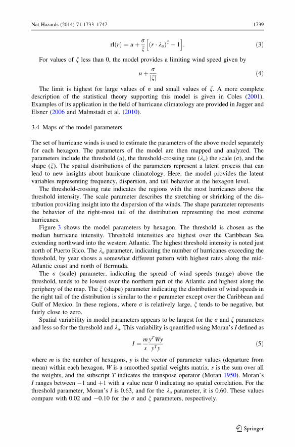
3.4 Maps of the model parameters

The set of hurricane winds is used to estimate the parameters of the above model separately

for each hexagon. The parameters of the model are then mapped and analyzed. The

parameters include the threshold (u), the threshold-crossing rate (ku) the scale (r), and the

shape (n). The spatial distributions of the parameters represent a latent process that can

lead to new insights about hurricane climatology. Here, the model provides the latent

variables representing frequency, dispersion, and tail behavior at the hexagon level.

The threshold-crossing rate indicates the regions with the most hurricanes above the

threshold intensity. The scale parameter describes the stretching or shrinking of the dis-

tribution providing insight into the dispersion of the winds. The shape parameter represents

the behavior of the right-most tail of the distribution representing the most extreme

hurricanes.

Figure 3 shows the model parameters by hexagon. The threshold is chosen as the

median hurricane intensity. Threshold intensities are highest over the Caribbean Sea

extending northward into the western Atlantic. The highest threshold intensity is noted just

north of Puerto Rico. The ku parameter, indicating the number of hurricanes exceeding the

threshold, by year shows a somewhat different pattern with highest rates along the mid-

Atlantic coast and north of Bermuda.

The r (scale) parameter, indicating the spread of wind speeds (range) above the

threshold, tends to be lowest over the northern part of the Atlantic and highest along the

periphery of the map. The n (shape) parameter indicating the distribution of wind speeds in

the right tail of the distribution is similar to the r parameter except over the Caribbean and

Gulf of Mexico. In these regions, where r is relatively large, n tends to be negative, but

fairly close to zero.

Spatial variability in model parameters appears to be largest for the r and n parameters

and less so for the threshold and ku. This variability is quantified using Moran’s I defined as

I ¼ m

s

yT Wy

yT yð5Þ

where m is the number of hexagons, y is the vector of parameter values (departure from

mean) within each hexagon, W is a smoothed spatial weights matrix, s is the sum over all

the weights, and the subscript T indicates the transpose operator (Moran 1950). Moran’s

I ranges between -1 and ?1 with a value near 0 indicating no spatial correlation. For the

threshold parameter, Moran’s I is 0.63, and for the ku parameter, it is 0.60. These values

compare with 0.02 and -0.10 for the r and n parameters, respectively.

Nat Hazards (2014) 71:1733–1747 1739

123

The positive spatial autocorrelation witnessed in these parameters is to be expected for

two reasons. First, the data are arbitrarily subset into hexagons for this project. An indi-

vidual hurricane passed through a series of hexagons and a maximum wind speed value per

hexagon was recorded. A maximum occurring in one hexagon from a given hurricane will

likely be very similar to another maximum occurring from the same hurricane at a nearby

hexagon. The second cause for the positive spatial autocorrelation is the physical

mechanics that control hurricane formation. Warm sea surface temperatures are necessary

for a hurricane to form. If a given hurricane event travelled over a warm area, and a

different hurricane event took a similar path over the same warmth at a different time, both

of these hurricanes could have similarly high maximum wind speed values.

The final output of the extreme value model is the return level for a specified return

period. Figure 4 shows the 30-year return level. Thirty years are chosen because this

represents the typical homeowners mortgage in the USA. The majority of the US coastline

within the study region, Gulf of Mexico, Caribbean Sea, and central Atlantic Ocean have a

30-year return level exceeding 50 ms-1, or a Category 3. This means that, on average,

a

Threshold (ms−1)

b

Rate (/year)

c

σ (ms−1)

d

ξ [Dimensionless]

36 38 40 42 44 46 48 50 0.00 0.05 0.10 0.15 0.20 0.25 0.30 0.35

0 5 10 15 20 25 30 35 −2.0 −1.5 −1.0 −0.5 0.0

Fig. 3 Latent model parameters mapped per hexagon. a Threshold (u) in ms-1, b rate (ku) of hurricanes peryear, c scale (r) in ms-1, and d shape (n)

1740 Nat Hazards (2014) 71:1733–1747

123

these areas can expect a 50 ms-1 wind speed to occur somewhere within the hexagon

every 30 years. This does not imply that a Category 3 hurricane will strike land within the

hexagons.

3.5 Limiting versus observed highest intensity

The limiting intensity depends on the ratio of r to n. Since both parameters show high

spatial variability, they are smoothed before applying Eq. 4. A hexagon has at most six

contiguous neighbors. The neighborhood average parameter value is the weighted sum

of the parameter values in the six neighbors, where each neighbor gets assigned a

weight of 1/6. Weights are adjusted accordingly for hexagons with fewer than six

neighbors.

The neighborhood average parameter value is then averaged with the parameter value in

the hexagon. For the r parameter, this is done using a simple average, but for the nparameter a weighted average is used with a weight of 0.75 on the neighborhood average.

Figure 5 shows the empirical maximum wind speed compared to the theoretical max-

imum wind speed and includes the difference between the two. The theoretical wind speed

can be understood as the highest possible wind speed that can be experienced within the

hexagon. Figure 5a suggests that the maximum possible wind speeds can occur over the

southeastern USA , the Gulf of Mexico, portions of northern Central America, and over the

northern tip of South America. Figure 5c shows the difference between the theoretical

highest intensity and the observed highest intensity. The largest differences occur over

Texas and portions of Central America. Here, the theoretical highest intensity is much

greater than the observed. This could be due to the influence of land in these hexagons.

Hurricanes passing over land often weaken, which could lead to the observed maximum

intensity being lower than the theoretical.

4 Sensitivity to SST

It is well known that the temperature of the oceans surface has a direct relationship with the

increasing intensity of hurricanes (DeMaria and Kaplan 1994). According to Emanuel

30 Year Return Level (ms−1)

30 35 40 45 50 55 60 65 70

Fig. 4 Thirty-year return levelin ms-1 mapped per hexagon

Nat Hazards (2014) 71:1733–1747 1741

123

(1988), a hurricane functions similarly to a Carnot engine, where the temperature of the

surface plays a role on the maximum potential intensity of a hurricane. The question of

which regions highest intensities are most sensitive to changes in SST is examined using

geographically weighted regression (GWR). A GWR model allows the relationship

between the response and the explanatory variable to vary across the domain (Brunsdon

et al. 1998; Fotheringham et al. 2000). GWR allows one to see where an explanatory

variable contributes strongly to the relationship and where it contributes weakly. It is

similar to a local linear regression. It is appropriate here because the latent variables and

the SST values can be modeled to provide insight into the way that hurricane character-

istics behave over space.

With GWR, the SST parameter is replaced by a vector of parameters (i.e., ku, r, n, or

the return level estimates), one for each hexagon. The relationship between the response

vector and the explanatory variables is expressed mathematically as

a

Theoretical Highest Intensity (ms−1)

b

Observed Highest Intensity (ms−1)

c

Theoretical − Observed Intensity (ms−1)

40 50 60 70 80 90 100 40 50 60 70 80 90 100

−5 0 5 10 15 20

Fig. 5 Comparison of the a theoretical maximum intensity in ms-1 per hexagon and the b observedmaximum intensity ms-1. A difference map is shown in (c)

1742 Nat Hazards (2014) 71:1733–1747

123

y ¼ XbðgÞ þ � ð6Þ

where g is a vector of geographic locations, here the set of hexagons with different latent

variables and

bðgÞ ¼ ðXT WXÞ�1XT Wy ð7Þ

where W is a weights matrix given by

W ¼ exp�D2

h2ð8Þ

where D is a matrix of pairwise distances between the hexagons and h is the bandwidth

(Fotheringham et al. 2000). The elements of the weights matrix, wij, are proportional to the

influence an individual hexagon j has on its neighboring hexagons i in determining the

relationship between X and y. Weights are determined by an inverse-distance function

(kernel) so that values in nearby hexagons have greater influence on the local relationship

compared with values in hexagons farther away. The bandwidth controls the amount of

smoothing. It is chosen as a trade-off between variance and bias. A bandwidth too narrow

(steep gradients on the kernel) results in large variations in the parameter estimates (large

variance). A bandwidth too wide leads to a large bias as the parameter estimates are

influenced by processes that do not represent the conditions locally. Here, an adaptive

kernel is chosen that allows the estimates to vary depending on the location of the samples.

The percent change in the intercept values of each variable across the hexagons pro-

vides information showing how sensitive the latent variables are to SST. There is a 22.1 %

change in the k, a 18.3 % change in the r, a -50.6 % change in the n, and a 4.1 % change

in the 30-year return level per degree SST. This suggests that the n parameter is the most

sensitive to SSTs. The n parameter represents the most extreme events (negative values

corresponding to more extreme events), so these results suggest that the maximum

intensity of hurricanes is most sensitive to a changing SST value compared to the other

model parameters.

a

SST Effect on Rate (hurricanes per year/oC)

b

Significance of Effect (t−value)

0.0026 0.0028 0.0030 0.0032 0.95 1.02 1.09 1.16 1.23

Fig. 6 a The effect of SST on the ku parameter with b statistical significance

Nat Hazards (2014) 71:1733–1747 1743

123

Local significance of the coefficients is found by dividing the SST coefficient by its

standard error. The ratio, called the t value, has a t-distribution under the null hypothesis of

a zero coefficient value. Regions of high t values (absolute value [2) denote areas of

statistical significance. The results for the GWR model of SST on k are shown in Fig. 6.

The marginal influence of SST on the number of hurricanes per year is shown along with

corresponding t values. In Fig. 6a, the rate of hurricane occurrence is affected more by

SSTs near the northern perimeter of the domain. This is because hurricanes do not occur

very often in these locations now because the required environmental conditions (i.e., the

SST values) are not met during most of the season. Any increase in the SST values may

alter the frequency of hurricanes in these hexagons. However, it can be seen in Fig. 6b that

no locations have a statistically significant relationship, as all t values are less than 2.

The results for the GWR model of SST on r are shown in Fig. 7. In Fig. 7a, it is shown

that the scale of hurricane wind speeds over the Caribbean Sea, Gulf of Mexico, and

western Atlantic is influenced by SST values more so than the other hexagons. This

suggests that as SSTs increase, the range of wind speeds occurring in these hexagons will

also increase. That is, more hurricanes of differing magnitudes will occur. The increased

SSTs could allow for the possibility of hurricanes to occur where the temperatures were

once too cold. The values are statistically significant.

The results for the GWR model of SST on n are shown in Fig. 8. In Fig. 8a, it is shown

that the parameter representing the most extreme values is most heavily influenced by SST

in the Gulf of Mexico, Caribbean Sea, and the very western portion of the Atlantic. Again,

lower values of n indicate more extreme events. These values are not statistically

significant.

Finally, the results for the GWR model of SST on the 30-year return level are shown in

Fig. 9. In Fig. 9a, SST values have the greatest influence over the western Atlantic, Gulf of

Mexico, and Caribbean Sea. As SSTs increase, the expected return level for a fixed time

period will increase. This result is consistent with the theory of maximum potential

intensity in hurricanes offered by Emanuel (1986). These values are statistically

significant.

Each of these plots suggests the overall influence of the ocean’s surface temperature on

individual hurricane characteristics. Although two parameters were not significant, it

a

SST Effect on σ (ms−1/ oC)

b

Significance of Effect (t−value)

0.40 0.42 0.44 0.46 0.48 0.50 2.1 2.2 2.3 2.4 2.5 2.6

Fig. 7 a The effect of SST on the scale parameter with b statistical significance

1744 Nat Hazards (2014) 71:1733–1747

123

provides an insight into hurricane characteristics that only a geographic approach can

supply.

5 Concluding remarks

Understanding local and regional hurricane risk is important for people living in harms

way, and decision makers responsible for evacuation and mitigation plans. Hurricane wind

speeds are mapped using a hexagonal tessellation over the Gulf of Mexico and North

Atlantic Ocean. This approach provides a unique insight into the way that hurricane

characteristics vary over space. A GPD extreme value model is used to calculate param-

eters of interest using the maximum hurricane wind speed values known to occur in each

hexagon. Specifically, the ku, or rate, the r, or scale, and the n, or shape, parameters are

cataloged. The rate represents the number of expected hurricanes per year and is highest

a

SST Effect on ξ ([Dimensionless]/ oC)

b

Significance of Effect (t−value)

0.009 0.010 0.011 0.012 0.013 0.014 0.015 0.6 0.67 0.74 0.81 0.88 0.95

Fig. 8 a The effect of SST on the shape parameter with b statistical significance

a

SST Effect on 30 Yr Wind (ms−1/oC)

b

Significance of Effect (t−value)

1.18 1.19 1.20 1.21 1.22 1.23 1.24 4.15 4.2 4.25 4.3 4.35 4.4

Fig. 9 a The effect of SST on the 30-year return level with b statistical significance

Nat Hazards (2014) 71:1733–1747 1745

123

over Florida, Bermuda, and the western Atlantic. These locations can expect the highest

number of hurricanes exceeding 33 ms-1 in any given year. The scale represents the

dispersion of wind speeds occurring in each hexagon and is highest over the Florida

peninsula, the Western Antilles Islands, and the southwestern Caribbean Sea. These

locations experience the widest range of wind speeds, meaning they receive many different

levels of hurricanes. The shape parameter represents the tail end of the distribution, where

stable model values nearest to -1 suggest the most extreme tails. The locations over the

Florida peninsula and Western Antilles Islands experience the most extreme events.

The 30-year return level is also visualized. Thirty years are chosen to represent the

average homeowner’s mortgage. The results estimated could provide potential and current

coastal homeowners with their overall risk during the time they might own a home. The

western Caribbean Sea and the Gulf of Mexico experience the highest wind return level for

30 years. The hexagons surrounding these locations also experience 30-year return levels

exceeding 50 ms-1, or a Category 3 hurricane.

The final portion of analysis was to test the relationship between the average August

through October SST values per hexagon with each of the parameters and the 30 year

return level using a GWR model. Based on the rate of change in the intercept value of the

GWR models, the n parameter is the most sensitive to a change in SST values. However,

both the n parameter and the ku parameter do not show statistically significant results. The

r parameter and the 30-year return level do have significant results. The model suggests

that as SSTs increase, the range of wind speeds occurring in the hexagons over the

Caribbean Sea, the Gulf of Mexico, and the western Atlantic will also increase. That is,

more hurricanes will occur of differing magnitudes. The model for the 30-year return level

suggests, again, that as SSTs increase, the expected return level for a fixed time period will

increase over those same locations. It is important to note that the parameters above are

dependent to some level on the size of the hexagon chosen.

These results provide additional questions for future research projects. One could

estimate how sensitive the parameters are to SST in cold versus warm El Nino Southern

Oscillation years, or estimate the influence of a warming trend on the latent model

parameters. Additional variables could be considered besides SST, including sunspot

numbers or stratospheric temperatures.

As the oceans’ surfaces increase in temperature, the maximum intensity for hurricanes

is expected to increase most significantly over the Gulf of Mexico, the Caribbean Sea, and

the western Atlantic. This is important for any population of people living in these loca-

tions because it provides them with a deeper understanding of the expected risk as they

move into the future.

Acknowledgments The author would like to thank James Elsner and Thomas Jagger for their guidance.

References

Atmospheric N, (NOAA) OA (2013) NOAA extended reconstructed sea surface temperature (SST) v3b.URL http://www.esrl.noaa.gov/psd/data/gridded/data.noaa.ersst.html

Brettschneider B (2008) Climatological hurricane landfall probability for the United States. J Appl MeteorolClimatol 47:704–716

Brunsdon C, Fotheringham A, Charlton M (1998) Geographically weighted regression: modelling spatialnon-stationarity. J Royal Stat Soc Ser D Stat 47:431–443

Chu P, Wang J (1998) Modeling return periods of tropical cyclone intensities in the vicinity of Hawaii.J Appl Meteorol Climatol 37:951–960

1746 Nat Hazards (2014) 71:1733–1747

123

Coles S (2001) An introduction to statistical modeling of extreme values. Springer, BerlinCooley D, Nychka D, Naveau P (2007) Bayesian spatial modeling of extreme precipitation return levels.

J Am Stat As 102:824–840DeMaria M, Kaplan J (1994) Sea surface temperature and the maximum intensity of Atlantic tropical

cyclones. J Clim 7:1324–1334Elsner J, Hodges R, Jagger T (2011) Spatial grids for hurricane climate research. Clim Dyn. doi:10.1007/

s00382-011-1066-5Elsner JB, Jagger, TH (2013) Hurricane climatology: a modern statistical guide using R. Oxford University

Press, New York, p 430Emanuel K (1986) An air–sea interaction theory for tropical cyclones. Part I: steady-state maintenance.

J Atmos Sci 43:585–604Emanuel K (1988) The maximum intensity of hurricanes. J Atmos Sci 45:1143–1155Emanuel K, Ravela S, Vivant E, Risi C (2006) A statistical deterministic approach to hurricane risk

assessment. Bull Am Meteorol Soc 87:299–314Esnard A, Sapat A, Mitsova D (2011) An index of relative displacement risk to hurricanes. Nat Hazards

59:833–859Fotheringham A, Brunsdon C, Charlton M (2000) Quantitative geography: perspectives on spatial data

analysis. Sage, LondonHeckert N, Simiu E, Whalen T (1998) Estimates of hurricane wind speeds by ‘peaks over threshold’ method.

J Struct Eng ASCE 124:445–449Jagger T, Elsner J (2006) Climatology models for extreme hurricane winds in the United States. J Clim

19:3220–3236Jagger T, Elsner J, Niu X (2001) A dynamic probability model of hurricane winds in coastal counties of the

United States. J Appl Meteorol 40:853–863Jarvinen BR, Neumann CJ, Davis MAS (1984) A tropical cyclone data tape for the North Atlantic basin,

1886–1983: Contents, limitations and uses. Tech. rep., NOAA Tech. Memo. NWS NHC 22, CoralGables, Florida

Joyner A, Rohli R (2010) Kernel density estimation of tropical cyclone frequencies in the North AtlanticBasin. Int J Geosci 1:121–129

Kantha L (2006) Time to replace the Saffir–Simpson Hurricane Scale?. EOS 87:3–6Keim B, Muller R, Stone G (2007) Spatiotemporal patterns and return periods of tropical storm and

hurricane strikes from Texas to Maine. J Clim 20:3498–3509Kotz S, Nadarajah S (2000) Extreme value distributions: theory and applications. Imperial College Press,

LondonLandsea C, Anderson C, Charles N, Clark G, Dunion J, Fernandez-Partagas J, Hungerford P, Neumann C,

Zimmer M (2004) The Atlantic hurricane database reanalysis project: documentation for the1851–1910 alterations and additions to the HURDAT database. In: Murnane R, Liu Kb (eds) Hurri-canes and typhoons: past, present, and future, Columbia University Press, Columbia, pp 177–221

Malmstadt J, Scheitlin K, Elsner J (2009) Florida hurricanes and damage costs. Southeast Geogr 49:108–131Malmstadt J, Elsner J, Jagger T (2010) Risk of strong hurricane winds to Florida cities. J Appl Meteorol

Climatol 49:2121–2132Moran P (1950) Notes on continuous stochastic phenomena. Biometrika 37:17–33NHC (2013) NHC data archive. URL http://www.nhc.noaa.gov/pastall.shtmlPalmen E (1948) On the formation and structure of the tropical hurricane. Geophysica 3:26–38Pielke R Jr, Gratz J, Landsea C, Collins D, Saunders M, Musulin R (2008) Normalized hurricane damage in

the United States: 1900–2005. Nat Hazards Rev 9:29–42R Development Core Team (2010) R: a language and environment for statistical computing. R Foundation

for Statistical Computing, Vienna. URL http://www.R-project.org ISBN 3-900051-07-0Simpson RH (1971) A proposed scale for ranking hurricanes by intensity. Minutes of the eighth noaa,

National Weather Service Hurricane Conference, Miami, FloridaSimpson R, Lawrence M (1971) Atlantic hurricane frequencies along the US coastline. Technical Memo to

the National Weather Service SR-58, National Oceanic and Atmospheric AdministrationUSGS (2005) Hurricane hazards: a national threat. URL http://pubs.usgs.gov/fs/2005/3121/2005-3121.pdf

Nat Hazards (2014) 71:1733–1747 1747

123